Biomass Energy and Competition for Land*

by

John Reilly

Sergey Paltsev

Joint Program on the Science and Policy of Global Change, Massachusetts Institute of Technology, Cambridge, USA

GTAP Working Paper No. 46 2008

*Chapter 8 of the forthcoming book Economic Analysis of Land Use in Global Climate Change Policy, edited by Thomas W. Hertel, Steven Rose, and Richard S.J. Tol

2

BIOMASS ENERGY AND COMPETITION FOR LAND

John Reilly and Sergey Paltsev

Abstract

We describe an approach for incorporating biomass energy production and competition for land into the MIT Emissions Prediction and Policy Analysis (EPPA) model, a computable general equilibrium model of the world economy. We examine multiple scenarios where greenhouse gas emissions are abated or not. The global increase in biomass energy use in a reference scenario (without climate change policy) is about 30 EJ/year by 2050 and about 180 EJ/year by 2100. This deployment is driven primarily by a world oil price that in the year 2100 is over 4.5 times the price in the year 2000. In the scenarios of stabilization of greenhouse gas concentrations, the global biomass energy production increases to 50-150 EJ/year by 2050 and 220-250 EJ/year by 2100. The estimated area of land required to produce 180-250 EJ/year is about 1 Gha, which is an equivalent of the current global cultivated area. In the USA we find that under a stringent climate policy biofuels could supply about 55% of USA liquid fuel demand, but if the biofuels were produced domestically the USA would turn from a substantial net exporter of agricultural goods ($20 billion) to a large net importer ($80 billion). The general conclusion is that the scale of energy use in the USA and the world relative to biomass potential is so large that a biofuel industry that was supplying a substantial share of liquid fuel demand would have very significant effects on land use and conventional agricultural markets.

3

Table of Contents 1. Introduction ..................................................................................................................4 2. Biomass Energy Technologies .....................................................................................5 3. The EPPA Model: Biomass Technologies and Land-Use ............................................8 3.1 Overview of the EPPA Model ......................................................................................8 3.2 Specification of Biomass Technologies .......................................................................9 3.3 Relationship to Physical Land Use .............................................................................12 4. Illustrative Scenarios ..................................................................................................13 4.1 Atmospheric Stabilization of Greenhouse Gases .......................................................14 4.2 The Potential Role of Bioenergy in US GHG Policy .................................................16 5. Conclusion ..................................................................................................................20 6. References ..................................................................................................................23

Table 1. World Land Area and a Potential for Energy from Biomass ...................27 Table 2. U.S. Land Area and a Potential for Energy from Biomass ......................28

Table 3. Regions and Sectors in the EPPA4 Model ...............................................29 Table 4. Mark-ups and Input Shares for Bio-oil and Bio-electric Technologies ...30 Table 5. Reference Values for Elasticities in Bio-oil and Bio-electric Technologies ............................................................................................31 Table 6. US Land Area (Mha) Required for Biomass Production in CCSP Scenarios ..................................................................................................32 Table 7. Global Land Area (Mha) Required for Biomass Production in CCSP

Scenarios ..................................................................................................32 Table 8. US Land Area (Mha) Required for Biomass Production in US Congressional Analysis Scenarios ............................................................32 Table 9. Global Land Area (Mha) Required for Biomass Production in US Congressional Analysis Scenarios ............................................................32

Figure 1. Structure of Biotechnology Production Functions ...................................33 Figure 2. Global Biomass Production Across Scenarios .........................................34 Figure 3. U.S. Biomass Production Across Scenarios .............................................35 Figure 4. Global Primary Energy Consumption in the Reference ...........................36 Figure 5. Global Primary Energy in the Level 3 Scenario .......................................37 Figure 6. Global Primary Energy in the Level 1 Scenario .......................................38 Figure 7. Land Price and Agriculture Output Price in USA in the Level 2 Scenario Compared with the Reference Prices ........................................39 Figure 8. Liquid Biofuel Use, With and Without International Trade in Biofuels ..40

Figure 9. Net Agricultural Exports in the 167 Bmt Case, With and Without Biofuels Trading .........................................................................41 Figure 10. Indexes of Agriculture Output Price, Land Price, and Agriculture Production in USA ................................................................42

4

BIOMASS ENERGY AND COMPETITION FOR LAND

John Reilly and Sergey Paltsev

1. INTRODUCTION

Biomass energy can be used to avoid greenhouse gas emissions from fossil fuels by

providing equivalent energy services: electricity, transportation fuels and heat if a

significant amount of fossil fuel is not used in its production (IPCC, 2000). In 2001,

global biomass energy use for cooking and heating was 39 exajoules (EJ), or 9.3% of the

global primary energy use, and biomass energy use for electricity and fuel generation was

6 EJ, or 1.4% of global primary energy use (IEA, 2001; Smeets and Faaij, 2007). The

estimates of the global bioenergy production potential vary substantially from a low

estimate of 350 EJ/year (Fisher and Schrattenholzer, 2001) to as much as 1300 EJ/year

(IEA, 2001) to 2900 EJ/year (Obersteiner et al., 2002; Hall and Rosillio-Calle, 1998).

Because global demand for food is also expected to double over the next 50 years

(Fedoroff and Cohen, 1999), increased biofuel production competes with agricultural

land needed for food production.

In this paper we present a methodology for incorporating biomass production

technologies into a Computable General Equilibrium (CGE) model. A key strength of

CGE models is their ability to model economy-wide effects of policies and other external

shocks, rather than just individual markets or sectors. We integrate biomass production

technologies and competition for land into the MIT Emissions Prediction and Policy

Analysis (EPPA) model (Paltsev et al., 2005) which has been widely used to study

climate change policy. We apply the model to estimate biomass production in different

scenarios of greenhouse gas emissions abatement developed by the U.S. Climate Change

Science Program (CCSP, 2006). We also consider several scenarios that span the range of

current U.S. Congress proposals to control U.S. greenhouse gas emissions (Paltsev et al.,

2007). In these estimates, competition for labor, capital, land, and other resources in the

economy is explicitly represented in the model.

5

The paper is organized in the following way. In the next section we describe biomass

energy production. Section 3 presents the changes in the EPPA model structure, which

we have made to incorporate bioenergy production technologies and competition for

land. In Section 4 we examine several scenarios where greenhouse gas emissions are

controlled or not, and show the impacts on biomass production, land prices, and the

agricultural sector in the U.S. Section 5 concludes.

2. BIOMASS ENERGY TECHNOLOGIES

There are several ways biomass is or can be used for energy production. Currently, most

biomass is used in the form of woodfuel and manure for cooking and heating. Out of 39

EJ of traditional biomass use in 2002, 21 EJ is consumed in the form of woodfuel, and

the rest is from manure, waste and agriculture residues (Smeets and Faaij, 2007). In our

paper we do not discuss the traditional use of biomass and focus on so called “modern”

and “advanced” biomass energy technologies for transportation fuel and electricity.

Liquid and gaseous transport fuels derived from a range of biomass sources are

technically feasible. They include methanol, ethanol, di-methyl esters, pyrolytic oil,

Fischer-Tropsch gasoline and distillate, and biodiesel from vegetable oil crops (IPCC,

2001). Currently, the largest sources of commercially produced ethanol are from sugar

cane in Brazil and from corn in the USA. Biodiesel is produced from rapeseed in Europe.

In most cases, current biofuel production is subject to government support and subsidies.

In the USA, ethanol is used mostly as an oxygenating fuel additive to reduce carbon

monoxide emissions to meet environmental standards. Thus, it is not competing directly

with gasoline on the basis of its energy content. As for other uses of biomass, crop and

wood residues, animal manures and industrial organic wastes are currently used to

generate biogas. Animal fats can also be converted into biodiesel.

Energy yield from different biomass sources can vary substantially. Vegetable oil crops

have a relatively low energy yields (40-80 gigajoules(GJ)/hectare(ha)/year) compared

6

with crops grown for cellulose or starch/sugar (200-300 GJ/ha/year). According to IPCC

(2001), high yielding short rotation forest crops or C4 plants (e.g., sugar cane or

sorghum) can give stored energy equivalent of over 400 GJ/ha/year.

Woody crops are another alternative. The IPCC (2001) reports a commercial plot in

Sweden with a yield of 4.2 oven-dry tonnes(odt)/ha/year, and anticipates that with better

technologies, management and experience the yield from woody crops can be up to 10

odt/ha/year. Using the number for a higher heating value1 (20 GJ/odt) that Smeets and

Faaj (2007) used in their study of bioenergy potential from forestry, we can estimate a

potential of 84-200 GJ/ha/year yield for woody biomass.

Hybrid poplar, willow, and bamboo are some of the quick-growing trees and grasses that

may serve as the fuel source for a biomass power plant, because of the high amount of

lignins, a glue-like binder, present in their structures, which are largely composed of

cellulose. Such so-called "lignocellulose" biomass sources can potentially be converted

into ethanol via fermentation or into a liquid fuel via a high-temperature process.

Land that is needed to grow energy crops competes with land used for food and wood

production unless surplus land is available. For example, Smeets and Faaij (2007)

estimate a global theoretical potential of biomass from forestry in 2050 as 112 EJ/year.

They reduce this number to 71 EJ/year after considering demand for wood production for

other than bioenergy use. The number is decreased further to 15 EJ/year when economic

considerations are included into their analysis. In the study of biodiesel use in Europe,

Frondel and Peters (2007) found that to meet the EU target for biofuels 11.2 Mha are

required in 2010, which is 13.6% of total arable land in the EU25. An IEA (2003) study

estimates that replacing 10% of fossil fuels by bioenergy in 2020 would require 38% of

total acreage in the EU15. These analyses, while providing useful benchmarks, typically

take market conditions as given, whereas prices and markets will change in the future and

1 Higher heating value, or HHV, of a fuel is defined as the amount of heat released by a specified quantity (initially at 25°C) once it is combusted and the products have returned to a temperature of 25°C.

7

will depend on, for example, the existence of greenhouse gas mitigation policies that

could create additional incentives for biofuels production.

Table 1 provides a rough estimate of a global potential for energy from biomass based on

the total land area. IPCC (2001) used an average energy yield of 300 GJ/ha/year for its

projection of a technical energy potential from biomass by 2050. The area not suitable for

cultivation is about half of the total Earth land area of 15.12 Gha and it includes tropical

savannas, deserts and semideserts, tundra, and wetlands. Using the numbers for

converting area in hectares into energy yield, we estimate the global potential of around

2100 EJ/year from biomass. One can increase or decrease this estimate by including or

excluding different land types from the calculation. Assuming a conversion efficiency of

40 percent from biomass to the final liquid energy product, we estimate a potential of 840

EJ/year of liquid energy product from biomass. Table 2 presents a similar calculation for

the U.S., where a potential for a dry bioenergy is about 200 EJ/year and for a potential for

a liquid fuel from biomass is about 80 EJ/year. Note that these are maximum potential

estimates that assume that all land that currently is used for food, livestock, and wood

production would be used for biomass production.

A recent study by the U.S. Government (CCSP, 2006) projects an increase in the global

energy use from about 400 EJ/year in 2000 to 700-1000 EJ/year in 2050, and to 1275-

1500 EJ/year in 2100. The corresponding numbers for the U.S. are about 100 EJ/year in

2000, 120-170 EJ/year in 2050, and 110-220 EJ/year in 2100. These numbers suggest that

energy from biomass alone would not be able to satisfy global needs even if all land is

converted to biomass production, unless a major breakthrough in technology occurs.

Concerns about national energy security and mitigation of CO2 have generated much

interest in biofuels, although a recent cost-benefit study (Hill et al., 2006) has found that

even if all of the U.S. production of corn and soybean is dedicated to biofuels, this supply

would meet only 12% and 6% of the U. S. demand for gasoline and diesel, respectively.

Other work has shown that the climate benefit of this fuel, using current production

techniques is limited because of the fossil fuel used in the production of the crop and

8

processing of biomass (Brinkman et al., 2006). Advanced synfuel hydrocarbons or

cellulosic ethanol produced from biomass could provide much greater supplies of fuel

and environmental benefits than current technologies. Current studies thus raise a number

of issues and guide the direction of our representation of biofuels in a CGE model to

estimate economy-wide effects of different policies, which we discuss in more detail in

the next Section.

3. THE EPPA MODEL: BIOMASS TECHNOLOGIES AND LAND-USE

3.1 Overview of the EPPA Model

The MIT Emissions Prediction and Policy Analysis (EPPA) model is a recursive-

dynamic multi-regional computable general equilibrium (CGE) model of the world

economy (Paltsev et al., 2005). EPPA is built on the GTAP data set, which

accommodates a consistent representation of energy markets in physical units as well as

detailed accounts of regional production and bilateral trade flows (Hertel, 1997;

Dimaranan and McDougall, 2002). Besides the GTAP data set, EPPA uses additional

data for greenhouse gas (CO2, CH4, N2O, HFCs, PFCs, and SF6) and air pollutant

emissions (SO2, NOx, black carbon, organic carbon, NH3, CO, VOC) based on United

States EPA inventory data and projects, including endogenous costing of the abatement

of non-CO2 GHGs. For use in EPPA the GTAP dataset is aggregated into the 16 regions

and 21 sectors shown in Table 3. The base year of the EPPA model is 1997. From 2000

onward it is solved recursively at 5-year intervals. The EPPA model production and

consumption sectors are represented by nested Constant Elasticity of Substitution (CES)

production functions (or the Cobb-Douglas and Leontief special cases of the CES). The

model is written in GAMS-MPSGE (Rutherford, 1995). It has been used in a wide variety

of policy applications (e.g., Jacoby et al., 1997; Reilly et al., 1999; Paltsev et al., 2003;

Babiker, Reilly and Metcalf, 2003; Reilly and Paltsev, 2006; CCSP, 2006).

Because of the focus on climate policy, the model further disaggregates the GTAP data

for energy supply technologies and includes a number of energy supply technologies that

9

were not in widespread use in 1997 but could take market share in the future under

changed energy price or climate policy conditions. Bottom-up engineering details are

incorporated in EPPA in the representation of these alternative energy supply

technologies.

3.2 Specification of Biomass Technologies

We introduce two technologies which use biomass: electricity production from biomass

and a liquid fuel production from biomass. Both use land and a combination of capital,

labor and other inputs. They compete for land with agricultural sectors of the economy.

These technologies endogenously enter the market place if and when they become

economically competitive with existing technologies. Competitiveness of different

technologies depends on the endogenously determined prices for all inputs, as those

prices depend on depletion of resources, climate policy, and other forces driving

economic growth such as the savings, investment, energy-efficiency improvements, and

the productivity of labor.

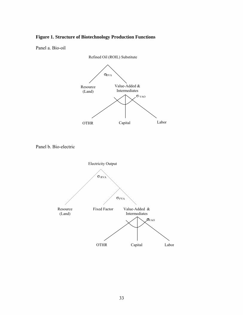
The production structures for biomass technologies are shown in Figure 1. Production of

liquid fuel from biomass (panel a) uses capital, labor, and intermediate inputs from the

Other Industries (OTHR) sector. Production of electricity from biomass (panel b) has a

very similar production structure, except that it includes an additional fixed factor to slow

initial penetration as described in more detail in McFarland et al. (2004). Land is

modeled as a non-depletable resource whose productivity is augmented exogenously. The

rate of land productivity augmentation in EPPA regions is as follows: USA, Central and

South America (LAM), Africa (AFR), Rest of World (ROW) regions, 1.5% per year; for

India (IND) and Indonesia (IDZ), land productivity growth is decreasing from 3% to 2%

between 1997 to 2050, stays at 2% from 2050-2075, and at 1.5% from 2075-2100;

Mexico (MEX) and China (CHN), 2% per year; all other regions, 1% per year. As

reviewed in Reilly and Fuglie (1998), historically crop yields have grown from 1% to 3%

per year, although many believe that growth may be slowing, and so maintaining such

rates for 100 years would seem difficult. On the other hand, agronomists identify a factor

four difference between commercial yields and potential yields for key crops such as rice.

10

In addition, the rate of augmentation in EPPA applies to a highly aggregated agricultural

sector that includes crops, livestock, and forestry. The land input, especially for forestry

and livestock, includes much land where the economic yield is very low because some of

the land suffers from shortcomings that make it currently not very productive as cropland.

In addition, productivity in many parts of the world is low because modern technology is

poorly diffused. Innovation that removed constraints and diffusion of best practices could

significantly increase the productivity of “average” land even if conventionally measured

yields of crops on existing cropland did not increase.

Note that the production of the biomass and the conversion of the biomass to fuel or

electricity are collapsed into a single nest (i.e., the capital and labor needed for both

growing and converting the biomass to a final fuel are combined). These are

parameterized to represent a conversion efficiency of 40 percent from biomass to the

final energy product. This conversion efficiency also assumes that process energy needed

for bio-fuel production is from biomass. While obviously simplified, a more detailed

nest and input structure would entail describing in greater detail a technology that is not

fully developed and is likely to change considerably as technology advances.

Table 4 presents mark-ups and input shares for Bio-Oil and Bio-Electricity technologies.

By convention, we set input shares in each technology so that they sum to 1.0. We then

separately identify a multiplicative mark-up factor that describes the cost of the advanced

technology relative to the existing technology against which it competes in the base year2.

This mark-up is a multiplier for all inputs. For example, the mark-up of the Bio-Oil

technology in the USA region is 2.1, implying that this technology would be

economically competitive at a refined oil price that is 2.1 times that in the reference year

(1997) if there were no changes in the price of inputs used either in refined oil production

or in production of liquid fuel from biomass. As with conventional technologies, the

ability to substitute between inputs in response to changes in relative prices is controlled

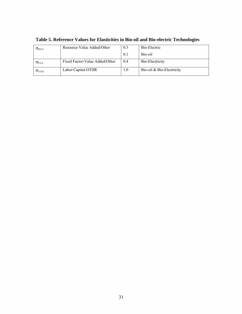
by the elasticities of substitution, which are given in Table 5.

2 For more discussion on modeling advanced technologies in EPPA, see McFarland et al (2004), Paltsev et al (2005), Jacoby et al (2006).

11

As identified in the previous section, corn and soybean based biofuel liquid production

potential is relatively limited, and current biomass production processes in the USA (e.g.,

ethanol from corn) often use fossil energy thus releasing nearly as much CO2 as is offset

when the ethanol is used to replace gasoline. Potential production from these sources is

too limited to ever play a role much beyond that of producing enough ethanol to serve as

an oxygenating additive to gasoline in the USA. Our modeling focus is thus to represent

advanced technologies that can make use of a broader biomass feedstock, thereby

achieving levels of production that can make a more substantial contribution to energy

needs. For our purposes, there is also little reason to represent CO2-intensive production

processes because in scenarios where carbon is priced their cost would escalate with the

carbon price just as would the price of conventional petroleum products, and thus it

would never be competitive. An alternative strategy is to introduce several competing

biomass energy technologies with different cost specifications and technology

specifications. As a first step, our approach is to specify a technology that is likely to

dominate others over the longer term. These considerations drive our parameterization of

the bioenergy technologies.

We considered early estimates of global resource potential and economics (Edmonds and

Reilly, 1985) and recent reviews of potential (Moreira, 2004; Berndes et al., 2003) and

the economics of liquid fuels (Hamelinck et al., 2005) and bio-electricity (International

Energy Agency, 1997). Regarding cost, Hamelinck et al. (2005), estimate costs of

lignocellusic conversion of ethanol of 9 to 13 €/GJ compared with 8 to 12 and eventually

5 to 7 €/GJ for methanol production from biomass. They compare these to before tax

costs of gasoline production of 4 to 6 €/GJ. Our estimated mark-up of 2.1 is thus

consistent with the lower end of the near and mid term costs for ethanol or methanol. We

parameterize land requirements per unit of biofuel produced to be consistent with the 300

GJ/ha/year.

12

3.3 Relationship to Physical Land Use

The CGE framework measures all inputs in monetary units. If we wish to inform our

parameterization of input shares, land productivity, and conversion efficiencies from

agro-engineering studies, we must translate them into units used in the CGE model. Thus,

to convert the 300 GJ/ha/year we need an estimate of the land price. We assume the

productivity rate is for “average” cropland, and thus use the average USA cropland price

and our assumption of 40% efficiency of conversion to estimate the initial value share of

land in biofuel production. The amount of biofuel liquid produced in GJ must then

compete with petroleum products in the base year with input shares adding to 1.0, for

which we have the GTAP supplemental physical energy accounts. This ensures that the

physical energy produced by the Bio-Oil technology is equal to the petroleum product for

which it is a perfectly competitive good. The mark-up multipliers on other inputs in the

production technology then produce a final cost of the biofuel technology reflecting

existing cost studies of biofuels relative to gasoline. The same approach is used for Bio-

Electricity where the comparison of energy output is with the conventional electricity

sector for which Bio-Electricity produces a perfectly competitive substitute.

The same calculations that allow us to parameterize the production technology then allow

us to back out estimates of physical land used in bioenergy production. An important

caveat to this result is that land is a homogeneous input in the version of the EPPA model

used here, and thus the quantity of land in hectares should be considered as an “average

cropland equivalent.” Obviously, land quality and land prices vary, and we are modeling

productivity of land to change over time. The National Income and Product Accounting

approach, that is the basis of CGE data, takes the value of different land as an indication

of it marginal product. The implication for our CGE model is that when we use a unit of

land in monetary terms we are using a comparable productivity unit—an “average

cropland equivalent”. In reality, this could be more hectares of less productive (less

valuable) land or fewer hectares of more productive (more valuable land). By

parameterizing bioenergy in this way it implies that productivity of land in terms of

GJ/ha/year is directly proportional to the land price as it varies across different land types

in the base year. While this is not strictly true, as a first approximation it is reasonable.

13

Also note that a homogenous land input implies that land is perfectly mobile among

sectors, albeit there are only three land using sectors in the version of the EPPA model

used here: (1) an aggregate agriculture sector that includes all crops, livestock, and

forestry production; (2) biofuels liquids; and (3) electricity from biofuels. At this level of

aggregation land conversion is not well-defined because we are not resolving whether the

biofuel land is coming from forest, cropland, pasture, or unmanaged land.

To approximate the physical amount of land used in bioenergy we use the following

procedure. As described in the notes to Tables 1 and 2, current estimates are that land

could reasonably achieve an average production of 15 odt/ha/year of biomass. This is

above what is often achieved under current practices, but is not as high as expected to be

achieved with genetically modified plants and other productivity enhancing

developments. The IPCC (2001) uses the 15 odt/ha/yr to estimate biomass production in

2050. We similarly assume that this production rate applies to 2050. However, as

discussed in the previous section, land in EPPA is subject to exogenous augmentation

that varies by region. We thus apply the rates of productivity change assumed in EPPA

from 1997 to 2100, and index the productivity change so that physical production is 15

odt/ha/year in 2050. We apply the 40% conversion efficiency in the production of

biofuels (i.e., 60% loss related to energy used in the process of producing the marketable

fuel) to estimate the total biomass (and land requirement). This allows us to make

approximate side calculations of the amount land required in simulations as reported

below.

4. ILLUSTRATIVE SCENARIOS

The EPPA model has been used in a variety of recent policy applications. We draw on

two of those to illustrate the modeling of bioenergy in EPPA, and the potential role of

biomass as an energy supplier. The first of these applications involves scenarios of

atmospheric stabilization of greenhouse gases. The second study involves investigation of

USA GHG mitigation policies that have been proposed in recent Congressional

14

legislation. These applications allow us to focus both on the global bioenergy potential

and on some specific issues with regard to USA bioenergy.

4.1 Atmospheric Stabilization of Greenhouse Gases

To illustrate how the EPPA model performs in terms of bioenergy technologies, we use

the reference and four stabilization scenarios employed in the recent U.S. Climate

Change Science Program (CCSP, 2006). The four stabilization scenarios were developed

so that the increased radiative forcing from greenhouse gases was constrained to no more

than 3.4 W/m2 for Level 1, 4.7 W/m2 for Level 2, 5.8 W/m2 for Level 3, and 6.7 W/m2 for

Level 4. These levels were defined as increases above the preindustrial level, so they

include the roughly 2.2 W/m2 increase that has already occurred as of the year 2000.

These radiative forcing levels were chosen so that the associated CO2 concentrations

would be roughly 450 ppm, 550 ppm, 650 ppm, and 750 ppm.

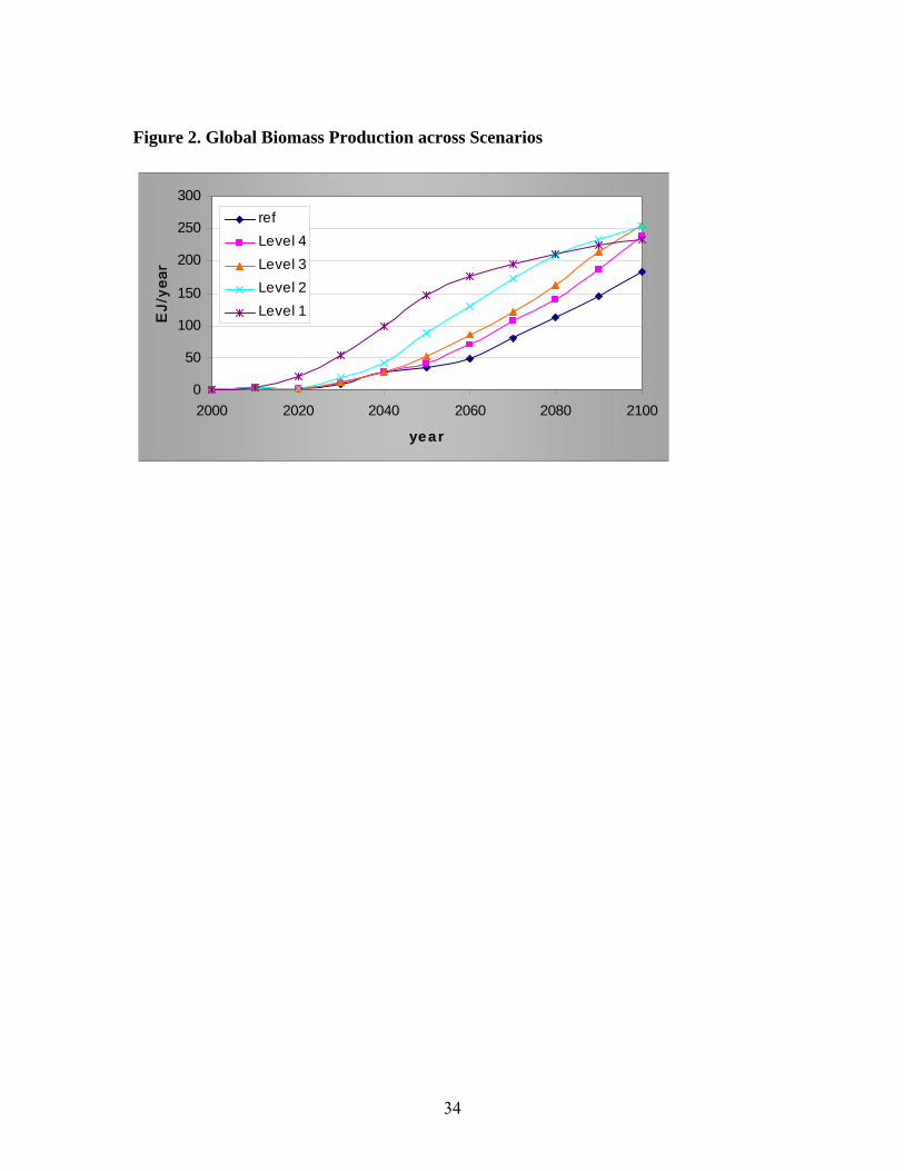
In these scenarios we do not consider climate feedbacks. The numbers for biomass

represent only the production of biomass energy from the advanced technologies we have

represented in EPPA and do not include, for example, the own-use of wood wastes for

energy in the forest products industry. Those are implicit in the underlying data in the

sense that to the extent the forest product industry uses its own waste for energy, it

purchases less commercial energy. Similarly, to the extent that traditional biomass energy

is a substantial source of energy in developing countries it implies less purchase of

commercial energy.3 Figures 2 and 3 present “advanced” biomass production for the

world (Figure2) and in the U.S. (Figure 3) across the scenarios. The reference scenario

exhibits a strongly growing production of bio-fuels beginning after the year 2020.

Deployment is driven primarily by a world oil price that in the year 2100 is over 4.5

times the price in the year 2000. In the stabilization scenarios, global biomass production

3 Developing countries are likely to transition away from this non-commercial biomass use as they become richer, and this is likely one reason why we do not observe rates of energy intensity of GDP improvements in developing countries that we observe in developed countries. EPPA accommodates this transition by including lower rates of Autonomous Energy Efficiency Improvement in poorer countries, thus capturing the tendency this would have to increase commercial fuel use without explicitly accounting for non-traditional biomass use.

15

reaches 250 EJ/year, and the U.S. biomass production is in the 40-48 EJ/year range by

2100.

The types of land are not modeled explicitly in the current version of the model, but as

described in Section 3.3 we can make some side calculations of the amount of “average”

physical land that would be required. Such estimates for the US are provided in Table 6

and for the global total in Table 7. As evident from these tables, the land area requirement

is substantial even with the assumed significant improvement in productivity of land. In

the US, estimated land in bioenergy reaches in 2100 about 150 to 190 million hectares

across the scenarios, including the reference. Globally land area required for bioenergy

production is just over 700 million hectares in the reference case and is about 1 billion

hectares in the stabilization scenarios in 2100. For the US this level of land use is about

the same as the 177 million hectares of current cropland (as shown in Table 2), and

similarly for the world the 1 billion hectares is on the order of total current cultivated land

which is reported in IPCC (2001) at 897 million hectares4. Improved land productivity

leads to some reduction in land required for biofuels after 2050.

Figures 4-6 show the composition of global primary energy for the reference, Level 3,

and Level 1 scenarios5. Across the stabilization scenarios, the energy system relies more

heavily on non-fossil energy sources, and biomass energy plays a major role. Total

energy consumption, while still higher than current levels, is lower in stabilization

scenarios than in the reference scenarios, and carbon capture and storage (CCS)

technologies are widely deployed. While we do not report here electricity production by

technology and so do not see the contribution of Bio-Electricity, we find that the Bio-

Electricity technology is rarely if ever used. Coal continues to be an inexpensive source

of energy for power generation in the reference case and so Bio-Electricity does not

compete. In the stabilization scenarios, there are a variety of low carbon and carbon-free

generation technologies that outcompete Bio-Electricity. An important reason for this is

that the demand for Bio-Oil is so strong because there are no other good low-carbon

4 IPCC (2000) reports 1.6 Gha for global croplands. IPCC (2001) reports 0.897 Gha for global cultivated land in 1990 and 2.495 Gha for total land with crop production potential. 5 See CCSP (2006) for the corresponding numbers for the other scenarios.

16

substitutes for petroleum products used in the transportation sector. As a result, this

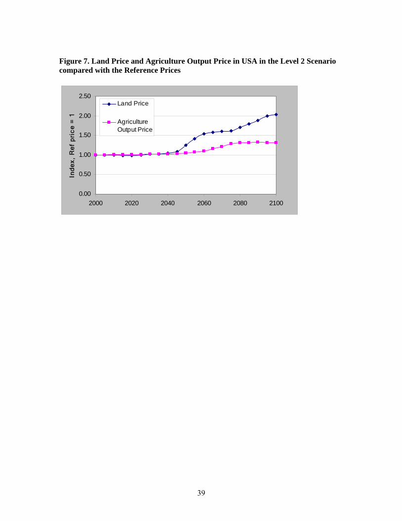
demand drives up the land price and raises the cost of Bio-Electricity. Figure 7 presents

land price and agriculture output price impacts in USA in the Level 2 scenario compared

with reference prices for land and the output of agriculture sector. Land prices in USA

more than double due to increased biomass demand. At the same time, an increase in an

agriculture output price index (which does not include biomass produced for bioliquids

and bioelectricity) is only about 30% by the end of century. There is a corresponding

reduction in output of non-biomass agriculture sector by 12% by the end of century,

which reflects a greater competition for land from biomass production.

4.2 The potential role of bioenergy in US GHG policy

In 2003 Senators McCain and Lieberman introduced cap and trade legislation in the U.S.

Senate. For a discussion and analysis see Paltsev et al. (2003). Interest in GHG mitigation

legislation in the U.S. Congress has grown substantially since then, and as of 2007 there

are several proposals for cap and trade systems in the US including a revised proposal by

McCain and Lieberman. Compared with the earlier proposals, these Bills envision much

steeper cuts in USA emissions and extend cap-&-trade system through 2050. Some of

these envisioned emissions in the USA as much as 80% below the 1990 level by 2050.

This would be as much as a 91% reduction from the EPPA reference emissions projected

in 2050. Such a steep reduction cannot avoid making significant cuts from CO2 emissions

from transportation which currently accounts for about 33% of USA CO2 emissions

related to fossil fuel combustion (EIA, 2006a). While improved efficiency of the vehicle

fleet might contribute to reductions, it is hard to imagine sufficient improvements in that

regard. Of the contending alternative fuels—hydrogen, electric vehicles, biofuels—the

biofuel option appears closest to being technologically ready for commercialization. A

more complete discussion and analysis of current Congressional proposals is provided in

Paltsev et al. (2007). Here we focus on the role of bioenergy under these mitigation

scenarios.

17

To capture the basic features of different proposals, we assume that the policy enters into

force in 2012. The initial allowance level is set to the (estimated6) USA GHG emissions

in 2008 and the annual allowance allocation follows a linear path through 2050 to (1)

2008 emissions levels; (2) 50% below 1990; and (3) 80% below 1990. Over the 2012 to

2050 period the cumulative allowance allocations under these three scenarios are 287,

203, and 167 billion metric tons (bmt), or gigatons, of carbon dioxide equivalent (CO2-e)

emissions. EPPA simulates every 5 years and so the initial year for which the policy is in

place in the simulations is 2015. We designate these scenarios with the shorthand labels

287 bmt, 203 bmt, and 167 bmt. We approximate banking of allowances in the USA, as

allowed in several of the proposals, by meeting the target with a CO2-e price path that

rises at the rate of interest, assumed to be 4%. We assume that other developed countries

pursue a policy whereby their emissions also fall to 50% below 1990 levels by 2050, and

a policy whereby all other regions return to (our projected) 2015 level of emissions in

2025, holding at that level until 2035 when the emissions cap drops to their year 2000

level of GHG emissions. We do not allow international emissions trading but we do

simulate economy-wide trading among greenhouse gases at their Global Warming

Potential (GWP) value. All prices are thus CO2-equivalent prices (CO2-e). The carbon

dioxide prices required to meet these policy targets in the initial projection year (2015)

are $18, $41, and $53/t CO2-e for the 287, 203, and 167 bmt cases, respectively.

In one set of scenarios we allow unrestricted trade in biofuels. We find significant

amounts of biofuel use in the USA in the more stringent scenarios but that nearly all of it

is imported. There are currently tariffs on biofuel import into the USA, and one of the

reasons biomass is of interest in the USA because it could be produced from domestic

resources. We thus consider a separate set of scenarios where all biofuel use in the USA

(and in other regions of the world) must be produced domestically. We designate these

with the extension NobioTR.

6 We estimate 2008 emissions by extrapolating from the most recent USA inventory for 2005 at the 1% per year growth in GHG emissions observed over the past decade.

18

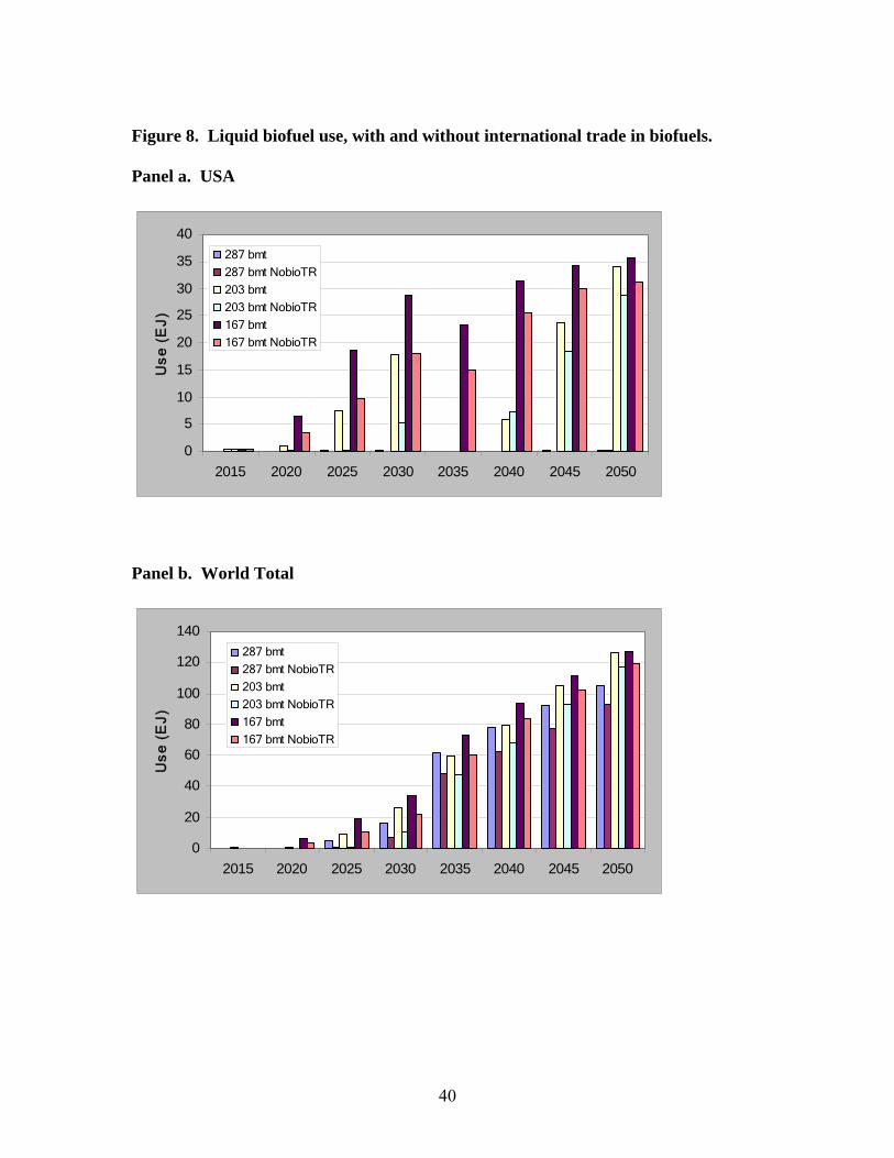
Turning to the specific simulation results, we find that USA biofuel use is substantial in

the 203 bmt and 167 bmt cases, rising to 30 to 35 EJ and in the core cases (Figure 8,

panel a). The 287 bmt case results in very little USA biofuels consumption—less than 1

EJ in any year, and so we do not show it in the Figure 8. World liquid biofuel use is

substantial in all three cases, reaching 100 to 120 EJ, because the ROW is pursuing the

same strong GHG policy even as we vary the policy in the USA. Thus, the main

difference in the world total is the changes in biofuels use in the USA. If the USA

pursued the 287 bmt case and the rest of the world did nothing, there would be substantial

biofuels use in the USA. However, when the rest of the world pursues a GHG mitigation

policy, the USA cannot compete in the biofuels market. When we restrict biofuel use

only to domestically produced, we find somewhat lower biofuels use in the USA and in

the total for the world (Figure 8, panel b). However, biofuel use, and hence production, in

the USA is substantial, falling in the 25 to 30 EJ range by the end of the period rather

than the 30 to 35 EJ. Biofuel has substantially displaced petroleum products accounting

for nearly 55% of all liquid fuels in the USA

Again, based on the approach described in Section 3.3 we can make side calculations on

the amount of land required for biofuels production in these scenarios. Such estimates are

reported in Tables 8 for the US and in Table 9 for the global total. The interesting thing to

note is that in the policy cases the land required by 2050 approaches or exceeds that in

the CCSP scenarios in 2100. The reason is that these policy scenarios require a much

more rapid reduction in greenhouse gas emissions, particularly in developed countries

with large transportation fuel demand. Thus, the demand for carbon-free fuel rises faster.

The slower growth in the CCSP scenarios after 2050 takes advantage of further land

productivity improvements.

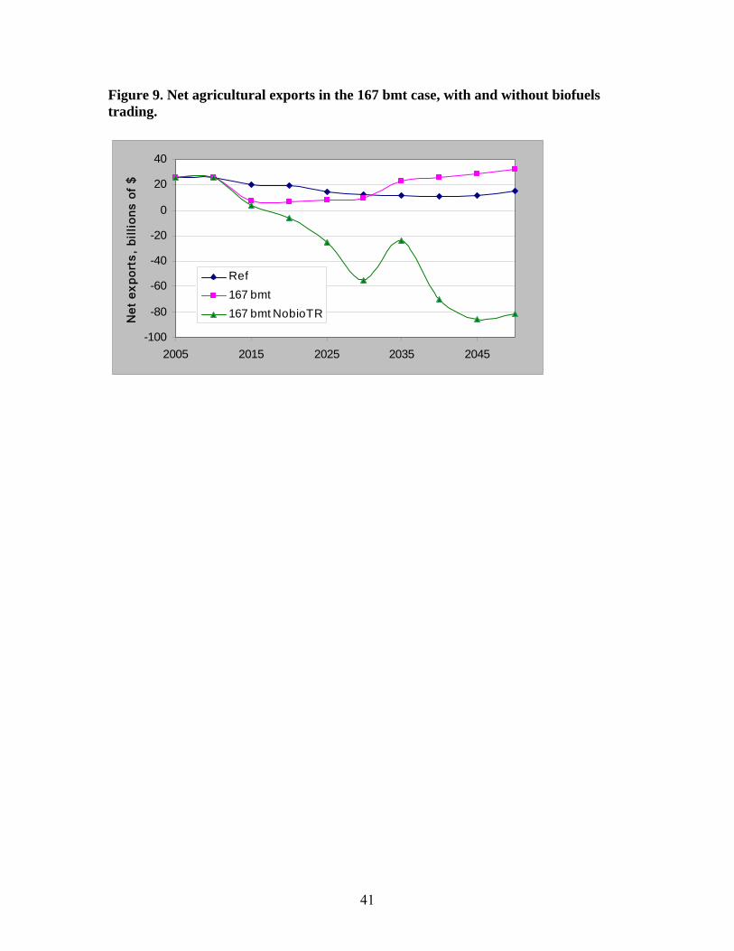
How is that possible and what are the implications for the broader agricultural sector?

Figure 9 illustrates one of the important implications of substantial biofuels production,

focusing on just the 167 bmt case. The US is currently a substantial net agricultural

exporter, and under the EPPA reference without GHG policy this is projected to continue.

In the 167 bmt case, USA net agricultural exports are projected to double compared with

19

a reference case without any policy. As other regions expand ethanol production, they

import more agricultural goods and thus USA net exports grow. The effect of forcing

biofuels to be produced domestically under a stringent climate policy is significant

reduction in USA agricultural production. Instead of the USA being a significant net

exporter of agricultural commodities, it becomes a large net importer. Whereas net

exports today are on the order of $20 billion, by 2050 in the 167 bmt NobioTR case the

USA grows to be a net importer of nearly $80 billion of agricultural commodities. The

agricultural sector in the EPPA model is highly aggregated—a single sector includes

crops, livestock, and forestry. As a result, one should not put too much stock in the

absolute value of net exports in the reference—it could be higher or lower depending on

how agricultural productivity advances in the USA relative to other regions of the world.

However, if about 25 EJ of ethanol must be produced in the USA (requiring about 500

million acres of land), it is nearly inevitable that this would lead to the USA becoming a

substantial agricultural importer.

Figure 10 shows an index of the land price, agricultural commodity price, and

agricultural production in the US relative to the reference in the 167 bmt NobioTR case.

Notably, agricultural land prices fall in 2015 relative to the reference, while agricultural

product prices rise. This reflects greenhouse gas mitigation costs in agriculture that

slightly depress land prices and agricultural production while leading to overall higher

production costs and agricultural prices. Agriculture uses a significant amount of energy

which emits CO2, and is also a significant source of N2O and CH4. The CO2-e price in

2015 in the 167 bmt NobioTR case is $67, and this added cost is reflected in a

combination of lower land prices and higher commodity prices determined by underlying

demand and supply elasticities. Once biofuels production increases, land prices recover

relative to the reference, agricultural commodity prices rise further, and agricultural

production falls further. The large shock in 2035 reflects the significant tightening of the

carbon constraint in developing countries in that year. The US reduces biofuel production

and imports petroleum. As a result, the land price temporarily is reduced though remains

above the reference.

20

Several other critical aspects of this level of biofuels production are worth pointing out.

Following the design of USA policies under consideration as well as policy design

discussion abroad such as the European emissions trading scheme or under the Kyoto

Protocol, we have not extended the cap and trade system to cover land use emissions (see

Reilly and Asadoorian, 2007). If included at all, land use is often covered under a

crediting system. However, as shown by McCarl and Reilly (2006), except for quite low

carbon prices, the economics of biofuels tends to dominate the economics of carbon

sequestration in soils. The implication is that at the level of biofuels demand simulated

here, there would be very little incentive to protect carbon in the soils and vegetation

through a credit system. Landowners would instead tend to convert land to biofuels or

more intense cropping. Whether the biofuels themselves are produced on existing

cropland or not, the overall need for cropland would require significant conversion of

land from less intensively managed grass and forestland. This initial disruption would

lead to significant carbon dioxide release from soils and vegetation. If mature forests are

converted it can take decades of biofuels production to make up for the initial carbon

loss. Whether this land is converted in the USA or somewhere abroad, it is likely to

contribute substantial carbon emissions, negating the savings from reduced fossil energy

use. Thus, one of the most serious issues raised in this analysis is the need to expand a

cap and trade system to include land use change emissions, and to be doubly concerned

about leakage from reductions in the USA through biofuels imports unless mitigation

policies abroad that include land use emissions are in place.

5. CONCLUSION

Two technologies which use biomass: electricity production from biomass and a liquid

fuel from biomass – are introduced into the EPPA model to estimate the biomass energy

use in different economic scenarios. Biomass technologies use land and a combination of

capital, labor and other inputs. They compete for land with other agricultural sectors. Our

approach represents biomass production, transportation, and conversion in a single

production function that we can benchmark to agro-engineering data on biomass

21

productivity per hectare and the cost and conversion efficiency of bio liquids and biomass

based electricity. A more structurally realistic treatment might represent explicitly

growing a crop for biomass (or several different crops), transportation of biomass to a

processing/conversion facility, conversion, and different end-use equipment

requirements. In our approach, we have no direct conventional energy inputs in this

process. We assume that the majority of needed energy (for harvesting/planting crop;

transporting to conversion facility, and in conversion) is provided by biomass itself, thus

we assume a relatively low (40%) conversion efficiency. Indirectly, other energy is used

in production of other industry/capital goods production that are inputs to bioenergy

production. We thus have no carbon emissions from bioenergy production itself.

Implicitly, we assume that biomass crops are grown in a “sustainable” manner in the

sense that CO2 released, when the bioenergy is produced and used, is taken up by the

next biomass crop. Given the potential scale of the bioenergy industry in the scenarios we

considered, this is unlikely to be a realistic assumption. Further modeling is needed to

investigate the potential carbon release from large scale land conversions that would be

needed to support a substantial bioenergy industry.

We test our representation of biomass technologies in different scenarios. Global increase

in biomass production in a reference scenario (with no climate change policy) is about 30

EJ/year by 2050 and about 180 EJ/year by 2100. This deployment is driven primarily by

a world oil price that in the year 2100 is over 4.5 times the price in the year 2000.

Different scenarios of stabilization of greenhouse gases increase the global biomass

production to 40-150 EJ/year by 2050 and 220-250 EJ/year by 2100. The area of land

required to produce 180-250 EJ/year is about 2Gha, an equivalent of the current global

total crop area. The magnitude and geographical distribution of climate-induced changes

may affect human’s ability to expand food production in order to feed growing

population. In addition to food production, consumption behavior might also shift in the

future with unexpected consequences. In another set of policy experiments we examine

the potential role of bioenergy in contributing to USA GHG mitigation efforts. We find a

substantial role for bioenergy but the USA, at least in our representation, imports biofuels

rather than grow them domestically. USA agriculture still expands because the need for

22

land for bio-fuels production abroad means that agricultural production is reduced

abroad, increasing USA agricultural exports. If we restrict USA biofuels to those

produced domestically, as much as 500 million acres of land would be required in the

USA for biofuels production, which would be enough to supply about 55% of the

country’s liquid fuel requirements. The result would be that the USA would need to

become a substantial agricultural importer, and this is further exaggerated if the rest of

world does not pursue a policy because then world food prices are lower because there is

less demand for biofuels abroad. This suggests that the idea that biomass energy

represents a significant domestic energy resource in the USA is misplaced. If the USA

were to actually produce a substantial amount of biofuels domestically through polices

that spurred its use but that prevented imports, instead of relying on oil imports the

country would need to rely on food imports. The overall conclusion is that the scale of

energy use in the USA and the world relative to biomass potential is so large that a

biofuel industry that was supplying a substantial share of liquid fuel demand would have

very significant effects on land use and conventional agricultural markets.

23

6. REFERENCES Babiker, M.H., G.E. Metcalf and J. Reilly (2003). “Tax distortions and global climate

policy”, Journal of Environmental Economics and Management, 46, 269-287. Brinkman, N., M. Wang, T. Weber, T. Darlington (2006). Well to Wheels Analysis of

Transportation Fuel Alternatives, Argonne National Lab. (http://www.transportation.anl.gov/pdfs/TA/339.pdf)

Climate Change Science Program (CCSP) (2006). CCSP Synthesis and Assessment

Product 2.1, Part A: Scenarios of Greenhouse Gas Emissions and Atmospheric Concentrations, L. Clarke et al., US Climate Change Science Program, Draft for CCSP Review, December 06, 2006.

Dimaranan B. and R. McDougall (2002). Global Trade, Assistance, and Production: The

GTAP 5 Data Base. Center for Global Trade Analysis, Purdue University, West Lafayette, Indiana.

Edmonds, J.A. and J. Reilly (1985). Global Energy: Assessing the Future, Oxford

University Press, New York. Energy Information Administration (EIA) (2006a). Emissions of Greenhouse Gases in

the United States 2005, Energy Information Administration, US Department of Energy, Washington DC.

Energy Information Administration (EIA) (2006b). International Energy Outlook 2006,

Energy Information Administration, U.S. Department of Energy, Washington, DC. Fedoroff, N. and J. Cohen (1999). Plants and Populations: Is There Time? Proceedings

of the National Academy of Sciences, USA, 96, 5903-5907. Fisher, G. and L. Schrattenholzer (2001). “Global Bioenergy Potentials through 2050”,

Biomass and Bioenergy, 20(3), 151-159. Frondel, M. and J. Peters (2007). “Biodiesel: A New Oildorado?”, Energy Policy, 35,

1675-1684. Hall, D., and F. Rosillo-Calle (1998). Biomass Resources other than Wood, World

Energy Council, London. Hamelinck, C., G. van Hooijdonk, and A. Faaij (2005). “Ethanol from lignocellulosic

biomass: techno-economic performance in short-, middle-, and long-term”, Biomass and Bioenergy, 28(4), 384-410.

Hertel, T. (1997). Global Trade Analysis: Modeling and Applications. Cambridge

University Press, Cambridge, UK.

24

Hill, J., E. Nelson, D. Tilman, S. Polasky and D. Tiffany (2006). Environmental,

economic, and energetic costs and benefits of biodiesel and ethanol biofuels. Proc. Natl. Acad. Sci. USA, 103, 11206-11210.

International Energy Agency (IEA) (1997). Renewable Energy Policy in IEA countries,

Volume II: Country reports, OECD/IEA, Paris. International Energy Agency (IEA) (2001). Answers to Ten Frequently Asked Questions

About Bioenergy, Carbon Sinks and Their Role in Global Climate Change, International Energy Agency, IEA Biomass Task 38, Greenhouse Gas Balances of Biomass and Bioenergy Systems, Paris, France. (http://www.ieabioenergy-task38.org/publications/faq/)

IPCC (2000). Land-Use, Land-Use Change, and Forestry, Special Report of the

Intergovernmental Panel on Climate Change, R. Watson et al (eds.), Cambridge University Press, UK.

IPCC (2001). Climate Change 2001: Mitigation, Contribution of Working Group III to

the Third Assessment Report of the Intergovernmental Panel on Climate Change, B. Metz et al (eds.), Cambridge University Press, UK.

Jacoby, H.D., R.S. Eckhaus, A.D. Ellerman, R.G. Prinn, D.M. Reiner and Z. Yang

(1997). “CO2 emissions limits: economic adjustments and the distribution of burdens,” The Energy Journal, 18(3), 31-58.

Jacoby, H.D., J. Reilly, J. McFarland and S. Paltsev (2006). “Technology and technical

change in the MIT EPPA model,” Energy Economics, 28, 610-631. McCarl, B. and J. Reilly (2006). Agriculture in the climate change and energy price

squeeze: Part 2: Mitigation Opportunities, Manuscript, Texas A&M, Department of Agricultural Economics.

McFarland, J, J. Reilly, and H.J. Herzog (2004). Representing Energy Technologies in

Top-Down Economic Models Using Bottom-Up Information, Energy Economics, 26, 685-707.

Moreira, J. R. (2004). Global Biomass Energy Potential, Paper prepared for the Expert

Workshop on Greenhouse Gas Emissions and Abrupt Climate Change, Paris 30 Sept.-1 Oct., manscript, Brazilian Reference Center on Biomass, Rua Francisco Dias Vlho, 814-04581.001, Sao Paulo, Brazil

Obersteiner M., C. Azar, K. Mollerstern, K. Riahi (2002). Biomass Energy, Carbon

Removal and Permanent Sequestration – A “Real Option” for Managing Climate Risk, IIASA Interim Report IR-02-042, International Institute for Applied Systems Analysis, Laxenburg, Austria.

25

Paltsev, S., J. Reilly, H.D. Jacoby, A.D. Ellerman and K.H. Tay (2003). Emissions

trading to reduce greenhouse gas emissions in the United States: The McCain-Lieberman Proposal. MIT Joint Program on the Science and Policy of Global Change, Report 97, Cambridge, MA. (http://web.mit.edu/globalchange/www/MITJPSPGC_Rpt97.pdf).

Paltsev, S., H. Jacoby, J. Reilly, L. Viguier and M. Babiker (2004). Modeling the

Transport Sector: The Role of Existing Fuel Taxes in Climate Policy, MIT Joint Program on the Science and Policy of Global Change, Report 117, Cambridge, MA. (http://web.mit.edu/globalchange/www/MITJPSPGC_Rpt117.pdf).

Paltsev, S., J. Reilly, H. Jacoby, R. Eckaus, J. McFarland, M. Sarofim, M. Asadoorian,

and M. Babiker (2005). The MIT Emissions Prediction and Policy Analysis (EPPA) Model: Version 4, MIT Joint Program on the Science and Policy of Global Change, Report 125, Cambridge, MA. (http://web.mit.edu/globalchange/www/MITJPSPGC_Rpt125.pdf).

Paltsev, S., J. Reilly, H. Jacoby, A. Gurgel, G. Metcalf, A. Sokolov and J. Holak (2007). Assessment of US Cap-and-Trade Proposals, MIT Joint Program on the Science and Policy of Global Change, Report 146, Cambridge, MA (http://web.mit.edu/globalchange/www/MITJPSPGC_Rpt146.pdf).

Reilly, J. and M. Asadoorian (2007). “Mitigation of Greenhouse Gas Emissions from Land Use: Creating Incentives within Greenhouse Gas Emissions Trading Systems,” Climatic Change, 80,173–197.

Reilly, J. and K. Fuglie (1998). “Future Yield Growth in Field Crops: What Evidence

Exists?” Soil and Tillage Research, 47, 275-290. Reilly, J., Prinn, R.,J. Harnisch, J. Fitzmaurice, H. Jacoby, D. Kicklighter, J. Melillo, P.

Stone, A. Sokolov and C. Wang (1999). “Multi-gas assessment of the Kyoto Protocol,” Nature, 401, 549-555.

Reilly, J. and S. Paltsev (2006). “European Greenhouse Gas Emissions Trading: A System in Transition,” in Economic Modeling of Climate Change and Energy Policies, M. De Miguel, X. Labandeira, B. Manzano (eds.), 2006, Edward Elgar Publishing, 45-64.

Reilly, J., S. Paltsev, B. Felzer, X. Wang, D. Kicklighter, J. Melillo, R. Prinn, M.

Sarofim, A. Sokolov, C. Wang (2007). “Global Economic Effects of Changes in Crops, Pasture, and Forests due to Changing Climate, Carbon Dioxide, and Ozone”, Energy Policy, forthcoming.

Rimmer, M.T. and A.A. Powell (1996). “An implicitly, directly additive demand

system,” Applied Economics, 28, 1613-1622.

26

Rutherford, T. (1995). Demand Theory and General Equilibrium: An Intermediate Level

Introduction to MPSGE, GAMS Development Corporation, Washington, DC. (http://www.gams.com/solvers/mpsge/gentle.htm)

Smeets, E. and A. Faaij (2007). “Bioenergy Potentials from Forestry in 2050: An Assessment of the Drivers that Determine the Potentials”, Climatic Change, 81, 353-390.

27

Table 1. World Land Area and a Potential for Energy from Biomass

Area, Gha

max dry bioenergy, EJ

max liquid bioenergy, EJ

Tropical Forests 1.76 528 211 Temperate Forests 1.04 312 125 Boreal forests 1.37 411 164 Tropical Savannas 2.25 0 0 Temperate grassland 1.25 375 150 Deserts and Semideserts 4.55 0 0 Tundra 0.95 0 0 Wetlands 0.35 0 0 Croplands 1.60 480 192 Total 15.12 2106 842

Source: area (IPCC, 2000); assumptions about area to energy conversion – 15 odt/ha/year and 20 GJ/odt (IPCC, 2001); assumption for conversion efficiency from biomass to liquid energy product – 40%.

28

Table 2. U.S. Land Area and a Potential for Energy from Biomass

Area, Gha

Area, billion acres

max dry bioenergy, EJ

max liquid bioenergy, EJ

Cropland 0.177 0.442 53.0 21.2 Grassland 0.235 0.587 70.4 28.2 Forest 0.260 0.651 78.1 31.2 Parks, etc 0.119 0.297 0 0 Urban 0.024 0.060 0 0 Deserts, Wetland, etc 0.091 0.228 0 0 Total 0.906 2.265 201.6 80.6

Source: area (USDA, 2005); assumptions about area to energy conversion – 15 odt/ha/year and 20 GJ/odt (IPCC, 2001); assumption for conversion efficiency from biomass to liquid energy product – 40%.

29

Table 3. Regions and Sectors in the EPPA4 Model Country/Region Sectors _______________________________________________________________ Annex B Non-Energy United States (USA) Agriculture (AGRI) Canada (CAN) Services (SERV) Japan (JPN) Energy Intensive Products (EINT) European Union+ (EUR) Other Industries Products (OTHR) Australia/New Zealand (ANZ) Industrial Transportation (TRAN) Former Soviet Union (FSU) Household Transportation (HTRN) Eastern Europe (EET) Energy Non-Annex B Coal (COAL) India (IND) Crude Oil (OIL) China (CHN) Refined Oil (ROIL) Indonesia (IDZ) Natural Gas (GAS) Higher Income East Asia (ASI) Electric: Fossil (ELEC) Mexico (MEX) Electric: Hydro (HYDR) Central and South America (LAM) Electric: Nuclear (NUCL) Middle East (MES) Advanced Energy Technologies Africa (AFR) Electric: Biomass (BELE) Rest of World (ROW) Electric: Natural Gas Combined Cycle (NGCC)

Electric: NGCC with CO2 Capture and Storage (NGCAP) Electric: Integrated Coal Gasification with

CO2 Capture and Storage (IGCAP) Electric: Solar and Wind (SOLW)

Liquid fuel from biomass (BOIL) Oil from Shale (SYNO)

Synthetic Gas from Coal (SYNG) Note: Detail on the regional composition is provided in Paltsev et al. (2005). AGRI, SERV, EINT, OTHR, COAL, OIL, ROIL, GAS sectors are aggregated from the GTAP data (Dimaranan and McDougall, 2002), TRAN and HTRN sectors are disaggregated as documented in Paltsev et al. (2004), ELEC, HYDR and NUCL are disaggregated from electricity sector (ELY) of the GTAP dataset based on EIA data (2006b), BELE, NGCC, NGCAP, IGCAP, SOLW, BOIL, SYNO, SYNG sectors are advanced technology sectors that do not exist explicitly in the GTAP dataset.

30

Table 4. Mark-ups and Input Shares for Bio-oil and Bio-electric Technologies Supply Technology

Mark-up Factor

Input Shares Resource OTHR Capital Labor Fixed Factor

Bio-oil 2.1 0.10 0.18 0.58 0.14 -- Bio-electric 1.4-2.0 0.19 0.18 0.44 0.14 0.05

31

Table 5. Reference Values for Elasticities in Bio-oil and Bio-electric Technologies

σRVA Resource-Value Added/Other 0.3

0.1

Bio-Electric

Bio-oil

σFVA Fixed Factor-Value Added/Other 0.4 Bio-Electricity

σVAO Labor-Capital-OTHR 1.0 Bio-oil & Bio-Electricity

32

Table 6. US land area (Mha) required for biomass production in CCSP scenarios 2010 2020 2030 2040 2050 2060 2070 2080 2090 2100 ref 11 5 16 48 50 61 91 114 131 147 Level 4 11 5 21 49 63 96 132 155 175 158 Level 3 11 5 25 51 82 128 166 191 179 170 Level 2 11 6 41 79 175 238 237 200 198 187 Level 1 11 56 144 253 272 261 251 226 202 174 Table 7. Global land area (Mha) required for biomass production in CCSP scenarios 2010 2020 2030 2040 2050 2060 2070 2080 2090 2100 ref 46 27 88 261 281 346 496 601 672 728 Level 4 46 27 115 267 341 501 663 752 857 942 Level 3 46 29 134 271 422 619 753 868 987 1011 Level 2 46 30 209 391 739 933 1070 1117 1071 1002 Level 1 46 268 589 958 1229 1264 1208 1122 1032 921 Table 8. US land area (Mha) required for biomass production in US Congressional analysis scenarios

2015 2020 2025 2030 2035 2040 2045 2050 287 bmt 0 0 0 0 0 0 0 0 287 bmt NobioTR 0 0 0 0 0 0 0 1 203 bmt 0 0 0 0 0 0 0 4 203 bmt NobioTR 5 3 2 60 1 71 165 239 167 bmt 0 0 0 0 0 0 0 6 167 bmt NobioTR 5 44 116 202 155 246 268 260

Table 9. Global land area (Mha) required for biomass production in US Congressional analysis scenarios

2015 2020 2025 2030 2035 2040 2045 2050 287 bmt 0 0 58 185 642 751 827 880 287 bmt NobioTR 0 0 9 80 502 603 695 770 203 bmt 5 13 115 297 622 763 944 1057 203 bmt NobioTR 5 3 11 123 496 656 834 981 167 bmt 5 85 230 377 760 905 1001 1059 167 bmt NobioTR 5 44 124 246 627 808 924 996

33

Figure 1. Structure of Biotechnology Production Functions Panel a. Bio-oil

Panel b. Bio-electric

Electricity Output

Resource(Land)

Value-Added &Intermediates

OTHR Capital Labor

Fixed Factor

σVAO

σFVA

σ RVA

σ

Labor

σ

σ VAO

RVA

CapitalOTHR

Resource (Land)

Value-Added &Intermediates

Refined Oil (ROIL) Substitute

34

Figure 2. Global Biomass Production across Scenarios

0

50

100

150

200

250

300

2000 2020 2040 2060 2080 2100

year

EJ

/ye

ar

refLevel 4Level 3Level 2Level 1

35

Figure 3. U.S. Biomass Production across Scenarios

05

101520253035404550

2000 2020 2040 2060 2080 2100

year

EJ

/ye

ar

refLevel 4Level 3Level 2Level 1

36

Figure 4. Global Primary Energy Consumption in the reference

Global Primary Energy: Reference

0

200

400

600

800

1 000

1 200

1 400

1 600

2000 2010 2020 2030 2040 2050 2060 2070 2080 2090 2100

Year

Exaj

oule

s/Ye

ar

Non-Biomass Renew ablesNuclearCommercial BiomassCoalNatural GasOil

37

Figure 5. Global Primary Energy in the Level 3 Scenario

Global Primary Energy: Level 3

0

200

400

600

800

1,000

1,200

1,400

1,600

2000 2010 2020 2030 2040 2050 2060 2070 2080 2090 2100Year

Exaj

oule

s/Ye

ar

Energy Reduction from ReferenceNon-Biomass Renew ablesNuclearCommercial BiomassCoal: w / CCSCoal: w /o CCSNatural Gas: w / CCSNatural Gas: w /o CCSOil: w / CCSOil: w /o CCS

38

Figure 6. Global Primary Energy in the Level 1 Scenario

Global Primary Energy: Level 1

0

200

400

600

800

1,000

1,200

1,400

1,600

2000 2010 2020 2030 2040 2050 2060 2070 2080 2090 2100Year

Exaj

oule

s/Ye

ar

Energy Reduction from ReferenceNon-Biomass Renew ablesNuclearCommercial BiomassCoal: w / CCSCoal: w /o CCSNatural Gas: w / CCSNatural Gas: w /o CCSOil: w / CCSOil: w /o CCS

39

Figure 7. Land Price and Agriculture Output Price in USA in the Level 2 Scenario compared with the Reference Prices

0.00

0.50

1.00

1.50

2.00

2.50

2000 2020 2040 2060 2080 2100

Ind

ex

, R

ef

pri

ce

= 1

Land Price

AgricultureOutput Price

40

Figure 8. Liquid biofuel use, with and without international trade in biofuels. Panel a. USA

0

5

10

15

20

25

30

35

40

2015 2020 2025 2030 2035 2040 2045 2050

Us

e (

EJ

)

287 bmt

287 bmt NobioTR

203 bmt

203 bmt NobioTR

167 bmt

167 bmt NobioTR

Panel b. World Total

0

20

40

60

80

100

120

140

2015 2020 2025 2030 2035 2040 2045 2050

Us

e (

EJ

)

287 bmt

287 bmt NobioTR

203 bmt

203 bmt NobioTR

167 bmt

167 bmt NobioTR

41

Figure 9. Net agricultural exports in the 167 bmt case, with and without biofuels trading.

-100

-80

-60

-40

-20

0

20

40

2005 2015 2025 2035 2045

Ne

t e

xp

ort

s,

bil

lio

ns

of

$

Ref167 bmt167 bmt NobioTR

42

Figure 10. Indexes of Agriculture Output Price, Land Price, and Agriculture Production in USA in No Biofuel Trading (167bmtNB) Scenario Relative to the Reference (2010 = 1.00)

00.2

0.40.6

0.81

1.2

1.41.6

1.82

2010 2020 2030 2040 2050

Ind

ex

(20

10

=1

)

Agriculture Output Price

Land Price

Agriculture Production