biological monitoring quality control - advisory committee on water

4

Partitioning Error Sources for Quality Control and Comparability Analysis in Biological

Monitoring and Assessment

James B. Stribling Tetra Tech, Inc., Center for Ecological Sciences,

Owings Mills, Maryland USA

“…measurements are not passive accountings of an objective world but active interactions in which the thing measured and the way it is measured contribute inseparably to the

outcome.” (Lindley 2007: p. 154, attributing the concept to Neils Bohr)

“The experienced scientist has to learn to anticipate the possible sources of systematic error...” (Taylor 1997: p. 97)

“No simple theory tells us what to do about systematic errors. In fact, the only theory of systematic errors is that they must be identified and reduced....” (Taylor 1997: p. 106)

“…the only reason to carry out a test is to improve a process, to improve the quality...” (Deming 1986: p. i)

1. Introduction

Rationally, as scientists, we recognize that documented standard procedures constitute the first requirement for developing consistency within and among datasets; the second step is putting the procedures into practice. If the procedures were implemented as perfectly as they are written, there would be no need to question data. However, we are also cognizant of the fact that humans (a group of organisms to which we cannot deny holding membership) are called upon to use the procedures, and the consistency and rigor with which the procedures are applied are directly affected by an individual’s skill, training, attention span, energy, and focus (Edwards, 2004). In fact, we fully expect inconsistency due to human foibles, and often substantial portions of careers are spent in efforts to recognize, isolate, correct, and minimize future occurrences of, error. Many public and private organizations in the United States (US) and other countries collect aquatic biological data using a variety of sampling and analysis methods (Gurtz & Muir, 1994; ITFM, 1995a; Carter & Resh, 2001), often for meeting regulatory requirements, for example, by the United States’ Clean Water Act (CWA) of 1972 (USGPO, 1989). While the information collected by an individual organization is usually directly applicable to a specific question or site-specific issue, the capacity for using it more broadly for comprehensive assessment has been problematic due to unknown data quality produced by different methods or programs (ITFM, 1995a; Diamond et al., 1996; NWQMC, 2001; The

(for citation information, see bottom of last page)

Modern Approaches To Quality Control

60

Heinz Center, 2002; GAO, 2004). If the occurrence and magnitude of error in datasets is unknown, a supportable conclusion based solely (or even in part) on those data is problematic at best. These datasets are more difficult to justify for analyses, communicate to broader audiences, base policy decisions on, and defend against potential misuse (Costanza et al., 1992; Edwards, 2004). To ensure the measurement system produces data that can be defended requires understanding the potential error sources that can affect variability of the data and approaches for monitoring the magnitude of error expression. The purpose of this chapter is to communicate the concept of biological monitoring and assessment as a series of methods, each of which produces data and are as subject to error as any other measurement system. It will describe specific QC techniques and analyses that can be used to monitor variability (i.e., error), identify causes, and develop corrective actions to reduce or otherwise control error rates within acceptable limits. The chapter concludes by demonstrating that comparability analysis for biological data and assessment results is a two-step process, including 1) characterizing data quality, or the magnitude of error rates, associated with each method or dataset, and 2) determining acceptability. It should also be recognized that specific methods are not recommended in the chapter, but rather, emphasis is given that whatever methods are used, data quality and performance should be quantified. Additionally, special emphasis is given to biological monitoring where benthic macroinvertebrate sampling provides the primary data, but conceptually, this approach to QC is also applicable to other organism groups.

2. Quality control

Quality control (QC) is a process by which tests are designed and performed to document the existence and causes of error (=variability) in data, as well as helping determine what can be done to minimize or eliminate them, and developing, communicating, and monitoring corrective actions (CA). Further, it should also be possible to implement the QC process (Figure 1) in a routine manner such that, when those causes are not present, the cost of searching for them does not exceed budgetary constraints (Shewhart, 1939).

Fig. 1. Quality control (QC) process for determining the presence of and managing error rates, and thus, the acceptability of data quality.

Partitioning Error Sources for Quality Control and Comparability Analysis in Biological Monitoring and Assessment

61

The programmatic system that contains not only a series of QC tests and analyses, but also provides for organization and management of personnel, acquisition and maintenance of equipment and supplies essential to data collection, information management, information technology resources, safety protocols and facilities, enforcement of corrective actions, and budgetary support, is quality assurance (QA). It is acceptable to use the two terms jointly in reference to an overall quality program, as they often are, as QA/QC, but they should not be used interchangeably. The overall program is QA; the process for identifying and reducing error is QC. Overall variability of data (= total uncertainty, or error) from any measurement system results from accumulation of error from multiple sources (Taylor 1988; Taylor & Kuyatt, 1994; Diamond et al., 1996; Taylor, 1997). Error can generally be divided into two types: systematic and random. Systematic error is the type of variability that results from a method and its application or mis-application; it is composed of bias that can, in part, be mediated by using an appropriate quality assurance program of training, audits, and documentation. Random error results from the sample itself or the population from which it is derived, and can only partly be controlled through a careful sampling design. It is often not possible to separate the effects of the two types of error, and they can directly influence each other (Taylor, 1988). The overall magnitude of error associated with a dataset is known as data quality; how statements of data quality are made and communicated are critical for data users and decision makers to properly evaluate the extent to which they should rely on technical, scientific, information (Keith, 1988; Peters, 1988; Costanza et al., 1992). Thus, an effective set of QC procedures helps not only reduce error in datasets, it provides tools for objective communication of uncertainty. Biological assessment protocols are measurement systems consisting of a series of methods, each of which contribute to overall variability (Diamond et al., 1996; Cao et al., 2003; Brunialti et al., 2004; Flotemersch et al., 2006; Haase et al., 2006; Nichols et al., 2006; Blocksom & Flotemersch, 2008) (Figure 2). Our capacity as practitioners to control rates and magnitudes of error requires some attention be given to each component of the protocol. While it could be argued that error arising from any single component has only trivial effects on the overall indicator, lack of testing and documentation can substantially weaken that assertion, and opens the results to question. In fact, information without associated data quality characteristics might not even be considered data.

Fig. 2. Total error or variability (s2) associated with a biological assessment is a combined result of that for each component of the process (Flotemersch et al. 2006).


62

3. Indicators

All aquatic ecosystems are susceptible to cumulative impacts from human-induced disturbances including inorganic and organic chemical pollution, hydrologic alteration, channelization, overharvest, invasive species, and land cover conversion. Because they live in the presence of existing water chemistry and physical habitat conditions, the aquatic life of these systems (fish, insects, plants, shellfish, amphibians, reptiles, etc.) integrates cumulative effects of multiple stressors that are produced by both point and non-point source (NPS) pollution. The most common organism groups that are used by routine biological monitoring and assessment programs are benthic macroinvertebrates (aquatic insects, snails, mollusks, crustaceans, worms, and mites), fish, and/or algae, with indicators most often taking the form of a multimetric Index of Biological Integrity (IBI; Karr et al., 1986; Hughes et al., 1998; Barbour et al., 1999; Hill et al., 2000, 2003) or a predictive observed/expected (O/E) model based on the River Invertebrate Prediction and Classification System (RIVPACS; Clarke et al., 1996, 2003; Hawkins et al., 2000; Hawkins, 2006). Of these latter three groups, benthic macroinvertebrates (BM) are commonly used because the protocols are most well-established, the level of effort required for field sampling is reasonable (Barbour et al., 1999), and taxonomic expertise is relatively easily accessible. Thus, examples of QC tests and corrective actions discussed in this chapter are largely focused on benthic macroinvertebrates in the context of multimetric indexes, though, similar procedures for routine monitoring with algae and fish could be developed. Stribling et al. (2008) also used some of these procedures for documenting performance of O/E models.

4. Potential error sources in indicators

4.1 Field sampling Whether the target assemblage is benthic macroinvertebrates, fish, or algae, the first step of biological assessment is to use standard field methods to gather a sample representing the taxonomic diversity and functional composition of a reach, zone, or other stratum of a waterbody. The actual dimensions of the sampling area ultimately depend on technical objectives and programmatic goals of the monitoring activity (Flotemersch et al., 2010). The spatial area from which the biological sample is drawn is that segment or portion of the waterbody the sample is intended to represent; for analyses and higher level interpretation, biological indicators are considered equivalent to the site. For its national surveys of lotic waters (streams and rivers), the U. S. Environmental Protection Agency defines a sample reach as 40x the mean wetted width (USEPA, 2004a); many individual states use a fixed 100m as the sampling reach. Benthic macroinvertebrate samples are collected along 11 transects evenly distributed throughout the reach length, and a D-frame net with 500-µm mesh openings used to sample multiple habitats (Klemm et al., 1998; USEPA, 2004a; Flotemersch et al., 2006). An alternative approach to transects is to estimate the proportion of different habitat types in a defined reach (e.g., 100m), and distribute a fixed level of sampling effort in proportion to their frequency of occurrence throughout the reach (Barbour et al., 1999, 2006). For both approaches, organic and inorganic sample material (leaf litter, small woody twigs, silt, and sand) are composited in one or more containers, preserved with 95% denatured ethanol, and delivered to laboratories for processing. A composite sample over multiple habitats in a reach is a common protocol feature of many monitoring program throughout the US (Carter & Resh, 2001).


63

4.2 Laboratory processing Processing of benthic macroinvertebrate samples is a 3-step process. Sorting and subsampling serves to 1) isolate individual organisms from nontarget material, such as leaf litter and other detritus, bits of woody material, silt, and sand, and 2) prepare the sample (or subsample) for taxonomic identification. Taxonomic identification serves to match nomenclature to specimens in the sample, and enumeration provides the actual counts, by taxon, of everything contained within the sample. Although it is widely recognized that subsampling helps to manage the level of effort associated with bioassessment laboratory work (Carter & Resh, 2001), the practice has been the subject of much debate (Courtemanch, 1996; Barbour & Gerritsen, 1996; Vinson & Hawkins, 1996). Fixed organism counts vary among monitoring programs (Carter & Resh, 2001), with 100, 200, 300 and 500 counts being most often used (Barbour et al., 1999; Cao & Hawkins, 2005; Flotemersch et al., 2006). Flotemersch & Blocksom (2005) concluded that a 500-organism count was most appropriate for large/nonwadeable river systems, based on examination of the relative increase in richness metric values (< 2%) between successive 100-organism counts. However, they also suggested that 300-organism count is sufficient for most study needs. Others have recommended higher fixed counts, including a minimum of 600 in wadeable streams (Cao & Hawkins, 2005). The subsample count used for the USEPA national surveys is 500 organisms (USEPA, 2004b); many states use 200 or 300 counts. If organisms are missed during the sorting process, bias is introduced in the resulting data. Thus, the primary goal of sorting is to completely separate organisms from organic and inorganic material (e.g., detritus, sediment) in the sample. A secondary goal of sorting is to provide the taxonomist with a sample for which the majority of specimens are identifiable. Note that the procedure described here assumes that the sorter and the taxonomist are different personnel. Although it is not the decision of the sorter whether an organism is identifiable, straightforward rules can be applied that minimize specimen loss. For example, “counting rules” can be part of the standard operating procedures (SOP) for both the sorting/subsampling and taxonomic identification, such as specifying what not to count: Non-benthic organisms, such as free-swimming gyrinid adults (Coleoptera) or surface-

dwelling veliids (Heteroptera) Empty mollusk shells (Mollusca: Bivalvia and Gastropoda) Non-headed worm fragments Damaged insects and crustaceans that lack at least a head and thorax Incidental collections, such as terrestrial insects or aquatic vertebrates (fish, frogs or

tadpoles, snakes, or other) Non-macroinvertebrates, such as copepods, cladocera, and ostracods Exuviae (molted “skins”) Larvae or pupae where internal tissue has broken down to point of floppiness If a sorter is uncertain about whether an organism is countable, the specimen should be placed in the vial and not added to the rough count total. The sorting/subsampling process is based on randomly selecting portions of the sample detritus spread over a gridded Caton screen (Caton, 1991; Barbour et al., 1999; see also Figures 6-4a, b of Flotemersch et al., 2006 [note that an individual grid square is 6 cm x 6 cm, or 36 cm2, not 6 cm2 as indicated in Figure 6-4b]). Prior to beginning the sorting/subsampling process, it is important that the sample be mixed thoroughly and distributed evenly across the sorting tray to reduce the effect of organism clumping that may have occurred in the sample container. The grids are randomly selected, individually removed from the screen, placed in a sorting tray, and all organisms removed with forceps;


64

the process is completed until the rough count by the sorter exceeds the target subsample size. There should be at least three containers produced per sample, all of which should be clearly labeled: 1) subsample to be given to taxonomist, 2) sort residue to be checked for missed specimens, and 3) unsorted sample remains to be used for additional sorting, if necessary. The next step of the laboratory process is identifying the organisms within the subsample. A major question associated with taxonomy for biological assessments is the hierarchical target levels required of the taxonomist, including order, family, genus, species or the lowest practical taxonomic level (LPTL). While family level is used effectively in some monitoring programs (Carter & Resh 2001), the taxonomic level primarily used in most routine monitoring programs is genus. However, even with genus as the target, many programs often treat selected groups differently, such as midges (Chironomidae) and worms (Oligochaeta), due to the need for slide-mounting. Slide-mounting specimens in these two groups is usually (though, not always) necessary to attain genus level nomenclature, and sometimes even tribal level for midges. Because taxonomy is a major potential source of error in any kind of biological monitoring data sets (Stribling et al., 2003, 2008a; Milberg et al., 2008; Bortolus, 2008), it is critical to define taxonomic expectations and to treat all samples consistently, both by a single taxonomist and among multiple taxonomists. This, in part, requires specifying both hierarchical targets and counting rules. An example list of taxonomic target levels is shown in Table 1. These target levels define the level of effort that should be applied to each specimen. If it is not possible to attain these levels for certain specimens due to, for example, the presence of early instars, damage, or poor slide mounts, the taxonomist provides a more coarse-level identification. When a taxonomist receives samples for identification, depending upon the rigor of the sorting process (see above), the samples may contain specimens that either cannot be identified, or non-target taxa that should not be included in the sample. The final screen of sample integrity is the responsibility of the taxonomist, who determines which specimens should remain unrecorded (for any of the reasons stated above). Beyond this, the principal responsibility of the taxonomist is to record and report the taxa in the sample and the number of individuals of each taxon. Programs should use the most current and accepted keys and nomenclature. An Introduction to the Aquatic Insects of North America (Merritt et al., 2008) is useful for identifying the majority of aquatic insects in North America to genus level. By their very nature, most taxonomic keys are obsolete soon after publication; however, research taxonomists do not discontinue research once keys are available. Thus, it is often necessary to have access to and be familiar with ongoing research in different taxonomic groups. Other keys are also necessary for non-insect benthic macroinvertebrates that will be encountered, such as Oligochaeta, Mollusca, Acari, Crustacea, Platyhelminthes, and others. Klemm et al. (1990) and Merritt et al. (2008) provide an exhaustive list of taxonomic literature for all major groups of freshwater benthic macroinvertebrates. Although it is not current for all taxa, the integrated taxonomic information system (ITIS; http://www.itis.usda.gov/) has served as a clearinghouse for accepted nomenclature, including validity, authorship and spelling.

4.3 Data entry Taxonomic nomenclature and counts are usually entered into the data management system directly from handwritten bench or field sheets. Depending on the system used, there may be an autocomplete function that helps prevent misspellings, but which can also contribute to errors. For example, entering the letters ‘hydro’ could potentially autocomplete as either


65

Hydropsyche or Hydrophilus, and the data entry technician on autopilot might continue as normal. There are also, increasingly, uses of e-tablets for entering field observation data, or direct entry of laboratory data into spreadsheets, obviating the need for hardcopy paper backup.

4.4 Data reduction/indicator calculation There is a large number of potential metrics that monitoring programs can use (Barbour et al., 1999; Blocksom & Flotemersch, 2005; Flotemersch et al., 2006), requiring testing, calibration, and final selection before being appropriate for routine application. Blocksom & Flotemersch (2005) tested 42 metrics relative to different sampling methods, mesh sizes, and habitat types, some of which are based on taxonomic information, as well as stressor tolerance, functional feeding group, and habit. Other workers and programs have tested more and different ones. For example, the US state of Montana calibrated a biological indicator for wadeable streams of the “mountains” site class (Montana DEQ 2006), resulting in a multimetric index comprised of seven metrics (Table 2).

Taxon Target

Ceratopogonidae Ceratopogoninae, leave at subfamily; all others, genus level

Dolichopodidae (Dolichopodidae)Phoridae (Phoridae)

Scathophagidae (Scathophagidae)Syrphidae (Syrphidae)Decapoda FamilyHirudinea Family

Hydrobiidae (Hydrobiidae)Nematoda (Nematoda)

Nematomorpha (Nematomorpha)Nemertea (Nemertea)

Turbellaria (Turbellaria)Chironomidae, the following genera are combined under

Cricotopus/OrthocladiusCricotopus Cricotopus/Orthocladius

Orthocladius Cricotopus/OrthocladiusCricotopus/Orthocladius Cricotopus/OrthocladiusOrthocladius/Cricotopus Cricotopus/Orthocladius

Chironomidae, the following genera are combined under Thienemannimyia genus group

Conchapelopia Thienemannimyia genus groupRheopelopia Thienemannimyia genus groupHelopelopia Thienemannimyia genus groupTelopelopia Thienemannimyia genus groupMeropelopia Thienemannimyia genus groupHayesomia Thienemannimyia genus group

Thienemannimyia Thienemannimyia genus groupHydropsychidae, the following genera are combined under

HydropsycheHydropsyche HydropsycheCeratopsyche Hydropsyche

Hydropsyche/Ceratopsyche HydropsycheCeratopsyche/Hydropsyche Hydropsyche

Table 1. In this example list of hierarchical target levels, all taxa are targeted for identification to genus level, unless otherwise noted. Taxa with target levels in parentheses are left at that level.


66

This discussion assumes that the indicator terms have already been calibrated and selected, and deals specifically with their calculation. For this purpose, the raw data are taxa lists and counts; their conversion into metrics is data reduction usually performed with computer spreadsheets or in relational databases. To ensure that database queries are correct and result in the intended metric values, a subset of values should be recalculated by hand. One metric is calculated for all samples, all metrics are calculated for one sample. When recalculated values differ from those values in the matrix, the reasons for the disagreement are determined and corrections are made. Reports on performance include the total number of reduced values as a percentage of the total, how many errors were found in the queries, and the corrective actions specifically documented.

4.5 Indicator reporting Regardless of whether the indicator is based on a multimetric framework or multivariate predictive model, the ultimate goal is to translate the quantitative, numeric result, the score, into some kind of narrative that provides the capacity for broad communication. The final assessment for a site is usually determined based on a site score relative to the distribution of reference site scores to reflect degrees of biological degradation, the more similar a test site is to reference less degradation is being exhibited. Depending on the calibration process and how many condition categories are structured, narratives for individual sites can come from two categories (degraded, nondegraded), three (good, fair, poor), four (good, fair, poor, very poor), or five (very good, good, fair, poor, or very poor). There also may be other frameworks a program chooses to use, but the key is to have the individual categories quantitatively-defined.

Metric Description Number of Ephemeroptera taxa

Count of the number of distinct taxa of mayflies in sample

Number of Plecoptera taxa Count of the number of distinct taxa of stoneflies in sample

% individuals as EPT Percent of individuals in sample that is mayflies, stoneflies, or caddisflies (Ephemeroptera, Plecoptera, or Trichoptera, respectively)

% individuals as non-insects Percent of individuals in sample as non-insects % individuals as predators Percent of individuals in sample as predators % of taxa as burrowers Percent of taxa in sample as burrower habit

Hilsenhoff Biotic Index Abundance-weighted mean of stressor tolerance values for taxa in the sample

Table 2. Sample-based metrics calculated for benthic macroinvertebrates. Shown are those developed and calibrated for streams in the “mountains” site class of the state of Montana, USA (Montana DEQ 2006, Stribling et al. 2008b).

5. Measurement quality objectives (MQO)

For each step of the biological assessment process there are different performance characteristics that can be documented, some of which are quantitative and others that are qualitative (Table 3). Measurement quality objectives (MQO) are control points above (or


67

below) which most observed values fall (Diamond et al., 2006; Flotemersch et al., 2006; Stribling et al., 2003, 2008a, b; Herbst & Silldorf, 2006), and are roughly analogous to the Shewhart (1939) concept of process control.

Component method or activity

Performance characteristics

Pre

cisi

on

Acc

ura

cy

Bia

s

Rep

rese

nta

tive

nes

s

Com

ple

ten

ess

1. Field sampling na ∆ ∆ 2. Laboratory sorting/subsampling na ∆ 3. Taxonomy na na 4. Enumeration ∆ na 5. Data entry na na na 6. Data reduction (e. g., metric calculation) na ∆ na na

7. Site assessment and interpretation ∆ ∆ Table 3. Error partitioning framework for biological assessments and biological assessment protocols for benthic macroinvertebrates. There may be additional activities and performance characteristics, and they may be quantitative (), qualitative (∆) or not applicable (na).

Specific MQO should be selected based on the distribution of values attained, particularly the minima and maxima. Importantly, for environmental monitoring programs, special studies should never be the basis upon which a particular MQO is selected; rather, they should reflect performance expectations when routine techniques and monitoring personnel are used. Consider MQO that are established using data from the best field team, or the taxonomist with the most years of experience, or the dissolved oxygen measurements taken using the most expensive field probes. When those people or equipment are no longer available to the program, how useful would the database be to future or secondary users? Defensibility would potentially be diminished. Values that are >MQO are not automatically taken to be unacceptable data points; rather, such values are targeted for closer scrutiny to determine possible reasons for exceedence and might indicate a need for corrective actions (Stribling et al. 2003, Montana DEQ 2006). Simultaneously, they can be used to help quantify performance of the field teams in consistently applying the methods.

5.1 Field sampling Quantitative performance characteristics for field sampling are precision and completeness (Table 3). Repeat samples for purposes of calculating precision of field sampling are


68

obtained by sampling two adjacent reaches, shown as 500 m in this example (Figure 3), and can be done by the same field team for intra-team precision, or by different teams for inter-team precision. For benthic macroinvertebrates, samples from the adjacent reaches (also called duplicate or quality control [QC] samples) must be laboratory-processed prior to data being available for precision calculations. Assuming acceptable laboratory error, these precision values are statements of the consistency with which the sampling protocols 1) characterized the biology of the stream or river and 2) were applied by the field team, and thus, reflect a combination of natural variability and systematic error inherent in the dataset.

Fig. 3. Adjacent reaches (primary and repeat) for calculating precision estimates (Flotemersch et al. 2006).

The number of reaches for which repeat samples are taken varies, but a rule-of-thumb is 10%, randomly-selected from the total number of sampling reaches constituting a sampling effort (whether yearly, programmatic routine, or individual project). Because they are the ultimate indicators to be used in address the question of ecological conditions, the metric and index values are used to calculate different precision estimates. Root-mean square error (RMSE) (formula 1), coefficient of variability (CV) (formula 2), and confidence intervals (formula 3) (Table 4) are calculated on multiple sample pairs, and are meaningful in that context. Documented values for field sampling precision (Table 5) demonstrate differences among individual metrics and the overall multimetric index (Montana MMI; mountain site class). Relative percent difference (RPD) (formula 4) (Table 4) can have meaning for individual sample pairs. For example, for the composite index, median relative percent difference (RPD) was 8.0 based on 40 sample pairs (Stribling et al., 2008b). MQO recommendations for that routine field sampling for that biological monitoring program were a CV of 10% and a median RPD of 15.0. Sets of sample pairs having CV>10% would be subjected to additional scrutiny to determine what might be the cause of increased variability. Similarly, individual RPD values for sample pairs would be more specifically examined. Percent completeness (formula 5) (Table 3, 4) is calculated to communicate the number of valid samples collected as a proportion of those that were originally planned. This value serves as one summary of data quality over the dataset and it demonstrates an aspect of confidence in the overall dataset.


69

Also called standard error of estimate, root mean square error (RMSE) is an estimate of the standard deviation of a population of observations and is calculated by:

2

1 1

1...

( )jnk

ij jj i

k

y y

RMSEdf

(1)

where yij is the ith individual observation in group j, j = 1…k (Zar 1999). Lower valuesindicate better consistency; and are used in calculation of the coefficient of variability (CV),a unit-less measure, by the formula:

100RMSE

CVY

(2)

where Y is the mean of the dependent variable (e.g., metric, index across all sample pairs; Zar 1999). It is also known as relative standard deviation (RSD). Confidence intervals (CI) (or detectable differences) are used to indicate the magnitude ofseparation of 2 values before the values can be considered different with statisticalsignificance. A 90% significance level for the CI (i.e., the range around the observed valuewithin which the true mean is likely to fall 90% of the time, or a 10% probability of type Ierror [α]). The 90% confidence interval (CI90) is calculated using RMSE by the formula:

90 ([ ][ ])CI RMSE z (3)

where zα is the z-value for 90% confidence (i.e., p = 0.10) with degrees of freedom set at infinity. In this analysis, zα = 1.64 (appendix 17 in Zar 1999). For CI95, the z-value would be 1.96. As the number of sample repeats increases, CI becomes narrower; we provide CI thatwould be associated with 1, 2, and 3 samples per site. Relative percent difference (RPD) is the proportional difference between 2 measures, and iscalculated as:

100( ) / 2

A BRPD x

A B

(4)

where A is the metric or index value of the 1st sample and B is the metric or index value ofthe 2nd sample (Keith, 1991; APHA, 2005; Smith, 2000). Lower RPD values indicateimproved precision (as repeatability) over higher values. Percent completeness (%C) is a measure of the number of valid samples that were obtainedas a proportion of what was planned, and is calculated as:

% 100vC xT (5)

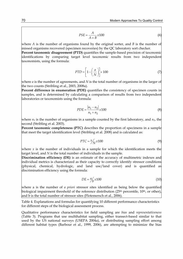
where v is the number of valid samples, and T is the total number of planned samples (Flotemersch et al., 2006). Percent sorting efficiency (PSE) describes how well a sample sorter has done in finding andremoving all specimens from isolated sample material, and is calculated as:


70

100A

PSE xA B

(6)

where A is the number of organisms found by the original sorter, and B is the number of missed organisms recovered (specimen recoveries) by the QC laboratory sort checker. Percent taxonomic disagreement (PTD) quantifies the sample-based precision of taxonomic identifications by comparing target level taxonomic results from two independenttaxonomists, using the formula:

1 100a

PTDN

(7)

where a is the number of agreements, and N is the total number of organisms in the larger ofthe two counts (Stribling et al., 2003, 2008a). Percent difference in enumeration (PDE) quantifies the consistency of specimen counts in samples, and is determined by calculating a comparison of results from two independentlaboratories or taxonomists using the formula:

1 2

1 2

100n n

PDE xn n

(8)

where n1 is the number of organisms in a sample counted by the first laboratory, and n2, the second (Stribling et al. 2003). Percent taxonomic completeness (PTC) describes the proportion of specimens in a samplethat meet the target identification level (Stribling et al. 2008) and is calculated as:

100xPTC xN (9)

where x is the number of individuals in a sample for which the identification meets thetarget level, and N is the total number of individuals in the sample. Discrimination efficiency (DE) is an estimate of the accuracy of multimetric indexes and individual metrics is characterized as their capacity to correctly identify stressor conditions(physical, chemical, hydrologic, and land use/land cover) and is quantified asdiscrimination efficiency using the formula:

100aDE xb (10)

where a is the number of a priori stressor sites identified as being below the quantifiedbiological impairment threshold of the reference distribution (25th percentile, 10th, or other), and b is the total number of stressor sites (Flotemersch et al., 2006).

Table 4. Explanations and formulas for quantifying 10 different performance characteristics for different steps of the biological assessment process.

Qualitative performance characteristics for field sampling are bias and representativeness (Table 3). Programs that use multihabitat sampling, either transect-based similar to that used by the US national surveys (USEPA 2004a), or distributing sampling effort among different habitat types (Barbour et al., 1999, 2006), are attempting to minimize the bias


71

through two components of the field method. First, the approaches are not limited to one or a few habitat types; they are focused on sampling stable undercut banks, macrophyte beds, root wads, snags, gravel, sand, and/or cobble. Second, allocation of the sampling effort is distributed throughout the entire reach, thus preventing the entire sample from being taken in a shortened portion of the reach. Further, if the predominant habitat in a sample reach is poor or degraded, that habitat would be sampled as well. These field sampling methods are intended to depict the benthic macroinvertebrate assemblage that the physical habitat in the streams and rivers has the capacity to support. Another note about representativeness is to be cognizant that, while a method might effectively depict the property it is intended to depict (Flotemersch et al., 2006), it could be interpreted differently at different spatial scales (Figure 4).

Metric RMSE Mean CV CI90

1 sample 2 samples 3 samples Number of Ephemeroptera taxa

0.94 5.25 17.9 1.55 1.1 0.89

Number of Plecoptera taxa 0.9 2.42 37.3 1.48 1.05 0.85 % individuals as EPT 8.86 47.98 18.5 14.53 10.27 8.39 % individuals as non-insects 3 7.3 41.1 4.93 3.49 2.85 % individuals as predators 5.32 16.91 31.4 8.72 6.17 5.03 % of taxa as burrowers 3.93 28.91 13.6 6.45 4.56 3.72 Hilsenhoff Biotic Index 0.47 4.27 10.9 0.76 0.54 0.44 Multimetric index (7-metric composite)

3.80 55.6 6.8 6.23 4.41 3.60

Table 5. Precision estimates for sample-based benthic macroinvertebrate metrics, and composite multimetric index (Stribling et al., 2008b). Data shown are from the US state of Montana, and performance calculations are based on 40 sample pairs from the “mountain” site class (abbreviations - RMSE, root mean square error; CV, coefficient of variation; CI90, 90 percent confidence interval; EPT, Ephemeroptera, Plecoptera, Trichoptera).

Fig, 4. Defining representativeness of a sample or datum first requires specifying the spatial and/or temporal scale of the feature it is intended to depict.


72

Accuracy is considered “not applicable” to field sampling (Table 3), because efforts to define analytical truth would necessitate a sampling effort excessive beyond any practicality. That is, the analytical truth would be all benthic macroinvertebrates that exist in the river (shore zone to 1-m depth). There is no sampling approach that will collect all individual benthic macroinvertebrate organisms.

5.2 Sorting/subsampling Bias, precision, and, in part, completeness, are quantitative characteristics of performance for laboratory sorting and subsampling (Table 3). Bias is the most critical performance characteristic of the sorting process, and is evaluated by checking for specimens that may have been overlooked or otherwise missed by the primary sorter (Flotemersch et al., 2006). Checking of the sort residue is performed by an independent sort checker in a separate laboratory using the same procedures as primary, specifically, the same magnification and lighting as called for in the SOP. The number of specimens found by the checker as a proportion of the total number of originally found specimens is the percent sorting efficiency (PSE; formula 6) (Table 4), and quantifies sorting bias. This exercise is performed on a randomly-selected subset of sort residues (generally 10% of total sample lot), the selection of which is stratified by individual sorters, by projects, or by programs. As a rule-of-thumb, an MQO could be “less than 10% of all samples checked will have a PSE ≤90%”. Table 6 shows PSE results from sort rechecks for a project within the state of Georgia (US). One sample (no. 8) exhibited a substantial failure with a PSE of 77.8, which became an immediate flag for a potential problem. Further evaluation of the results showed that the sample was fully sorted (100%), and still only 21 specimens were found by the original sorter, prior to the 6 recoveries by the re-check. Values for PSE become skewed when overall numbers are low, thus failure of this one sample did not indicate systematic error (bias) in the sorting process. Three additional samples fell slightly below the 90% MQO, but were only ≤ 0.2 percentage points low and were judged as passing by the QC analyst. Precision of laboratory sorting is calculated by use of RPD with metrics and indexes as the input variables (Table 4). If, for example, the targeted subsample size is 200 organisms, and that size subsample is drawn twice from a sorting tray without re-mixing or re-spreading, metrics can be calculated from the two separate subsamples. RPD would be an indication of how well the sample was mixed and spread in the tray; the “serial subsampling” and RPD calculations should be done on two timeframes. First, these calculations should be done, and the results documented and reported to demonstrate what the laboratory (or individual sorter) is capable of in application of the subsampling method. Second, they should be done periodically to demonstrate that the program routinely continues to meet that level of precision. Representativeness of the sorting/subsampling process is addressed as part of the SOP that requires random selection of grid squares (Flotemersch et al., 2006) with complete sorting, until the target number is reached within the final grid. Percent completeness for subsampling is calculated as the proportion of samples with the target subsample size (±20%) in the rough sort. Considered as “not applicable”, estimates of accuracy are not necessary for characterizing sorting performance.

5.3 Taxonomic precision (sample-based) Precision and completeness are quantitative performance characteristics that are used for taxonomy (Table 3). Precision of taxonomic identifications is calculated using percent taxonomic


73

Sample no. Number of specimens

PSE Original Recovered Total

1 208 5 213 97.7 2 202 8 210 96.2 3 227 1 228 99.6 4 200 12 212 94.3 5 208 7 215 96.7 6 222 2 224 99.1 7 220 24 244 90.2 8 21 6 27 77.8a

9 215 22 237 90.7 10 220 25 245 89.8b

11 220 3 223 98.7 12 211 24 235 89.8b

13 205 12 217 94.5 14 213 24 237 89.9b

15 205 11 216 94.9 16 222 15 237 93.7 17 203 10 213 95.3 18 158 16 174 90.8

a Low PSE is due to there being small total number of specimens in the

sample (n=27); this sample was also whole-pick (all 30 grid squares); b PSE values taken as passing, only ≤0.2 percentage points below MQO.

Table 6. Percent sorting efficiency (PSE) as laboratory sorting/ subsample quality control check. Results from 2006-2008 sampling for a routine monitoring program in north Georgia, USA.

disagreement (PTD) and percent difference in enumeration (PDE), both of which rely on the raw data (list of taxa and number of individuals) from whole-sample re-identifications (Stribling et al., 2003, 2008a). These two values are evaluated individually, and are used to indicate the overall quality of the taxonomic data. They can also be used to help identify the source of a problem. Percent taxonomic completeness (PTC) is calculated to document how consistently the taxonomist is able to attain the targeted taxonomic levels as specified in the SOP. It is important to note that the purpose of this evaluation approach is not to say that one taxonomist is correct over the other, but rather to make an effort to understand what is causing differences where they exist. The primary taxonomy is completed by one or more project taxonomists (T1); the re-identifications are completed as blind samples by one or more secondary, or QC taxonomists (T2) in a separate independent laboratory. The number of samples for which this analysis is performed will vary, but 10% of the total sample lot (project, program, year, or other) is an acceptable rule-of-thumb. Exceptions are that large programs (>~500 samples) may not need to do >50 samples; small programs (<~30 samples) will likely still need to do at least 3 samples. In actuality, the number of re-identified samples will be program-specific and influenced by multiple factors, such as, how


74

many taxonomists are doing the primary identification (there may be an interest in having 10% of the samples from each taxonomist re-identified), and how confident the ultimate data user is with the results. Mean values across all re-identified samples are estimates of taxonomic precision (consistency) for a dataset or a program.

5.3.1 Percent taxonomic disagreement (PTD) The sample-based error rate for taxonomic identifications is quantified by calculation of percent taxonomic disagreement (PTD) (Table 4, formula 7). The key exercise performed by the QC analyst is determining the number of matches, or shared identifications between the two taxonomists (Table 7). Matches must be exact, that is, negative comparisons result even if the difference is only hierarchical (genus vs. family, or other), whether they have been assigned different names, or whether specimens are missing from the overall results of either T1 or T2. Error typing individual sample comparisons is the process of determining differences as either: a) straight disagreements, b) hierarchical differences, or c) missing specimens. While tedious, this QC exercise provides information that is extremely valuable in formulating corrective actions. An MQO of 15% has been found to be attainable by most programs, and is used for the USEPA national surveys. As testing continues and laboratories and taxonomists become more accustomed to the procedure, it is becoming apparent that potentially the national standard could eventually be set at 10%. A standard summary report for taxonomic identification QC (Table 8) can be effectively communicated to data users.

5.3.2 Percent difference in enumeration (PDE) Another summary data quality indicator for performance in taxonomic identification is comparison of the total number of organisms counted and reported in the sample by the two taxonomists (not the sorters). There is some redundancy of this measure with PTD, but it has proven useful in helping highlight coarse differences immediately, and is calculated as percent difference in enumeration (PDE) (Table 4, formula 8). While sorters may be well-trained, experienced, and have substantial internal QC oversight, they may not always be able to determine identifiability, the final decision of which is the responsibility of the taxonomist. It is rare to find exact agreement on sample counts between two taxonomists but the differences are usually minimal, hence the low recommended MQO of 5%. When PDE>5, reasons are usually fairly obvious, and the QC analyst can turn attention directly to the error source to determine if it may be systematic, and the nature and necessity of corrective action(s).

5.3.3 Percent taxonomic completeness (PTC) Percent taxonomic completeness (PTC) (Table 3, formula 9) quantifies the proportion of individuals in a sample that are identified to the specified target taxonomic level (Table 1). Results can be interpreted in a number of ways: the individuals in a sample are damaged or early instar, many are damaged with diagnostic characters missing (such as, gills, legs, antennae, etc.) or the taxonomist is inexperienced or unfamiliar with the particular taxon. MQO have not been used for this characteristic, but barring an excessively damaged sample, it is not uncommon to see PTC in excess of 97 or 98. For purposes of QC, it is more important to have the absolute difference (abs diff) of PTC between T1 and T2 to be a low number, as documentation of consistency of effort; those values are often typical at 5-6%, or below.


75

Sample no.

Count No.

matches PDE PTD

Target level (taxonomic completeness)

T1 T2 T1 PTC T2 PTC Abs diff

1 243 244 232 0.2 4.9 234 96.3 223 91.4 4.9 2 227 223 204 0.9 10.1 205 90.3 194 87.0 3.3 3 214 213 191 0.2 10.7 202 94.4 199 93.4 1.0 4 221 223 207 0.5 7.2 212 95.9 208 93.3 2.6 5 216 214 202 0.5 6.5 207 95.8 201 93.9 1.9 6 216 216 214 0 0.9 209 96.8 208 96.3 0.5 7 86 83 69 1.8 19.8 77 89.5 64 77.1 12.4 8 206 201 194 1.2 5.8 204 99 187 93.0 6.0 9 208 210 196 0.5 6.7 203 97.6 195 92.9 4.7

10 192 195 180 0.8 7.7 182 94.8 172 88.2 6.6

Table 7. Summary table for sample by sample taxonomic comparison results, from routine biological monitoring in US state of Mississippi. T1 and T2 are the primary and QC taxonomists, respectively. “No. matches” is the number of individual specimens counted and given the same identity by each taxonomist, and PDE, PTD, and PTC are explained in text. Target level is the number and percentage of specimens identified to the SOP-specified level of effort (see Table 3 as an example); “Abs diff” is the absolute difference between the PTC of T1 and T2.

A. Number of samples in lot 97 B. Number of samples used for taxonomic comparison 10 C. Percent of sample lot 10.3% D. Percent taxonomic disagreement (PTD) 1. MQO 15 2. No. samples exceeding 1 3. Average 7.9 4. Standard deviation 4.9 E. Percent difference in enumeration (PDE) 1. MQO 5 2. No. samples exceeding 0 3. Average 0.6 4. Standard deviation 0.6 F. Percent taxonomic completeness (PTC, absolute difference) 1. MQO none 2. Average 4.3 3. Standard deviation 3.5

Table 8. Taxonomic comparison results from a bioassessment project in the US state of Mississippi.

5.4 Taxonomic accuracy (taxon-based) Accuracy and bias (the inverse of accuracy) are quantitative performance characteristics for taxonomy (Table 3). Accuracy requires specification of an analytical truth, and for taxonomy


76

that is 1) the museum-based type specimen (holotype, or other form of type specimen), 2) specimen(s) verified by recognized expert(s) in that particular taxon or 3) unique morphological characteristics specified in dichotomous identification keys. Determination of accuracy is considered “not applicable” for production taxonomy (most often used in routine monitoring programs) because that kind of taxonomy is focused on characterizing the sample; taxonomic accuracy, by definition, would be focused on individual specimens. Bias in taxonomy can result from use of obsolete nomenclature and keys, imperfect understanding of morphological characteristics, inadequate optical equipment, or poor training. Neither of these performance characteristics is considered necessary for production taxonomy, in that they are largely covered by the estimates of precision and completeness. For example, although it is possible that two taxonomists would put an incorrect name on an organism, it is considered low probability that they would put the same incorrect name on that organism.

5.5 Data entry accuracy Recognition and correction of data entry errors (even the one mentioned in Section 4.3) could come from one of two methods for assuring accuracy in data entry; both do not need to be done. One is the double entry of all data by two separate individuals, and then performing a direct match between databases. Where there are differences, it is determined which database is in error, and corrections are made. The second approach is to perform a 100% comparison of all data entered to handwritten data sheets. Comparisons should be performed by someone other than the primary data entry person. When errors are found, they are hand-edited for documentation, and corrections are made electronically. The rates of data entry errors are recorded and segregated by data type (e.g., fish, benthic macroinvertebrates, periphyton, header information, latitude and longitude, physical habitat, and water chemistry). Issues could potentially arise when entering data directly into field e-tablets or laboratory computers. Because there would be no paper backup, QC checks of data entry are not possible.

5.6 Site assessment and interpretation Quantitative performance characteristics for site assessment and interpretation are precision, accuracy, and completeness (Table 3). Site assessment precision is based on the narrative assessments from the associated index scores (good, fair, poor) from reach duplicates and quantifies the percentage of duplicate samples that are receiving the same narrative assessments. These comparisons are done for a randomly-selected 10% of the total sample lot. Table 9 shows this direct comparison that, for this dataset, 79% of the replicates returned assessments of the same category (23 out of 29); 17% were 1 category different (5 of 29); and 3% were 2 categories different (1 of 29). Assessment accuracy is expressed using discrimination efficiency (DE) (formula 10; Table 4), a value developed during the index calibration process, which relies upon, first, specifying magnitudes of physical, chemical, and/or hydrologic stressors that are unacceptable, and identifying those sites exhibiting those excessive stressor characteristics. The set of sites exhibiting unacceptable stressor levels constitute the analytical truth. The proportion of samples for which the biological index correctly identifies sites as impaired is DE. This is a performance characteristic that is directly suitable for expressing how well an indicator does what it is designed to do, detect stressor conditions, but it is not suitable for routine QC analyses. Percent completeness (%C) is the proportion of sites (of the total planned) for which valid final assessments were obtained.


77

6. Maintenance of data quality

The purpose of QC is to identify assignable causes of variation (error) so that the quality of the outcomes in future processes can be made, on average, less variable (Shewhart, 1939). For reducing error rates, it is first and foremost critical to know of the existence of error, and second, to know its causes. Once the causes are known, corrective actions can be designed to reduce or eliminate them. The procedures described in this chapter for gathering information that allow performance and data quality characteristics to be documented need to become a routine part of biological monitoring programs. If they are used only when “conditions are right”, as part of special studies, or when there are additional resources, they are not serving their purpose and could ultimately be counter-productive. The counter-productivity would arise when monitoring staff begin to view QC samples and analyses as activities that are less than routine, and something for which to strive to do their best, that is, only when they are being tested. This perspective leads programs to work to meet a number, such as 15%, rather than using the information to maintain or improve.

Site Replicate 1 Replicate 2

Categorical difference Narrative Assessment

category Narrative Assessment category

A Poor 3 Poor 3 0 B Poor 3 Poor 3 0 C Good 1 Good 1 0 D Poor 3 Very Poor 4 1 E Fair 2 Fair 2 0 F Poor 3 Fair 2 1 G Poor 3 Poor 3 0 H Very Poor 4 Very Poor 4 0 I Very Poor 4 Very Poor 4 0 J Poor 3 Poor 3 0 K Poor 3 Poor 3 0 L Very Poor 4 Very Poor 4 0 M Very Poor 4 Very Poor 4 0 N Poor 3 Fair 2 1 O Poor 3 Poor 3 0 P Poor 3 Poor 3 0 Q Poor 3 Very Poor 4 1 R Poor 3 Poor 3 0 S Fair 2 Very Poor 4 2 T Fair 2 Fair 2 0 U Good 1 Good 1 0 V Poor 3 Fair 2 1 W Fair 2 Fair 2 0 X Poor 3 Poor 3 0 Y Poor 3 Poor 3 0 Z Very Poor 4 Very Poor 4 0

AA Poor 3 Poor 3 0 BB Fair 2 Fair 2 0 CC Poor 1 Poor 1 0

Table 9. Assessment results shown for sample pairs taken from 29 sites, each pair representing two adjacent reaches (back to back (see Fig. 4). Assessment categories are 1 – good, 2 – fair, 3 – poor, and 4 – very poor.


78

Performance characteristic MQO

Field sampling precision (multimetric index)

CV < 10%, for a sampling event (field season, watershed, or other strata)


CI90 ≤ 15 index points, on a 100-point scale


RPD < 15

Field sampling completeness Completeness > 98%

Sorting/subsampling accuracy PSE≥90, for ≥ 90% of externally QC’d sort residues

Taxonomic precision Median PTD ≤ 15% for overall sample lot; samples with PTD ≥ 15% examined for patterns of error

Taxonomic precision Median PDE ≤ 5%; samples with PDE ≥ 5% should be further examined for patterns of error

Taxonomic completeness Median PTC ≥ 90%; samples with PTC ≤ 90% should be examined and those taxa not meeting targets isolated; mAbs diff ≤ 5%

Table 10. Key measurement quality objectives (MQO) that could be used to track maintenance of data quality at acceptable levels.

Key to maintaining data quality of known and acceptable levels is establishing performance standards based on MQO. Qualitative standards, such some of the representativeness and accuracy factors (Table 3), can be evaluated by comparing SOP and SOP application to the goals and objectives of the monitoring program. However, a clear statement of data quality expectations, such as that shown in Table 10, will help to ensure consistency of success in implementing the procedures. As a program becomes more proficient and consistent in meeting the standards, efforts could be undertaken to “tighten up” the standards. With this comes necessary budgetary considerations; better precision can always be attained, but often at elevated costs.

7. Comparability analysis and acceptable data quality

All discussion to this point has been directed toward documenting data quality associated with monitoring programs, hopefully with sufficient emphasis that there are no data that are right or wrong, but just that they are acceptable or not. If data are acceptable for a decision (for example, in the context of biological assessment and monitoring), a defensible statement on the ecological condition of a site or an ecological system can be made. If they are not acceptable to support that decision, likewise, the decision not to use the data should also be defensible. Routine documentation and reporting of data quality within a monitoring program provides a statement of intra-programmatic consistency, that is, sample to sample comparability even if collected from different temporal or spatial scales. If there is an interest in or need to combine datasets from different programs (Figure 5), it is imperative for routinely documented performance characteristics be available for each. Lack of them will preclude any determination of acceptability for decision making by data users, whether scientists, policy-makers, or the public.


79

Fig. 5. Framework for analysis of comparability between or among monitoring datasets or protocols.

8. Conclusion

If data of unknown quality are used, whether by themselves or in combination with others, the assumption is implicit that they are acceptable, and hence, comparable. We must acknowledge the risk of incorrect decisions when using such data and be willing to communicate those risks to both data users and other decisionmakers. The primary message of this chapter is that appropriate and sufficient QC activities should be a routine component of any monitoring program, whether it is terrestrial or aquatic, focuses on physical, chemical, and/or biological indicators, and, if biological, whether it includes macroinvertebrates, algae/diatoms, fish, broad-leaf plants, or other organism groups.

9. References

APHA. 2005. Standard Methods for the Examination of Water and Wastewater. 21st edition. American Public Health Association, American Water Works Association, and Water Environment Federation, Washington, DC.

Barbour, M.T., & J. Gerritsen. 1996. Subsampling of benthic samples: a defense of the fixed count method. Journal of the North American Benthological Society 15:386- 391.

Dataset or protocol A(performance characteristics)

Dataset or protocol B(performance characteristics)

Compare Apc to Bpc

Acceptable data quality?

YES NOCombine into single dataset;

proceed with analysesExclude from analyses, or adjust

with corrective approaches


80

Barbour, M.T., J. Gerritsen, B.D. Snyder, J.B. Stribling. 1999. Rapid Bioassessment Protocols for Streams and Wadeable Rivers: Periphyton, Benthic Macroinvertebrates and Fish. Second edition. EPA/841-D-97-002. U.S. EPA, Office of Water, Washington, DC. URL:

http://water.epa.gov/scitech/monitoring/rsl/bioassessment/index.cfm. Barbour, M. T., J. B. Stribling, & P.F.M. Verdonschot. 2006. The multihabitat approach of

USEPA’s rapid bioassessment protocols: Benthic macroinvertebrates. Limnetica 25(3-4): 229-240.

Blocksom, K.A., & J.E. Flotemersch. 2005. Comparison of macroinvertebrate sampling methods for non-wadeable streams. Environmental Monitoring and Assessment 102:243-262.

Blocksom, K.A., & J.E. Flotemersch. 2008. Field and laboratory performance characteristics of a new protocol for sampling riverine macroinvertebrate assemblages. River Research and Applications 24: 373–387. DOI: 10.1002/rra.1073

Bortolus, A. 2008. Error cascades in the biological sciences: the unwanted consequences of using bad taxonomy in ecology. Ambio 37(2): 114-118.

Brunialti, G., P. Giordani, & M. Ferretti. 2004. Discriminating between the Good and the Bad: Quality Assurance Is Central in Biomonitoring Studies. Chapter 20, pp. 443-464, IN, G.B. Wiersma (editor), Environmental Monitoring. CRC Press.

Cao, Y., & C.P. Hawkins. 2005. Simulating biological impairment to evaluate the accuracy of ecological indicators. Journal of Applied Ecology 42:954-965.

Cao, Y., C.P. Hawkins, & M.R. Vinson. 2003. Measuring and controlling data quality in biological assemblage surveys with special reference to stream benthic macroinvertebrates. Freshwater Biology 48: 1898–1911.

Carter, J.L. & V.H. Resh. 2001. After site selection and before data analysis: sampling, sorting, and laboratory procedures used in stream benthic macroinvertebrate monitoring programs by USA state agencies. Journal of the North American Benthological Society 20: 658-676.

Caton, L. R. 1991. Improved subsampling methods for the EPA rapid bioassessment benthic protocols. Bulletin of the North American Benthological Society 8:317-319.

Clarke, R.T., M.T. Furse, J.F. Wright & D. Moss. 1996. Derivation of a biological quality index for river sites: comparison of the observed with the expected fauna. Journal of Applied Statistics 23:311–332.

Clarke, R.T., J.F. Wright & M.T. Furse. 2003. RIVPACS models for predicting the expected macroinvertebrate fauna and assessing the ecological quality of rivers. Ecological Modeling 160:219–233.

Costanza, R., S.O. Funtowicz & J.R. Ravetz. 1992. Assessing and communicating data quality in policy-relevant research. Environmental Management 16(1):121- 131.

Courtemanch, D.L. 1996. Commentary on the subsampling procedures used for rapid bioassessments. Journal of the North American Benthological Society 15:381- 385.

Deming, W.E. 1986. Foreward. In, Shewhart, W.A. 1939. Statistical Methods from the Viewpoint of Quality Control. The Graduate School, U.S. Department of Agriculture,


81

Washington, DC. 105 pp. Republished 1986, with a new Foreword by W.E. Deming. Dover Publications, Inc., 31 East 2nd Street, Mineola, NY.

Diamond, J.M., M.T. Barbour & J.B. Stribling. 1996. Characterizing and comparing bioassessment methods and their results: a perspective. Journal of the North American Benthological Society 15:713-727.

Edwards, P.N. 2004. “A vast-machine”: Standards as social technology. Science 304 (7):827-828.

Flotemersch, J.E. & K.A. Blocksom. 2005 Electrofishing in boatable rivers: Does sampling design affect bioassessment metrics? Environmental Monitoring and Assessment 102:263-283. DOI: 10.1007/s10661-005-6026-2

Flotemersch J.E., J.B. Stribling, & M.J. Paul. 2006. Concepts and Approaches for the Bioassessment of Non-Wadeable Streams and Rivers. EPA/600/R-06/127. U.S. Environmental Protection Agency, Cincinnati, OH.

Flotemersch, J.E., J.B. Stribling, R.M. Hughes, L. Reynolds, M.J. Paul & C. Wolter. 2010. Site length for biological assessment of boatable rivers. River Research and Applications. Published online in Wiley InterScience

(www.interscience.wiley.com) DOI: 10.1002/rra.1367. General Accounting Office (GAO). 2004. Watershed Management: Better Coordination of Data

Collection Efforts. GAO-04-382. Washington, DC , USA. Available from: <http://www.gao.gov/new.items/d04382.pdf>.

Gurtz, M.E. & T.A. Muir (editors). 1994. Report of the Interagency Biological Methods Workshop. U.S. Geological Survey, Open File Report 94-490, Reston, Virginia, USA.

Haase, P., J. Murray-Bligh, S. Lohse, S. Pauls, A. Sundermann, R. Gunn & R. Clarke. 2006. Assessing the impact of errors in sorting and identifying macroinvertebrate samples. Hydrobiologia 566:505–521. DOI 10.1007/s10750-006-0075-6

Hawkins, C.P. 2006. Quantifying biological integrity by taxonomic completeness: evaluation of a potential indicator for use in regional- and global-scale assessments. Ecological Applications 16:1277–1294.

Hawkins, C.P., R.H. Norris, J.N. Hogue & J.W. Feminella. 2000. Development and evaluation of predictive models for measuring the biological integrity of streams. Ecological Applications 10:1456–1477.

Heinz Center, The. 2002. The state of the nation’s ecosystems: measuring the lands, waters, and living resources of the United States. The H. John Heinz III Center for Science, Economics, and the Environment, Washington, DC, USA. Cambridge University Press. Available from:

<http://www.heinzctr.org/ecosystems/index.htm>. Herbst, D.B. & E.L. Silldorf. 2006. Comparison of the performance of different bioassessment

methods: similar evaluations of biotic integrity from separate programs and procedures. Journal of the North American Benthological Society 25:513–530.

Hill, B.H., A.T. Herlihy, P.R. Kaufmann, S.J. Decelles & M.A. Vander Borgh. 2003. Assessment of streams of the eastern United States using a periphyton index of biotic integrity. Ecological Indicators 2:325–338.


82

Hill, B.H., A.T. Herlihy, P.R. Kaufmann, R.J. Stevenson, F.H. McCormick & C.B. Johnson. 2000. Use of periphyton assemblage data as an index of biotic integrity. Journal of the North American Benthological Society 19:50–67.

Hughes, R.M., P.R. Kaufmann, A.T. Herlihy, T.M. Kincaid, L. Reynolds & D.P. Larsen. 1998. A process for developing and evaluating indices of fish assemblage integrity. Canadian Journal of Fisheries and Aquatic Sciences 55:1618–1631.

ITFM. 1995a. The Strategy for Improving Water Quality Monitoring in the U.S. Intergovernmental Task Force on Monitoring Water Quality. Report #OFR95-742, U.S. Geological Survey, Reston, Virginia, USA.

ITFM. 1995b. Performance-based approach to water quality monitoring. In: Strategy for Improving Water Quality Monitoring in the U.S., Appendix M, Report #OFR95-742, Intergovernmental Task Force on Monitoring Water Quality, U.S. Geological Survey, Reston, Virginia, USA.

Karr, J.R., K.D. Fausch, P.L. Angermeier, P.R. Yant & I.J. Schlosser. 1986. Assessing Biological Integrity in Running Waters: a Method and its Rationale. Special publication 5. Illinois Natural History Survey, Champaign, Illinois, USA.

Keith, L.H. (editor). 1988. Principles of Environmental Sampling. ACS Professional Reference Book. American Chemical Society, Columbus, Ohio.

Keith, L.H. 1991. Environmental Sampling and Analysis. A Practical Guide. Lewis Publishers, Chelsea, Michigan.

Klemm, D.J., P.A. Lewis, F. Fulk & J.M. Lazorchak. 1990. Macroinvertebrate Field and Laboratory Methods for Evaluating the Biological Integrity of Surface Waters. EPA/600/4-90/030. Environmental Monitoring Systems Laboratory, U.S. Environmental Protection Agency, Cincinnati, OH. 256 pp.

Klemm, D.J., J.M. Lazorchak & P.A. Lewis. 1998. Benthic macroinvertebrates. Pages 147–182 in J. M. Lazorchak, D. J. Klemm, and D. V. Peck (editors). Environmental Monitoring and Assessment Program—Surface Waters: Field Operations and Methods for Measuring the Ecological Condition of Wadeable Streams. EPA/620/R-94/ 004F. U.S. Environmental Protection Agency, Washington, DC.

Lindley, D. 2007. Uncertainty. Einstein, Heisenberg, Bohr, and the Struggle for the Soul of Science. Anchor Books, a Division of Random House. ISBN: 978-1-4000-7996-4. New York, NY. 257 pp.

Merritt, R.W., K.W. Cummins & M.B. Berg (editors). 2008. An Introduction to the Aquatic Insects of North America. Fourth Edition. Kendall/Hunt Publishing Company, Dubuque, Iowa. ISBN 978-0-7575-5049-2. 1158 pp.

Milberg, P., J. Bergstedt, J. Fridman, G. Odell & L. Westerberg. 2008. Systematic and random variation in vegetation monitoring data. Journal of Vegetation Science 19: 633-644. http://dx.doi.org/10.3170/2008-8-18423.

Montana DEQ. 2006. Sample collection, sorting, and taxonomic identification of benthic macroinvertebrates. Standard operation procedure. WQPBWQM-009. Revision no. 2. Water Quality Planning Bureau, Montana Department of Environmental Quality, Helena, Montana. (Available from:

http://www.deq.mt.gov/wqinfo/QAProgram/ WQPBWQM-009rev2_final_web. pdf)


83

NWQMC. 2001. Towards a Definition of Performance-Based Laboratory Methods. National Water Quality Monitoring Council Technical Report 01 – 02, U.S. Geological Survey, Reston, Virginia, USA.

Nichols, S.J., W.A. Robinson & R.H. Norris. 2006. Sample variability influences on the precision of predictive bioassessment. Hydrobiologia 572: 215–233. doi 10.1007/s10750-005-9003-4

Peters, J.A. 1988. Quality control infusion into stationary source sampling. Pages 317–333 in L. H. Keith (editor). Principles of Environmental Sampling. ACS Professional Reference Book. American Chemical Society, Columbus, Ohio.

Shewhart, W.A. 1939. Statistical Methods from the Viewpoint of Quality Control. The Graduate School, U.S. Department of Agriculture, Washington, DC. 105 pp. Republished 1986, with a new Foreword by W.E. Deming. Dover Publications, Inc., 31 East 2nd Street, Mineola, NY.

Smith, R.-K. 2000. Interpretation of Organic Data. ISBN 1-890911-19-4. Genium Publishing Corporation. Genium Group, Inc., Amsterdam, New York.

Stribling, J. B., S.R. Moulton II & G.T. Lester. 2003. Determining the quality of taxonomic data. Journal of the North American Benthological Society 22(4): 621-631.

Stribling, J.B., K.L. Pavlik, S.M. Holdsworth & E.W. Leppo. 2008a. Data quality, performance, and uncertainty in taxonomic identification for biological assessments. Journal of the North American Benthological Society 27(4): 906-919. doi: 10.1899/07-175.1

Stribling, J.B., B.K. Jessup & D.L. Feldman. 2008b. Precision of benthic macroinvertebrate indicators of stream condition in Montana. Journal of the North American Benthological Society 27(1):58-67. doi: 10.1899/07-037R.1

Taylor, J.K. 1988. Defining the Accuracy, Precision, and Confidence Limits of Sample Data. Chapter 6, pages 102-107, IN Lawrence H. Keith (editor), Principles of Environmental Sampling. ACS Professional Reference Book. ISBN 0-8412-1173-6. American Chemical Society. Columbus, Ohio.

Taylor, J.R. 1997. An Introduction to Error Analysis. The Study of Uncertainties in Physical Measurements. Second edition. University Science Books, Sausalito, California, USA.

Taylor, B.N. & C.E. Kuyatt. 1994. Guidelines for Evaluating and Expressing the Uncertainty of NIST Measurement Results. NIST Technical Note 1297. National Institute of Standards and Technology, U.S. Department of Commerce, Washington, DC. 24 pp.

USEPA. 2004a. Wadeable Stream Assessment: Field Operations Manual. EPA 841-B-04-004. Office of Water and Office of Research and Development, US Environmental Protection Agency, Washington, DC.

USEPA. 2004b. Wadeable Stream Assessment: Benthic Laboratory Methods. EPA 841-B-04007. Office of Water and Office of Research and Development, US Environmental Protection Agency, Washington, DC.

U. S. GPO (Government Printing Office). 1989. Federal Water Pollution Control Act (33 U. S. C. 1251 et seq.) as amended by a P. L. 92-500. In: Compilation of selected water


84

resources and water pollution control laws. Printed for use of the Committee on Public Works and Transportation. Washington, DC, USA.

Vinson, M.R. & C.P. Hawkins. 1996. Effects of sampling area and subsampling procedure on comparisons of taxa richness among streams. Journal of the North American Benthological Society 15:392-399.

Zar, J.H. 1999. Biostatistical Analysis. 4th edition. Prentice Hall, Upper Saddle River, New Jersey, USA.

Proper citation: Stribling, James B. 2011. Partitioning Error Sources for Quality Control and Comparability Analysisin Biological Monitoring and Assessment. Chapter 4 (pp. 59-84), IN, Eldin, A.B. (editor), Modern Approaches to Quality Control. ISBN 978-953-307-971-4. InTech Open Access Publisher. DOI: 10.5772/22388. http://www.intechopen.com/articles/show/title/partitioning-error-sources-for-quality-control-and-comparability-analysis-in-biological-monitoring-a

http://www.intechopen.com/articles/show/title/partitioning-error-sources-for-quality-control-and-comparability-analysis-in-biological-monitoring-a

biological monitoring quality control - advisory committee on water

Documents