3 biological monitoring of aquatic communities
TRANSCRIPT

3 BIOLOGICAL MONITORING OF AQUATIC COMMUNITIES
3.1 INTRODUCTION
Biological monitoring, as described here, consists of assessing the condition of the physical habitat and specific biological assemblages—typically benthic macroinvertebrates and fish— that inhabit the aquatic environment. In the true definition of the term, biological monitoring includes toxicity testing, fish tissue analyses, and single population surveys conducted over time. However, for purposes of this document, the definition of biological monitoring is limited to the concept of community-level assessments.
Community: Any group of organisms of different species that co-occur in the same habitat or area.
This chapter discusses the rationale behind using biological monitoring as part of a nonpoint source (NPS) monitoring program, gives basic guidance on conducting biological assessments, provides biological monitoring program design considerations, and discusses ways in which biological assessment data can be used to detect trends in NPS impacts. Numerous texts and papers have been written on biological monitoring methods (see references), but methods and means of interpreting the results from them are still under development for many habitats and regions of the country. The U.S. Environmental Protection Agency (EPA) has produced two guidance documents that are the foundation for the majority of state biological monitoring programs:
• Biological criteria: Technical guidance for streams and small rivers. EPA 822-B-96-001. (Gibson et al., 1996)
• Rapid bioassessment protocols for use in streams and wadable rivers. EPA/444/4-89001. (Plafkin et al., 1989)
Many state agencies, such as the Ohio Environmental Protection Agency (OEPA), Illinois Environmental Protection Agency (IEPA), Delaware Department of Natural Resource and Environmental Control (DNREC), Florida Department of Environmental Protection (DEP), Connecticut DEP, and New York Department of Environmental Conservation (DEC), are incorporating biological monitoring into ongoing and new monitoring programs. In addition, numerous ongoing biological monitoring programs have been implemented by federal, local, and tribal entities, including the U.S. Geological Survey (USGS), National Water Quality Assessment Program (NAWQA); U.S. Department of the Interior, Bureau of Land Management; U.S. Department of Agriculture (USDA), Forest Service; King County, Washington; Prince George’s County, Maryland; and the Yakama Tribe. The methods for biological monitoring are thereby being improved, and this in turn is making biological assessment a more widely accepted and applicable tool for monitoring programs.
The common use of EPA methods for sampling and analysis is documented in a recent work that reviews state programs (Summary of state biological assessment programs for streams and wadable rivers, Davis et al., 1996; EPA230-R-96007). It shows that 45 states are using rapid bioassessment protocol (RBP)-type sampling and analysis methods or are in the process of establishing such programs.
Biological survey approaches differ depending on the waterbody, i.e., stream, river, lake, estuary, or wetland. EPA has developed and or is currently developing bioassessment survey methods appropriate for use in these different waterbody types.
3-1
Biological Monitoring Chapter 3
3.1.1 Rationale and Strengths of Biological Assessment
The central purpose of assessing biological condition is to determine how well a waterbody supports aquatic life and what kind of aquatic life it supports. Biological communities reflect the cumulative effects of different pollutant stressors—excess nutrients, toxic chemicals, increased temperature, excessive sediment loading, and others—and thus provide an overall measure of the aggregate impact of the stressors. Although biological communities respond to changes in water quality more slowly than water quality actually changes, they respond to stresses of various degrees over time. Because of this, monitoring changes in biological communities can be particularly useful for determining the impacts of infrequent or low-level stresses, such as highly variable NPS pollutant inputs, which are not always detected with episodic water chemistry measurements. Improvements in waterbody condition after the implementation of best management practices (BMPs) can sometimes be difficult to detect, and biological assessment can be useful for measuring such improvements. Several biosurvey techniques that can be used for detecting aquatic life impairments and assessing their relative severity are discussed in this chapter.
A small number of factors are often key in determining the structure of a community and its response to stress; e.g., the type of substrate or the riparian vegetation that provides organic material to the stream, regulates temperature, and provides bank stability (National Research Council, 1986). Landscape features such as soil type, vegetation, surrounding land use, and climate also have a well-documented influence on water chemistry and hydrologic characteristics. Finally, water quality, as influenced by landscape features and anthropogenic sources of pollutants, has a direct effect on aquatic biological communities.
The quality of the physical habitat is an important factor in determining the structure of benthic macroinvertebrate, fish, and periphyton assemblages. The physical features of a habitat include substrate type, amount of debris in the waterbody, amount of sunlight entering the habitat, water flow regime (in streams and rivers), and type and extent of aquatic and riparian vegetation. Even though there might not be sharp boundaries between habitat features in a stream, such as riffles and pools, the biota inhabiting them are often taxonomically and biologically distinct (Hawkins et al., 1993). Habitat quality is assessed during biological assessment and is a measure of the extent to which the habitat provides a suitable environment for healthy biological communities.
Biological assessment: An evaluation of the biological condition of a waterbody using biological surveys and other direct measurements of biota in surface waters.
Biological monitoring: Multiple, routine biological assessments over time using consistent sampling and analysis methods for the detection of changes in biological condition.
Natural biological communities are usually diverse, comprising species at various trophic levels (e.g., primary producers, secondary producers, carnivores) and levels of sensitivity to environmental changes. Adverse impacts from NPS pollution or other stressors such as habitat alteration can reduce the number of species in a community, change the relative abundances of species within a community, or alter the trophic structure of a community. Biological surveys of select species or types of organisms that are particularly sensitive to stressors, such as fish, periphyton, or benthic macroinvertebrates, take
3-2

Chapter 3 Biological Monitoring
advantage of this sensitivity as a means to evaluate the collective influence of the stressors on the biota (Cummins, 1994).
Some NPS pollutant inputs such as wet-weather runoff of chemical contaminants or sediment are highly variable in time, and biological monitoring can be a useful approach for monitoring this type of NPS impact. Biological monitoring can be used to assess the overall impact of multiple stressors, although it might not provide information about the relative magnitude of each stressor.
Knowledge of the natural physical habitat and biological communities in an area is important for interpreting biological assessment data. Biological and habitat data collected from numerous sites that are in good or near-natural condition can be used to determine the type of biological community that should be found in a particular aquatic habitat. In areas where natural conditions do not exist (due to past disturbances), historical data or the best professional judgment of knowledgeable experts can sometimes be used to select reference sites and define the reference condition. This natural condition has been referred to as reflecting biological integrity, defined by Karr and Dudley (1981) as “the capability of supporting and maintaining a balanced, integrated, adaptive community of organisms having a species composition, diversity, and functional organization comparable to that of the natural habitat of the region.” Highly detailed biological assessments are comparisons of biological conditions at a test site to the expected natural community and are thus a measure of the degree to which a site supports (or does not support) its “ideal” or potential biological community (Gibson et al., 1996). Other types of biological assessment involve comparisons of impacted sites to control sites, the latter being sites that are similar to monitored sites but are not
affected by the stresses that affect the monitored sites (Skalski and McKenzie, 1982). Paired watersheds or upstream-downstream approaches are examples. A knowledge of the natural condition is still valuable for accurate data interpretation when control sites are used (Cowie et al., 1991).
3.1.2 Limitations of Biological Assessment
Although biological assessment is useful for detecting impairments to aquatic life and assessing the severity of the impairments, it is not necessarily a measure of specific stressors. Thus, it usually does not provide information about the cause of impairment, i.e., specific pollutants or their sources. Certain biological indicators do provide information about the types of stress affecting a biological community. However, if stress to a stream community is chemical, chemical monitoring in addition to biological monitoring is required to determine the actual pollutants responsible for biological or water quality impairments and their sources. Chemical monitoring and toxicity tests are also necessary to design appropriate pollution control programs.
Biological integrity: “The capability of supporting and maintaining a balanced, integrated, adaptive community of organisms having a species composition, diversity, and functional organization comparable to that of the natural habitat of the region” (Karr and Dudley, 1981).
3-3

Biological Monitoring Chapter 3
A detailed biological monitoring program requires the development of the analysis protocols for biological assessments (including reference conditions and metrics, which are discussed later). Establishing the analysis approach can require a considerable level of effort and therefore can be somewhat expensive. Also, detailed biological assessments generally require precise training and broad experience with taxonomic identification of the samples. Experience in the region where sampling is to occur is helpful, but not required. The biological assessment methods and the means of interpreting the results from assessments need to be tailored to many habitats and regions of the country. Establishing a biological assessment and monitoring program can require a significant investment of time, staff, and money. However, the majority of these are one-time, up-front investments dedicated to the establishment of reference conditions, standard operating procedures, and a programmatic quality assurance and quality control plan.
Finally, there can often be a lag between the time at which a toxic contaminant or some other stressor is introduced into a waterbody and a detectable biological response. Consequently, biological monitoring is not appropriate for determining system response due to short-term stresses, such as storms. Similarly, there is often a lag time in the improvement of biological communities following habitat restoration or pollution problem abatement. The extent of this lag time is difficult, if not impossible, to predict. Other factors also determine the rate at which a biological community recovers, e.g., the availability of nearby populations of species for recolonization following pollution mitigation and the extent or magnitude of ecological damage done during the period of perturbation (Richards and Minshall, 1992). In extreme cases, a biological community might not recover following pollution abatement or
habitat restoration. Both the possibility of the failure of a biological community to recover from perturbation and unpredictable lag times before improvement is noticeable have obvious implications for the applicability of biological monitoring to some NPS pollution monitoring objectives. Table 3-1 summarizes the strengths and limitations of the biomonitoring approach.
3.2 HABITAT ASSESSMENT
Habitat assessment is an important component of biological assessment and monitoring, both in describing the biological potential of a system and in addressing the Clean Water Act emphasis on “physical integrity.” As mentioned in the introduction, the quality of the physical habitat is important in determining the structure of benthic macroinvertebrate and fish communities. Habitat quality refers to the extent to which habitat structure provides a suitable environment for healthy biological communities to exist. Habitat quality encompasses the three factors habitat structure, flow regime, and energy source. Habitat structure refers to the physical characteristics of stream environments. It comprises channel morphology (width, depth, sinuosity); floodplain shape and size; channel gradient; instream cover (boulders, woody debris); substrate types and diversity; riparian vegetation and canopy cover; and bank stability. Flow regime is defined by the velocity and volume of water moving through a stream. Energy enters streams as the input of nutrients in runoff or ground water, as debris (e.g., leaves) falling into streams, or from photosynthesis by aquatic plants and algae.
These three factors—habitat structure, flow regime, and energy source—are interrelated and make stream environments naturally heterogeneous. Habitat structural features that
3-4

Chapter 3 Biological Monitoring
Table 3-1. General strengths and limitations of biological monitoring and assessment approaches.
Strengths Limitations
Properly developed methods, metrics, and reference conditions provide a tool that provides a means to assess the ecological condition of a waterbody
Simpler bioassessments can be relatively inexpensive and easily performed with minimal training
Bioassessment indicates the cumulative impacts of multiple stressors on biological communities, not only water quality
Biological assessment data can be interpreted based on regional reference conditions where reference sites for the immediate area being monitored are not available
Bioassessments involving 2 or more organism groups at different trophic levels provide a reasonable assessment of ecosystem health
Biological community condition reflects both short- and long-term effects
Development of regional methods, metrics, and reference conditions takes considerable effort and an organized and well-thought-out design
Rigorous bioassessment can be expensive and requires a higher level of training and expertise to implement
Basic biological assessment information does not provide information on specific cause-effect relationships
There may be a lag time between pollution abatement or BMP installation and community recovery, so monitoring over time is required for trend detection
The optimal season for biological sampling season varies regionally, and sampling during multiple seasons may be required in some areas
Biological assessment does not always distinguish between the effects of different stressors in a system impacted by more than one stressor
determine the assemblages of macroinvertebrates can differ greatly within small areas—or microhabitats—or in short stretches of a stream. For instance, woody debris in a stream affects the flow in the immediate area, provides a source of energy, and offers protection to aquatic organisms. Curvature (sinuosity) in a stream affects currents and thereby deposition of sediment on the inner and outer banks. Rocks and boulders create turbulence, which affects dissolved oxygen levels; deep, wide portions are areas of lowered velocity where material can settle out of the water and increased decomposition occurs.
Microhabitat: In streams, any small-scale physical feature contributing to the texture of the habitat such as the type and structure of substrate particles; submerged, emergent, or floating aquatic vegetation; algal growths; snags and woody debris; or leaf litter.
3-5

Biological Monitoring Chapter 3
The aspects of habitat structure mentioned above (channel morphology, floodplain size and shape, etc.) should be inspected during habitat assessment. The aspects are separated into primary, secondary, and tertiary groupings corresponding to their influence on small-, medium-, and large-scale aquatic habitat features (Plafkin et al., 1989). The status or condition of each aspect of habitat is characterized as falling somewhere on a continuum from optimal to poor. An optimal condition would be one that is in a natural state. A less than optimal condition, but one that satisfies most expectations, is suboptimal. Slightly worse is a marginal condition, where degradation is for the most part moderate but is severe in some instances. Severe degradation is characterized as a poor condition. Habitat assessment field data sheets (see Plafkin et al., 1989) provide narrative descriptions of the condition categories for each parameter. Habitat can be assessed visually, and a number of biological assessment methods incorporate assessments of the surrounding habitat (Ball, 1982; Ohio EPA, 1987; Plafkin et al., 1989; Platts et al., 1983).
The relationship between habitat quality and biological condition is generally one of three types (Barbour and Stribling, 1991):
• The biological community varies directly with habitat quality—water quality is not the principal factor affecting the biota.
• The biological community is degraded relative to the potential of its actual habitat—water quality degradation is implicated as a cause of the biotic condition.
• The biological community is elevated above what actual habitat conditions should support—organic enrichment in the water or alteration of energy source is suspected as a cause.
A clear distinction between impacts due to watershed (i.e., large-scale habitat), stream habitat, and water quality degradation is often not possible, so it is difficult to determine with certainty the extent to which biological condition will improve with specific improvements in either habitat or water quality.
3.3 OVERVIEW OF BIOLOGICAL ASSESSMENT
APPROACHES
3.3.1 Screening-Level or Reconnaissance Bioassessment
The simplest bioassessment approach that can be used to obtain useful information about the status of an aquatic community and the condition of a site is a screening-level, or reconnaissance, bioassessment (Plafkin et al., 1989; USEPA, 1994a). This type of survey can be done inexpensively and with few resources. If conducted by a trained and experienced biologist with a knowledge of aquatic ecology, taxonomy, and field sampling techniques, the results of screening-level bioassessment will have the greatest validity. This bioassessment method is most often conducted using benthic macroinvertebrates and is described in detail in Plafkin et al. (1989) and by the U.S. Environmental Protection Agency (USEPA, 1994a).
The first element of the screening-level approach, as in many biological assessment approaches, is an assessment of physical habitat. The instream habitat should be inspected for the amount of embeddedness, type of bottom substrate, depth, flow velocity, presence of scoured areas or areas of sediment deposition, relative abundance of different habitat types (pools, riffles, runs), presence of woody debris, and aquatic vegetation. When conducting the assessment in a stream, record whether the stream channel has been altered. If the assessment is in a lake, reservoir, or
3-6

Chapter 3 Biological Monitoring
pond, determine whether artificial bottoms or shorelines (beach sand, cement) have been installed. The riparian habitat must also be inspected for the amount of riparian cover, evidence of bank erosion, areas where livestock enter to water, and proximity of altered land uses (e.g., residential, agricultural, silvicultural, or urban). Determine the width of any natural vegetation buffer areas. The surrounding land use should be noted as a percentage of each type (e.g., 40 percent agriculture, 40 percent wooded, 20 percent residential).
The biological sampling portion of the streamside bioassessment is relatively simple. No laboratory work is involved, and it can be conducted by a person with a basic knowledge of aquatic biology. Macroinvertebrates should be collected from different instream habitats, with data from each habitat kept separate. Calculations of relative abundance and number of orders/families represented are then made. Calculations of basic community structure can also be made if specimen identifications are sufficiently detailed to allow determination of the functional feeding group the organisms occupy. Sample calculations of relative abundance and community structure are presented in Figure 3-1. Different functional feeding groups dominate in different habitats (filterers and scrapers dominate in riffle/run habitats whereas shredders dominate areas with large amounts of woody debris), so these calculations require that distinct habitats be sampled. Samples of invertebrates from woody debris of all types should be taken, including sticks, twigs, leaves, needles, and so forth. Freshly fallen debris will generally support a less representative macrobenthos than debris that is at least 50 percent decomposed.
A reference collection of biological organisms, usually available at a museum or university, should be used to positively identify any specimens whose identification is in doubt. A reference collection is
a collection of preserved specimens of organisms from an area that is the same as or similar to that where monitoring is done.
Reference collection: A biological collection of positively identified specimens with one or more individuals representing each taxon likely to be sampled in the study area.
Judgment of biological condition is made using the presence or absence of indicator taxa, the dominance of nuisance or sensitive taxa in the sampled habitats, or the evenness of taxonomic distribution and comparison with what is expected at unimpaired locations. A trained biologist will be able to determine whether the biota at a site are moderately or severely impaired using this approach, but subsequent sampling is often necessary to confirm any findings. The most useful application of this approach is for problem identification or screening and for setting pollution abatement priorities. Florida DEP has developed a biological screening tool, the BioRecon, that is used for this purpose in its nonpoint source pollution control program.
3.3.2 Paired-Site Approach
The paired-site approach for biological monitoring involves the use of control and treatment sites for the detection of changes in biological condition. This approach is useful for the detection of changes due to changes in water quality, habitat quality, or land use features. A key element of the approach, as the name implies, is the simultaneous monitoring of sites that are not affected by the changes for which the monitoring is being conducted (control sites) and separate sites that are affected by a “treatment” (treatment sites), which might be BMP implementation or another form
3-7

Biological Monitoring Chapter 3
Example of transforming benthic macroinvertebrate data into biological metrics
The data presented here are from a single sampling event at one site in New England. They are a 200-organism subsample of organisms collected with the 20-jab method (USEPA, 1997) for low-gradient streams. The 11 metrics calculated from the data (note that 7 metrics fall under the category “Percent of Total Sample”) are described below.
Taxa Richness - the number of distinct taxa in the sample.
Hilsenhoff Biotic Index - measures the abundance of tolerant and intolerant individuals in a sample by the following formula: HBI = 3xiti / n, where xi is the number of individuals in the ith species, ti is the tolerance value of the ith species, and n is the total number of species in the sample.
EPT Index - the number of taxa in the insect groups Ephemeroptera (mayflies), Plecoptera (stoneflies), and Trichoptera (caddisflies).
Percent Dominance - the number of individuals in the numerically most dominant taxon as a proportion of the total sample [(Number individuals in dominant taxon / Total individuals in sample) x 100].
Percent of Total Sample - (1) Pisidium, (2) Simuliidae (= Prosimulium + Simulium), (3) Isopoda (= Caecidotea), (4) Diptera, (5) EPT (= mayflies, stoneflies, caddisflies), (6) filters FFG, and (7) collectors FFG.
Figure 3-1. Sample calculations of biological metrics.
of NPS pollution control. To provide reliable and valuable data, the control and treatment sites must be as similar as possible. “Similarity” in this context means that the biological populations to be monitored at both the control and treatment sites must respond similarly to changes in environmental parameters (Richards and Minshall, 1992; Skalski and McKenzie, 1982). Paired sites can be similar watersheds within a region or separate sites within a watershed that are located upstream and downstream from a nonpoint source of pollution.
Habitat assessment is as important in the paired-site approach as it is in the other biological assessment approaches. Because of the influence of surrounding landscape features on aquatic biota, control and treatment sites that are influenced by the same habitat features should be chosen. This implies that the hydrologic characteristics (flow, waterbody type, channel width, etc.) of the waterbodies in which the control and treatment sites are located, surrounding land use, slope and soil type, and riparian vegetation should be as nearly identical as possible. For the same reasons,
3-8

Chapter 3 Biological Monitoring
Example of transforming benthic macroinvertebrate data into biological metrics
RAW DATA CALCULATED METRICS
Taxa Number FFG TV Metrics Values
Oligochaeta 2 col 8 Taxa Richness 30 Valvata 4 scr 6 Hilsenhoff Biotic Index 5.7 Fossaria 3 col 6 EPT Index 5 Gyraulus parvus 15 scr 8 Percent Dominance 17 Pisidium 32 fil 8 Percent Pisidium 14 Hydracarina 1 pre 6 Percent Simuliidae 19 Caecidotea 6 col 6 Percent Isopoda 3 Hyallela azteca 35 col 8 Percent Diptera 38 Arthroplea 2 fil 3 Percent EPT 18 Ameletus 34 col 0 Percent Filterers (fil) 33 Amphinemura 1 shr 3 Percent Collectors (col) 45 Anabolia 4 shr 5 Neophylax 2 scr 3 Anomalagrion/Ischnura 1 pre 9 Hygrotus 1 pre 5 Hydrobius 1 pre 5 Sialis 3 pre 4 Nymphuliella Diptera Culicoides Simulium Prosimulium Chrysogaster Molophilus Pseudolimnophila Bittacomorpha
1 1 1
40 4 1 1 1 1
shr fil
pre fil fil
col shr pre col
5 8 2 6 2
10 4 2 8
LEGEND FFG functional feeding group TV tolerance value scr scrapers pre predators shr shredders fil shredders col collectors
Ptychoptera 2 col 8 Orthocladiinae 20 col 5 Tanypodinae 15 pre 7 Chironominae 2 col 6
TOTAL NUMBER 237
Figure 3-1. (continued)
3-9

Biological Monitoring Chapter 3
similar habitats should be sampled at the control and treatment sites. Types of substrates, locations in the streams (e.g., center or edge of stream), and nature of surrounding aquatic vegetation and debris should be nearly identical. All habitat features should be thoroughly investigated before the final selection of the control and treatment sites to be monitored to ensure their similarity.
Determination that the biota at control and treatment sites respond similarly to environmental factors is extremely important and usually requires separate sampling before any treatment is introduced at the treatment sites. It is important that the biota at control and treatment sites vary similarly both spatially and temporally, and a critical assumption of the paired-site approach is that the control and treatment populations do respond similarly to environmental parameters (Skalski and McKenzie, 1982). It is this similarity of response that enables one to detect changes due to the treatment. If control and treatment populations that respond differently to environmental factors are chosen, then the effect of the treatment cannot be determined.
Identification of specimens to the genus or species level should be sufficient to determine significant changes in biological communities at pairs of sites. Some laboratory work may be necessary or desirable to be certain that accurate identifications have been made.
Pretreatment sampling establishes the pattern of changes at the control and treatment sites. Skalski and McKenzie (1982) recommend that the proportional abundance of populations of macroinvertebrates at control and treatment sites be the parameter used to determine any change attributable to the treatment. Further discussion of monitoring program design and data analysis for the paired-site approach can be found in Skalski and McKenzie (1982) and Richards and Minshall (1992).
3.3.3 Composited Reference Site Bioassessment
Composited reference site bioassessment is an approach wherein biological communities at monitored sites are compared to “reference” biological communities, or reference conditions, which represent biological communities in unimpaired or minimally impaired waterbodies in the region of interest. Reference conditions are discussed in greater detail below. The approach is useful for ranking sites according to the degree by which they differ from the reference condition, which is equated with the degree of impairment at the monitored site. The composited reference site approach integrates characteristics among broad geographical areas and watersheds and thus is a more comprehensive assessment and monitoring approach than the paired-site approach. Regional reference conditions are useful for providing ecological realism in impairment criteria because they incorporate the geographic distritution, or biogeography, of organisms. The composited reference site approach also requires the greatest amount of time, specialized expertise, and field
Biogeography: The geographic distribution of plants and animals that results from a combination of their evolutionary history, mobility, and ability to adapt to changing conditions.
and laboratory effort to perform, largely because to conduct a composited reference site biological assessment and monitoring program, it is necessary to initially establish a reference database for the region in which monitoring will be conducted. However, it is recognized as being the most accurate approach.
3-10
Chapter 3 Biological Monitoring
Biological sampling for the composited reference site approach is conducted at each of the reference sites on a periodic basis, which can vary from region to region. Once a composite of reference sites has been established, monitoring can be conducted on a randomly-selected subset of the reference sites, thereby reducing the intensity of monitoring. All monitoring of reference sites and assessment sites (unknown condition) is done within a specific index period, which reduces temporal (seasonal) variation. This approach can include more than one index period (as in the Florida nonpoint source program), but it is usually based on a single index period established to optimize the evaluation of biological communities (as is done by Ohio EPA and Delaware DNREC).
The habitat assessment phase of composited reference site bioassessment is not different from that of the screening-level bioassessment approach. Refer to section 3.3.1 for a description of what is involved.
The biota collection phase for composited reference site bioassessment is similar to that of a screening-level bioassessment, but involves the collection of additional samples to detect subtle differences in NPS pollution impacts. Specimen identification is generally done in the laboratory to the genus or species level. This level of detail allows for a more accurate analysis of community structure and biological condition. Data analysis using genus- and species-level identifications can provide information on the generic cause of impairment (nutrient enrichment, toxic pollutants, or habitat degradation). To gain this level of insight, however, it is necessary to be able to distinguish the effects of NPS pollution impairment from natural variability of the populations being sampled. Reference conditions must be established for this purpose.
Additionally, area- or region-specific metrics must be established before the composited reference site bioassessment approach can be used effectively. During the process of establishing reference conditions for an area, metrics specific to the area are selected and calibrated. Figure 3-2 describes the development of metrics and associated reference conditions in a step-by-step manner.
Metric: An enumerated or calculated term that represents some aspect of biological assemblage structure, function, or other measurable feature and that changes in a predictable way in response to environmental (including human) influences.
3.4 REFERENCE SITES AND CONDITIONS
In biological assessment, macroinvertebrates and fish are commonly used as indicators of the condition of biological communities. Comparisons are made between macroinvertebrates and fish found at undisturbed sites and those found at monitored sites to determine how closely they resemble one another. The undisturbed, or reference sites, are aquatic habitats that are assumed to fully support natural biological communities. The greater the difference is between reference and monitored sites, the more disturbed the monitored sites are considered to be. The disturbance responsible for the difference might be a habitat change, pollution, or some other stress.
A reference condition is a composite characterization of the natural biological condition in an ecologically homogeneous region created from information gathered at multiple reference sites. The reference condition accounts for natural
3-11

Biological Monitoring Chapter 3
The Process for Metric Selection, Validation, and Development of Reference Conditions
Step 1. Reference Site Selection. Select candidate reference sites from maps and other available information and confirm through reconnaissance. Sites are confirmed through the existence of non-degraded physical habitat and the absence of known contaminant sources.
Assuming that reference sites are available (see explanation in Section 3.4) if reference sites are not available), candidate sites are selected to represent the “natural” condition within a region or area. These sites should be representative of:
• Extensive natural riparian vegetation • Natural channel structures typical of region • Natural hydrograph (typical flow patterns and discharges) • Absence (or minimal presence) of sources of perturbation
These sites can be identified from existing GIS or land use maps, historical data, or local “expert” knowledge, and confirmed through site reconnaissance.
Step 2. Site Classification. Determine site classes based on mapped information or regional water quality characteristics such as, e.g., ecoregion or subecoregion, gradient, alkalinity, and hardness.
The purpose of site classification is to partition the variability within each biological metric to enhance the ability to discriminate impairment from nonimpairment, or to improve the interpretation of change in monitoring. Physicochemical aspects, e.g., ecoregions, alkalinity, pH, elevation, drainage area, etc., are analyzed to derive site classes. Then, the biological metrics are used to confirm site classes and to partition variability.
For example, the number of taxa in a set of reference sites might range between 10 and 40 species. However, in ecoregion A, the number of taxa is between 10 and 25 to represent a natural community. In ecoregion B, the number of species ranges between 20 and 40. The classification of sites by ecoregion, in this case, allows for a better understanding of natural variability than a universal compositing of all reference sites.
Step 3. Candidate Metric Selection. List all metrics that are relevant to the biological communities being used for assessment of a site or waterbody.
Metrics allow the investigator to use meaningful indicator attributes in assessing the status of communities in response to perturbation, or to monitor trends in the health of the communities. All metrics that have relevancy to the assemblage under study and will respond to the targeted stressors are potential metrics for consideration. For example, the number of taxa as a measure of diversity can be identified for various groups of organisms that are relatively sensitive to environmental change (i.e., mayflies, darters, diatoms, etc.); the relative dominance of a single taxon is informative of a pollutant situation; an imbalance in trophic structure is suggestive of an adverse effect on food source.
Figure 3-2. The process for metric selection and validation and development of reference conditions.
3-12

Chapter 3 Biological Monitoring
Step 4. Determination of Core Metrics. Calculate metrics based on biosurvey data (see Figure 3-1). Compare value range of each candidate metric from reference sites to those from impaired sites. Metrics become part of the core analysis if the data show them able to discriminate between reference and impaired sites.
Core metrics are those remaining following initial candidate metric screening that will discriminate between good and poor quality ecological conditions, or will provide a basis for monitoring changes over time. Metrics that use the relative sensitivity of the monitored assemblage to specific pollutants or stressors, where these relationships are well characterized, can be useful as a diagnostic tool. The discriminatory ability of metrics can be evaluated by comparing the distribution of each metric at a set of assumed reference sites with the distribution of the same metric values from a set of known impaired sites within each site class. This is done to calibrate the metrics. If there is minimal or no overlap between the percentile distributions, the metric can be considered to be a strong discriminator between reference and impaired conditions. The following two figures graphically demonstrate the difference between strong and weak metrics:
(a) Strong metric: Percent Total Sample as Stoneflies
(b) Weak metric: Percent Contribution of 10 Dominant Taxa
Figure 3-2. (continued)
3-13

Biological Monitoring Chapter 3
Step 5. Scoring of Metrics. Develop bioassessment scoring criteria for each of the core metrics, within each site class. Using scoring criteria, normalize metrics.
Metrics vary in their scale; they are integers, percentages, and ratios. Before developing an integrated index for assessing biological condition, it is necessary to normalize the core metrics through a transformation to unitless scores. This is accomplished by selecting the lower quartile of the range in reference metric values, which assumes that only the upper 75% of the reference values are representative of natural conditions for the site class. Therefore, the upper 75% of the values are given the highest score, and the remainder of the range is divided to give progressively lower scores. The figure below demonstrates this approach.
Middle Rockies - Central Ecoregion Wyoming
Assignment of unitless scores (5, 3, 1) to reference metric values
Step 6. Index Development. Following development of scoring criteria for all metrics, score metric values from all sites, reference and impaired, and sum bioassessment points. The reference condition is the distribution of total bioassessment scores from multiple reference sites representing an individual site class.
The index is a means of integrating information from the various measures of biological attributes (or metrics). In monitoring, the “tracking” of an index value that integrates all of the core metrics will enable an interpretation of improvement or degradation of the biological assemblage. Aggregation of metric scores simplifies management and decision making so that a single index value is used to determine whether action is needed.
Figure 3-2. (continued)
3-14

Chapter 3 Biological Monitoring
variability in the biological communities within a region because it is established using data from reference sites from different streams in the region. Between-region differences in reference conditions can be large, so reference conditions established for a particular ecoregion should be used for the interpretation of data from that region. For instance, reference conditions for a mountainous region should not be used as a basis for analyzing sites monitored in a lowland plains area.
Reference site: A specific location on a waterbody that is minimally impaired and is representative of the expected ecological integrity of other localities on the same waterbody or nearby waterbodies.
Reference condition: A set of selected measurements or conditions of minimally impaired waterbodies characteristic of a waterbody type in a region.
The overall goal of establishing a reference condition is to describe the natural potential of the biota for the waterbody and habitat types characteristic of the region, independent of the extent of human degradation. Reference conditions account for environmental variability and thus minimize background “noise” as a factor when making comparisons between reference and monitored sites. As described above, comparison of the biological communities and physical habitats at monitored sites to the appropriate regional reference condition indicates the degree and possible cause of biological impairment. For instance, if the habitat at a monitored site appears to be in good condition but the benthic macroinvertebrate or fish species differ from those of the reference condition, poor water quality resulting from point or nonpoint source pollution might be responsible. If habitat degradation is
noted and the biological condition is impaired, physical habitat restoration might be necessary to improve the biological condition. Refer to Figure 3-2 for a step-by-step explanation of the process of developing reference conditions.
A reference condition can be formulated from historical data sets, from extrapolation from ecological or other information, or from multiple reference sites (Gibson et al., 1996). However, the availability of candidate reference sites, the preferred approach, dictates which method might be most appropriate. There are two primary criteria for selecting candidate reference sites—minimal impairment and representativeness (Gibson et al., 1996). The minimal impairment criterion acknowledges that pristine sites are nonexistent in a region and are not likely to become available. Sites with the least amount of impairment, therefore, are used as reference sites. The representativeness criterion refers to the requirement that reference sites be representative of a particular region or class of sites. Surface waters that are unique in some way or unusual within the particular region would not be considered candidates for reference sites because they are not representative of the norm for the region, e.g., sampling only rocky riffles in a sand-bottom stream.
Reference conditions are established for ecologically homogeneous regions. Ecoregion boundaries delineated by Omernik (1987) are appropriate in many cases for the establishment of regional boundaries for reference condition applicability. Omernik used the perceived patterns of four combined causal and integrative factors—land use, land surface form, potential natural vegetation, and soils—to delineate 76 ecoregions in the conterminous United States. The size of each ecoregion is a function of its within-region homogeneity relative to between-region variation. The ecoregion concept is useful for water quality management because waterbodies
3-15

Biological Monitoring Chapter 3
within ecoregions are relatively homogeneous and can therefore be managed similarly.
Omernik (1987, 1995) found that hydrologic units such as river basins cannot be used to accurately delineate ecoregions, but that within an ecoregion there might be separate watersheds or subwatersheds. Therefore, surveys and monitoring conducted in several watersheds are strengthened by the ecoregion framework.
Characteristics other than ecoregion are also helpful in classifying sites. For example, the Wyoming Department of Environmental Quality (DEQ) found that elevation distinguishes stream classes within the Middle Rockies Ecoregion. EPA’s Biological Criteria: Technical Guidance for Streams and Small Rivers (Gibson et al., 1996) describes the process for classifying sites and selecting reference sites.
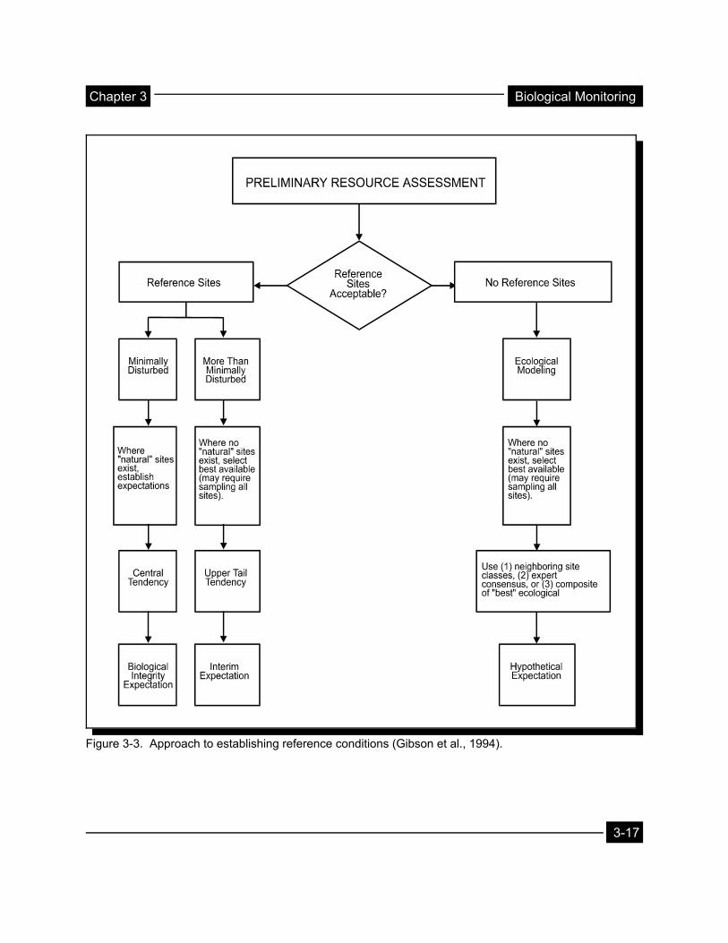
In a landscape that is heavily altered by agricultural activity, silviculture, industrial-commercial development, or urbanization, undisturbed streams or reaches might not exist and reference conditions might need to be determined based on best professional judgment of that which is likely attainable, historical records, or another means of estimation. The most appropriate approach to establishing reference conditions is to conduct a preliminary resource assessment to determine the feasibility of using reference sites (Figure 3-3). If acceptable, minimally impaired reference sites cannot be found for a region, some form of simulation modeling might be the best alternative. Biological attributes can be modeled from neighboring regional site classes, expert consensus, and/or a composite of “best” ecological information. Such models might be the only viable
means of examining significantly altered systems. The expectations derived from these models should be regarded as hypothetical until more reliable information is obtained.
3.5 RAPID BIOASSESSMENT PROTOCOLS
EPA has recommended a set of rapid bioassessment protocols, or RBPs, that use benthic macroinvertebrate and fish communities to assess biological condition in streams and wadable rivers. The five protocols differ in the level of effort, taxonomic level, and expertise required to perform them, and in the applicability of the data obtained (Table 3-2). More intensive bioassessments (RBPs III and V) give the most useful information for trend analysis and establishment of a baseline for problem diagnosis. RBPs I and II are less intensive bioassessment approaches and are useful for setting priorities for more intensive study. RBP IV, not described here, is a screening technique used to survey persons knowledgeable about the fish in an area. For further information about RBP IV, consult Plafkin et al. (1989).
Selection of appropriate organisms and protocols for biological assessment depends on the objectives of the monitoring study (Figure 3-4). RBP benthic protocols have been applied in freshwater streams and wadable rivers, and their applicability is presently limited to these waterbodies. Fish RBP protocols have been used in freshwater streams and larger rivers and are applicable to both. RBP-type methods for fish and invertebrates have been adapted for use by many states and federal agencies and are in use across the country (Southerland and Stribling, 1995).
3-16
Chapter 3 Biological Monitoring
Figure 3-3. Approach to establishing reference conditions (Gibson et al., 1994).
3-17

Biological Monitoring Chapter 3
Table 3-2. Five tiers of the rapid bioassessment protocols (Plafkin et al., 1989).
Level of Level
or Tier Organism
Group Relative Level
of Effort Taxonomy/Where
Performed Level of Expertise
Required
I benthic invertebrates
low; 1-2 hr per site (no standardized sampling)
order, family/field one highly trained biologist
II benthic invertebrates
intermediate; 1.5-2.5 hr per site (all taxonomy performed in field)
family/field one highly trained biologist and one technician
III benthic invertebrates
most rigorous; 3-5 hr per site (2-3 hr of total are for lab taxonomy)
genus or species/ laboratory
one highly trained biologist and one technician
IV fish low; 1-3 hr per site (no
fieldwork involved) not applicable one highly trained
biologist
V fish most rigorous; 2-7 hr per
site (1-2 hr per site are for data analysis)
species/ field one highly trained biologist and 1-2 technicians
3.6 THE MULTIMETRIC APPROACH FOR
BIOLOGICAL ASSESSMENT
Accurate assessment of biological condition requires a method that integrates biotic responses through an examination of patterns and processes from the organism to ecosystem level (Karr et al., 1986). The rapid bioassessment protocols (Plafkin et al., 1989) discussed above make use of an array of measures that individually provide information on diverse biological attributes and, when integrated, provide an overall indication of biological condition.
The raw biological data collected during a survey consist entirely of taxonomic identifications and numbers of individuals within each taxon. The level of identification—whether to family, genus, or species—depends on the method being used. For instance, RBP II involves identification to the
family level, whereas RBP III involves identification to the lowest practical level, generally genus or species. These data are used to calculate or enumerate a variety of values, or metrics. Each reflects a different characteristic of community structure and has a different range of sensitivity to pollution stress (Plafkin et al., 1989). Appropriately developed metrics can be used to draw conclusions about different aspects of the biological condition at a site, and measurements of multiple metrics in a biological assessment will yield a more accurate representation of the overall biological condition at a site. Gray (1989) stated that the three best-documented biological responses to environmental stressors are a reduction in species richness, a change in species composition to dominance by opportunistic species, and a reduction in the mean body size of organisms. Though the last type of biological response (change in mean body size) may be well
3-18

APPROACH Decide on Monitoring
Objectives
Determine whether an impairment
exists
Limited effort impairment noted
RBP I RBP IV
Determine if further
investigation is necessary
Determine the relative impact NPS
pollution
Define a WQ problem
Measure BMP
programeffectiveness
Assess compliance with WQS
Focus on communities. 3 levels of impairment
detected
Focus on communities and populations. 4
levels of Impairment detected
SCREENING MORE RIGOROUS APPROACHES
RBP II RBP III RBP V
Chapter 3 Biological Monitoring
Figure 3-4. Selection and application of the different tiers of RBP depend on monitoring objectives.
documented, it is rarely used in the more common bioassessment protocols because the level of effort for an accurate interpretation can be prohibitive.
Figure 3-5 illustrates a conceptual structure for the attributes calculated or measured for a biological assemblage during a biological assessment. Generally, the biological assemblage at a site can be characterized by metrics organized into four classes—community structure, taxonomic composition, individual condition, and biological processes. These are described below.
Community structure is characterized by measurements of the variety of taxa and the distribution of individuals among taxa. Taxa richness is the number of distinct taxa in a sample
and reflects the diversity of the sample. The relative abundance of each taxon is a comparison of the number of individuals in one taxon to the total number of individuals in the sample. Dominance is calculated as the percent composition of the dominant taxon within the total sample. It indicates balance within the community.
Taxonomic composition refers to the types of taxa in the sample. Sensitivity to pollution and other environmental disturbance is the number of pollution-tolerant and intolerant species in the sample. The presence of exotic and nuisance species is also noted because they can play important ecological roles and indicate stressed conditions.
3-19

Biological Monitoring Chapter 3
Individual condition is more easily measured in fish than in benthos and periphyton; it refers to the presence or absence and frequency of diseases and anomalies. Contaminant levels in the tissues of individuals can also be measured. The frequency of head capsule deformities in midges (Chironomidae) has been used by some researchers.
Biological processes occurring at the sample site are indicated by measurements of species that perform specific functions within the community. For instance, the functional feeding groups (e.g., detritivores, filter feeders) indicate the primary source of energy for the biological system.
Numerous biological metrics have been tested in various regions of the country (Figure 3-6), primarily for fish and benthos. Summaries of those used have recently been presented in tabular form (Gibson et al., 1996; Barbour et al., 1995) and are reproduced in Tables 3-13 and 3-14 at the end of this chapter. Examples of metrics that have been tested and have had scoring criteria established are those for the montane region of Wyoming (Table 3-3) and the plains streams of Florida (Table 3-4). Figure 3-1 explains five common metrics and presents sample data and calculated values for each of the metrics. Readers should calculate the metrics themselves to be certain that use of the data for metric calculation is understood.
3.7 SAMPLING CONSIDERATIONS
The large influence that small environmental factors, such as amount of sunlight or presence of woody debris in a waterbody, can have on aquatic communities means that even though there might not be easily distinguished boundaries between
habitats, such as those between riffles and pools, the biota inhabiting them are often taxonomically and biologically distinct (Hawkins et al., 1993). The distribution of benthic fauna in lakes and streams is also heterogeneous because of variable requirements among species for feeding, growth, and reproduction, which are satisfied for different species by different substrata, water chemistry, and inputs of woody debris (Wetzel, 1983). This leads to a patchy, nonrandom distribution of animals.
Because of the influence that habitat has on biological communities, sampling similar habitats at all sampling stations is important for data comparability and for data interpretation (Plafkin et al., 1989). Collection of habitat quality data each time biological data are collected helps to establish the correlation between the two for a particular ecoregion. Obviously, the more correlative data that are collected, the more useful they will be in interpreting sampling data, that is, in separating water quality and habitat quality effects as they relate to biological condition. The ability to separate the two influences is important for determining the expected or potential improvement in biological condition from water quality improvement programs such as point or nonpoint source pollution control (Barbour and Stribling, 1991).
When sampling multiple habitats, it is important to establish consistency in sampling procedures. Sampling protocols should be standardized, and the same level of effort should be applied at each sampling station. Because differences in gear efficiency and techniques may affect results, standardized sampling is needed if direct comparisons are to be made between stations or between data from a single station at different times.
3-20

Chapter 3 Biological Monitoring
Figure 3-5. Organizational structure of attributes that can serve as metrics.
3.7.1 Benthic Macroinvertebrate Sampling
Stream environments contain a variety of macro-and microhabitat types including pools, riffles, and runs of various substrate types; snags; and macrophyte beds. Relatively distinct assemblages of benthic macroinvertebrates inhabit various habitats (Hawkins et al., 1993), and it is unlikely that most sampling programs would have the time and resources to sample all habitat types. Decisions on the habitats selected for sampling should be made with consideration of the regional characteristics of the streams. For instance, high-gradient mountain streams are best sampled from
the cobble substrate of riffles for macroinvertebrates, whereas low-gradient coastal streams lack riffles and are appropriately sampled from snags and shorezone vegetation. These two different stream types might be sampled with different methods, during different times of the year, or with different biological index periods. The seasonal variability of the biota and stream environment are key factors that determine the proper index period. Established sampling protocols that are part of existing monitoring programs should be considered for NPS bioassessment. However, current and/or historical sampling approaches should be evaluated to determine whether they will provide the required data to address the program objectives.
3-21

Biological Monitoring Chapter 3
Figure 3-6. Areas in which various fish IBI metrics (see Table 3-4) have been used.
Sampling a single habitat, such as riffles, limits the variability inherent in sampling natural habitats. This can produce a more repeatable characterization of the biological condition of a stream because sampling bias is reduced, whereas sampling of multiple habitats must be carefully standardized to reduce investigator bias and to control for sampling efficiency problems.
If the biological assessment strategy is to sample a single habitat, the most representative stable habitat conducive to macroinvertebrate colonization should be chosen. The most suitable habitat choice will vary regionally. The key is to select one habitat that supports a similar assemblage for benthos within a range of stream sizes, is the most representative of the stream type or class under investigation, and is likely to reflect
anthropogenic disturbances within the watershed. Suitable habitat alternatives to riffles for sampling benthos include snags, downed trees, submerged aquatic vegetation beds, emergent shoreline vegetation, and the most prevalent substrate.
The RBPs recommended by EPA specify that a subsample of 100 organisms be used for a biological assessment; however, several states use 200 to 300 organisms or more. Agencies should evaluate the level of subsampling required to meet their objectives. The level of taxonomic identification should be specified in the study design and is determined by the study objectives. Identification to the species level gives the most accurate information on pollution tolerances and sensitivities, though some metrics or analytical techniques might require identification only to the
3-22

Chapter 3 Biological Monitoring
Table 3-3. Scoring criteria for the core metrics as determined by the 25th percentile of the metric values from the Middle Rockies-Central Ecoregion, Wyoming.
Metric
Stream Class Elevation > 6,500 ft Elevation < 6,500 ft
Score 5 3 1 5 3 1
EPT Taxa >14 14-8 <8 >18 18-10 <9
% Plecoptera >7% 7%-4% <4% - - -
% Ephemeroptera - - - >22% 22%-11% <11%
% Chironomidae <36% 36%-68% >68% >6% 6%-4% <4%
Predator Taxa >5 5-3 <3 <12% 12%-39% >39%
% Scrapers >5% 5%-3% <3% >7 7-4 <4
MHBI <4.3 4.3-4.8 >4.8 >8% 8%-5% <5%
BCI >74 74-42 <42 <3.7 3.7-4.7 >4.7
CTQD <99 99-112 >112 >79 79-46 <46
Shannon H >3.5 3.5-1.8 <1.8 - - -
% Multivoltine <48% 48%-57% >57% - - -
% Univoltine >40% 40%-20% <20% - - -
% Collector-Filterers - - - <2.6% 2.6-23.2 >23.2%
Range of Aggregate Score 11-55 9-45
order, family, or genus. Verification of taxonomic identifications is critical and can be accomplished by (1) comparing specimens with a reference specimen collection or (2) sending specimens to taxonomic experts familiar with the group in question.
Benthic macroinvertebrates can be collected actively or passively. Two of the more commonly used active methods use a square-meter kicknet or a long-handle D-frame. The former is typically used at sites that are considered to be in higher-gradient (riffle-prevalent) streams (Plafkin et al.,
1989); the latter is used primarily in coastal plains streams and is standardized as the 20-jab method (USEPA, 1997). In both of these methods, organisms are dislodged from their substrate by the sampler and captured in a net. Passive collection approaches include the Hester-Dendy multiplate sampler and rock baskets. These are considered artificial substrates. They are placed in the stream or stream bottom and left for a standardized amount of time. Upon retrieval, the invertebrates are removed from the sampling units in the laboratory. For further information on sampling methods, see Klemm et al. (1990).
3-23
Biological Monitoring Chapter 3
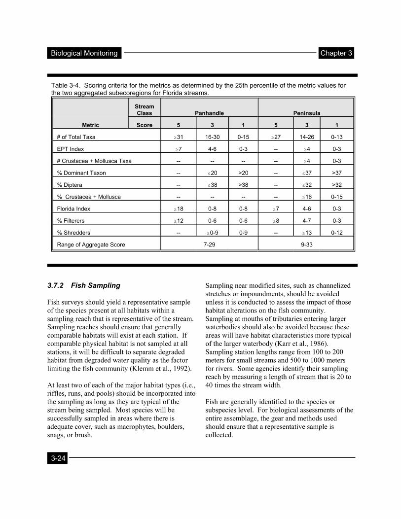
Table 3-4. Scoring criteria for the metrics as determined by the 25th percentile of the metric values for the two aggregated subecoregions for Florida streams.
Metric
Stream Class Panhandle Peninsula
Score 5 3 1 5 3 1
# of Total Taxa $31 16-30 0-15 $27 14-26 0-13
EPT Index $7 4-6 0-3 - $4 0-3
# Crustacea + Mollusca Taxa - - - - $4 0-3
% Dominant Taxon - #20 >20 - #37 >37
% Diptera - #38 >38 - #32 >32
% Crustacea + Mollusca - - - - $16 0-15
Florida Index $18 0-8 0-8 $7 4-6 0-3
% Filterers $12 0-6 0-6 $8 4-7 0-3
% Shredders - $0-9 0-9 - $13 0-12
Range of Aggregate Score 7-29 9-33
3.7.2 Fish Sampling
Fish surveys should yield a representative sample of the species present at all habitats within a sampling reach that is representative of the stream. Sampling reaches should ensure that generally comparable habitats will exist at each station. If comparable physical habitat is not sampled at all stations, it will be difficult to separate degraded habitat from degraded water quality as the factor limiting the fish community (Klemm et al., 1992).
At least two of each of the major habitat types (i.e., riffles, runs, and pools) should be incorporated into the sampling as long as they are typical of the stream being sampled. Most species will be successfully sampled in areas where there is adequate cover, such as macrophytes, boulders, snags, or brush.
Sampling near modified sites, such as channelized stretches or impoundments, should be avoided unless it is conducted to assess the impact of those habitat alterations on the fish community. Sampling at mouths of tributaries entering larger waterbodies should also be avoided because these areas will have habitat characteristics more typical of the larger waterbody (Karr et al., 1986). Sampling station lengths range from 100 to 200 meters for small streams and 500 to 1000 meters for rivers. Some agencies identify their sampling reach by measuring a length of stream that is 20 to 40 times the stream width.
Fish are generally identified to the species or subspecies level. For biological assessments of the entire assemblage, the gear and methods used should ensure that a representative sample is collected.
3-24

Chapter 3 Biological Monitoring
Fish can be collected actively or passively. Active collection methods involve the use of seines, trawls, electrofishing equipment, or hook and line. Passive collection can be conducted either by entanglement using gill nets, trammel nets, or tow nets, or by entrapment with hoop nets or traps. For a discussion on the advantages and limitations of the different gear types, see Klemm et al. (1992). The Index of Biotic Integrity (IBI) emphasizes active gear, and electrofishing is the most widely used active collection method. Ohio EPA (1987) discusses appropriate electrofishing techniques for bioassessment. Other sources for sampling method discussions are Allen et al. (1992), Dauble and Gray (1980), Dewey et al. (1989), Hayes (1983), Hubert (1983), Meador et al. (1993), and USFWS (1991).
Length and Weight Measurements
Length and weight measurements can provide estimations of growth, standing crop, and production of fish. The three most commonly used length measurements are standard length, fork length, and total length. Total length is the measurement most often used.
Age may be determined using the length-frequency method, which assumes that fish increase in size with age. However, this method is not considered reliable for aging fish beyond their second or third growing season. Length can also be converted to age by using a growth equation (Gulland, 1983).
Annulus formation is a commonly used method for aging fish. Annuli (bands formed on hard bony structures) form when fish go through differential growth patterns due to the seasonal temperature changes of the water. Scales are generally used for age determination, and each species of fish has a specific location on the body for scale removal that yields the clearest view for identifying the annuli. More information on the annulus formation method and most appropriate scale locations by
species can be found in Jerald (1983) and Weatherley (1972).
Fish External Anomalies
The physical appearance of fish usually indicates their general state of well-being and therefore gives a broad indication of the quality of their environment. Fish captured in a biological assessment should be examined to determine overall condition such as health (whether they appear emaciated or plump), occurrence of external anomalies, disease, parasites, fungus, reddening, lesions, eroded fins, tumors, and gill condition. Specimens may be retained for further laboratory analysis of internal organs and stomach contents if desired.
Periphyton
Of the three biological assemblages discussed in this chapter, periphyton is perhaps the least used, though the information potential can be dramatic as well as cost-effective. Laboratory analysis of species composition is labor-intensive. Because species within a genus can display varying tolerances to a disturbance, diatoms must be identified to species. Rosen (1995) estimates an average of 2 hours per sample to identify 500 organisms to species, with processing time decreasing as taxonomic expertise is gained.
Periphyton are a community of organisms that adhere to and form a surface coating on stones, plants, and other submerged objects. These can take the form of soft algae, algal or filamentous mats, or diatoms. As the primary producers in the stream ecosystem, their importance to the food web cannot be overstated. The advantages for using the periphyton assemblage in a bioassessment program are many:
• They have rapid reproduction rates and short life cycles and thus respond quickly to
3-25

Biological Monitoring Chapter 3
perturbation, which makes them valuable indicators of short-term impacts.
• Because they are primary producers and ubiquitous in all waters, they are directly affected by water quality.
• Periphyton sampling is rapid and requires few personnel, and results are easily quantified.
• A list of the taxa present and their proportionate abundance can be analyzed using several metrics or indices to determine biotic condition and diagnose specific stressors.
• The periphyton community contains a naturally high number of taxa that can usually be identified to species.
• Tolerance of or sensitivity to changes in environmental conditions are known for many species or assemblages of diatoms.
• Periphyton are sensitive to many abiotic
Network design refers to the array, or network, of sampling sites selected for a monitoring program. It usually takes one of two forms:
• Probabilistic design: Network that includes sampling sites selected randomly to provide an unbiased assessment of the condition of the waterbody at a scale above the individual site or stream; can address questions at multiple scales.
• Targeted design: Network that includes sampling sites selected based on known existing problems, knowledge of upcoming events in the watershed, or a surrounding area that will adversely affect the waterbody such as development or deforestation; or installation of BMPs or habitat restoration that is intended to improve waterbody quality; provides assessments of individual sites or reaches.
An integrated design combines these two approaches and incorporates multiple sampling scales and monitoring objectives.
factors that might not be detectable in the insect and fish assemblages.
The state of Kentucky has developed a Diatom Bioassessment Index (DBI), currently used in water quality assessments (Kentucky Department of Environmental Protection, 1993). Metrics use to construct the DBI include diatom species richness, species diversity, percent community similarity to reference sites, a pollution tolerance index, and percent sensitive species. Scores for each metric range from 1 to 5. The scores are then translated into descriptive site bioassessments, which are used to determine aquatic life use.
For diatoms, Montana (Bahls, 1993) uses a diversity index, a similarity index, and a siltation index. Three other metrics—dominant phylum, indicator taxa, and number of genera—are used for soft-bodied algae to support the diatom assessment.
3.8 BIOMONITORING PROGRAM DESIGN
The design of a biomonitoring program (similar to other types of monitoring programs) will depend ultimately on the goals and objectives of the program. Several of the objectives identified in Chapter 2 of this document can be directly addressed using a properly designed biomonitoring program. These objectives may differ in spatial and temporal scales, therefore requiring different monitoring designs as reflected in differences in the site selection process, number of sites sampled, and time and frequency of sampling. The sampling design used in nonpoint source biological monitoring consists of one of three types of network designs depending on the objectives of the programs—probabilistic, targeted, or integrated design. Objectives that are site-specific, such as
3-26

Chapter 3 Biological Monitoring
determining whether biological impairment exists at a given site, are addressed using a targeted monitoring design (Table 3-5). Objectives that address questions of large-scale status and trends, for example, require a probabilistic design. For many nonpoint source objectives (see Chapter 2), an integrated network monitoring design is most appropriate.
Monitoring performed at different spatial scales can provide different types of information on the quality and status of water resources. Conquest et al. (1994) discuss a hierarchical landscape classification system, originally developed by Cupp (1989) for drainage basins in Washington state, that provides an organizing framework for integrating data from diverse sources and at different resolution levels. The framework focuses on river and stream resources at its higher resolutions, but could be modified for other waterbody types such as lakes and wetlands. In its simplest form, the nested hierarchy consists of five levels:
• Ecoregions • Watersheds/subwatersheds • Valley segments • Habitat complexes (e.g., stream reach) • Habitat units (e.g., riffle)
Assessments of waterbodies on a large scale such as an ecoregion, subregion, state, or county provide information on the overall condition of waterbodies in the respective unit. Appropriately designed probabilistic sampling can provide results such as the percentage of waterbodies in a geographic area that are impaired (status), or, if the sampling is repeated at regular intervals, an assessment of the trends in the percentage of impaired waters. Probabilistic site selection is most appropriate for an unbiased estimate of the status and temporal behavior of waterbodies on a large geographic scale.
Assessments of waterbodies and subsequent monitoring often occur at the watershed scale, within which both targeted and probabilistic sites could be selected. A probabilistic design would yield information on the watershed scale as well as on the site- or stream-specific scale; these locations might or might not be impaired. The targeted design would ensure that known problem sites or sites of special interest are evaluated and their response over time is assessed.
Assessment on a small geographic scale may involve a whole stream, river, or bay or a segment (reach) of the waterbody. A targeted sampling design applies to monitoring waterbodies within a watershed that are exposed to known stressors. Known disturbances, such as point sources, specific NPS inputs, or urban stormwater runoff, can all be targeted for small-scale assessments. It is at this scale that the effectiveness of specific pollution controls, BMP installation/implementation, natural resource management activities, or physical habitat restoration can be monitored.
Since a target population is recognized to consist of groups that each have internal homogeneity (relative to other groups), it can be stratified to minimize within-group variance and maximize among-group variance (Gilbert, 1987). Table 3-6 summarizes a waterbody stratification hierarchy for streams and rivers, lakes, reservoirs, estuaries, wetlands, and ground water. With the exception of estuaries, the highest-level strata would be ecoregions and subecoregions. Biogeographic provinces (e.g., Virginian and Louisianian Provinces used in the Environmental Monitoring and Assessment Program (EMAP), as described by Weisberg et al. (1993)) are more appropriate as the highest stratification level for estuaries because of the relatively large size of their watersheds and the fact that they are influenced directly by marine processes.
3-27

Biological Monitoring Chapter 3
Table 3-5. Comparison of probabilistic and targeted monitoring designs.
Advantages Disadvantages
Probabilistic Design
Provides unbiased estimates of status for a valid assessment on a scale larger than that of the sample location.
Can provide large-scale assessment of status and trends of resource or geographic area that can be used to evaluate effectiveness of environmental management decisions for watersheds, counties, or states over time.
Stratified random sampling can improve sampling efficiency, provide separate data on each stratum, and enhance statistical test sensitivity by separating variance among strata from variance within strata.
Small-scale problems will not necessarily be identified unless the waterbody or site happens to be chosen in the random selection process.
Cannot track restoration progress at an individual site or site-specific management goals.
Stratified random sampling requires prior knowledge for delineating the strata (MacDonald et al., 1991).
Targeted Design
Systematic sampling along a stream or river can be an efficient means of detecting pollution sources (Gilbert, 1987).
Identifies small-scale status and trends of individual sites, which can be used to assess potential improvements due to restoration projects and other management activities.
Contributes to understanding of responses of biological resources to environmental impact.
A targeted design will not yield information on the condition of a large-scale area such as the watershed, county, state, or region. It cannot specifically monitor changes from management activities on a scale larger than site-specific.
Resource limitations usually make it impossible to monitor effects of all pollutant sources using a targeted design.
Systematic sampling can result in biased results if there is a systematic variation in the sampled population.
3-28

Chapter 3 Biological Monitoring
Depending on the waterbody, subsequent stratification levels may vary in number and may be quite different across waterbodies at a given level in the hierarchy. For example, a state or regional monitoring program designed to assess the status of biological communities in streams might need to be stratified to the level of segments, whereas monitoring to assess the efficacy of specific stream restoration measures might need to be stratified to the macro- or microhabitat level. If data collected by a particular design are so variable that meaningful conclusions cannot be drawn, poststratification of the data set might be required. If stratification to the level of microhabitat is needed, the sampling and analysis methods used at higher levels might be inappropriate or inadequate.
(2) Stratify the site classes. A sampling design appropriate to the monitoring objectives must be selected. For probabilistic designs, simple random sampling is not usually the optimal method. It can produce clusters of sampling sites that might not be representative of the larger scale area of interest (e.g., Hurlburt, 1984). Therefore, some sort of stratification is preferred for ensuring a dispersed distribution of site locations. Stratification can begin at an ecoregion site classification level and proceed to more specific levels of resolution as necessary to meet project objectives (Table 3-6). If there are clear clusters of differing land use among watersheds, the watersheds may be further stratified to ensure inclusion of an even distribution of land use types (e.g., subwatersheds having different levels of urban development). Waterbodies can be further stratified by section or segments. For instance, streams can be stratified by stream order (first, second, third, etc.), size of drainage area, or specific sections of a bay or lake.
3.8.1 Process of Randomized Sampling Site Selection
Probabilistic sampling designs require the random selection of sampling sites within the basic design (e.g., simple random, stratified random, multistage; Chapter 4). Three major steps are involved in selecting sampling sites using a probabilistic design:
(1) Identify the level of site classification. Monitoring program objectives will dictate the geographic extent to which monitoring is to be done, for instance statewide, county-wide, within an ecoregion, or within a watershed. This level of site classification should be identified initially.
(3) Select sampling sites. Sampling units or sites within each stratum (or other delineation as dictated by the general design) are randomly selected. This approach provides a basis for making general statements about the condition of the entire stratum, including sites not sampled.
3-29

Biological Monitoring Chapter 3
Tab
le 3
-6.
Wat
erbo
dy s
trat
ifica
tion
hier
arch
y.
Po
pu
lati
on
of
Inte
rest
S
trea
ms
and
Riv
ersa
Lak
es b
, c
Res
ervo
irs
b, d
E
stu
arie
s e
Wet
lan
ds
f G
rou
nd
Wat
er g
Ope
ratio
nal
Sam
plin
gU
nit (
SU
)
Cha
nnel
segm
ent (
i.e.,
a le
ngth
of
river
cha
nnel
into
whi
ch n
otr
ibut
arie
sflo
w)
Sel
f-co
ntai
ned
basi
n
Sel
f-co
ntai
ned
basi
n(h
ydro
logi
cally
isol
ated
from
oth
erba
sins
)
Sel
f-co
ntai
ned
basi
n T
rans
ect
upla
nd o
r de
ep w
ater
boun
darie
s
Tra
nsec
t
Str
ata
(or
high
erst
ages
)co
mpr
isin
gS
us
Eco
regi
on
Eco
regi
on
Eco
regi
on
Bio
geog
raph
icpr
ovin
ce
Wet
land
sys
tem
type
(mar
ine,
est
uarin
e, r
iver
ine,
lacu
strin
e, p
alus
trin
e)
Eco
regi
on
Wat
ersh
ed
Siz
e/su
rfac
e ar
eaof
lake
(km
2 )
Siz
e/su
rfac
e ar
eaof
res
ervo
ir (k
m2 )
[wat
ersh
edar
ea/b
asin
sur
face
area
]
Wat
ersh
ed
Wat
ersh
edre
char
ge, d
isch
arge
or
both
W
ater
shed
Str
eam
/riv
erch
anne
l(o
rdin
al/
area
l)
Lake
hydr
olog
y(r
eten
tion
time,
ther
mal
stra
tific
atio
n)
Hyd
rolo
gy (
wat
erle
vel f
luct
uatio
n/dr
awdo
wn;
rete
ntio
n tim
est
ratif
icat
ion)
Wat
ersh
edar
ea (
km2 )
Cla
ss (
base
d on
veg
etat
ive
type
; sub
stra
te a
nd fl
oodi
ngre
gim
e; h
ydro
perio
d)
Aqu
ifer
type
(unc
onfin
ed (
wat
erta
ble)
aqu
ifers
,co
nfin
ed (
arte
sian
wel
l) aq
uife
rs)
Seg
men
t C
hara
cter
istic
wat
er q
ualit
y(n
atur
alco
nditi
ons)
Cha
ract
eris
ticw
ater
qua
lity
(nat
ural
cond
ition
s)
Zon
es (
tidal
basi
n, d
epth
,sa
linity
)
Flo
odin
g re
gim
ew
ater
che
mis
try
soil
type
Aqu
ifer
mat
eria
lty
pe (
sedi
men
tary
rock
; mar
l;un
cons
olid
ated
rock
, et
c.)
Cha
ract
eris
ticw
ater
qua
lity
(nat
ural
cond
ition
s)
Hyd
raul
icco
nduc
tivity
(hom
ogen
eous
,he
tero
gene
ous,
isot
ropi
c,an
isot
ropi
c)
3-30

Chapter 3 Biological Monitoring
Tab
le 3
-6.
(con
tinue
d)
Po
pu
lati
on
of
Inte
rest
S
trea
ms
and
Riv
ersa
Lak
es b
, c
Res
ervo
irs
b, d
E
stu
arie
s e
Wet
lan
ds
f G
rou
nd
Wat
er g
Hab
itats
with
in S
us
Mac
roha
bita
t(p
ool/r
iffle
;sh
orez
one
vege
tatio
n;su
bmer
ged
aqua
ticm
acro
phyt
es)
Long
itudi
nal z
one
(riv
erin
e; tr
ansi
tiona
l;la
cust
rine;
tailw
ater
s(c
an b
e m
ore
river
ine
but a
lway
sas
soci
ated
with
dam
s))
Dep
th z
one
Dep
th z
one
(eul
ittor
al 6
prof
unda
l)
Dep
th
Sub
stra
te/h
abita
t S
ubsy
stem
(su
btid
al,
inte
rtid
al, t
idal
, low
erpe
renn
ial,
uppe
r pe
renn
ial,
inte
rmitt
ent,
litto
ral,
limne
tic)
Tem
pera
ture
Mic
roha
bita
t S
ubst
rate
/m
icro
habi
tat
Sub
stra
te/
mic
roha
bita
t S
ubst
rate
/ mic
roha
bita
t
a F
risse
ll et
al.,
198
6; b G
errit
sen
et a
l., 1
996
[Dra
ft]; c W
etze
l, 19
75; d T
horn
ton
et a
l., 1
990;
e Day
et a
l., 1
989;
f Cow
ardi
n et
al.,
197
9;g
Hea
th,
1989
.
3-31
Biological Monitoring Chapter 3
3.8.2 Targeted Site Selection
In a targeted site selection design, sites are selected based on the location of known or suspected perturbations (stressors), planned point source controls, or BMPs in the geographic area of concern. NPDES permits, urban stormwater sites, timber harvest areas, rangeland, row crop farming, construction sites, and Superfund sites are all examples of known stressor sites. Upstream/downstream sampling stations, beforeand-after site alterations, or recovery zones (sampling at established distances from sources) are types of sampling locations for known stressor sites. Ecologically sensitive sites that may or may not be affected by stressors might also be chosen as targeted sites.
3.8.3 Integrated Network Design
Integrated network design consists of integrating multiple monitoring subprograms to effectively meet various monitoring objectives and improve the applicability of data. An emerging biological monitoring program in Prince George’s County, Maryland, is used here as a useful example demonstrating the design components reviewed above (see box on next page).
Prince George’s County is interested in assessing the status and trends of biological stream resources in the county with known confidence. Assessment levels include county-wide, watershed-wide, and stream-specific. Biological assessment, based on sampling benthic macroinvertebrates, is used as the indicator of stream condition. Judgment of impairment or nonimpairment results from comparison to reference conditions (see Section 3.4). Two major components of this program are volunteer monitoring of selected sites and non-volunteer monitoring of probability-based and targeted sites. The volunteer sites serve for public
education and some initial screening of stream conditions. Those sites monitored by the non-volunteer program are intended to provide unbiased estimates of biological status of streams throughout the county, trends in their condition, problem identification, evaluation of management activities (e.g., restoration, BMP installation, chemical controls, and altered land use practices), and data for eventual establishment of cause-and-effect associations.
Three types of sites are monitored in this program to address the county’s multiple goals: targeted sites, reference sites, and probability sites. Each site type addresses specific questions on stream status in Prince George’s County. Targeted sites are sampled semiannually during two program index periods—spring and fall. Annual sampling allows estimation of intra- and interannual variation in the measured variables and indices, and it allows estimation of trends after several years of monitoring. After the first 2 or 3 years of monitoring, the data will be reevaluated to determine whether sampling at longer intervals (for example, every other year) is sufficient to detect trends. Data from targeted sites can document the decline or recovery of streams subject to specific stresses and will allow assessment of restoration and mitigation efforts.
A set of 15 to 20 reference sites (having over 50 percent forest cover) are monitored semiannually as are the targeted sites. These data allow estimation of annual variation and trends in the biological characteristics of the reference sites. These estimates are critical for determining the biological status of test sites.
Forty-one watersheds have been identified to address status and trends for the county. Site selection is in two stages. In the first stage, a set of watersheds are selected randomly. In the second
3-32

Chapter 3 Biological Monitoring
Case Study
Development of an Integrated Biological Monitoring and Assessment Program
in Prince George’s County, Maryland
Prince George’s County, Maryland, immediately east of Washington, DC, is developing a biological monitoring program to assess the status and trends in ecological condition and the physical habitat quality in county streams. Program goals include:
• Document and monitor the biological status and trends of county streams. • Integrate data from biological, chemical, and physical monitoring programs to make a
comprehensive assessment of the county’s stream resources. • Use biological monitoring data to identify and characterize impairment to the ecological system. • Further public education in environmental problems through a component of the biological
monitoring program tailored for layperson involvement. • Evaluate the effectiveness of environmental management and mitigation activities.
The program design includes both probabilistic and targeted elements that will allow specific questions to be addressed at three spatial scales—county-wide, watershed-wide, and stream-specific. Approximately 100 sampling locations have been selected for the initial year of monitoring (1995). In two separate sampling periods (early spring and fall), approximately 50 probability sites, 20 known problem sites, 20 reference sites, and another 15 sites will be used for either confirmation of volunteer monitoring results or quality control samples.
The sampling units are stream segments between confluences. Segments are sampled at accessible points. Sampling is two-stage: for the first stage, watersheds are selected randomly so that one-fifth of the watersheds in the county are sampled in any one year and all watersheds will be sampled in the fifth year of the program. The second stage is random selection of stream segments within watersheds, stratified by stream order, so that sampling effort is allocated optimally among three stream orders.
Used by permission of Watershed Protection Branch, Department of Environmental Resources, Prince George’s County, Maryland.
stage, stream segments within the selected watersheds are chosen at random for sampling. In each year of the monitoring program, a set of 6 to 10 watersheds are selected (depending on size) and approximately 45 stream segments of those watersheds are sampled. After 5 years, all watersheds in the county will have been sampled, and in the sixth year the program will return to the originally sampled watersheds. An estimate of status can be made for each watershed every 5
years. The status of streams county-wide can be estimated from the first year on. The first year’s estimate will be based on a small sample of watersheds and segments and will have greater uncertainty than the estimates developed in later years.
Prior knowledge of land use in the county was applied to stratify watersheds and sites. Urbanization is known to affect stream hydrology,
3-33
Biological Monitoring Chapter 3
water quality, habitat, and biota, and the northern watersheds of the county are urban and suburban, being close to Washington, DC. Therefore, Prince George’s County was divided (stratified) into northern and southern watersheds so that in any given year, an equal number of watersheds would be selected in the more urban north and in the more rural southern parts.
3.9 MONITORING TRENDS IN BIOLOGICAL
CONDITION
Two separate factors affect our ability to distinguish trends over time in biological monitoring. The first factor, common to any trend analysis, are those sources of variability inherent in the measurements obtained from the monitoring sites. A significant challenge is distinguishing random changes in biological monitoring data over time from actual trends. Section 4.4 outlines statistical considerations regarding this issue, and Figures 4-4 to 4-7 illustrate several common types of data patterns that might be obtained over time in a water quality monitoring program. One of the solutions to this challenge is to have either a long time series of data or a sufficient number of monitoring sites (probabilistic, targeted, or integrated design) so that the data can be statistically evaluated.
A second factor affecting the ability to detect trends in a biomonitoring program is the observed relationship between reference site data and monitoring site data over time. This factor is somewhat unique to biomonitoring programs because a biological assessment at any given time is dependent on data from two sources—the population of reference sites and the monitoring sites. Thus, an accurate interpretation of trends in a biological monitoring nonpoint source program is
accomplished, in part, by using a comparative analysis of reference site and monitoring site data. Figure 3-7 illustrates some possible trends that could be observed in a biological monitoring program. These types of data can be analyzed in a variety of ways as described in Section 4.4 and in Green (1993) and Smith et al. (1988).
Accurate characterization of trends in biological data over time depends on the degree to which sources of variability in the data are defined and characterized. In general, there are two major sources of variability—natural and experimental. Natural sources of variation include seasonal effects such as species life cycles, natural disturbances such as floods and fires, and microhabitat differences among sites or over time. Experimental sources of variability include collection method and gear variation. The previous discussion of biological assessment methods in this chapter addresses many of the common natural and experimental sources of variability. All field collection methods should be documented and standardized in approved SOPs. The use of a well-defined and appropriate field collection method, for example, reduces experimental sources of variability. Incorporation of a population of ecoregional reference sites into a biological monitoring design serves as a control for natural sources of variability over time, in addition to providing a sound data assessment framework. An apparently downward trend for certain sites in watersheds over time, for example, may be open to interpretation if the same trend is observed in reference sites (Figure 3-7). Repeated sampling during the same index period over time also provides some control for natural sources of variability.
3-34

Chapter 3 Biological Monitoring
YEAR
Inve
rteb
rate
Co
mm
un
ity
Ind
ex (
ICI)
Impa
ired
Nonim
paire
d
1977 1978 1979 1980 1982 1983 1984 1985 1986 1987 1988 1989 1990 1991 0
10
20
30
40
50
Figure 3-7. Some trends that might be observed during the course of a biological monitoring program.
Although natural sources of variability are not often amenable to characterization, experimental or method-sources of variation can and should be defined. Factors such as precision and sensitivity of the assessment scores are achieved by collecting and analyzing multiple samples from the same site using consistent procedures and by sampling and analyzing samples from multiple sites that are similar, particularly ecoregional reference sites. One of the results of this method characterization process is the ability to define the statistical power of a sampling and bioassessment method. Statistical power is the degree to which a Type 2 error has a given probability of occurrence. Put simply, this is the probability of assessing a site as unimpaired when in fact it is impaired; or concluding that there is no trend or change in water quality over time when in fact there has been a change.
Defining the statistical power of a given bioassessment method allows one to rigorously determine the number of sites necessary in a monitoring program to detect a given level of impairment, or a certain trend over time, with a known degree of confidence. A power analysis achieves this objective by constructing an empirical relationship between the number of sites or measurements observed and the resultant difference in assessment score detected between the reference and test sites. A bioassessment method that has substantial intra-site variability will have reduced statistical power resulting in a greater number of sampling sites to distinguish a given level of impairment. Similarly, a very heterogeneous population of ecoregional reference sites, with widely ranging bioassessment scores, will also yield reduced statistical power.
3-35

Biological Monitoring Chapter 3
An example of power analysis is shown for the Delaware coastal plain streams in which the benthic macroinvertebrate community was the biomonitoring indicator used to detect status and trends of water quality (Maxted and Dickey 1993; Figure 3-8). The power analysis graph shows a steep decline in the number of monitoring sites necessary as percent difference in assessment score (between reference and monitoring sites) decreases. In other words, if one is interested in detecting a
relatively small difference in assessment score between the reference and monitoring sites or if, alternatively, one wants to detect a relatively small change in assessment score over time with a high degree of confidence, a greater number of monitoring sites within a stratum (i.e., stream order, urban versus agricultural) will need to be sampled.
Determining the Appropriate Sampling Effort: An Example Using DNREC Data from the Mid-Atlantic Coastal Plain Ecoregion
Most environmental monitoring programs are designed to avoid detecting a problem or noncompliance that does not really exist. These false positives are called Type I errors. It is traditional to accept a 5 percent probability of false positives as occurring (see Section 4.1 for further discussion). The probability of false negatives (Type II error, failing to detect a problem that does exist) is evaluated through power analysis. A power analysis provides an estimate of the number of measurements (sample size) required to detect a change for a given significance level (usually, % = 0.05), with the power typically set at 80 percent. Power analysis requires prior knowledge of, or rational assumptions on, the statistical properties of the data, in particular, the nature of the variability associated with them. Two types of variance are used in power analysis: variance of total bioassessment scores among all reference sites and variance among total bioassessment scores within a site.
Maxted and Dickey (1993), as part of their nonpoint source biological monitoring program, produced replicated bioassessment data from 23 sites. Total bioassessment scores were developed for each using an RBP - type approach for normalization of six metrics: (1) taxa richness, (2) EPT index, (3) percent EPT abundance, (4) percent Chironomidae abundance, (5) percent dominant family, and (6) family biotic index.
The sampling error takes into account the natural variability among multiple sites; measurement error is the variability observed among multiple samples at the same site, that is, it tells us how well the site is being characterized. The power analysis estimates the number of samples required for a given percent difference in total bioassessment score. Using the sampling error, it estimated that in order to detect a 20 percent difference in the index value (between a population of reference sites and a population of test sites) a minimum of eight reference and eight test sites (subjected to NPS pollution) should be sampled (solid line in accompanying figure). Power analysis using the measurement error indicates that three repeated measurements at each site are necessary to detect a 20 percent difference in total bioassessment score (broken line in the accompanying figure).
Figure 3-8. Sample power analysis of a bioassessment method.
3-36

Chapter 3 Biological Monitoring
Figure 3-8. (continued)
3-37

Biological Monitoring Chapter 3
The Prince George’s County case study reviewed earlier illustrates how power analysis was used to determine the number of monitoring sites needed to obtain meaningful biomonitoring data. A design consideration was that impairment, as defined by a 50 percent reduction of the reference condition, be detected with 80 percent probability of detection, and 95 percent confidence that observed differences are significant. Power analysis (Fiugre 3-8) revealed that a sample of two sites on a stream class could be used to detect a difference of 50 percent using bioassessment procedures in coastal plain streams. Assessment of a single watershed can be done by sampling at least two sites of each stream order present in the watershed. Most of the 41 watersheds in this county are third-order coastal plain streams. Therefore, an average of 6 sites per watershed, or approximately 246 sites, should be sampled for an assessment of all watersheds. This represents approximately 25 percent of the total population of stream segments in the county.
The above considerations led to the target sampling design of 25 percent of stream segments. Because county-wide assessment is one of the goals of this program, selection probability was kept at 25 percent. The sampling rule used in this program is at least 25 percent of stream segments in each stream order are selected in each watershed. For example, one segment is selected if there are one to four segments of a given order in the watershed, two segments are selected if there are five to eight, and so on. The probability that a watershed will be included in sampling thus varies slightly among watersheds, and this probability is used as a weighting factor in county-wide assessment and estimation. Given an annual sampling effort of approximately 50 probability sites per year, a 5year rotation of sampling will allow assessment of all watersheds over the 5-year period.
Repeated sampling of monitoring and reference sites over time, along with adequate characterization of bioassessment method precision, can yield significant management information as demonstrated by the Ohio EPA bioassessment program. Since 1977, Ohio EPA (1992) has used assessments of the benthic macroinvertebrate assemblage to document changes in the biological condition of a waterbody. Figure 3-7 illustrates annual results of biological assessments using the Invertebrate Community Index (ICI) (Ohio EPA, 1992) over a 14-year period in the Cuyahoga River. A 95 percent confidence interval of ±4 ICI units was determined based on analysis of intra- and inter-site variance in ecoregional reference scores. The graph demonstrates several features, including a general improvement in water quality over time. Furthermore, certain apparent changes in score between 1977 and 1980 are in fact illusory since the confidence intervals overlap. Thus, actual trends can be statistically differentiated from random changes in the data over time.
3.10 OVERVIEW OF SOME STATE PROGRAMS
Biological monitoring programs of five states are highlighted to illustrate technical components of biological monitoring programs, which are summarized for nonpoint source evaluations in Table 3-7. The Delaware Department of Natural Resources and Environmental Conservation (DNREC) led the Mid-Atlantic Coastal Streams (MACS) workgroup in adapting the RBPs to low-gradient streams. The MACS workgroup consists of technical staff from biomonitoring programs of Delaware, Maryland, Virginia, and North Carolina (USEPA, 1997). They were able to determine that the most appropriate method for obtaining a representative
3-38

Chapter 3 Biological Monitoring
Table 3-7. Summary of the primary technical issues related to biological monitoring for nonpoint source evaluations.
Biomonitoring for Nonpoint-source Evaluations
Sampling Area/ Size
Sampling is conducted over a stream reach, such that a composite of different habitats or different parts of a habitat is created. Natural biological heterogeneity is accounted for by sampling a relatively large area. Fish sampling may extend from 100 yards to 20 or 30 times the stream width. Benthic sampling may extend over several riffles or a composite of habitats taken from a 100-yard length of stream.
Replication
Replication at a site is important to evaluate within-site variability. However, several samples taken at a single site would be pseudoreplication if used to evaluate effects of impacts, such as nonpoint source pollution. Sites from different streams and watersheds are considered replicates to assess status or condition of regions or watershed basins. Monitoring can be accomplished with single large samples that sufficiently represent the stream reach under study.
Sampling Gear
Gear can be as rigorous and quantitative as a program deems necessary. However, gear must efficiently sample the targeted assemblage and specified habitat and be maintained in good operational condition. Electrofishing is the preferred gear for fish assemblages. Most state agencies have selected a kick seine or D-frame, and artificial substrates are used for periphyton.
Biological Index Period
The investigator must find a compromise between selecting a sampling period that is representative of the biological community and selecting one that reflects the worst-case conditions of pollutant stress. Seasonality is an important consideration because the taxonomic and functional feeding group compositions change naturally throughout the year in response to emergence and reproductive cycles. The optimal biological index period will vary throughout the United States. Some states, such as Florida, have more than one index period for sampling.
sample of benthic macroinvertebrates from low-gradient, sandy-bottomed, coastal plain streams was a multihabitat approach. The approach uses a standard D-frame net and samples the most dominant habitat types from a 100-meter reach in proportion to their frequency. The Delaware DNREC samples approximately 300 sites on an annual basis using this approach (Table 3-8). The Florida Department of Environmental Protection
has adopted this method for its nonpoint source monitoring program (Table 3-9) and has established reference conditions. The State of Montana, Department of Health and Environmental Sciences, uses a different approach for its higher-gradient streams, which are generally cobble-bottomed (Table 3-10). It has adapted a traveling kick method for macroinvertebrates and is developing reference conditions. The health of
3-39

Biological Monitoring Chapter 3
Table 3-8. Selected biomonitoring program components, Delaware Department of Natural Resources and Environmental Conservation (DNREC).
Macroinvertebrates
Habitat Selection
Stable habitats that are 5% of the 100-meter assessment area. Habitats include snags, submerged macrophytes, banks/root systems, and riffles. Sampled in proportion to representation.
Sample Gear/ Preservation
Standard aquatic D-frame dip net (0.3-meter width, 700- to 900-micron mesh), sieve bucket (600-micron mesh), 70% ethanol, storage containers (1- to 2-liter).
Sampling Method
20-jab method; a single jab consists of thrusting the net into a productive habitat for a distance of approximately 1 meter. 20 jabs composited across habitats (6.2 m2). Samples are cleaned by running stream water through the net, then transferring to a sieve bucket for further cleaning. Transferred to a storage container and preserved in 70% ethanol.
Subsampling and Enumeration
Preserved samples returned to the lab for processing. Subsampling to 100-organism level.
Taxonomic Level Currently at family level. Investigating efficacy of doing genus-level identifications.
QA procedures Same as RBPs (Plafkin et al., 1989); habitat assessments are evaluated by all investigators while reviewing the slides and field notes. Field investigators must have proper training.
Habitat Assessment
Field data sheet: 7 parameters numerically scored (1-20) similar to RBPs; documents other physical and water quality data.
Comments Standard operating procedures in draft form and prepared by Mid-Atlantic Coastal Streams Workgroup.
the fish assemblage is the primary biological monitoring indicator for the North Dakota Department of Environmental Health (Table 3-11), which is planning to further develop its monitoring program to include benthic macroinvertebrates. The State of Vermont, Department of
Environmental Conservation, does three types of sampling (Table 3-12)—fish, benthic macroinvertebrates from riffles in high-gradient streams, and benthic macroinvertebrates from multihabitats in low-gradient streams.
3-40

Chapter 3 Biological Monitoring
Table 3-9. Selected biomonitoring program components, Florida Department of Environmental Protection (Florida DEP).
Macroinvertebrates
Habitat Selection
Presence or absence of major productive habitats at each sampling location is established during preliminary reconnaissance. Habitats include: riffles, snags, aquatic vegetation, leaf packs, undercut banks/root systems, leaf mat, rocky outcrops, muck/silt, sand. Major habitats sampled equally; Group of minor habitats treated as a single major habitat.
Sample Gear/ Preservative
Standard D frame dip net (0.3 meter width 600 micron mesh), wide mouth jars, formalin.
Sampling Method 20 jab dip net sample, composite sample across habitats. Individual jabs are approximately 0.5 m making a total composite of 3 m2 .
Subsampling and Enumeration
Entire sample in gridded pan (5 X 3 cm grids), randomly select grids (1/72 of sample), remove contents, sort into taxonomic groups, continue until a minimum of 100 organism are counted; a grid’s entire contents must be sorted.
Taxonomic Level Lowest taxonomic level (genus or species).
QA Procedures Replicate sampling for 10% of samples collected on an annual basis have not been implemented but are planned. Resorting of 10% of samples. Field crew undergo periodic training.
Habitat Assessment
Field data sheet, 7 visually-estimated habitat parameters, weighted equally. Physical/Chemical characterization field data sheet
Comments
Stream classification factors for establishing reference conditions based on Ecoregion and subecoregion. Site selection factors: Availability of least impaired and reference sites, specific monitoring issues, accessibility and safety, compatibility of habitat. Standard operating procedures and report describing state-wide nonpoint source program prepared by Florida DEP and support contractors.
3-41

Biological Monitoring Chapter 3
Table 3-10. Selected biomonitoring program components, Montana Department of Health and Environmental Sciences (Montana DHES).
Macroinvertebrates
Region of State Entire
Site Selection Riffles
Sample Gear 12-inch D-frame net
Sampling Method Travelling kick across riffles, 1-2 diagonal collections (time and distance recorded)
Subsampling and Enumeration
300-organism subsample in laboratory
Taxonomic Level Genus/species
QA Procedures Replication on selected sites and projects
Habitat Assessment
Follows RBP habitat assessment approach
Comments Lab processing done by outside contractors
3-42

Chapter 3 Biological Monitoring
Table 3-11. Selected biomonitoring program components, North Dakota Department of Environmental Health (North Dakota DEH).
Macroinvertebrates Fish
Region of State Not developed as of current date Red River
Site Selection 25 sites to date; randomized selection, but dictated by access logistics
Sample Gear Electrofishing; shore-based longline
Sampling Method Minimum of 100 meters; 20 times river width on wide rivers
Subsampling and Enumeration
Not applicable
Taxonomic Level Lowest positive taxon
QA Procedures 10 percent repeat sampling
Habitat Assessment
Based on RBPs
Comments Planned to be started in 1997 In development
3-43

Biological Monitoring Chapter 3
Table 3-12. Selected biomonitoring program components, Vermont Department of Environmental Conservation (Vermont DEC).
Macroinvertebrates Fish
Region of State Entire state; high gradient
Entire state; low gradient
Entire state
Site Selection Riffles Woody debris Macrophytes Boulders
Representative of reach; mix of riffle, run, pool
Sample Gear Rectangular kick net 18 in x 8 in 500-µm mesh
Rectangular kick net 18 in x 8 in 500-µm mesh
Electro-shocking
Sampling Method
2-min timed composite; 30 sec in each of 2 points in slow area; 2 points in fast area
2-min sample; all substrate materials are hand scrubbed
1-3 upstream passes into blocknet or vertical drop instream
Sub-sampling and Enumeration
Preserve in field; subsample gridded tray 1/4 sample and min 300 animals
Preserve in field subsample gridded tray (technique allows density estimate for site)
Total count
Taxonomic Level Specified in protocols; family-genus-species, depending on order
Protocols list taxonomic level and key to be used
Species
QA Procedures
All samples archived; replicate samples always collected; two people check pick; two people trained in each taxonomic order
All samples archived; replicate samples always collected; two people check pick; two people trained in each taxonomic order
Same person conducts collection and taxonomy
3-44

Chapter 3 Biological Monitoring
Table 3-12. (continued)
Macroinvertebrates Fish
Habitat Assessment
Includes substrate composition, embeddedness, periphyton cover type, canopy cover, immediate riparian zone info ave. stream velocity, depth
Includes substrate composition, embeddedness, periphyton cover type, canopy cover, immediate riparian zone information, average stream velocity, depth
Qualitative or quantitative transect method; depth, velocity, substrate
Comments
Also record temperature, pH, alkalinity, condition and characterization of site, elevation, DO; also will look at stream low flow characteristics and surficial and bedrock geology and land use cover to help differentiate sites as “ecotype”; set biocriteria for individual metrics
Has modified the Index of Biotic Integrity to fit Vermont’s wadable streams
3-45

Biological Monitoring Chapter 3
Tab
le 3
-13.
Fis
h In
dex
of B
iotic
Inte
grity
met
rics
used
in v
ario
us r
egio
ns o
f Nor
th A
mer
ica.
Alte
rnat
ive
IBI m
etric
s M
etric
Cat
egor
y M
idw
est
New
Eng
land
O
ntar
io
Cen
tral
App
alac
hia
Col
orad
oFr
ont R
ange
W
este
rnO
rego
n Sa
cram
ento
-Sa
n Jo
aqui
n W
isco
nsin
1.
Tota
l num
ber o
f spe
cies
A
X
# N
ativ
e fis
h sp
ecie
s A
X X
# Sa
lmon
id a
ge c
lass
esa
A
2.
Num
ber o
f dar
ter s
peci
es
B X
# Sc
ulpi
n sp
ecie
s B
# Be
nthi
c in
sect
ivor
e sp
ecie
s B
# D
arte
r and
scu
lpin
spe
cies
B
X
# Sa
lmon
id y
earli
ngs
(indi
vidu
als)
a B
% R
ound
-bod
ied
suck
ers
B X
# Sc
ulpi
ns (i
ndiv
idua
ls)
B
3.
Num
ber o
f sun
fish
spec
ies
B X
X
# C
yprin
id s
peci
es
B
# W
ater
col
umn
spec
ies
B
# Su
nfis
h an
d tro
ut s
peci
es
B
# Sa
lmon
id s
peci
es
B
# H
eadw
ater
spe
cies
B
X
4.
Num
ber o
f suc
ker s
peci
es
B X
X
# Ad
ult t
rout
spe
cies
a B
# M
inno
w s
peci
es
B X
# Su
cker
and
cat
fish
spec
ies
B
5.
Num
ber o
f int
oler
ant s
peci
es
B X
X
# Se
nsiti
ve s
peci
es
B X
Pres
ence
of b
rook
trou
t B
X X
X X
X X
X X
X X
X
X X X
X X
X
X
X
X
X
X X X
X
X
X
X X
X
X
3-46
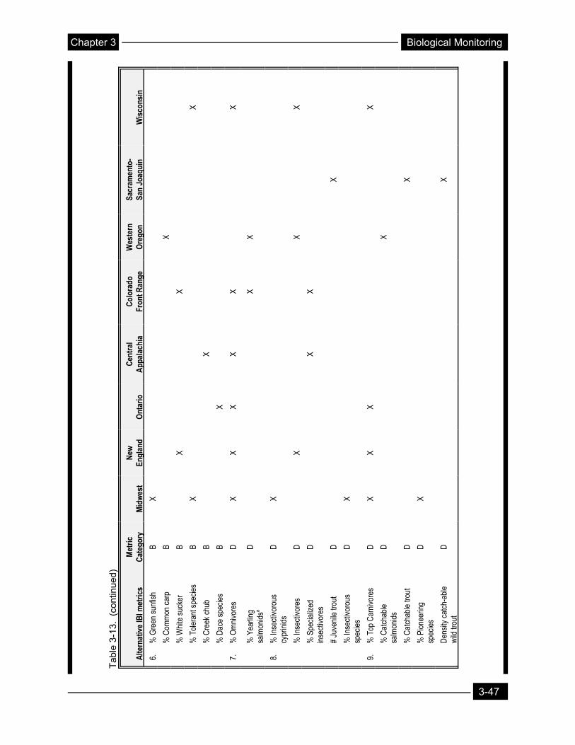
Chapter 3 Biological Monitoring
Tab
le 3
-13.
(co
ntin
ued)
Met
ricN
ewC
entr
alC
olor
ado
Wes
tern
Sacr
amen
to-
Alte
rnat
ive
IBI m
etric
s C
ateg
ory
Mid
wes
t En
glan
d O
ntar
io
App
alac
hia
Fron
t Ran
ge
Ore
gon
San
Joaq
uin
Wis
cons
in
6.
% G
reen
sun
fish
B X
% C
omm
on c
arp
B X
% W
hite
suc
ker
B X
X
% T
oler
ant s
peci
es
B X
X
% C
reek
chu
b B
X
% D
ace
spec
ies
B X
7.
% O
mni
vore
s D
X
XX
X X
X
% Y
earli
ngD
X
X
sa
lmon
idsa
8.
% In
sect
ivor
ous
D
X
cypr
inid
s
% In
sect
ivor
es
D
X X
X
% S
peci
aliz
edD
X
X in
sect
ivor
es
# Ju
veni
le tr
out
D
X
% In
sect
ivor
ous
D
X
spec
ies
9.
% T
op C
arni
vore
s D
X
X X
X
% C
atch
able
D
X
salm
onid
s
% C
atch
able
trou
t D
X
% P
ione
erin
gD
X
sp
ecie
s
Den
sity
cat
ch-a
ble
D
X
wild
trou
t
3-47

Biological Monitoring Chapter 3
Tab
le 3
-13.
(co
ntin
ued)
Met
ricN
ewC
entr
alC
olor
ado
Wes
tern
Sacr
amen
to-
Alte
rnat
ive
IBI m
etric
s C
ateg
ory
Mid
wes
t En
glan
d O
ntar
io
App
alac
hia
Fron
t Ran
ge
Ore
gon
San
Joaq
uin
Wis
cons
in
Xb 10
.N
umbe
r of
AX
X X
X X
X in
divi
dual
s
Den
sity
of i
ndiv
idua
ls
A X
11.
% H
ybrid
s C
X
X
% In
trodu
ced
spec
ies
C
X X
% S
impl
e lit
hoph
ills
C
X X
# Si
mpl
e lit
hoph
illsC
X
spec
ies
% N
ativ
e sp
ecie
s C
X
% N
ativ
e w
ildC
X
indi
vidu
als
12.
% D
isea
sed
C
XX
X X
X X
X in
divi
dual
s
Not
e: X
= m
etric
use
d in
reg
ion.
Man
y of
thes
e va
riatio
ns a
re a
pplic
able
els
ewhe
re.
Met
ric C
ateg
orie
s: A
= C
omm
unity
str
uctu
re, B
= T
axon
omic
com
posi
tion,
C =
Indi
vidu
al c
ondi
tion,
D =
Bio
logi
cal p
roce
sses
a Met
ric s
ugge
sted
by
Moy
le o
r H
ughe
s as
a p
rovi
sion
al r
epla
cem
ent m
etric
in s
mal
l wes
tern
sal
mon
id s
trea
ms.
Tak
en fr
om K
arr
et a
l. (1
986)
, Hug
hes
and
Gam
mon
(19
87),
Ohi
o E
PA
(19
87),
Mill
er e
t al.
(198
8), S
teed
man
(19
88),
and
Lyo
ns (
199
2).
3-48

Chapter 3 Biological Monitoring
Table 3-14. Examples of metric suites used for analysis of macroinvertebrate assemblages.
Alternative Metric ICI RBP RBP RBP (d)
B-IBI Benthic Metrics Category (a) (b) (c) ID OR WA (e)
1. Total No. Taxa A X X X X X X
% Change in Total Taxa Richness
A X X X
2. No. EPT Taxa B X X X X X
No. Mayfly Taxa B X
No. Caddisfly Taxa B X
No. Stonefly Taxa B
Missing Taxa (EPT) B X
3. No. Diptera Taxa B X
No. of Chironomidae B X X
4. No. Intolerant Snail and Mussel Species
B
5. Ratio EPT/Chironomidae Abundance
B X X X
Indicator Assemlage Index B X X X
% EPT Taxa B X
% Mayfly Composition B X
% Caddisfly Composition B X
6. % Tribe Tanytarsini B X
7. % Other Diptera and Noninsect Composition
B X
8. % Tolerant Organisms B X
% Corbicula Composition B
% Oligochaete Composition B
Ratio Hydropsychidae/ Tricoptera
B X X
9. % Ind. Dominant Taxon A X X X X
% Ind. Two Dominant Taxa A
Five Dominant Taxa in Common
A X X X
Common Taxa Index A X
X
X
X
X
X
X
X
X
3-49

Biological Monitoring Chapter 3
Table 3-14. (continued)
Alternative Metric ICI RBP RBP RBP (d)
B-IBI Benthic Metrics Category (a) (b) (c) ID OR WA (e)
10. Indicator Groups
11. % Ind. Omnivores and Scavengers
12. % Ind. Collector Gatherers and Filterers
% Ind. Filterers
13. % Ind. Grazers and Scrapers
Ratio Scrapers/Filterer Collectors
Ratio Scrapers/(Scrapers + Filterer Collectors)
14. % Ind. Strict Predators
15. Ratio Shredders/Total Ind. (% shredders)
16. % Similarity Functional Feeding Groups (QSI)
17. Total Abundance
18. Pinkham-Pearson Community Similarity Index
Community Loss Index
Jaccard Similarity Index
19. Quantitative Similarity Index (Taxa)
20. Hilsenhoff Biotic Index
Chandler Biotic Score
21. Shannon-Weiner Diversity Index
Equitability
Index of Community Integrity
B
D
D
D
D
D
D
D
D
D
A
A
A
A
A
B
B
A
A
A
X
X
X
X
X
X
X
X
X
X
X
X
X
X
X
X
X
X
X
X
X
X
X
X
X
X
X
X
X
X
X
X
X
Metric Categories: A = Community structure, B = Taxonomic composition, C = Individual condition, D = Biological processes a: Invertebrate Community Index, Ohio EPA (1987). b: Rapid Bioassessment Protocols, Barbour et al. (1992) revised from Plafkin et al. (1989). c: Rapid Bioassessment Protocols, Shackelford (1988). d: Rapid Bioassessment Protocols, Hayslip (1993); ID = Idaho, OR = Oregon, WA = Washington.
(Note: these metrics in ID, OR, and WA are currently under evaluation) e: Benthic Index of Biotic Integrity, Kerans et al. (1992).
3-50