arX

iv:1

206.

0500

v3 [

mat

h.A

G]

3 S

ep 2

012

Binary Hidden Markov Models and Varieties

Andrew Critch, UC Berkeley∗

July 9, 2012

Abstract

The technological applications of hidden Markov models have been extremely diverse andsuccessful, including natural language processing, gesture recognition, gene sequencing, andKalman filtering of physical measurements. HMMs are highly non-linear statistical models,and just as linear models are amenable to linear algebraic techniques, non-linear models areamenable to commutative algebra and algebraic geometry.

This paper closely examines HMMs in which all the hidden random variables are binary.Its main contributions are (1) a birational parametrization for every such HMM, with anexplicit inverse for recovering the hidden parameters in terms of observables, (2) a semialge-braic model membership test for every such HMM, and (3) minimal defining equations for the4-node fully binary model, comprising 21 quadrics and 29 cubics, which were computed usingGrobner bases in the cumulant coordinates of Sturmfels and Zwiernik. The new model param-eters in (1) are rationally identifiable in the sense of Sullivant, Garcia-Puente, and Spielvogel,and each model’s Zariski closure is therefore a rational projective variety of dimension 5.Grobner basis computations for the model and its graph are found to be considerably fasterusing these parameters. In the case of two hidden states, item (2) supersedes a previousalgorithm of Schonhuth which is only generically defined, and the defining equations (3) yieldnew invariants for HMMs of all lengths ≥ 4. Such invariants have been used successfully inmodel selection problems in phylogenetics, and one can hope for similar applications in thecase of HMMs.

1 Introduction

The present work is motivated primarily by the problems of model selection and parameteridentifiability, viewed from the perspective of algebraic geometry. By beginning with thesimplest hidden Markov models (HMMs) — those where all hidden nodes are binary — thehope is that eventually a very precise geometric understanding of HMMs can be attainedthat provides insight into these central problems. Indeed, most questions about this case areanswered by reducing to the case where the visible nodes are also binary. The history of thisand related problems has two main branches of historical lineage: that of hidden Markovmodels, and that of algebraic statistics.

Hidden Markov models were developed as statistical models in a series of papers byLeonard E. Baum and others beginning with Baum and Petrie (1966), after the descrip-tion by Stratonovich (1960) of the “forward-backward” algorithm that would be used for

∗This research was supported by the DARPA Deep Learning program (FA8650-10-C-7020)

1

HMM parameter estimation. HMMs have been used extensively in natural language process-ing and speech recognition since the development of DRAGON by Baker (1975). As well,since Krogh, Mian, and Haussler (1994) used HMM for gene finding in the DNA of in E. colibacteria, they have had many applications in genomics and biological sequence alignment;see also (Yoon, 2009). Now, HMM parameter estimation is built into the measurement of somany kinds of time-series data that it would be gratuitous to enumerate them. However, themethods of algebraic statistics are not so old, and the algebraic geometry of these modelsis far from fully explored. They are hence an important early example for the theory toinvestigate.

Algebraic statistics is the application of commutative algebra and algebraic geometry tothe study of statistical models, especially those models involving non-linear relations betweenparameters and observables. It was first described at length in the monograph AlgebraicStatistics by Pistone, Riccomagno, and Wynn (2001)1. Subsequent introductions to the sub-ject include Algebraic Statistics for Computation Biology by Pachter and Sturmfels (2005),and Lectures in Algebraic Statistics by Drton, Sturmfels, and Sullivant (2009). Also notableis Algebraic Geometry and Statistical Learning Theory by Watanabe (2009), for its focus onthe problem of model selection from data.

To the problem of model selection, the algebraic analogue is implicitization, i.e., findingpolynomial defining equations for the Zariski closures of binary hidden Markov models. Suchpolynomials are called invariants of the model: if a polynomial f is equal to a constant c atevery point on the model (i.e. does not vary with the model parameters), then we encodethis equation by calling f−c an invariant. Model selection and implicitization are more thansimply analogous; polynomial invariants have been used successfully in model selection byCasanellas and Fernandez-Sanchez (2006) and Eriksson (2008) for phylogenetic trees.

Invariants have been difficult to classify for hidden Markov models, perhaps due to thehigh codimension of the models. Bray and Morton (2005) found many invariants using linearalgebra, but did not exhibit any generating sets of invariants, and in fact their search wasactually for invariants of a model that was slightly modified from the HMM proper. Schonhuth(2011) found a large family of invariants arising as minors of certain non-abelian Hankelmatrices, and was able to verify that such invariants generate the ideal of the 3-node binaryHMM, the simplest non-degenerate HMM. However, this seemed not to be the case for modelswith n ≥ 4 nodes: Schonhuth reported on a computation of J. Hauenstein which verifiednumerically that the 4-node model was not cut out by the Hankel minors.

In Section 3, we will make use of moment and cumulant coordinates as exposited in(Sturmfels and Zwiernik, 2011), as well as a new coordinate system on the parameter space,to find explicit defining equations for the 4-node binary HMM. The shortest quadric andcubic equations are fairly simple; to give the reader a visual sense, they look like this:

g2,1 = m23m13 −m2m134 −m13m12 +m1m124

g3,1 = m312 − 2m1m12m123 +m∅m

2123 +m2

1m1234 −m∅m12m1234

Here each m is a moment of the observed probability distribution. These equations are notgenerated by Schonhuth’s Hankel minors, and so provide a finer test for membership to anybinary HMM of length n ≥ 4 after marginalizing to any 4 consecutive nodes.

To the problem of parameter identifiability, the algebraic analogue is the generic or globalinjectivity or finiteness of a map of varieties that parametrizes the model, or in the case ofidentifying a single parameter, constancy of the parameter on the fibers of the parameteri-zation. Sullivant et al. (2010) provide an excellent discussion of this topic in the context of

1Pistone et al. attribute their interest in the subject to a seminar paper of Diaconis and Sturmfels (1998)circulated as a manuscript in 1993, which employed Grobner bases to construct Markov random walks.

2

identifying causal effects; see also (Meshkat, Eisenberg, and DiStefano, 2009) for a strikingapplication to identification for ODE models in the biosciences.

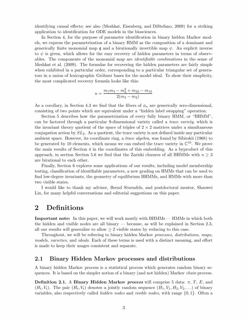
In Section 4, for the purpose of parameter identification in binary hidden Markov mod-els, we express the parametrization of a binary HMM as the composition of a dominant andgenerically finite monomial map q and a birationally invertible map ψ. An explicit inverseto ψ is given, which allows for the easy recovery of hidden parameters in terms of observ-ables. The components of the monomial map are identifiable combinations in the sense ofMeshkat et al. (2009). The formulae for recovering the hidden parameters are fairly simplewhen exhibited in a particular order, corresponding to a particular triangular set of genera-tors in a union of lexicographic Grobner bases for the model ideal. To show their simplicity,the most complicated recovery formula looks like this:

u =m1m3 −m2

2 +m23 −m12

2(m3 −m2)

As a corollary, in Section 4.3 we find that the fibers of φn are generically zero-dimensional,consisting of two points which are equivalent under a “hidden label swapping” operation.

Section 5 describes how the parametrization of every fully binary HMM, or “BHMM”,can be factored through a particular 9-dimensional variety called a trace variety, which isthe invariant theory quotient of the space of triples of 2 × 2 matrices under a simultaneousconjugation action by SL2. As a quotient, the trace variety is not defined inside any particularambient space. However, its coordinate ring, a trace algebra, was found by Sibirskii (1968) tobe generated by 10 elements, which means we can embed the trace variety in C10. We provethe main results of Section 4 in the coordinates of this embedding. As a byproduct of thisapproach, in section Section 5.6 we find that the Zariski closures of all BHMMs with n ≥ 3are birational to each other.

Finally, Section 6 explores some applications of our results, including model membershiptesting, classification of identifiable parameters, a new grading on HMMs that can be used tofind low-degree invariants, the geometry of equilibrium BHMMs, and HMMs with more thantwo visible states.

I would like to thank my advisor, Bernd Sturmfels, and postdoctoral mentor, ShaoweiLin, for many helpful conversations and editorial suggestions on this paper.

2 Definitions

Important note: In this paper, we will work mostly with BHMMs — HMMs in which boththe hidden and visible nodes are all binary — because, as will be explained in Section 2.3,all our results will generalize to allow ≥ 2 visible states by reducing to this case.

Throughout, we will be referring to binary hidden Markov processes, distributions, maps,models, varieties, and ideals. Each of these terms is used with a distinct meaning, and effortis made to keep their usages consistent and separate.

2.1 Binary Hidden Markov processes and distributions

A binary hidden Markov process is a statistical process which generates random binary se-quences. It is based on the simpler notion of a binary (and not hidden) Markov chain process.

Definition 2.1. A Binary Hidden Markov process will comprise 5 data: π, T , E, and(Ht, Vt). The pair (Ht, Vt) denotes a jointly random sequence (H1, V1,H2, V2, . . .) of binaryvariables, also respectively called hidden nodes and visible nodes, with range 0, 1. Often a

3

bound n on the (discrete) time index t is also given. The joint distribution of the nodes isspecified by the following:

• A row vector π = (π0, π1), called the initial distribution, which specifies a probabilitydistribution on the first hidden node H1 by Pr(H1 = i) = πi;

• Amatrix T =

[T00 T01T10 T11

], called the transition matrix, which specifies conditional “tran-

sition” probabilities by the formula Pr(Ht = j |Ht−1 = i) = Tij, read as the probabilityof “transitioning from hidden state i to hidden state j”.2

• AmatrixE =

[E00 E01

E10 E11

], called the emission matrix, which specifies conditional “emis-

sion” probabilities by the formula Pr(Vt = j |Ht = i) = Eij , read as the probabilitythat “hidden state i emits the visible state j”.

To be precise, the parameter vector θ = (π, T,E) determines a probability distributionon the set of sequences of pairs ((H1, V1) . . . (Hn, Vn)) ∈ (0, 12)n, or if no bound n isspecified, a compatible sequence of such distributions as n grows. In applications, only thejoint distribution on the visible nodes (V1, . . . , Vn) ∈ 0, 1n is observed, and is called theobserved distribution. This distribution is given by marginalizing (summing) over the possiblehidden states of a BHM process:

Pr(V = v | θ = (π, T,E)) =∑

h∈0,1n

Pr(h, v|π, T,E) =∑

h∈0,1n

Pr(h |π, T ) Pr(v |h,E)

=∑

h∈0,1n

πh1Eh1,v1

n∏

i=2

Thi−1hiEhi,vi (1)

Definition 2.2. A Binary Hidden Markov distribution is a probability distribution onsequences v ∈ 0, 1n of jointly random binary variables (V1, . . . , Vn) which arises as theobserved distribution of some BHM process according to (1).

As we will see in Section 4.1, different processes (π, T,E,Ht, Vt) can give rise to the sameobserved distribution on the Vt, for example by permuting the labels of the hidden variables,or by other relations among the parameters.

Those already familiar with Markov models in some form may note that:

• The data (π, T,Ht) alone specify what is ordinarily called a binary Markov chain processon the nodes Ht. In the applications we have in mind, these nodes are unobservedvariables.

• The matrices T and E are assumed to be stationary, meaning that they are not allowedto vary with the “time index” t of (Ht, Vt).

• The distribution π is not assumed to be at equilibrium, i.e. we do not assume thatπT = π. This allows for more diverse applications.

N.B. 2.3. The term “stationary” is sometimes also used for a process that is at equilibrium;we will reserve the term “stationary” for the constancy of matrices T ,E over time.

2(Schonhuth, 2011) uses T for different matrices, which I will later denote by P .

4

2.2 Binary Hidden Markov maps, models, varieties, and ideals

Statistical processes come in families defined by allowing their parameters to vary, and inshort, the set of probability distributions that can arise from the processes in a given familyis called a statistical model. The Zariski closure of such a model in an appropriate complexspace is an algebraic variety, and the geometry of this variety carries information about thepurely algebraic properties of the model.

In a binary hidden Markov process, π, T , and E must be stochastic matrices, i.e. each oftheir rows must consist of non-negative reals which sum to 1, since these rows are probabilitydistributions. We denote by Θst the set of such triples (π, T,E), which is isometric to the5-dimensional cube (∆1)

5. We call Θst the space of stochastic parameters. It is helpful to alsoconsider the larger space of triples (π, T,E) where the matrices can have arbitrary complexentries with row sums of 1. We write ΘC for this larger space, which is equal to complexZariski closure of Θst, and call is the space of complex parameters.

We will not simply replace Θst by ΘC for convenience, as has sometimes been done inalgebraic phylogenetics. For the ring of polynomial functions on these spaces, we write

C[θ] := C[πj, Tij , Eij ]

/(1 =

∑

j

πj =∑

j

Tij =∑

j

Eij for i = 0, 1)

so as to make the identification Θst ⊆ ΘC = SpecC[θ]. Here Spec denotes the spectrumof a ring; see (Cox, Little, and O’Shea, 2007) for this and other fundamentals of algebraicgeometry.

Now we a fix a length |v| = n for our binary sequences v, and write

Rp,n := C[pv | v ∈ 0, 1n] C2np := Spec(Rp,n)

Rp,n := Rp,n/(1−

∑

|v|=n

pv) C2n−1p := Spec(Rp,n)

P2n−1p := Proj(Rp,n)

We will often have occasion to consider the natural inclusions,

ιn : C2n−1p → C2n

p ιn : C2n−1p → P2n−1

p

Convention 2.4. Complex spaces such as C2n will usually be decorated with a subscript toindicate the intended coordinates to be used on that space, like the p in C2n

p above. Likewise,a ring will usually be denoted by R with some subscripts to indicate its generators.

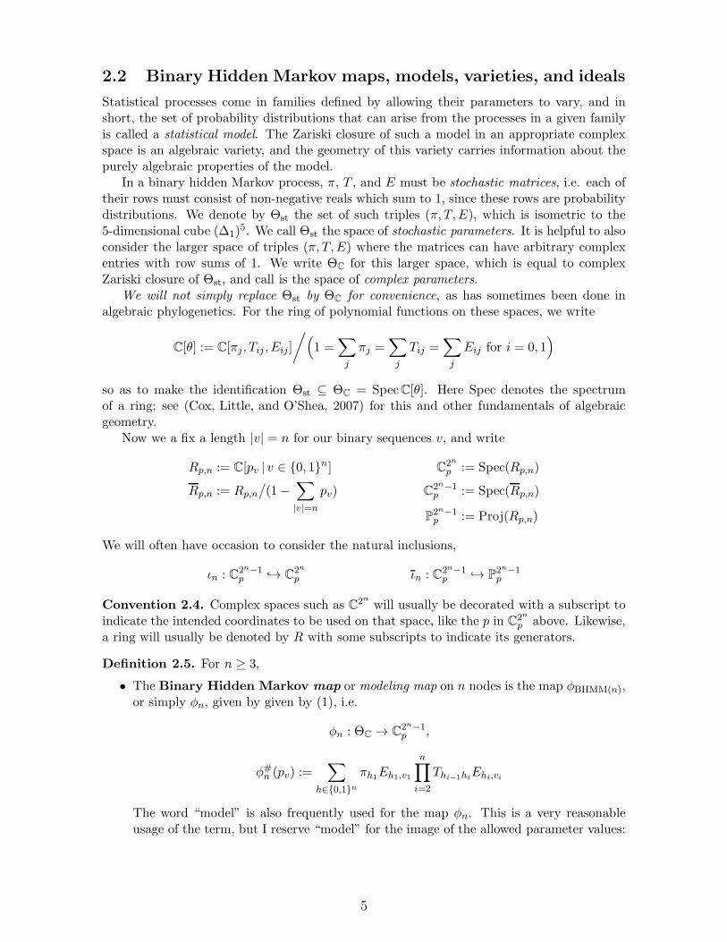
Definition 2.5. For n ≥ 3,

• The Binary Hidden Markov map or modeling map on n nodes is the map φBHMM(n),or simply φn, given by given by (1), i.e.

φn : ΘC → C2n−1p ,

φ#n (pv) :=∑

h∈0,1n

πh1Eh1,v1

n∏

i=2

Thi−1hiEhi,vi

The word “model” is also frequently used for the map φn. This is a very reasonableusage of the term, but I reserve “model” for the image of the allowed parameter values:

5

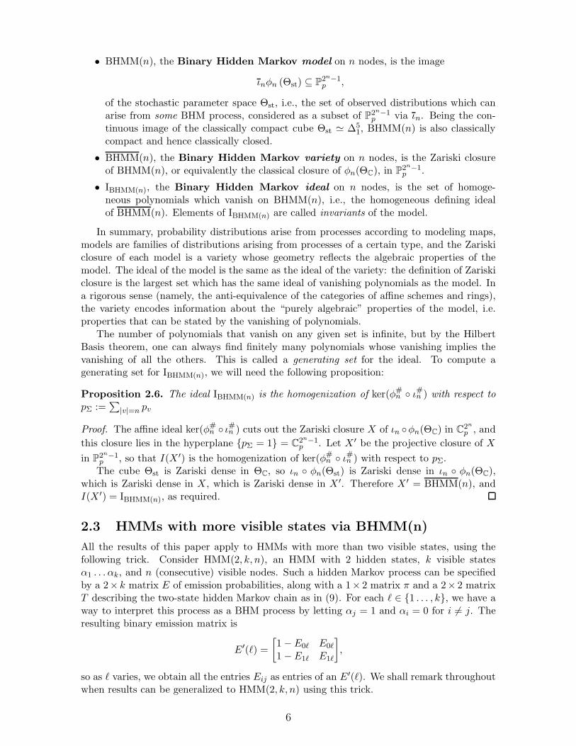
• BHMM(n), the Binary Hidden Markov model on n nodes, is the image

ιnφn (Θst) ⊆ P2n−1p ,

of the stochastic parameter space Θst, i.e., the set of observed distributions which canarise from some BHM process, considered as a subset of P2n−1

p via ιn. Being the con-tinuous image of the classically compact cube Θst ≃ ∆5

1, BHMM(n) is also classicallycompact and hence classically closed.

• BHMM(n), the Binary Hidden Markov variety on n nodes, is the Zariski closureof BHMM(n), or equivalently the classical closure of φn(ΘC), in P2n−1

p .

• IBHMM(n), the Binary Hidden Markov ideal on n nodes, is the set of homoge-neous polynomials which vanish on BHMM(n), i.e., the homogeneous defining idealof BHMM(n). Elements of IBHMM(n) are called invariants of the model.

In summary, probability distributions arise from processes according to modeling maps,models are families of distributions arising from processes of a certain type, and the Zariskiclosure of each model is a variety whose geometry reflects the algebraic properties of themodel. The ideal of the model is the same as the ideal of the variety: the definition of Zariskiclosure is the largest set which has the same ideal of vanishing polynomials as the model. Ina rigorous sense (namely, the anti-equivalence of the categories of affine schemes and rings),the variety encodes information about the “purely algebraic” properties of the model, i.e.properties that can be stated by the vanishing of polynomials.

The number of polynomials that vanish on any given set is infinite, but by the HilbertBasis theorem, one can always find finitely many polynomials whose vanishing implies thevanishing of all the others. This is called a generating set for the ideal. To compute agenerating set for IBHMM(n), we will need the following proposition:

Proposition 2.6. The ideal IBHMM(n) is the homogenization of ker(φ#n ι#n ) with respect topΣ :=

∑|v|=n pv

Proof. The affine ideal ker(φ#n ι#n ) cuts out the Zariski closure X of ιn φn(ΘC) in C2np , and

this closure lies in the hyperplane pΣ = 1 = C2n−1p . Let X ′ be the projective closure of X

in P2n−1p , so that I(X ′) is the homogenization of ker(φ#n ι#n ) with respect to pΣ.The cube Θst is Zariski dense in ΘC, so ιn φn(Θst) is Zariski dense in ιn φn(ΘC),

which is Zariski dense in X, which is Zariski dense in X ′. Therefore X ′ = BHMM(n), andI(X ′) = IBHMM(n), as required.

2.3 HMMs with more visible states via BHMM(n)

All the results of this paper apply to HMMs with more than two visible states, using thefollowing trick. Consider HMM(2, k, n), an HMM with 2 hidden states, k visible statesα1 . . . αk, and n (consecutive) visible nodes. Such a hidden Markov process can be specifiedby a 2× k matrix E of emission probabilities, along with a 1× 2 matrix π and a 2× 2 matrixT describing the two-state hidden Markov chain as in (9). For each ℓ ∈ 1 . . . , k, we have away to interpret this process as a BHM process by letting αj = 1 and αi = 0 for i 6= j. Theresulting binary emission matrix is

E′(ℓ) =

[1−E0ℓ E0ℓ

1−E1ℓ E1ℓ

],

so as ℓ varies, we obtain all the entries Eij as entries of an E′(ℓ). We shall remark throughout

when results can be generalized to HMM(2, k, n) using this trick.

6

3 Defining equations of BHMM(3) and BHMM(4)

Theorem 3.1. The homogeneous ideal IBHMM(4) of the binary hidden Markov variety BHMM(4)is minimally generated by 21 homogeneous quadrics and 29 homogeneous cubics.

Since Schonhuth (2011) found numerically that his Hankel minors did not cut out BHMM(4)even set-theoretically, these equations are genuinely new invariants of the model. Moreover,they are not only applicable to BHMM(4), because a BHM process of length n > 4 canbe marginalized to any 4 consecutive hidden-visible node pairs to obtain a BHM process oflength 4. Thus, we have n−3 linear maps from BHMM(n) to BHMM(4), each of which allowsus to write 21 quadrics and 29 cubics which vanish on BHMM(n). Finally, using Section 2.3,we can even obtain invariants of HMM(2, k, n) via the k different reductions to BHMM(n).

Our fastest derivation of Theorem 3.1 in Macaulay2 (Grayson and Stillman, Grayson and Stillman)uses the birational parametrization of Section 4, but in only a single step, so we defer thelengthier discussion of the parametrization until then. Modulo this dependency, the proof isdescribed in Section 3.3, using moment coordinates (Section 3.1) and cumulant coordinates(Section 3.2).

In probability coordinates, the generators found for IBHMM(4) had the following sizes:

• Quadrics g2,1, . . . , g2,21: respectively 8, 8, 12, 14, 16, 21, 24, 24, 26, 26, 28, 32, 32, 41,42, 43, 43, 44, 45, 72, 72 probability terms.

• Cubics g3,1, . . . , g3,29: respectively 32, 43, 44, 44, 44, 52, 52, 56, 56, 61, 69, 71, 74, 76, 78,81, 99, 104, 109, 119, 128, 132, 148, 157, 176, 207, 224, 236, 429 probability terms.

As a motivation for introducing moment coordinates, we note here that these generators haveconsiderably fewer terms when written in terms of moments:

• Quadrics g2,1, . . . , g2,21: respectively 4, 4, 4, 4, 6, 6, 6, 6, 6, 6, 6, 6, 8, 8, 8, 8, 8, 10, 10, 10, 17moment terms.

• Cubics g3,1, . . . , g3,29: respectively 5, 6, 6, 6, 6, 6, 6, 6, 6, 6, 6, 8, 8, 8, 8, 10, 10, 10, 10, 10, 12,12, 13, 14, 16, 18, 21, 27, 35 moment terms.

To give a sense of how these polynomials look in moment coordinates, the shortest quadricand cubic are

• g2,1 = m23m13 −m2m134 −m13m12 +m1m124, and

• g3,1 = m312 − 2m1m12m123 +m∅m

2123 +m2

1m1234 −m∅m12m1234.

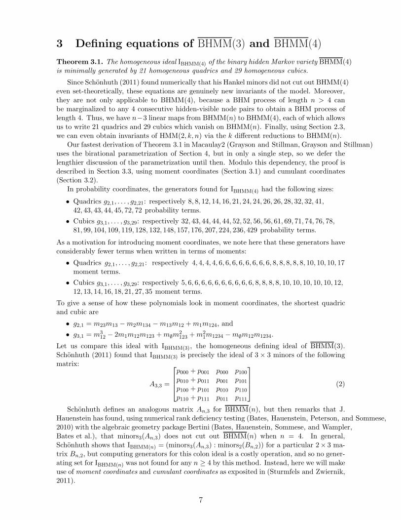
Let us compare this ideal with IBHMM(3), the homogeneous defining ideal of BHMM(3).Schonhuth (2011) found that IBHMM(3) is precisely the ideal of 3× 3 minors of the followingmatrix:

A3,3 =

p000 + p001 p000 p100p010 + p011 p001 p101p100 + p101 p010 p110p110 + p111 p011 p111

(2)

Schonhuth defines an analogous matrix An,3 for BHMM(n), but then remarks that J.Hauenstein has found, using numerical rank deficiency testing (Bates, Hauenstein, Peterson, and Sommese,2010) with the algebraic geometry package Bertini (Bates, Hauenstein, Sommese, and Wampler,Bates et al.), that minors3(An,3) does not cut out BHMM(n) when n = 4. In general,Schonhuth shows that IBHMM(n) = (minors3(An,3) : minors2(Bn,2)) for a particular 2× 3 ma-trix Bn,2, but computing generators for this colon ideal is a costly operation, and so no gener-ating set for IBHMM(n) was not found for any n ≥ 4 by this method. Instead, here we will makeuse of moment coordinates and cumulant coordinates as exposited in (Sturmfels and Zwiernik,2011).

7

3.1 Moment coordinates

Moments are particular linear expressions in probabilities. They can be derived from amoment generating function as in (Sturmfels and Zwiernik, 2011), but in our case, momentscan be expressed simply by the following rule: we order 0, 1n by strict dominance, i.e.v ≥ wiff vi ≥ wi for all i, and then

mv :=∑

w≥v

pw ∈ Rp,n (3)

Since all our variables are binary, with the usual algebraic statistical convention that a “+”subscript denotes an index to be summed over, we can view the conversion from momentsto probabilities as “replacing zeros by + signs”. For example, m10010 = p1++1+. The ringelements mv ∈ Rp,n provide alternative linear coordinates on P2n−1

p in which it turns out thatsome previously intractable BHM computations are simplified and become feasible.

For a more compact notation, a binary string v of length n is the indicator function ofa unique subset I of [n] = 1, . . . , n, so we also write mI to represent mv. For example,m0000 = m∅, m1000 = m1, and m0101 = m24. From (3) we can see that mI actually representsa marginal probability: mI = Pr(Vi = 1 for all i ∈ I). Thus, in the context of BHMMs , noconfusion results if we write mI without specifying the value of n. To be precise, if I ⊆ [n]and I ′ denotes I considered as a subset of [n′] for some n′ > n, then

φ#n (mI) = φ#n′(mI′) (4)

This can be seen in many ways, for example using the Baum formula for moments (Proposition 5.1)as explained in Section 5.3.

Just as for probabilities, for moments we define rings and spaces

Rm,n := C[mI | I ⊆ [n]] C2n

m := Spec(Rm,n)

Rm,n := Rm,n/〈1−m∅〉 C2n−1

m := Spec(Rm,n) (5)

P2n−1m := Proj(Rm,n),

To avoid having notation for too many ring isomorphisms, we adopt:

Convention 3.2. Using (3), we will usually treat mI as a literal element of Rp,n, thuscreating literal identifications

Rm,n = Rp,n, Rm,n = Rp,n, C2nm = C2n

p , P2n−1m = P2n−1

p , and C2n−1m = C2n−1

p . (6)

Note that, for example, we obtain natural ring inclusions

Rm,n ⊆ Rm,n′

whenever n < n′, which respect the BHM maps φn because of (4).As a first application of moment coordinates, we have

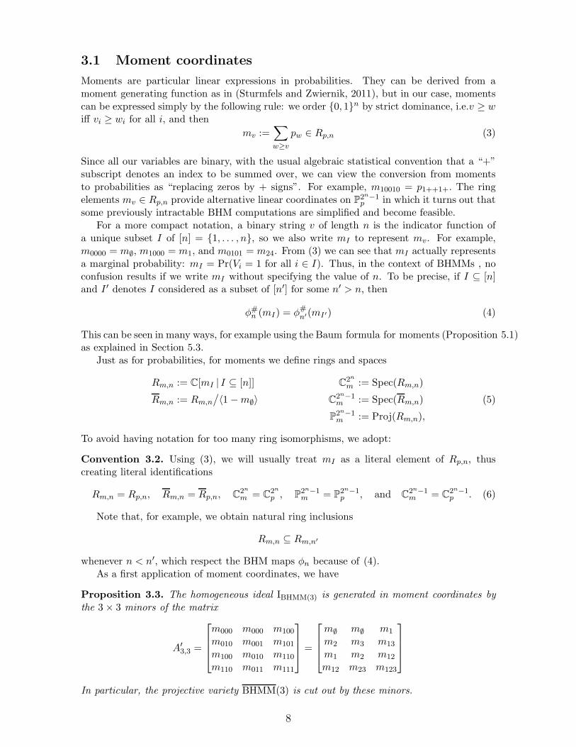
Proposition 3.3. The homogeneous ideal IBHMM(3) is generated in moment coordinates bythe 3× 3 minors of the matrix

A′3,3 =

m000 m000 m100

m010 m001 m101

m100 m010 m110

m110 m011 m111

=

m∅ m∅ m1

m2 m3 m13

m1 m2 m12

m12 m23 m123

In particular, the projective variety BHMM(3) is cut out by these minors.

8

Proof. Observe that Schonhuth’s matrix A3,3 in (2) is equivalent under elementary row/columnoperations to A′

3,3, so minors3A′3,3 = minors3A3,3 = IBHMM(3).

Proposition 3.4. The ideal IBHMM(n) is the homogenization of ker(φ#n ) with respect to m∅.

Proof. From Proposition 2.6 we know that IBHMM(n) is the homogenization of ker(φ#n ι#n )with respect to m∅ =

∑|v|=n pv. From (5), we can identify Rm,4 with the polynomial subring

of Rm,4 obtained by omitting m∅, so that ker(φ#4 ι#4 ) = ker(φ#4 ) + 〈1 − m∅〉. Since the

additional generator 1 − m∅ homogenizes to 0, ker(φ#4 ) has the same homogenization as

ker(φ#4 ι#4 ), hence the result.

3.2 Cumulant coordinates

Cumulants are non-linear expressions in moments or probabilities which seem to allow evenfaster computations with binary hidden Markov models. Let

Rk,n := C[kI | I ⊆ [n]]

Rk,n := Rk,n/〈k∅〉

C2n−1k := Spec(Rk,n)

where, as with moments, we may freely alternate between writing kv and writing kI , whereI is the set of positions where 1 occurs in v. For building generating functions, let x1, . . . , xnbe indeterminates, and write xv = xI for xv11 · · · xvnn =

∏i∈I xi. Let J be the ideal generated

by all the squares x2i . Following (Sturmfels and Zwiernik, 2011), we define the moment andcumulant generating functions, respectively, as

fm(x) :=∑

I⊆[n]

mIxI ∈ Rm,n[x]/J fk(x) :=

∑

I⊆[n]

kIxI ∈ Rk,n[x]/J

We now define changes of coordinates

κn : C2n−1m → C2n−1

k κ−1n : C2n−1

k → C2n−1m

by the formulae

κ#n (fk) = log(fm) =(fm − 1)

1+ · · · + (−1)n+1 (fm − 1)n

n(7)

κ−#n (fm) = exp(fk) = 1 +

(fk)

1+ · · ·+ (fk)

n

n!

That is, we let κ#n (kI) be the coefficient of xI in the Taylor expansion of log fm about 1, and

let κ−#n (mI) be the coefficient of xI in the Taylor expansion of exp fk about 0. Note that in

the relevant coordinate rings Rm,n and Rk,n, m∅ = 1 and k∅ = 0. This is why we only needto compute the first n terms of each Talyor expansion: the higher terms all vanish modulothe ideal J .

Proposition 3.5. The expressions κ#n (kI) and κ−#n (mI), i.e. writing of cumulants in terms

of moments and conversely, do not depend on n.

Proof. In (Sturmfels and Zwiernik, 2011), these formulae are re-expressed using Mobius func-tions, which do not depend on the generating function description above, and in particulardo not depend on n.

9

3.3 Deriving IBHMM(4) in Macaulay2

This section describes the proof of Theorem 3.1 using Macaulay2. These computations werecarried out on a Toshiba Satellite P500 laptop running Ubuntu 10.04, with an Intel Core i7Q740 .73 GHz CPU and 8gb of RAM. In light of Proposition 3.4, we will aim to computeker(φ#4 ι#4 ), which can be understood geometrically as the (non-homogeneous) ideal of thestandard affine patch of BHMM(4) where m∅ =

∑|v|=4 pv = 1. To reduce the number of

variables, as in Proposition 3.4 we continue to make the identification

Rm,4 = C[mI |∅ 6= I ⊆ [4]] ⊆ Rm,4

We begin by providing Macaulay2 with the map φ#4 : Rm,4 → C[θ] in moment coordinates(Section 3.1), because probability coordinates result in longer, higher degree expressions. This

can be done by composing the expression of φ#n (pv) in Definition 2.5 with the expression ofmv = mI in (3), or alternatively using the Baum formula for moments (Proposition 5.1),which involves many fewer arithmetic operations.

Macaulay2 runs out of memory (8gb) trying to compute ker(φ#4 ), and as expected, thismemory runs out even sooner in probability coordinates, so we use cumulant coordinatesinstead (Section 3.2). We input

κ#4 : Rk,4 → Rm,4

using coefficient extraction from (7), and compute the composition φ#4 κ#4 . Then, it ispossible to compute

Ik,4 := ker(φ#4 κ#4 )which takes around 1.5 hours. Alternatively, we can compute Ik,4 using the birationalparameterization ψ4 of Section 4 in place of φ4, which takes less than 1 second and yields100 generators for Ik,4.

Subsequent computations run out of memory with this set of 100 generators, so we musttake some steps to simplify it. Macaulay2’s trim command reduces the number of generatorsof Ik,4 to 46 in under 1 second. We then order these 46 generators lexicographically, firstby degree and then by number of terms, and eliminate redundant generators in reverse order,which takes 19 seconds. The result is an inclusion-minimal, non-homogeneous generatingset for Ik,4 with 35 generators: 24 quadrics and 11 cubics.

Now we compute Im,4 := κ#(Ik,4) = κ#(ker(φ#4 κ#4 )) = ker(φ#4 ), i.e., we push forward

the 35 generators for Ik,4 under the non-linear ring isomorphism κ#4 to obtain 35 generators

for Im,4 = ker(φ#4 ): 2 quadrics, 7 cubics, 16 quartics, 5 quintics, and 5 sextics. In under 1

second, Macaulay2’s trim command computes a new set of 39 generators for Im,4 with lowerdegrees: 21 quadrics, 14 cubics, and 4 quartics, which turns out to save around 1 hour ofcomputing time in what follows. These generators have many terms each, and eliminatingredundant generators as in the previous paragraph turns out to be too slow to be worth ithere, taking more than 2 hours, so we omit this step.

Finally, we apply Proposition 3.4 to compute IBHMM(4) as the homogenization of Im,4 withrespect to m∅. In Macaulay2, this is achieved by homogenizing the 39 generators for Im,4 withrespect to m∅ and then saturating the ideal they generate with respect to m∅. This saturationoperation takes about 29 minutes, and yields a minimal generating set of 50 polynomials:21 quadrics and 29 cubics. Since probabilities are linear in moments, their degrees are thesame in probability coordinates. Moreover, since these are homogeneous generators for ahomogeneous ideal, they are minimal in a very strong sense:

Corollary 3.6. Any inclusion-minimal homogeneous generating set for IBHMM(4) in proba-bility or moment coordinates must contain exactly 21 quadrics and 29 cubics.

10

We still do not know a generating set for IBHMM(5). Macaulay2 runs out of memory (8gb)attempting to compute Ik,5, even using the birational parametrization of Section 4. Theauthor has also attempted this computation using the tree cumulants of Smith and Zwiernik(2010) in place of cumulants, but again Macaulay2 runs out of memory trying to compute thefirst kernel. Presumably the subsequent saturation step would be even more computationallydifficult.

4 Birational parametrization of BHMMs

Theorem 4.1 (Birational Parameter Theorem). There is a generically two-to-one, dominantmorphism ΘC → C5 such that, for each n ≥ 3, the binary hidden Markov map φn factorsuniquely as follows, and each ψn : C5 → BHMM(n) has a birational inverse map ρn:

C5 C2n−1p

ψnΘC

φn

C5 BHMM(n)

ψn

ρn

In particular, BHMM(n) is always a rational projective variety of dimension 5, i.e., bira-tionally equivalent to P5.

Using the reduction of Section 2.3, the same is true if we allow k > 2 visible states inthe model and replace 5 by 3 + k. This theorem will be proven in Section 5.6 using tracealgebras and the Baum formula for moments. In the course of this section and Section 5we will exhibit formulae for ψn and their inverses ρn. The inverse map ρ3 has a number ofpractical uses, to be explored in Section 6.

Our first step toward Theorem 4.1 is to re-parametrize ΘC.

4.1 A linear reparametrization of ΘC

Since the hidden variables Ht are never observed, there is no change in the final expression ofpv in Definition 2.5 if we swap the labels 0, 1 of all the Ht simultaneously. This swappingis equivalent to an action of the elementary permutation matrix σ = ( 0 1

1 0 ):

sw : ΘC → ΘC

θ = (π, T,E) 7→ (πσ, σ−1Tσ, σ−1E) (8)

(In our case σ−1 = σ, but the form above generalizes to permutations of larger hiddenalphabets.) Hence we have that Pr(v |π, T,E) = Pr(v | sw(π, T,E)), i.e. φn = φn sw.

We will make essential use of a linear parametrization of ΘC in which sw has a simple form.Our new parameters will be η0 := (a0, b, c0, u, v0), with subscript 0’s to be explained shortly.Although we have already used the letter v at times to represent visible binary strings, wehope that the context will be clear enough to avoid confusion between these usages. We let

π =1

2

[1− a0, 1 + a0

]

T =1

2

[1 + b− c0, 1− b+ c01− b− c0, 1 + b+ c0

]E =

[1− u+ v0, u− v01− u− v0, u+ v0

] (9)

(The rightmost column of E is made intentionally homogeneous in the new parameters.) Wecan linearly solve for η0 in terms of θ by a0 = π1− π0 etc., so in fact (a0, b, c0, u, v0) generatethe parameter ring C[θ]. In these coordinates, sw acts by

a0 7→ −a0, b 7→ b, c0 7→ −c0, u 7→ u, v0 7→ −v0

11

In other words, swapping the signs of the subscripted variables a0, c0, v0 has the same effectas acting on the matrices π, T,E by σ as in (8), i.e., relabeling the hidden alphabet.

4.2 Introducing the birational parameters

Since φn sw = φn, by classical invariant theory the ring map φ#n : Rp,n → C[θ] must land

in the subring of invariants C[θ]sw = C[b, u, a20, c20, v

20 , a0c0, a0v0, c0v0]. However, φ

#n in fact

factors through a smaller subring, conveniently generated by 5 elements:

Lemma 4.2 (Parameter Subring Lemma). For all n ≥ 3, the ring map φ#n lands in thesubring

C[η] := C[a, b, c, u, v]

of C[θ], where a = a0v0, c = c0v0, v = v20.

The proof of this key lemma will be given in Section 5.5 after introducing trace algebras.To interpret its geometric consequences, write q

# for the subring inclusion

q# : C[η] → C[θ]

a 7→ a0v0, b 7→ b, c 7→ c0v0, u 7→ u, v 7→ v20 ,

write ψ#n : Rp,n → C[η] for the factorization of φ#n through q

#, and write Θ′C := SpecC[η],

so Θ′C ≃ C5. The result:

Corollary 4.3. The following diagram of dominant maps commutes

Θ′C BHMM(n)

ψnΘC

φn

q

and q is generically two-to-one.

This corollary in particular implies the first part of the Birational Parameter Theorem(4.1), by taking q : ΘC → Θ′

C ≃ C5 as the generically 2 : 1 map.

Remark 4.4. The map q is only dominant, and not surjective; for example, it misses thepoint (1, 0, 0, 0, 0).

Corollary 4.5. For all n ≥ 3, BHMM(n) = image(ιnψn).

Proof. Since q is dominant, image(ιnψn) = image(ιnψnq) = image(ιnφn) =: BHMM(n).

The unique factorization map ψ#n can be computed directly in Macaulay2 for small n.

The expressions in moment coordinates are simpler than in probabilities, so we present thesein the following proposition.

12

Proposition 4.6. The map ψ#3 is given in moment coordinates by

m∅ = m000 7→ 1

m1 = m100 7→ a+ u

m2 = m010 7→ ab+ c+ u

m3 = m001 7→ ab2 + bc+ c+ u

m12 = m110 7→ abu+ ac+ au+ cu+ u2 + bv

m13 = m101 7→ ab2u+ abc+ bcu+ b2v + ac+ au+ cu+ u2

m23 = m011 7→ ab2u+ abc+ abu+ bcu+ c2 + 2cu+ u2 + bv

m123 = m111 7→ ab2u2 + 2abcu+ abu2 + bcu2 + b2uv + ac2 + 2acu

+ c2u+ au2 + 2cu2 + u3 + abv + bcv + 2buv

We will eventually prove the Birational Parameter Theorem (4.1) by marginalization tothe case n = 3, which we can prove here:

Proposition 4.7. The following triangular set of equations hold on the graph of ψ3, afterclearing denominators, and can thus be used to recover parameters from observed momentswhere the denominators are non-zero:

b =m3 −m2

m2 −m1

u =m1m3 −m2

2 +m23 −m12

2(m3 −m2)

a = m1 − uc = a− ba+m2 −m1

v = a2 − m1m2 −m12

b

(This proposition and the following corollary actually hold for all φn with n ≥ 3, because ofProposition 5.2, and by Section 2.3, these same formulae can be used to recover parametersfor HMM(2, k, n) when k > 2 as well.)

Proof. These equations can be checked with direct substitution by hand from Proposition 4.6.Regarding the derivation, they can be obtained in Macaulay2 by computing two Grobner basesof the elimination ideal I = 〈mv − φ3(mv)|v ∈ 0, 13〉 over the ring C23

m , in Lex monomialorder: once in the ring Rm,3[v, c, a, b, u], and once in Rm,3[v, c, u, b, a]. Each variable occursin the leading term of a some generator in one of these two bases with a simple expressionin moments as its leading coefficient. We solve each such generator (set to 0) for the desiredparameter.

Corollary 4.8. The map ψ3 : C5 → BHMM(3) has a birational inverse ρ3. The map ρ#3 onmoment coordinate functions is given by:

a 7→ m22 +m3m1 − 2m2m1 −m23 +m12

2(m3 −m2)u 7→ −m

22 +m3m1 +m23 −m12

2(m3 −m2)

b 7→ m3 −m2

m2 −m1v 7→ num(v)

4(m3 −m2)2

c 7→ num(c)

2(m2 −m1)(m3 −m2), where

13

num(c) =−m1m22 +m2

1m3 +m22m3 −m1m

23 −m1m12

+ 2m2m12 −m3m12 +m1m23 − 2m2m23 +m3m23, and

num(v) = m42 − 2m1m

22m3 +m2

1m23 − 2m2

2m12 − 2m1m3m12 + 4m2m3m12

+ 4m1m2m23 − 2m22m23 − 2m1m3m23 +m2

12 − 2m12m23 +m223.

Proof. This can be derived by substituting the solutions for u, a, and b in the previouspropositions into the subsequent solutions for a, c, and v. Alternatively, it can be checked bydirect substitution in Macaulay2, i.e., one computes that ψ#

3 ρ#(θ) = θ for each birationalparameter θ ∈ a, b, c, u, v.

The expressions in Corollary 4.8 are considerably simpler in moment coordinates than inprobabilities. Comparing the number of terms, the numerators for a, b, c, u, v respectivelyhave sizes 5, 2, 10, 4, and 12 in moment coordinates, versus sizes 22, 4, 56, 22, and 190 inprobability coordinates. This explains in part why Macaulay2’s Grobner basis computationsexecute in moment coordinates with much less time and memory.

4.3 Statistical interpretation of the birational inverse ρ3

It turns out that the factors appearing in the denominators of Corollary 4.8 defining ρ3 havesimple factorizations in terms of the rational and birational parameters:

• m3 −m2 appears in the denominator of all ρ3(θ) except ρ3(b), and

m3 −m2ψ37→ (b)(ab− a+ c)

q7→ (b)(v0)(a0b− a0 + c0)

• m2 −m1 appears in the denominator of ρ3(b) and ρ3(c), and

m2 −m1ψ37→ ab− a+ c

q7→ (v0)(a0b− a0 + c0)

Let us pause to reflect on the meaning of these factors.

• The factor v0 occurs in det(E) = 2v0, hence v = v20 = 0 iff the hidden Markov chainhas “no effect” on the observed variables. The image locus φ3(v0 = 0) can thusbe modeled by a sequence of IID coin flips with distribution E0 = E1 = (1 − u, u),so the BHMM is an unlikely model choice. This is a one-dimensional submodel,parametrizable by u ∈ [0, 1], with a regular (everywhere-defined) inverse given simplyby u = m1. Denote this model by BIID(n).

• The factor b occurs in det(T ) = b, hence b = 0 iff each hidden node has “no effect” onthe subsequent hidden nodes. In this case, the observed process can be modeled as asequence of independent coin flips, the first flip having distribution (1 − α,α) := πEand subsequent flips being IID having distribution (1 − β, β) := T0E = T1E. Theimage locus φ3(b = 0) is hence a two-dimensional submodel, parametrizable by(α, β) ∈ [0, 1]2, with a regular inverse given by α = m1, β = m2. Denote this modelby BINID(n), for “binary independent nearly identically distributed” model, and notethat BINID(n) ⊇ BIID(n) by setting α = β.

• The factor a0b − a0 + c0 occurs in πT − π = 12(−a0b + a0 − c0, a0b − a0 + c0). Hence

a0b−a0+c0 = 0 iff π is a fixed point of T , i.e. the hidden Markov chain is at equilibrium.We may define the Equilibrium Binary Hidden Markov model by restricting φn to thelocus a0b − a0 + c0 = 0), which turns out to yield a four-dimensional submodel

for each n ≥ 3. Denote this submodel by EBHMM(n).

14

It can be easily shown, with the same methods used here for BHMM(n), that EBHMM(n)itself has a birational parametrization by (a0v0, b, u, v

20) = (a, b, u, v), where a0, b ∈ [−1, 1],

c0 := a0(1−b) ∈ [|b|−1, 1−|b|], v0 ∈ [0, 1], and u ∈ [|v0|, 1−|v0|], with an inverse parametriza-tion given by

b =m2

1 −m13

m21 −m12

u =2m1m12 −m1m13 −m123

2(m21 −m13)

a = m1 − u v =a2b−m2

1 +m12

b

The newly occurring denominators here are m21 −m12 = (b)(a2 − v) = (b)(v0)

2(a20 − 1) andm2

1−m13 = (b)2(a2−v) = (b)(v0)2(a20−1). It easy to check that the only points of EBHMM(n)

where these expressions vanish are points that lie in BINID(n). Thus, for n ≥ 3, BHMM(n)can be stratified as a union of three statistically meaningful submodels

BHMM(n) = BINID(n) ← 2 dimensional

∪(EBHMM(n) \ BINID(n)

)← 4 dimensional

∪(BHMM(n) \

(EBHMM(n) ∪ BINID(n)

))← 5 dimensional

each of which has an everywhere-defined inverse parametrization.

4.4 Computational advantages of moments, cumulants, andbirational parameters

Our approach has been to work with moments mv and cumulants kv instead of probabilitiespv, and the birational parameters a, b, c, u, v instead of the matrix entries π1, ti1, ei1. Otherthan the theoretical advantage that the model map is generically injective on the birationalparameter space, significant computation gains in Macaulay2 also result from these choices(see Section 3.3 for laptop specifications):

• Computing kerψ3 = kerφ3, the affine defining ideal of BHMM(3), took less than 1second in Macaulay2 when using the birational parameters, compared to 25 secondswhen using the matrix entries and moments, and 15 minutes when using the matrixentries and probabilities.

• Computing kerψ4 = ker φ4, the affine defining ideal of BHMM(4) took less than 1second in Macaulay2 when using the birational parameters and cumulant coordinates(Sturmfels and Zwiernik, 2011), compared to 1.5 hours when using the matrix entriesand cumulant coordinates, and running out of memory (8gb) when using the matrixentries and probabilities.

5 Parametrizing BHMMs though a trace variety

In this section, we exhibit a parametrization of every BHMM through a particular tracevariety called SpecC2,3, which itself can be embedded in C10. We use these coordinatesto prove the Birational Parameter Theorem (4.1) and the Parameter Subring Lemma (4.2),which were stated without proof.

For this, we will define a map φ∞ through which all the φn factor, and using a version ofthe Baum formula for moments, we factor this map further though SpecC2,3. Then we usea finite set 10 of generators of the ring C2,3 exhibited by (Sibirskii, 1968) to show that theimage of φ∞ lands in the desired subring C[η], and write ψ∞ for the factorization. Finally,

15

by marginalizing to the case n = 3, we obtain a birational inverse for ψn from the map ρ3given in Corollary 4.8.

5.1 Marginalization maps

For each pair of integers n′ ≥ n ≥ 1, the marginalization map µn′

n : C2n′

p → C2np is given by

µn′

n

#(pv) :=

∑

|w|=n′−n

pvw

These restrict to maps µn′

n : C2n′

−1p → C2n−1

p , and define rational maps µn′

n : P2n′

−1p 99K P2n−1

p .

In moment coordinates, these maps are actually coordinate projections: µn′

n

#(mv) = mv0

where 0 denotes a sequence of n′ − n zeros. In fact, using the subset notation for moments

mI , the corresponding ring maps are literal inclusions: µn′

n

#(mI) = mI . In other words,

µn′

n : C2n′

m → C2nm is just the map which forgets those mI where I * [n].

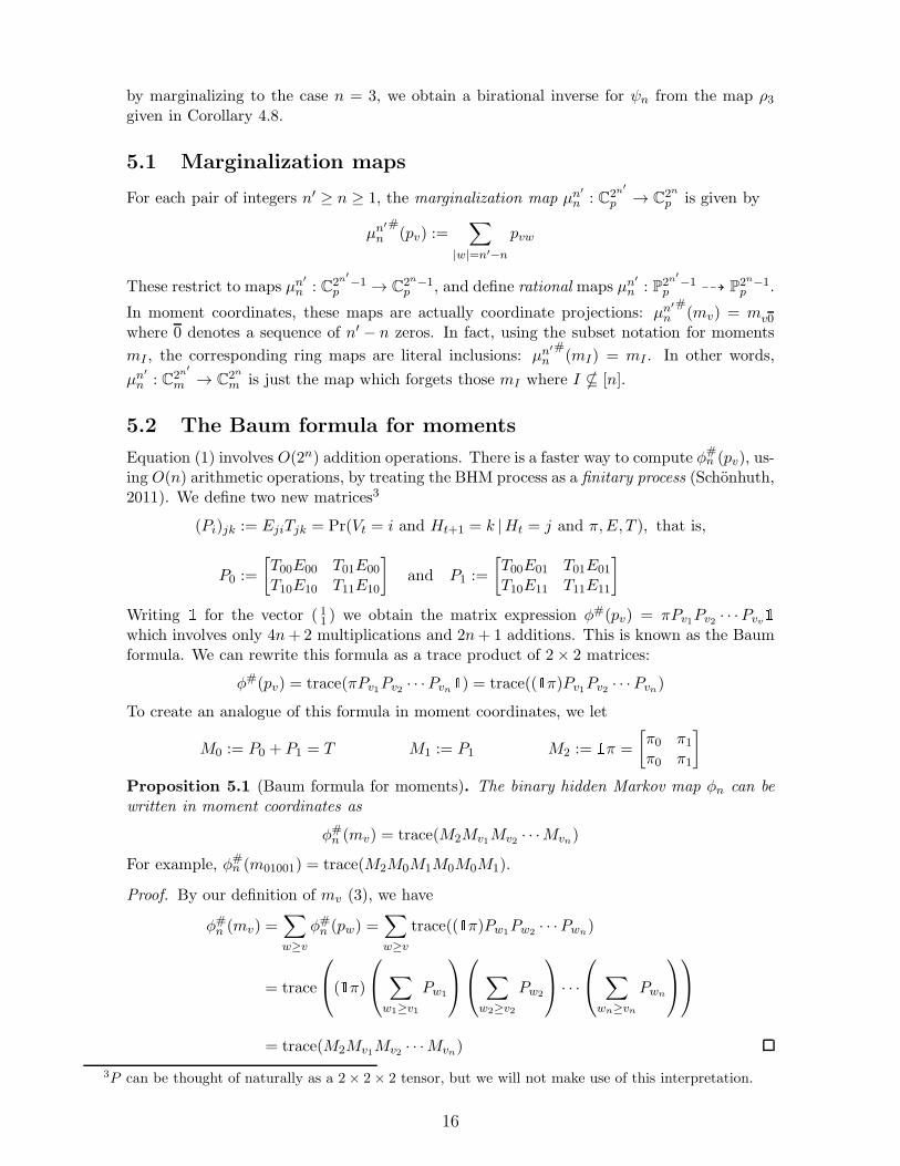
5.2 The Baum formula for moments

Equation (1) involves O(2n) addition operations. There is a faster way to compute φ#n (pv), us-ing O(n) arithmetic operations, by treating the BHM process as a finitary process (Schonhuth,2011). We define two new matrices3

(Pi)jk := EjiTjk = Pr(Vt = i and Ht+1 = k |Ht = j and π,E, T ), that is,

P0 :=

[T00E00 T01E00

T10E10 T11E10

]and P1 :=

[T00E01 T01E01

T10E11 T11E11

]

Writing 1 for the vector ( 11 ) we obtain the matrix expression φ#(pv) = πPv1Pv2 · · ·Pvv1which involves only 4n+2 multiplications and 2n+ 1 additions. This is known as the Baumformula. We can rewrite this formula as a trace product of 2× 2 matrices:

φ#(pv) = trace(πPv1Pv2 · · ·Pvn1) = trace((1π)Pv1Pv2 · · ·Pvn)To create an analogue of this formula in moment coordinates, we let

M0 := P0 + P1 = T M1 := P1 M2 := 1π =

[π0 π1π0 π1

]

Proposition 5.1 (Baum formula for moments). The binary hidden Markov map φn can bewritten in moment coordinates as

φ#n (mv) = trace(M2Mv1Mv2 · · ·Mvn)

For example, φ#n (m01001) = trace(M2M0M1M0M0M1).

Proof. By our definition of mv (3), we have

φ#n (mv) =∑

w≥v

φ#n (pw) =∑

w≥v

trace((1π)Pw1Pw2· · ·Pwn

)

= trace

(1π)

∑

w1≥v1

Pw1

∑

w2≥v2

Pw2

· · ·

∑

wn≥vn

Pwn

= trace(M2Mv1Mv2 · · ·Mvn)

3P can be thought of naturally as a 2× 2× 2 tensor, but we will not make use of this interpretation.

16

5.3 Truncation and φ∞Proposition 5.2. The binary hidden Markov maps φn form a directed system of maps undermarginalization, meaning that, for each n′ ≥ n ≥ 1, the following diagrams commute:

ΘC

C2n−1m

C2n′

−1mφn′

φn

µn′

nC[θ]

Rm,n

Rm,n′φ#n′

φ#n

µn′

n

#

Proof. This can be seen directly from the definition of φn using (1) and of mv in (3). Alter-natively, observe that because M0 = T is stochastic, M0M2 = M2, so for any sequence 0 oflength n′ − n, the Baum formula for moments (Proposition 5.1) implies that

φ#n′(mv0) = φ#n (mv) (10)

Thus, to compute φn for all n, it is only necessary to compute those φ#nmv′ where v′ ends

in 1. Motivated by this observation, let Rm,∞ := C[mv1 | v ∈ 0, 1n for some n ≥ 0] =C[m1,m01,m11,m001,m101,m011, . . .], which in subset index notation is simply

Rm,∞ := C[mI | I ⊆ [n] for some n ≥ 0]

= C[m1,m2,m12,m3,m13,m23, . . .]

Then we define φ∞ : ΘC → SpecRm,∞ and φ#∞ : C[θ]← Rm,∞ by the formula φ#∞(mv10) :=

φ#length(v1)(mv1), i.e.

φ#∞(mI) := φ#size(I)(mI) (11)

Note that by locating the position of the last 1 in a binary sequence v′ 6= 0 . . . 0, we can write v′

in the form v10 for a unique string v (possibly empty if v′ = 1), so this map is well-defined. Bythe same principle, for each n we can also define a “truncation” map τ : SpecRm,∞ → C2n−1

m

by τ#(mv10) := mv1, which, in subset index notation, is a literal ring inclusion:

τ#(mI) := mI (12)

With this definition, φ#n factorizes as φ#n = φ#∞ τ#n . We can summarize this andProposition 5.2 as follows:

Proposition 5.3. For all n′ ≥ n ≥ 1, the following diagrams commute:

ΘC

C2n−1m C2n

′

−1m

SpecRm,∞

φnφn′

φ∞

µn′

nτn′

C[θ]

Rm,n Rm,n′ Rm,∞

φ#nφ#n′

φ#∞

µn′

n

# τ#n′

Remark 5.4. These diagrams exhibit the rings Rm,n and maps φ#n as a directed system

under the inclusion maps µn′

n

#, such that Rm,∞ = colimn→∞Rm,n and φ#∞ = limn→∞ φ#n .

Now, to prove that φn factors through q, we need only show that φ∞ does.

17

5.4 Factoring φ∞ through a trace variety

Let X0,X1,X2 be 2× 2 matrices of indeterminates,

X0 =

[x000 x001x010 x011

]X1 =

[x100 x101x110 x111

]X2 =

[x200 x201x210 x211

]

and following the notation of (Drensky, 2007), Ω2,3 := C[entries of X0,X1,X2] denotes thepolynomial ring on the entries xijk of these three 2 × 2 matrices. The trace algebra C2,3 isdefined as the subring of Ω2,3 generated by the traces of products of these matrices, C2,3 :=C[trace(Xi1Xi2 · · ·Xir) | r ≥ 1] ⊆ Ω2,3 and we refer to SpecC2,3 as a trace variety. We write

ν : SpecΩ2,3 → SpecC2,3 and ν# : C2,3 → Ω2,3

for the natural dominant map and corresponding ring inclusion. To relate these varieties tobinary HMMs , we define two new maps ω# : Ω2,3 → C[θ] and ξ# : Rm,∞ → C2,3 by

ω#(Xi) :=Mi and ξ#(mv1) := trace

((X2

∏

i∈v

Xi

)X1

).

Proposition 5.5 (Baum factorization). The ring map φ#∞ factorizes as φ#∞ = ω# ν# ξ#,i.e., the following diagram commutes:

ΘC

SpecΩ2,3 SpecC2,3

SpecRm,∞

ω

ν

ξ

φ∞

Proof. This is just a restatement of the Baum formula for moments (Proposition 5.1):

ω#(ν#(ξ#(mv1))) = ω# trace

(X2

∏

i∈v1

Xi

)= trace

(M2

∏

i∈v1

Mi

)

= φ#length(v1)

(mv1) = φ#∞(mv1)

5.5 Proving the Parameter Subring Lemma (4.2)

We begin by seeking a factorization of the map ω# ν#. For this we apply the followingcommutative algebra result of Sibirskii on the trace algebras C2,r:

Proposition 5.6 (Sibirskii, 1968). The trace algebra C2,r is generated by the elements

trace(Xi) : 0 ≤ i ≤ rtrace(XiXj) : 0 ≤ i ≤ j ≤ r

trace(XiXjXk) : 0 ≤ i < j < k ≤ r

Corollary 5.7. The algebra C2,3 is generated by the 10 elements

trace(X0), trace(X1), trace(X2),

trace(X20 ), trace(X

21 ), trace(X

22 ), trace(X0X1), trace(X0X2), trace(X1X2),

trace(X0X1X2)

18

Proposition 5.8. The ring map ω# ν# factors through the inclusion

q# : C[η] := C[a, b, c, u, v] → C[θ] := C[a0, b, c0, u, v0],

i.e. we can write ω# ν# = q# r# so that the following diagram commutes:

ΘC

SpecΩ2,3 SpecC2,3

Θ′C

ω

ν

r

q

Proof. We apply ω# to the ten generators of C2,3 given in Corollary 5.7 and check that theyland in C[η]. Explicit, we find that:

trace(M0) = b+ 1 trace(M1) = bu+ c+ u trace(M2) = 1

trace(M20 ) = b2 + 1 trace(M2

1 ) = b2u2 + 2bcu+c2 + 2cu+ u2 + 2bv

trace(M22 ) = 1 trace(M0M1) = b2u+ bc+ c+ u trace(M0M2) = 1

trace(M1M2) = a+ u trace(M0M1M2) = ab+ c+ u

Now, by letting ψ#∞ := r

# ξ# we may factor the ring map φ#∞ as

φ#∞ = ω# ν# ξ# = q# r# ξ# = q

# ψ#∞.

Corollary 5.9. The following diagram commutes:

Θ′CΘC

SpecΩ2,3 SpecC2,3

SpecRm,∞q

r

ψ∞

φ∞

ω

ν

ξ

Proof of the Parameter Subring Lemma (4.2). Proposition 5.3 and Corollary 5.9 together im-ply that the following diagrams commute:

Θ′CΘC SpecRm,∞ C2n−1

m

q ψ∞ τn

φn

C[η]C[θ] Rm,∞ Rm,nq# ψ#

∞ τ#n

φ#n

In particular, the map φ#n factors through C[η], as required.

19

5.6 Proving the Birational Parameter Theorem (4.1)

Recall that Corollary 4.3 implies the first part of the Birational Parameter Theorem (4.1),by taking

q : ΘC −→ Θ′C

as the generically 2 : 1 map. Thus, it remains to show that the maps

ψn : Θ′C −→ BHMM(n)

have birational inverses ρn. The inverse map ρ3 was already exhibited in Corollary 4.8, andwe obtain ρn by marginalization: let

ρn = ρ3 µn3 .

Let U ⊆ Θ′C be the Zariski open set on which ψ3 is an isomorphism with inverse ρ3. Consider

the set ψn(U) ⊆ BHMM(n). It is Zariski dense in BHMM(n), and by Chevalley’s theorem(Grothendieck and Dieudonne, 1966, EGA IV, 1.8.4), it is constructible, so it must contain adense open set W ′ ⊆ BHMM(n). Now let W = ψ−1

n (W ′), so we have ψn(W ) =W ′ ⊆ ψn(U).

Proposition 5.10. ρn ψn = Id on W and ψn ρn = Id on W ′.

Proof. Suppose η ∈W . Then ρn ψn(η) = ρ3 µn3 ψn(η) = ρ3 ψ3(η) = η since η ∈ U . Nowsuppose p ∈W ′, so p = ψn(η) for some η ∈W . Then, applying Proposition 5.2,

ψn ρn(p) = ψn ρn ψn(η) = ψn ρ3 µn3 ψn(η)= ψn ρ3 ψ3(η) = ψn(η) = p

This completes the proof of the Birational Parameter Theorem (4.1). In fact we have alsoproven the following:

Theorem 5.11. For any n′ ≥ n ≥ 3, there is a commutative diagram of dominant maps:

C5η

BHMM(n)

BHMM(n′)ψn′

ψn

µn′

nΘC

φn

φn′

q

6 Applications and future directions

Besides attempting to compute a set of generators for IBHMM(5), there are many other ques-tions to be answered about HMMs that can be approached immediately with the techniquesof this paper.

20

6.1 A nonnegative distribution in BHMM(3) but not BHMM(3)

It turns out that not all of the probability distributions (non-negative real points) of BHMM(n)lie in the model BHMM(n). In other words, BHMM(n) ∩∆2n−1

p 6= BHMM(n), so the modelmust be cut out by some non-trivial inequalities inside the simplex. To illustrate this, thefollowing real point θ of ΘC does not lie in Θst, but maps under φ3 to a point p of ∆7

p:

θ = (π, T , E) =

([−1

898

],

[34

14

14

34

],

[34

14

14

34

])(13)

Moreover, the analysis of Section 4.3 reveals that the fiber φ−13 (p) consists only of the

point θ and the “swapped” point

θ′ = (π′, T ′, E′) =

([98 −1

8

],

[34

14

14

34

],

[14

34

34

14

])(14)

which is also not in Θst. Hence the image point p = φ3(θ) = φ3(θ′) is a non-negative point of

BHMM(3) that does not lie in BHMM(3).

6.2 A semialgebraic model membership test

In light of the fact that not every nonnegative distribution in BHMM(n) is in BHMM(n),the defining equations of BHMM(n) are not sufficient to test a probability distribution formembership to the model. Using the method of Section 2.3, membership to HMM(2, k, n)can be tested by reducing to the k = 2 to recover the parameters.

So, suppose we are given a distribution p ∈ ∆2n−1p and asked to determine whether

p ∈ BHMM(n). The following procedure yields either

(1) a proof by contradiction that p /∈ BHMM(n),

(2) a parameter vector θ ∈ Θst such that φn(θ) = p ∈ BHMM(n), or

(3) a reduction of the question to whether p lies in one of the lower-dimensional submodelsof BHMM(n) discussed in Section 4.3.

How to proceed from (3) is essentially the same as what follows, using the birational parametriza-tions of the respective submodels given in Section 4.3.

To begin, we let p′ = µn3 (p) ∈ ∆23−1p , i.e. we marginalize p to the distribution p′ it induces

on the first three visible nodes. Note that if p ∈ BHMM(n) then p′ ∈ BHMM(3). Observingthe moments mI of p′, if any denominators in the formulae of Corollary 4.8 vanish, then weend in case (3).

Otherwise, we let (a, b, c, u, v) = ψ−13 (p′), choose v0 to be either square root of v, and let

a0 = a/v0, c0 = c/v0. If p were due to some BHM process, then by Theorem 5.11, thesewould be its parameters, up to a simultaneous sign change of (a0, b0, v0). With this in mind,we define θ = (π, T,E) using (9). If (π, T,E) are not non-negative stochastic matrices, thenp /∈ BHMM(n) and we end in case (1). If they are, we compute p′′ = φn(θ), and if p = p′′

then we end in case (2). Otherwise p must not have been in BHMM(n), so we end in case(1).

Note that since all the criteria in this test are algebraic equalities and inequalities, thisprocedure implicitly describes a semialgebraic characterization of BHMM(n) for all n ≥ 3.

21

6.3 Identifiability of parameters

By a rational map on a possibly non-algebraic subset Θ ⊆ Ck, we mean any rational map onthe Zariski closure of Θ, which will necessarily be defined as a function on a Zariski denseopen subset of Θ. We define polynomial maps on Θ similarly.

Let φ : Θ → Cn be an algebraic statistical model, where as usual we assume Θ ⊆ Ck

is Zariski dense, and therefore Zariski irreducible. A (rational) parameter of the model isany rational map s : Θ → C. Such parameters form a field, K ≃ Frac(Ck). In applicationssuch as (Meshkat, Eisenberg, and DiStefano, 2009), it is important to know to what extent aparameter can be identified from observational data alone. In other words, given φ(θ), whatcan we say about s(θ)? This leads to several different notions of parameter identifiability, asdiscussed by Sullivant, Garcia-Puente, and Spielvogel (2010).

Definition 6.1. We say that a rational parameter s ∈ K is

• (set-theoretically) identifiable if s = σ φ for some set-theoretic function σ : φ(Θ)→ C.In other words, for all θ, θ′ ∈ Θ, if φ(θ) = φ(θ′) then s(θ) = s(θ′).

• rationally identifiable if s = σ φ for some rational map σ : φ(Θ) → C (this notion isused without a name by Sullivant et al. (2010)).

• generically identifiable if there is a (relatively) Zariski dense open subset U ⊆ Θ suchthat s|U = σ φ|U for some set-theoretic function σ : φ(U)→ C.

• algebraically identifiable if there is a polynomial function g(p, q) :=∑

i gi(p1, . . . , pn)qi

on φ(Θ) × C of degree d > 0 in q (so that gd is not identically 0 on φ(Θ)) such thatg(φ(θ), s(θ)) = 0 for all θ ∈ Θ (and hence all θ ∈ Ck).

Question 6.2. What combinations of BHM parameters are rationally identifiable, genericallyidentifiable, or algebraically identifiable?

To answer this question we introduce a lemma on algebraic statistical models in general:

Lemma 6.3. For any algebraic statistical model φ as above, the sets Kri, Kgi, and Kai, ofrationally, generically, and algebraically identifiable parameters, respectively, are all fields.

Proof. Since Θ is Zariski irreducible, so is φ(Θ). Hence the set of rational maps on φ(Θ) issimply the fraction field of its Zariski closure (an irreducible variety), and Kri is the imageof this field under φ#, which must be a field.

For Kgi, the crux is to show that if s, s′ ∈ Kgi and s 6= 0 then s′/s ∈ Kgi. Let U ⊆ Θand σ : φ(U) → C be as in the definition for s, and likewise U ′ ⊆ Θ and σ : φ(U ′) → C fors′. Let U ′′ = θ ∈ U ∩ U ′ | s(θ) 6= 0, which, being an intersection of three Zariski denseopen subsets of Θ, is a dense open. We have σ 6= 0 on φ(U ′′) ⊆ φ(U) ∩ φ(U ′), so we can letσ′′ = σ′/σ : φ(U ′′) → C, and then σ′′ φ = s′/s, so s′/s ∈ Kgi. Thus Kgi is stable underdivision, and simpler arguments show it is stable stable under +,−, and ·, so it is a field.

Finally, Kai is expressly the relative algebraic closure in K of the image under φ# of thecoordinate ring of φ(Θ), which is therefore a field.

Proposition 6.4. For any algebraic statistical model φ as above, Kri ⊆ Kgi ⊆ Kai ⊆ K.

Proof. This is now just a restatement of Proposition 3 in (Sullivant et al., 2010).

Now, the answer to our identifiability question for BHM parameters can be given easily inthe coordinates of Section 4. Here φ is the BHM map φn. The field Kri is simply the imageq#(Frac(Θ′

C)) because by Theorem 4.1,

ψ# : Frac(BHMM(n))→ Frac(Θ′C)

22

is an isomorphism. Hence the rationally identifiable parameters are precisely the field ofrational functions in (a, b, c, u, v) = (a0v0, b, c0v0, u, v

20) (see (9) for the meanings of these

parameters). Since K is a quadratic field extension of Kri given by adjoining v0 =√v, and

Kai is the algebraic closure of Kri in K (almost by definition), it follows that Kai = K,i.e. all parameters are algebraically identifiable. Finally, we observe that, by the action ofsw in Section 4.1, there are generically two possible values of v0 = 1

2(E11 − E01) for a givenobserved distribution, namely ±√v. Hence v0 /∈ Kgi, and since a quadratic field extensionhas no intermediate extensions, it follows that Kri = Kgi, i.e. all generically identifiableparameters are in fact rationally identifiable. In summary,

Proposition 6.5. For BHMM(n) where n ≥ 3,

C(a, b, c, u, v) = Kri = Kgi ( Kai = C(a0, b, c0, u, v0)

6.4 A new grading on BHMM invariants

The re-parametrized model map ψn is homogeneous in cumulant and moment coordinates,with respect to a Z-grading where deg(mv) = deg(kv) = sum(v), deg(b) = 0, deg(a) =deg(c) = deg(u) = 1, and deg(v) = 2. This grading allows for fast linear algebra techniquesthat solve for low degree model invariants as in (Bray and Morton, 2005), except that thisgrading is intrinsic to the model. Bray and Morton’s grading, which is in probability coor-dinates, is not on the binary HMM proper, but on a larger variety obtained by relaxing theparameter constraints that the transition and emission matrix row sums are 1. The invariantsobtained in their search are hence invariants of this larger variety, and exclude some invari-ants of BHMM(n). The grading presented here can thus be used to complete their search forinvariants up to any finite degree.

6.5 Equilibrium BHM processes

In Section 4.3 we found that if a BHM process is at equilibrium, our formula for ψ−13 is unde-

fined. We may define Equilibrium Binary Hidden Markov Models, EBHMMs, by restrictingφn to the locus a0b− a0 + c0 = 0, which turns out to yield a four-dimensional submodel ofBHMM(n) for each n ≥ 3. The same techniques used here to study BHMMs have revealedthat the EBHMMs, too, have birational parametrizations, and the ideal of EBHMM(3) isgenerated by the equations m1 = m2 = m3 and m12 = m13. The geometry of EBHMMs willneed to be considered explicitly in future work to identify the learning coefficients of BHMMfibers.

6.6 Larger hidden Markov models

As we have remarked throughout, many results on BHMM(n) can be readily applied toHMM(2, k, n), i.e. HMMs with two hidden states and k visible states α1, . . . , αk. For example,consider the parameter identification problem. We may specify the process by a 2× k matrixE of emission probabilities, along with a triple (a0, b, c0) defining the π and T of the two-statehidden Markov chain as in (9). As in Section 2.3, to obtain E0ℓ and E1ℓ from the observedprobability distribution for any fixed j, we simply define a BHM process by letting αℓ = 1and αj = 0 for j 6= ℓ. Applying Proposition 4.7 to the moments of the distribution yieldsvalues for (a, b, c, u, v) provided the genericity condition that the denominators involved donot vanish. Letting v0 =

√v, a0 = a/v0, and c0 = c/v0, we obtain (a0, b, c0, u, v0) up to a

simultaneous sign change on (a0, c0, v0) corresponding to swapping the hidden alphabet as inSection 4.1. Then E0ℓ = u− v and E1ℓ = u+ v, and we get π, T as well from (a0, b, c0). We

23

can repeat this for each ℓ = 1, . . . , k to obtain all the emission parameters, and hence identifyall the process parameters modulo the swapping operation.

For each ℓ ∈ 1, . . . , k, we can also obtain many polynomial invariants of HMM(2, n, k)by reducing to BHMM(n) as above, and marginalizing to collections of 4 equally spacedvisible nodes to obtain points of BHMM(4) at which we know the invariants of Theorem 3.1will vanish.

Given these extensions, one can hope that techniques similar to those used here couldelucidate the algebraic statistics and geometry of HMMs with any number of hidden statesas well.

References

Baker, J. (1975, Feb). The DRAGON system – An overview. Acoustics, Speech and SignalProcessing, IEEE Transactions on 23 (1), 24 – 29.

Bates, D. J., J. D. Hauenstein, C. Peterson, and A. J. Sommese (2010). Numerical decompo-sition of the rank-deficiency set of a matrix of multivariate polynomials, pp. 55–77. Textsand Monographs in Symbolic Computation. Spinger-Verlag.

Bates, D. J., J. D. Hauenstein, A. J. Sommese, and C. W. Wampler. Bertini: Software fornumerical algebraic geometry. Available at http://www.nd.edu/∼sommese/bertini.

Baum, L. and T. Petrie (1966). Statistical inference for probabilistic functions of finite stateMarkov chains. Ann. Math. Stat. 37, 1554–1563.

Bray, N. and J. Morton (2005). Equations defining hidden Markov models. In AlgebraicStatistics for Computational Biology, Chapter 11. Cambridge Univerisy Press.

Casanellas, M. and J. Fernandez-Sanchez (2006). Performance of a new invariants methodon homogeneous and non-homogeneous quartet trees. Molecular Biology and Evolution 24,288–293.

Cox, D. A., J. B. Little, and D. O’Shea (2007). Ideals, Varieties, and Algorithms, ThirdEdition. Springer New York.

Diaconis, P. and B. Sturmfels (1998). Algebraic algorithms for sampling from conditionaldistributions. Ann. Stat. 26 (1), 363–397.

Drensky, V. (2007). Computing with matrix invariants. Math. Balkanica 21, 141–172.

Drton, M., B. Sturmfels, and S. Sullivant (2009). Lectures on algebraic statistics. OberwolfachSeminars 39.

Eriksson, N. (2008). Using invariants for phylogenetic tree construction. In Emerging Appli-cations of Algebraic Geometry. I.M.A. Volumes in Mathematics and its Applications.

Grayson, D. R. and M. E. Stillman. Macaulay2, a software system for research in algebraicgeometry. Available at http://www.math.uiuc.edu/Macaulay2/.

Grothendieck, A. and J. Dieudonne (1966). Elements de geometrie algebrique (rediges avecla collaboration de Jean Dieudonne) IV. Etude locale des schemas et des morphismes deschemas, Troisieme partie. Publications Mathmatiques de l’IHES.

24

Krogh, A., I. S. Mian, and D. Haussler (1994). A Hidden Markov Model that finds genes inE. coli DNA. Nucleic Acids Research, 4768–4778.

Meshkat, N., M. Eisenberg, and J. J. DiStefano (2009). An algorithm for finding globallyidentifiable parameter combinations of nonlinear ode models using Grobner bases. Mathe-matical Biosciences 222 (2), 61 – 72.

Pachter, L. and B. Sturmfels (2005). Algebraic Statistics for Computational Biology. Cam-bridge Univerisy Press.

Pistone, G., E. Riccomagno, and H. P. Wynn (2001). Computational commutative algebra indiscrete statistics. Chapman and Hall / CRC.

Schonhuth, A. (2011). Generic identification of binary-valued hidden Markov processes.arXiv:1101.3712.

Sibirskii, K. (1968). Algebraic invariants for a set of matrices. Siberian Mathematical Jour-nal 9, 115–124.

Smith, J. Q. and P. Zwiernik (2010). Tree cumulants and the geometry of binary tree models.arXiv:1004.4360v3.

Stratonovich, R. L. (1960). Conditional Markov Processes. Theory of Probability and itsApplications, 156–178.

Sturmfels, B. and P. Zwiernik (2011). Binary cumulant varieties. arXiv:1103.0153.

Sullivant, S., L. D. Garcia-Puente, and S. Spielvogel (2010). Identifying causal effects withcomputer algebra. Proceedings of the 26th Conference of Uncertainty in Artificial Intelli-gence.

Watanabe, S. (2009). Algebraic Geometry and Statistical Learning Theory (Cambridge Mono-graphs on Applied and Computational Mathematics). Cambridge University Press.

Yoon, B.-J. (2009). Hidden Markov Models and their Applications in Biological SequenceAnalysis. Current Genomics 10 (6), 402–415.

25