better measurements for clo equity performance

Maxwell Consulting Archives, 2016. See also J. Str. Fin. 22(2), 24-30, Summer 2016.

1

Better Measurements for CLO Equity Performance

Joseph M. Pimbley, Principal

Maxwell Consulting, LLC

[email protected]

1 Hollis Lane, Croton-on-Hudson, NY 10520

Introduction

The ultimate goal of every investment analyst is to make or suggest

intelligent investment decisions. The ability to state this problem in such

simple terms does not imply there exists a simple solution. The solution –

encumbered by many assumptions and approximations – requires a difficult

comparison of return versus risk of the new investment in which the risk

analysis depends on the existing portfolio as well as the new investment.

For debt instruments, the easier part of this analysis pertains to the

return (on investment). The debt issuer has a contractual obligation to pay

stipulated interest and principal amounts at specified future dates. Since the

overwhelming majority of debt issuers do, indeed, honor the payment

obligations, many investors treat the stated return as a first-order

approximation to the expected return.1 The greater challenge of debt analysis

is the estimation of both the probability that the issuer will fail to make all

scheduled payments (“default”) and the magnitude of loss in such an event

(“loss-given-default”).2

For instruments that are not simple payment obligations, however,

measuring or projecting the investment return is not so straightforward. In this

1 In truth, one should set the expected return as the stated return minus the expected default loss. The

latter term is almost always much smaller than the former. 2 See, for example, B. Ganguin and J. Bilardello, Standard & Poor’s Fundamentals of Corporate

Credit Analysis, McGraw-Hill, New York, 2004; and “Credit Risk Assessment and Management”

video series, Maxwell Consulting, LLC, 2016.

mailto:[email protected]

http://www.maxwell-consulting.com/Credit-Risk-Video.html


2

article we focus on CLO (“collateralized loan obligation”) equity as the

investment instrument. The industry-standard measure of return for CLO

equity is IRR (“internal rate of return”). After describing important properties

of CLO equity, we define IRR and discuss its advantages and shortcomings.

The following section then proposes an alternative return measure known as

ROX (“return on exposure”) which we consider superior to IRR.

In addition to the absence of stated interest and principal payments,

CLO equity differs from debt in that the payments to investors may be erratic.

Even if the ultimate return is healthy, whether one measures by IRR or ROX,

investors value consistency and persistency of payments. As a consequence,

we create and explain “CLO#”, a Sharpe-like measure of the ratio of excess

return to variability of return. We argue that CLO# - pronouncing “#” as

“sharp” - is a significant additional measure of CLO equity investment quality.

We compute IRR, ROX, and CLO# for a wide universe of past CLO

equity tranches of the Creditflux CLOi deal database.3 Our results show that

ROX provides a somewhat different ranking of “best deals” relative to IRR.

The best performance in CLO# terms shows significant contrast to ROX alone.

We consider good performance in both ROX and CLO# measures to be

important to investors.

CLO equity sits at the bottom of the capital structure

Figure 1 below depicts a typical CLO capital structure in which the

SPV (“special purpose vehicle”) owns bank loans as assets and issues debt

tranches Class A, Class B, and Class C as well as an “equity” tranche. The

3 Find this expansive database of both past and current CLO transactions at http://cloi.creditflux.com,

copyright 2001-2016, Creditflux Ltd., all rights reserved.

http://cloi.creditflux.com/


3

debt tranches have the “order of priority,” or relative subordination, as the

figure shows. The “equity” tranche is subordinate to all debt tranches.

Figure 1: Capital Structure of a typical CLO

We’ve designated “equity” in quotation marks to highlight the

observation that this tranche is technically and legally not the equity of the

SPV. Rather, various structures label and define this bottom tranche as

“subordinated notes,” “income notes,” or “preference shares.” Choices for

SPV incorporation, domicile, and structure seek to achieve exemptions from

tax withholding and consolidation of assets with the sponsor or any investor.

Hence, a charitable trust typically owns the legal equity of the SPV and all

residual cash flows remain at the level of the subordinated notes (or income

notes or preference shares, as the case may be).4

Henceforth we drop the quotation marks from “equity” to designate

this bottom tranche. In an economic and investing sense, this tranche is equity

in that, ultimately, it receives all interest and principal proceeds from the assets

beyond the funds necessary to pay obligations to debt tranches and other fees.

4 See G. Gorton and N. S. Souleles, “Special Purpose Vehicles and Securitization,” September 2005.

Bank Loan

Assets

Class A

Class B

Class C

“Equity”

http://knowledge.wharton.upenn.edu/wp-content/uploads/2013/09/13142.pdf


4

Similar to debt and equity investments of a corporate entity, the CLO debt

holder has no claim to payments in excess of stated interest and principal

whereas the equity investor has much wider variability of potential return.

IRR is the industry standard

Almost certainly for reasons of simplicity, IRR is the dominant

concept in most discussions of investment return. It is common to hear

investors say that they “have a 15% return threshold” for a particular

investment in which IRR is the unstated methodology for determining the

“15% return.” External to the financial world, when a company considers

investing in a new production plant, it will base its decision on the IRR

calculation that pits the projected increase in net income against the invested

cost of the plant. IRR is ubiquitous.

There exists a degree of ambiguity in the IRR definition. Let’s first

write an implicit equation for yield y:

j

t

j

jy

p

1 = 0 . (1)

In (1), the jp are payments to the investor at time jt (measured in

years). There must be at least one payment from the investor (which will make

this value of jp negative) and at least one payment to the investor (positive

value of jp ). The typical situation is that the investor makes one payment.

This is the initial investment (let’s say 0p is negative $10 million) with 0t =

0. The investor then expects to receive a series of future payments (all with

jp > 0 and jt > 0). The value of y that satisfies equation (1) is one form of

the IRR.


5

The definition of IRR ambiguous since there are many ways to choose

the yield compounding convention of (1). Equation (1) assumes annual

compounding. The version incorporating quarterly compounding is

j

t

j

jy

p4

41

= 0 . (2)

For common values of jp and jt , the solutions to (1) and (2) differ.

The IRR of (1) will be larger than that of (2) with typical parameters. Labeling

the quarterly and annual IRR values as 𝐼𝑅𝑅4 and 𝐼𝑅𝑅1, respectively, the

relationship between the two is roughly:

(1 + 𝐼𝑅𝑅4 4⁄ )4 = 1 + 𝐼𝑅𝑅1 .

Stated more precisely, the ambiguity of IRR centers on the chosen method for

determining present-value (PV) of future cash flows. We’ll touch on this point

later when we remark that ROX employs a different concept for PV of cash

flows.

IRR has several clear disadvantages

Focusing on equation (2) as the definition of IRR (the value of y that

satisfies equation (2)). An apparent disadvantage is that (2) is difficult to

solve. On a spreadsheet, though, the Excel function XIRR permits convenient

solution. In other software applications, the numerical methods of bisection

and Newton iteration, among others, suffice for rapid calculations.5

A significant but not fatal problem with IRR is that it is a fixed rate

that is completely ignorant of current market interest rates. For example,

5 See, for example, W. H. Press, S. A. Teukolsky, W. T. Vetterling, and B. P. Flannery, Numerical

Recipes 3rd Edition: The Art of Scientific Computing, Cambridge University Press, 2007.


6

imagine that a pension fund manager has a “rule” that it will invest in CLO

equity when she projects an IRR of 15% or higher. This year’s transactions

only show 13% IRR, so the manager declines to invest. When next year’s

deals come in at 16%, the pension fund invests. But CLO equity is sensitive

to market interest rates (LIBOR and swap curves). The increase in IRR may

be entirely due to increasing LIBOR/swap rates. Hence, establishing a simple

IRR benchmark is not reasonable. One feasible remedy for this flaw is to

measure return as the difference between the computed IRR and a fixed-rate

alternative (such as a risk-free return or the investor’s cost of funds).

A more substantial black mark for IRR is that it gives nonsensical

results for investments that perform weakly or suffer losses. Sophisticated

analyses of risk and return look deeply at the “loss cases.” It is precisely here

that IRR has less meaning. Consider some straightforward examples.

A truly weak and failed investment would have a manufacturing

company invest $100 million now and, over time, recover just this $100

million and nothing more. To simplify the example, imagine the $100 million

comes back only at the end of 10 years. Upon inspection of equation (2), the

value of y that satisfies (2) is 0%. That is, the IRR is 0%. The return on

investment is zero. The company put in $100 million and recovered just this

$100 million. But imagine that, instead, the company had gotten back its $100

million in 1 year rather than in 10 years. Equation (2) still has the same

solution: the IRR is 0%. While it would be far better to be paid back after 1

year than it would be to wait 10 years, the IRR measure fails to make a

distinction.


7

Now change this to an example with a clear loss. The two possibilities

now are that, after investing $100 million, the company recovers only $50

million after either 10 years or after 1 year. Now the two IRR values are -

6.9% and -64%, respectively! The observation that both returns are negative

is sensible since “loss” and “negative return” are synonymous. But the IRR is

far more negative for the choice that all investors would prefer. It’s more

burdensome financially to wait an additional 9 years to recover any amount –

whether less than, equal to, or greater than the original investment.6

IRR shortcomings are widely known

Numerous authors have expounded disadvantages of IRR in recent

years – though these stated drawbacks differ somewhat from ours.7 In the

prior section we focused on the inapplicability to floating-rate instruments and

the confusion in loss scenarios since our interest in CLO equity makes these

points highly pertinent. Yet the earlier work is relevant since much of it

compares IRR to alternative measures based on present-value (PV). The

improvements we suggest in following sections are also PV-based.

The earliest prior comparison of a PV method to IRR of which we are

aware is that of Lorie and Savage more than sixty years ago.8 This article

compares IRR and the calculated total PV of hypothetical business

6 This statement is strictly correct only if we stipulate the “normal world” that general interest rates

available to the investor will be positive rather than zero or negative. 7 See, for example: L. A. Gabriel Filho, C. P. Cremasco, F. F. Putti, B. C. Goes, M. M. Magalhaes,

“Geometric Analysis of Net Present Value and Internal Rate of Return,” Journal of Applied

Mathematics & Informatics, 34, 75-84, January 2016; L. Jubasz, “Net Present Value Versus Internal

Rate of Return,” Economics & Sociology, 4(1), 2011; B. Bora, “Comparison Between Net Present

Value and Internal Rate of Return,” International Journal of Research in Finance and Marketing,

5(12), 61-71, December 2015. 8 J. H. Lorie and L. J. Savage, “Three Problems in Capital Rationing,” Journal of Business, 28, 229-39,

October 1955.


8

investments and finds different rankings for the two measurement choices.

The authors prefer the PV method since it relates more directly to the impact

on shareholder value of the firm. That is, the excess of the PV measure over

the invested amount is arguably the benefit to shareholders of making the

investment under consideration.

Another study with a similar conclusion is that of Weeks et. al.

analyzing the costs and benefits of various professions.9 The education for the

profession (attorney, physician, business) is the initial investment and lifetime

earnings are the return on investment. The authors find the rankings of “best

profession” to be dependent on choice of measurement (IRR or excess PV of

lifetime earnings beyond education costs). Business school graduates prevail

under IRR while lawyers and specialist physicians lead the pack with net PV.

ROX is a better measure of return

As we stated earlier, the acronym ROX denotes “return on exposure.”

As a short summary, ROX resembles a “spread to LIBOR” of an investment.

ROX is similar to DM (discount margin) when we apply it to a floating-rate

bond. But, like IRR, we can compute ROX for any arbitrary set of cash flows.

The cash flows need not be “bond-like” to determine the ROX whereas

“spread to LIBOR” and DM are analytical concepts specific to bonds.

Since the ROX concept is similar to “spread to LIBOR”, we solve the

problem of having an investment look better in one year than in another purely

due to an increase in general interest rates (e.g., LIBOR). Further, the name

9 W. B. Weeks, A. E. Wallace, M. M. Wallace, H. G. Welch, “A Comparison of the Educational Costs

and Incomes of Physicians and Other Professionals,” New England Journal of Medicine, 330, 1280-6,

May 1994.


9

itself helps users understand that ROX has meaning for synthetic risk positions

as well as the more conventional funded (cash) risk positions. In synthetic

positions, there is no explicit investment. Rather, the investor has (unfunded)

risk exposure. We apply ROX deliberately to portfolios holding both funded

and unfunded risk positions due to its utility in treating both of these cash and

synthetic exposures.

As with IRR, we can calculate ROX for past cash flows to determine

the realized return or apply ROX to projected cash flows to assist investment

analysis. Unlike IRR, we need historical LIBOR values or forward LIBOR

values, respectively, to compute realized or projected ROX.

Writing the ROX for a single investment position rather than a

portfolio, we have

𝑅𝑂𝑋 = ∑ 𝑧𝑗𝑝𝑗

𝑗=0

𝜙0𝐷⁄ . (3)

As before, the jp of equation (3) are the payments the investor makes

(negative values) or receives (positive values) over time. The jz are “zero

coupon discount factors” (which we usually shorten to just “discount factors”).

Unlike the IRR of equations (1) and (2), we need not choose a compounding

convention such as annual or quarterly.

The symbols 𝜙0 and D of equation (3) are exposure par amount and

spread duration, respectively. This spread duration for our purposes is

𝐷 = ∑ 𝑧𝑗 (𝑡𝑗 − 𝑡𝑗−1) 𝜙𝑗−1

𝑗=1

𝜙0⁄ . (4)

Here the jt are the time points for the investment period. The remaining

(amortizing) par of the investment at time jt is 𝜙𝑗.


10

Notice that the ROX of equation (3) is just the PV of all payments

received minus the PV of all funded investments (this latter being the j=0

term) divided by the sum-product of exposure par amount and duration. The

numerator is zero when PV of payments received equals PV of invested

amounts. In this case, the ROX is zero which means that the (funded)

investment return is LIBOR-flat (e.g., LIBOR + zero). Roughly speaking, an

investment should return LIBOR-flat when it has near-zero risk. Hence, ROX

is a natural measure of return in tandem with an appropriate measure of risk.

Expected ROX should always increase as the risk of an investment increases.

Variability of CLO equity cash flows and the CLO# measure

Payments to CLO equity tranches are volatile since they are generally

the difference between the recent period’s asset and liability payments. The

par amounts of these assets and liabilities may be a factor of ten greater than

the equity par. Thus, the residual is amplified relative to the equity. In

addition, numerous CLO waterfall features may, temporarily or permanently,

turn off cash flows to equity. This on-off feature can make equity returns

erratic even for transactions in which the ultimate total return is attractive.

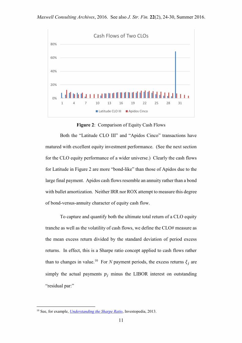
Figure 2 graphs the quarterly equity cash flows for two comparable

CLO transactions as fractions of original par amount. Both equity tranches

have healthy per annum IRR and ROX values – roughly 25% and 19%,

respectively.


11

Figure 2: Comparison of Equity Cash Flows

Both the “Latitude CLO III” and “Apidos Cinco” transactions have

matured with excellent equity investment performance. (See the next section

for the CLO equity performance of a wider universe.) Clearly the cash flows

for Latitude in Figure 2 are more “bond-like” than those of Apidos due to the

large final payment. Apidos cash flows resemble an annuity rather than a bond

with bullet amortization. Neither IRR nor ROX attempt to measure this degree

of bond-versus-annuity character of equity cash flow.

To capture and quantify both the ultimate total return of a CLO equity

tranche as well as the volatility of cash flows, we define the CLO# measure as

the mean excess return divided by the standard deviation of period excess

returns. In effect, this is a Sharpe ratio concept applied to cash flows rather

than to changes in value.10 For N payment periods, the excess returns 𝜉𝑗 are

simply the actual payments 𝑝𝑗 minus the LIBOR interest on outstanding

“residual par:”

10 See, for example, Understanding the Sharpe Ratio, Investopedia, 2013.

0%

20%

40%

60%

80%

1 4 7 10 13 16 19 22 25 28 31

Cash Flows of Two CLOs

Latitude CLO III Apidos Cinco

http://www.investopedia.com/articles/07/sharpe_ratio.asp


12

𝜉𝑗 = 𝑝𝑗 − 𝜓𝑗−1 𝐿𝑗−1 (𝑡𝑗 − 𝑡𝑗−1) , 𝑗 = 1, ⋯ , 𝑁 . (5𝑎)

𝜓0 = 𝜙0, 𝜓𝑗 = 𝜓𝑗−1 − 𝜉𝑗 , 𝑗 = 1, ⋯ , 𝑁 . (5𝑏)

In equation (5a), 𝐿𝑗−1 is the LIBOR setting for the time period 𝑡𝑗−1 to

𝑡𝑗. Equation (5b) shows our creation of a “residual par” 𝜓𝑗. While there’s no

meaningful distinction between interest and principal for equity cash flows,

we do need to track the effective return of invested funds. Thus, we imagine

that excess returns pay down this residual par. This residual par is essentially

a funding note for the purchase of the equity tranche. Augmenting the

equation (5a) definition of 𝜉𝑗, we subtract the ending residual par 𝜓𝑁 for the

excess return 𝜉𝑁.

Given this specification for the excess returns 𝜉𝑗 of CLO equity cash

flows, our volatility measure is:

CLO# = 𝑀𝑒𝑎𝑛 {𝜉𝑗} 𝑆𝑡𝑑 𝐷𝑒𝑣 {𝜉𝑗}⁄ . (6)

Evaluating this result for our two CLO equity investments of Figure 2,

we find CLO# values of 3.0 and 0.69 for “Apidos Cinco” and “Latitude CLO

III”, respectively. When comparing the CLO# of two transactions, larger is

better when investment returns are similar. The next section presents a list of

matured CLO equity investments sorted by best ROX and CLO#.

Application to large library of past equity tranches of CLOi

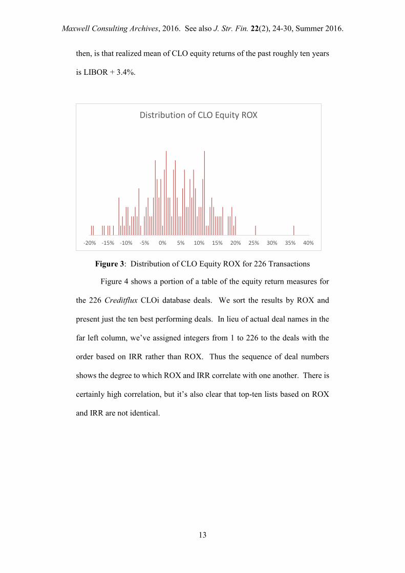
From the Creditflux CLOi deal database we have chosen 226 matured

transactions based on currency (USD), year of closing (2003 and later), and

other considerations pertaining to available data. Figure 3 plots the ROX of

the CLO equity investments. The mean ROX is essentially identical to the

median at 3.4%. The sample standard deviation is 8.9%. A headline result,

http://cloi.creditflux.com/


13

then, is that realized mean of CLO equity returns of the past roughly ten years

is LIBOR + 3.4%.

Figure 3: Distribution of CLO Equity ROX for 226 Transactions

Figure 4 shows a portion of a table of the equity return measures for

the 226 Creditflux CLOi database deals. We sort the results by ROX and

present just the ten best performing deals. In lieu of actual deal names in the

far left column, we’ve assigned integers from 1 to 226 to the deals with the

order based on IRR rather than ROX. Thus the sequence of deal numbers

shows the degree to which ROX and IRR correlate with one another. There is

certainly high correlation, but it’s also clear that top-ten lists based on ROX

and IRR are not identical.

-20% -15% -10% -5% 0% 5% 10% 15% 20% 25% 30% 35% 40%

Distribution of CLO Equity ROX


14

Deal Closing IRR ROX CLO#

1 2006 40.9% 36.1% 2.59

2 2007 30.2% 25.6% 1.48

3 2007 25.8% 20.2% 3.41

6 2007 24.6% 20.0% 2.66

22 2007 18.6% 19.5% 0.60

11 2005 21.3% 19.2% 0.58

7 2011 22.8% 19.0% 0.74

8 2007 22.7% 18.9% 0.69

18 2007 19.8% 18.6% 0.48

5 2007 25.3% 18.5% 3.04

Figure 4: Comparison of IRR, ROX, and CLO# Values

Figure 5 sorts all 226 CLO transactions and presents just the ten best

performing tranches in terms of CLO#. Interestingly, this selection by ratio

of excess returns to variability of returns produces a significantly different

sense of “best deals” than either ROX or IRR alone. All of these “top ten”

have attractive ROX values, but the ordering of deal performance differs

greatly.

Deal Closing Payment IRR ROX CLO#

42 2011 10/20/2015 16.2% 8.6% 4.80

121 2011 10/21/2015 6.4% 3.5% 4.56

3 2007 11/27/2015 25.8% 20.2% 3.41

28 2006 12/12/2012 18.2% 11.4% 3.13

5 2007 11/16/2015 25.3% 18.5% 3.04

9 2007 12/21/2015 22.7% 16.5% 3.03

14 2007 11/18/2015 20.8% 14.6% 2.98

33 2005 4/27/2015 17.8% 9.0% 2.80

6 2007 12/22/2015 24.6% 20.0% 2.66

29 2005 11/18/2013 18.0% 10.5% 2.66

Figure 5: Comparison of Equity Cash Flows Sorted by CLO#


15

Summary

After describing CLO equity tranches as an investment class, we

explained in some detail the industry-standard IRR calculation to measure,

either retrospectively or on a pro forma projected basis, investment

performance. This IRR technique has the advantage of familiarity to

investors. Yet it also has the shortcoming of failing to distinguish performance

in high and low interest rate environments. IRR also gives non-intuitive

relative assessments when investments are at zero or negative yields.

As an improvement, we propose ROX (“return on exposure”) as a

retrospective or prospective measure of CLO equity performance. Most

importantly, ROX is more suitable to typical CLO structures in which most

assets pay LIBOR-based interest and most debt payment obligations (senior

to equity, of course) require LIBOR-based payments. Equity returns will

naturally rise and fall with LIBOR fluctuations. ROX is a superior return

measure for CLO equity since it will effectively remove the influence of

LIBOR movements. It is performance above LIBOR that is meaningful to

investors.

As one further observation, CLO equity cash flows are not “bond-

like.” There is no distinction between interest and principal for the equity

payments. One expects equity cash flows to be far more volatile than those of

any CLO debt tranche since equity payments are differences between larger

par value asset and liability cash flows. Investors, however, prefer low

volatility over high volatility – all else equal. Skillful CLO managers and

well-designed structures may well impact transactions through lower volatility


16

in equity payments. For this reason, we propose, derive, and explain the CLO#

measure as an additional assessment for CLO equity performance.

To demonstrate all three measures (ROX, IRR, CLO#), we download

necessary deal information from the Creditflux CLOi database for 226

matured transactions. Through tables and graphs we present our findings.

One particularly interesting result is that mean CLO equity returns beginning

with the 2003 vintage have been roughly LIBOR + 3.4%.

better measurements for clo equity performance

Documents