[email protected] department of computer science … · bellet, habrard and sebban (lajugie et al.,...
TRANSCRIPT

arX
iv:1
306.
6709
v4 [
cs.L
G]
12
Feb
2014
Technical report
A Survey on Metric Learning for Feature Vectors and
Structured Data
Aurelien Bellet∗ [email protected]
Department of Computer ScienceUniversity of Southern CaliforniaLos Angeles, CA 90089, USA
Amaury Habrard [email protected]
Marc Sebban [email protected]
Laboratoire Hubert Curien UMR 5516
Universite de Saint-Etienne
18 rue Benoit Lauras, 42000 St-Etienne, France
Abstract
The need for appropriate ways to measure the distance or similarity between data is ubiq-uitous in machine learning, pattern recognition and data mining, but handcrafting suchgood metrics for specific problems is generally difficult. This has led to the emergence ofmetric learning, which aims at automatically learning a metric from data and has attracteda lot of interest in machine learning and related fields for the past ten years. This surveypaper proposes a systematic review of the metric learning literature, highlighting the prosand cons of each approach. We pay particular attention to Mahalanobis distance metriclearning, a well-studied and successful framework, but additionally present a wide range ofmethods that have recently emerged as powerful alternatives, including nonlinear metriclearning, similarity learning and local metric learning. Recent trends and extensions, suchas semi-supervised metric learning, metric learning for histogram data and the derivation ofgeneralization guarantees, are also covered. Finally, this survey addresses metric learningfor structured data, in particular edit distance learning, and attempts to give an overviewof the remaining challenges in metric learning for the years to come.
Keywords: Metric Learning, Similarity Learning, Mahalanobis Distance, Edit Distance
1. Introduction
The notion of pairwise metric—used throughout this survey as a generic term for distance,similarity or dissimilarity function—between data points plays an important role in manymachine learning, pattern recognition and data mining techniques.1 For instance, in classi-fication, the k-Nearest Neighbor classifier (Cover and Hart, 1967) uses a metric to identifythe nearest neighbors; many clustering algorithms, such as the prominent K-Means (Lloyd,1982), rely on distance measurements between data points; in information retrieval, doc-
∗. Most of the work in this paper was carried out while the author was affiliated with Laboratoire HubertCurien UMR 5516, Universite de Saint-Etienne, France.
1. Metric-based learning methods were the focus of the recent SIMBAD European project (ICT 2008-FET2008-2011). Website: http://simbad-fp7.eu/
c© Aurelien Bellet, Amaury Habrard and Marc Sebban.

Bellet, Habrard and Sebban
uments are often ranked according to their relevance to a given query based on similarityscores. Clearly, the performance of these methods depends on the quality of the metric:as in the saying “birds of a feather flock together”, we hope that it identifies as similar(resp. dissimilar) the pairs of instances that are indeed semantically close (resp. different).General-purpose metrics exist (e.g., the Euclidean distance and the cosine similarity forfeature vectors or the Levenshtein distance for strings) but they often fail to capture theidiosyncrasies of the data of interest. Improved results are expected when the metric isdesigned specifically for the task at hand. Since manual tuning is difficult and tedious, a lotof effort has gone into metric learning, the research topic devoted to automatically learningmetrics from data.
1.1 Metric Learning in a Nutshell
Although its origins can be traced back to some earlier work (e.g., Short and Fukunaga,1981; Fukunaga, 1990; Friedman, 1994; Hastie and Tibshirani, 1996; Baxter and Bartlett,1997), metric learning really emerged in 2002 with the pioneering work of Xing et al. (2002)that formulates it as a convex optimization problem. It has since been a hot research topic,being the subject of tutorials at ICML 20102 and ECCV 20103 and workshops at ICCV2011,4 NIPS 20115 and ICML 2013.6
The goal of metric learning is to adapt some pairwise real-valued metric function, saythe Mahalanobis distance dM (x,x′) =
√
(x− x′)TM(x− x′), to the problem of interestusing the information brought by training examples. Most methods learn the metric (here,the positive semi-definite matrix M in dM ) in a weakly-supervised way from pair or triplet-based constraints of the following form:
• Must-link / cannot-link constraints (sometimes called positive / negative pairs):
S = (xi, xj) : xi and xj should be similar,D = (xi, xj) : xi and xj should be dissimilar.
• Relative constraints (sometimes called training triplets):
R = (xi, xj , xk) : xi should be more similar to xj than to xk.
A metric learning algorithm basically aims at finding the parameters of the metric suchthat it best agrees with these constraints (see Figure 1 for an illustration), in an effort toapproximate the underlying semantic metric. This is typically formulated as an optimizationproblem that has the following general form:
minM
ℓ(M ,S,D,R) + λR(M)
where ℓ(M ,S,D,R) is a loss function that incurs a penalty when training constraintsare violated, R(M ) is some regularizer on the parameters M of the learned metric and
2. http://www.icml2010.org/tutorials.html3. http://www.ics.forth.gr/eccv2010/tutorials.php4. http://www.iccv2011.org/authors/workshops/5. http://nips.cc/Conferences/2011/Program/schedule.php?Session=Workshops6. http://icml.cc/2013/?page_id=41
2

A Survey on Metric Learning for Feature Vectors and Structured Data
Metric Learning
Figure 1: Illustration of metric learning applied to a face recognition task. For simplicity,images are represented as points in 2 dimensions. Pairwise constraints, shownin the left pane, are composed of images representing the same person (must-link, shown in green) or different persons (cannot-link, shown in red). We wishto adapt the metric so that there are fewer constraint violations (right pane).Images are taken from the Caltech Faces dataset.8
Underlying
distribution
Metric learning
algorithm
Metric-based
algorithm
Data
sample
Learned
metric
Learned
predictorPrediction
Figure 2: The common process in metric learning. A metric is learned from training dataand plugged into an algorithm that outputs a predictor (e.g., a classifier, a regres-sor, a recommender system...) which hopefully performs better than a predictorinduced by a standard (non-learned) metric.
λ ≥ 0 is the regularization parameter. As we will see in this survey, state-of-the-art metriclearning formulations essentially differ by their choice of metric, constraints, loss functionand regularizer.
After the metric learning phase, the resulting function is used to improve the perfor-mance of a metric-based algorithm, which is most often k-Nearest Neighbors (k-NN), butmay also be a clustering algorithm such as K-Means, a ranking algorithm, etc. The commonprocess in metric learning is summarized in Figure 2.
1.2 Applications
Metric learning can potentially be beneficial whenever the notion of metric between in-stances plays an important role. Recently, it has been applied to problems as diverse aslink prediction in networks (Shaw et al., 2011), state representation in reinforcement learn-ing (Taylor et al., 2011), music recommendation (McFee et al., 2012), partitioning problems
8. http://www.vision.caltech.edu/html-files/archive.html
3

Bellet, Habrard and Sebban
(Lajugie et al., 2014), identity verification (Ben et al., 2012), webpage archiving (Law et al.,2012), cartoon synthesis (Yu et al., 2012) and even assessing the efficacy of acupuncture(Liang et al., 2012), to name a few. In the following, we list three large fields of applicationwhere metric learning has been shown to be very useful.
Computer vision There is a great need of appropriate metrics in computer vision, notonly to compare images or videos in ad-hoc representations—such as bags-of-visual-words(Li and Perona, 2005)—but also in the pre-processing step consisting in building this veryrepresentation (for instance, visual words are usually obtained by means of clustering). Forthis reason, there exists a large body of metric learning literature dealing specifically withcomputer vision problems, such as image classification (Mensink et al., 2012), object recog-nition (Frome et al., 2007; Verma et al., 2012), face recognition (Guillaumin et al., 2009b;Lu et al., 2012), visual tracking (Li et al., 2012; Jiang et al., 2012) or image annotation(Guillaumin et al., 2009a).
Information retrieval The objective of many information retrieval systems, such assearch engines, is to provide the user with the most relevant documents according to his/herquery. This ranking is often achieved by using a metric between two documents or betweena document and a query. Applications of metric learning to these settings include the workof Lebanon (2006); Lee et al. (2008); McFee and Lanckriet (2010); Lim et al. (2013).
Bioinformatics Many problems in bioinformatics involve comparing sequences such asDNA, protein or temporal series. These comparisons are based on structured metrics suchas edit distance measures (or related string alignment scores) for strings or Dynamic TimeWarping distance for temporal series. Learning these metrics to adapt them to the taskof interest can greatly improve the results. Examples include the work of Xiong and Chen(2006); Saigo et al. (2006); Kato and Nagano (2010); Wang et al. (2012a).
1.3 Related Topics
We mention here three research topics that are related to metric learning but outside thescope of this survey.
Kernel learning While metric learning is parametric (one learns the parameters of agiven form of metric, such as a Mahalanobis distance), kernel learning is usually nonpara-metric: one learns the kernel matrix without any assumption on the form of the kernelthat implicitly generated it. These approaches are thus very powerful but limited to thetransductive setting and can hardly be applied to new data. The interested reader mayrefer to the recent survey on kernel learning by Abbasnejad et al. (2012).
Multiple kernel learning Unlike kernel learning, Multiple Kernel Learning (MKL) isparametric: it learns a combination of predefined base kernels. In this regard, it can be seenas more restrictive than metric or kernel learning, but as opposed to kernel learning, MKLhas very efficient formulations and can be applied in the inductive setting. The interestedreader may refer to the recent survey on MKL by Gonen and Alpaydin (2011).
Dimensionality reduction Supervised dimensionality reduction aims at finding a low-dimensional representation that maximizes the separation of labeled data and in this respect
4

A Survey on Metric Learning for Feature Vectors and Structured Data
has connections with metric learning,9 although the primary objective is quite different.Unsupervised dimensionality reduction, or manifold learning, usually assume that the (un-labeled) data lie on an embedded low-dimensional manifold within the higher-dimensionalspace and aim at “unfolding” it. These methods aim at capturing or preserving some prop-erties of the original data (such as the variance or local distance measurements) in thelow-dimensional representation.10 The interested reader may refer to the surveys by Fodor(2002) and van der Maaten et al. (2009).
1.4 Why this Survey?
As pointed out above, metric learning has been a hot topic of research in machine learningfor a few years and has now reached a considerable level of maturity both practically andtheoretically. The early review due to Yang and Jin (2006) is now largely outdated as itmisses out on important recent advances: more than 75% of the work referenced in thepresent survey is post 2006. A more recent survey, written independently and in parallel toour work, is due to Kulis (2012). Despite some overlap, it should be noted that both surveyshave their own strengths and complement each other well. Indeed, the survey of Kulis takesa more general approach, attempting to provide a unified view of a few core metric learningmethods. It also goes into depth about topics that are only briefly reviewed here, suchas kernelization, optimization methods and applications. On the other hand, the presentsurvey is a detailed and comprehensive review of the existing literature, covering more than50 approaches (including many recent works that are missing from Kulis’ paper) with theirrelative merits and drawbacks. Furthermore, we give particular attention to topics thatare not covered by Kulis, such as metric learning for structured data and the derivation ofgeneralization guarantees.
We think that the present survey may foster novel research in metric learning and beuseful to a variety of audiences, in particular: (i) machine learners wanting to get introducedto or update their knowledge of metric learning will be able to quickly grasp the pros andcons of each method as well as the current strengths and limitations of the research areaas a whole, and (ii) machine learning practitioners interested in applying metric learning totheir own problem will find information to help them choose the methods most appropriateto their needs, along with links to source codes whenever available.
Note that we focus on general-purpose methods, i.e., that are applicable to a wide rangeof application domains. The abundant literature on metric learning designed specifically forcomputer vision is not addressed because the understanding of these approaches requires asignificant amount of background in that area. For this reason, we think that they deservea separate survey, targeted at the computer vision audience.
1.5 Prerequisites
This survey is almost self-contained and has few prerequisites. For metric learning fromfeature vectors, we assume that the reader has some basic knowledge of linear algebra
9. Some metric learning methods can be seen as finding a new feature space, and a few of them actuallyhave the additional goal of making this feature space low-dimensional.
10. These approaches are sometimes referred to as “unsupervised metric learning”, which is somewhat mis-leading because they do not optimize a notion of metric.
5

Bellet, Habrard and Sebban
Notation Description
R Set of real numbers
Rd Set of d-dimensional real-valued vectors
Rc×d Set of c× d real-valued matrices
Sd+
Cone of symmetric PSD d× d real-valued matrices
X Input (instance) space
Y Output (label) space
S Set of must-link constraints
D Set of cannot-link constraints
R Set of relative constraints
z = (x, y) ∈ X × Y An arbitrary labeled instance
x An arbitrary vector
M An arbitrary matrix
I Identity matrix
M 0 PSD matrix M
‖ · ‖p p-norm
‖ · ‖F Frobenius norm
‖ · ‖∗ Nuclear norm
tr(M) Trace of matrix M
[t]+ = max(0, 1− t) Hinge loss function
ξ Slack variable
Σ Finite alphabet
x String of finite size
Table 1: Summary of the main notations.
and convex optimization (if needed, see Boyd and Vandenberghe, 2004, for a brush-up).For metric learning from structured data, we assume that the reader has some familiaritywith basic probability theory, statistics and likelihood maximization. The notations usedthroughout this survey are summarized in Table 1.
1.6 Outline
The rest of this paper is organized as follows. We first assume that data consist of vectorslying in some feature space X ⊆ R
d. Section 2 describes key properties that we will useto provide a taxonomy of metric learning algorithms. In Section 3, we review the largebody of work dealing with supervised Mahalanobis distance learning. Section 4 deals withrecent advances and trends in the field, such as linear similarity learning, nonlinear andlocal methods, histogram distance learning, the derivation of generalization guarantees andsemi-supervised metric learning methods. We cover metric learning for structured datain Section 5, with a focus on edit distance learning. Lastly, we conclude this survey inSection 6 with a discussion on the current limitations of the existing literature and promisingdirections for future research.
2. Key Properties of Metric Learning Algorithms
Except for a few early methods, most metric learning algorithms are essentially “com-petitive” in the sense that they are able to achieve state-of-the-art performance on someproblems. However, each algorithm has its intrinsic properties (e.g., type of metric, abilityto leverage unsupervised data, good scalability with dimensionality, generalization guaran-
6

A Survey on Metric Learning for Feature Vectors and Structured Data
Metric Learning
Fully
supervised
Weakly
supervised
Semi
supervised
Learning
paradigm
Form of
metric
Linear
Nonlinear
Local
Optimality of
the solution
Local
Global
Scalability
w.r.t.
dimension
w.r.t. number
of examples
Dimensionality
reduction
Yes
No
Figure 3: Five key properties of metric learning algorithms.
tees, etc) and emphasis should be placed on those when deciding which method to applyto a given problem. In this section, we identify and describe five key properties of metriclearning algorithms, summarized in Figure 3. We use them to provide a taxonomy of theexisting literature: the main features of each method are given in Table 2.11
Learning Paradigm We will consider three learning paradigms:
• Fully supervised: the metric learning algorithm has access to a set of labeled traininginstances zi = (xi, yi)ni=1, where each training example zi ∈ Z = X ×Y is composedof an instance xi ∈ X and a label (or class) yi ∈ Y. Y is a discrete and finite set of|Y| labels (unless stated otherwise). In practice, the label information is often usedto generate specific sets of pair/triplet constraints S,D,R, for instance based on anotion of neighborhood.12
• Weakly supervised: the algorithm has no access to the labels of individual traininginstances: it is only provided with side information in the form of sets of constraintsS,D,R. This is a meaningful setting in a variety of applications where labeled data iscostly to obtain while such side information is cheap: examples include users’ implicitfeedback (e.g., clicks on search engine results), citations among articles or links in anetwork. This can be seen as having label information only at the pair/triplet level.
• Semi-supervised: besides the (full or weak) supervision, the algorithm has access toa (typically large) sample of unlabeled instances for which no side information isavailable. This is useful to avoid overfitting when the labeled data or side informationare scarce.
Form of Metric Clearly, the form of the learned metric is a key choice. One may identifythree main families of metrics:
11. Whenever possible, we use the acronyms provided by the authors of the studied methods. When thereis no known acronym, we take the liberty of choosing one.
12. These constraints are usually derived from the labels prior to learning the metric and never challenged.Note that Wang et al. (2012b) propose a more refined (but costly) approach to the problem of buildingthe constraints from labels. Their method alternates between selecting the most relevant constraintsgiven the current metric and learning a new metric based on the current constraints.
7

Bellet, Habrard and Sebban
• Linear metrics, such as the Mahalanobis distance. Their expressive power is limitedbut they are easier to optimize (they usually lead to convex formulations, and thusglobal optimality of the solution) and less prone to overfitting.
• Nonlinear metrics, such as the χ2 histogram distance. They often give rise to noncon-vex formulations (subject to local optimality) and may overfit, but they can capturenonlinear variations in the data.
• Local metrics, where multiple (linear or nonlinear) local metrics are learned (typicallysimultaneously) to better deal with complex problems, such as heterogeneous data.They are however more prone to overfitting than global methods since the number ofparameters they learn can be very large.
Scalability With the amount of available data growing fast, the problem of scalabilityarises in all areas of machine learning. First, it is desirable for a metric learning algorithm toscale well with the number of training examples n (or constraints). As we will see, learningthe metric in an online way is one of the solutions. Second, metric learning methodsshould also scale reasonably well with the dimensionality d of the data. However, sincemetric learning is often phrased as learning a d× d matrix, designing algorithms that scalereasonably well with this quantity is a considerable challenge.
Optimality of the Solution This property refers to the ability of the algorithm to findthe parameters of the metric that satisfy best the criterion of interest. Ideally, the solutionis guaranteed to be the global optimum—this is essentially the case for convex formulationsof metric learning. On the contrary, for nonconvex formulations, the solution may only bea local optimum.
Dimensionality Reduction As noted earlier, metric learning is sometimes formulatedas finding a projection of the data into a new feature space. An interesting byproduct inthis case is to look for a low-dimensional projected space, allowing faster computations aswell as more compact representations. This is typically achieved by forcing or regularizingthe learned metric matrix to be low-rank.
3. Supervised Mahalanobis Distance Learning
This section deals with (fully or weakly) supervised Malahanobis distance learning (some-times simply referred to as distance metric learning), which has attracted a lot of interestdue to its simplicity and nice interpretation in terms of a linear projection. We start bypresenting the Mahalanobis distance and two important challenges associated with learningthis form of metric.
The Mahalanobis distance This term comes from Mahalanobis (1936) and originallyrefers to a distance measure that incorporates the correlation between features:
dmaha(x,x′) =
√
(x− x′)TΩ−1(x− x′),
where x and x′ are random vectors from the same distribution with covariance matrix Ω.By an abuse of terminology common in the metric learning literature, we will in fact use
8

ASurveyonMetric
Learning
forFeatureVectorsandStructured
Data
Page Name YearSource
SupervisionForm of Scalability
OptimumDimension
RegularizerAdditional
Code Metric w.r.t. n w.r.t. d Reduction Information
11 MMC 2002 Yes Weak Linear Global No None —
11 S&J 2003 No Weak Linear Global No Frobenius norm —
12 NCA 2004 Yes Full Linear Local Yes None For k-NN
12 MCML 2005 Yes Full Linear Global No None For k-NN
13 LMNN 2005 Yes Full Linear Global No None For k-NN
13 RCA 2003 Yes Weak Linear Global No None —
14 ITML 2007 Yes Weak Linear Global No LogDet Online version
15 SDML 2009 No Weak Linear Global No LogDet+L1 n ≪ d
15 POLA 2004 No Weak Linear Global No None Online
15 LEGO 2008 No Weak Linear Global No LogDet Online
16 RDML 2009 No Weak Linear Global No Frobenius norm Online
16 MDML 2012 No Weak Linear Global Yes Nuclear norm Online
16 mt-LMNN 2010 Yes Full Linear Global No Frobenius norm Multi-task
17 MLCS 2011 No Weak Linear Local Yes N/A Multi-task
17 GPML 2012 No Weak Linear Global Yes von Neumann Multi-task
18 TML 2010 Yes Weak Linear Global No Frobenius norm Transfer learning
19 LPML 2006 No Weak Linear Global Yes L1 norm —
19 SML 2009 No Weak Linear Global Yes L2,1 norm —
19 BoostMetric 2009 Yes Weak Linear Global Yes None —
20 DML-p 2012 No Weak Linear Global No None —
20 RML 2010 No Weak Linear Global No Frobenius norm Noisy constraints
21 MLR 2010 Yes Full Linear Global Yes Nuclear norm For ranking
22 SiLA 2008 No Full Linear N/A No None Online
22 gCosLA 2009 No Weak Linear Global No None Online
23 OASIS 2009 Yes Weak Linear Global No Frobenius norm Online
23 SLLC 2012 No Full Linear Global No Frobenius norm For linear classif.
24 RSL 2013 No Full Linear Local No Frobenius norm Rectangular matrix
25 LSMD 2005 No Weak Nonlinear Local Yes None —
25 NNCA 2007 No Full Nonlinear Local Yes Recons. error —
26 SVML 2012 No Full Nonlinear Local Yes Frobenius norm For SVM
26 GB-LMNN 2012 No Full Nonlinear Local Yes None —
26 HDML 2012 Yes Weak Nonlinear Local Yes L2 norm Hamming distance
27 M2-LMNN 2008 Yes Full Local Global No None —
28 GLML 2010 No Full Local Global No Diagonal Generative
28 Bk-means 2009 No Weak Local Global No RKHS norm Bregman dist.
29 PLML 2012 Yes Weak Local Global No Manifold+Frob —
29 RFD 2012 Yes Weak Local N/A No None Random forests
30 χ2-LMNN 2012 No Full Nonlinear Local Yes None Histogram data
31 GML 2011 No Weak Linear Local No None Histogram data
31 EMDL 2012 No Weak Linear Local No Frobenius norm Histogram data
34 LRML 2008 Yes Semi Linear Global No Laplacian —
35 M-DML 2009 No Semi Linear Local No Laplacian Auxiliary metrics
35 SERAPH 2012 Yes Semi Linear Local Yes Trace+entropy Probabilistic
36 CDML 2011 No Semi N/A N/A N/A N/A N/A N/A Domain adaptation
36 DAML 2011 No Semi Nonlinear Global No MMD Domain adaptation
Table 2: Main features of metric learning methods for feature vectors. Scalability levels are relative and given as a rough guide.
9

Bellet, Habrard and Sebban
the term Mahalanobis distance to refer to generalized quadratic distances, defined as
dM (x,x′) =√
(x− x′)TM (x− x′)
and parameterized by M ∈ Sd+, where S
d+ is the cone of symmetric positive semi-definite
(PSD) d × d real-valued matrices (see Figure 4).13 M ∈ Sd+ ensures that dM satisfies the
properties of a pseudo-distance: ∀x,x′,x′′ ∈ X ,
1. dM (x,x′) ≥ 0 (nonnegativity),
2. dM (x,x) = 0 (identity),
3. dM (x,x′) = d(x′,x) (symmetry),
4. dM (x,x′′) ≤ d(x,x′) + d(x′,x′′) (triangle inequality).
Interpretation Note that when M is the identity matrix, we recover the Euclideandistance. Otherwise, one can express M as LTL, where L ∈ R
k×d where k is the rank ofM . We can then rewrite dM (x,x′) as follows:
dM (x,x′) =√
(x− x′)TM (x− x′)
=
√
(x− x′)TLTL(x− x′)
=√
(Lx−Lx′)T (Lx−Lx′).
Thus, a Mahalanobis distance implicitly corresponds to computing the Euclidean distanceafter the linear projection of the data defined by the transformation matrix L. Note thatif M is low-rank, i.e., rank(M ) = r < d, then it induces a linear projection of the datainto a space of lower dimension r. It thus allows a more compact representation of thedata and cheaper distance computations, especially when the original feature space is high-dimensional. These nice properties explain why learning Mahalanobis distance has attracteda lot of interest and is a major component of metric learning.
Challenges This leads us to two important challenges associated with learning Maha-lanobis distances. The first one is to maintain M ∈ S
d+ in an efficient way during the
optimization process. A simple way to do this is to use the projected gradient methodwhich consists in alternating between a gradient step and a projection step onto the PSDcone by setting the negative eigenvalues to zero.14 However this is expensive for high-dimensional problems as eigenvalue decomposition scales in O(d3). The second challengeis to learn a low-rank matrix (which implies a low-dimensional projection space, as notedearlier) instead of a full-rank one. Unfortunately, optimizing M subject to a rank constraintor regularization is NP-hard and thus cannot be carried out efficiently.
13. Note that in practice, to get rid of the square root, the Mahalanobis distance is learned in its moreconvenient squared form d2M (x,x′) = (x− x
′)TM(x− x′).
14. Note that Qian et al. (2013) have proposed some heuristics to avoid doing this projection at each itera-tion.
10

A Survey on Metric Learning for Feature Vectors and Structured Data
00.2
0.40.6
0.81
−1
−0.5
0
0.5
10
0.2
0.4
0.6
0.8
1
αβ
γ
Figure 4: The cone S2+ of positive semi-definite 2x2 matrices of the form
[
α β
β γ
]
.
The rest of this section is a comprehensive review of the supervised Mahalanobis distancelearning methods of the literature. We first present two early approaches (Section 3.1). Wethen discuss methods that are specific to k-nearest neighbors (Section 3.2), inspired from in-formation theory (Section 3.3), online learning approaches (Section 3.4), multi-task learning(Section 3.5) and a few more that do not fit any of the previous categories (Section 3.6).
3.1 Early Approaches
The approaches in this section deal with the PSD constraint in a rudimentary way.
MMC (Xing et al.) The seminal work of Xing et al. (2002) is the first Mahalanobisdistance learning method.15 It relies on a convex formulation with no regularization, whichaims at maximizing the sum of distances between dissimilar points while keeping the sumof distances between similar examples small:
maxM∈Sd
+
∑
(xi,xj)∈D
dM (xi,xj)
s.t.∑
(xi,xj)∈S
d2M (xi,xj) ≤ 1.(1)
The algorithm used to solve (1) is a simple projected gradient approach requiring the fulleigenvalue decomposition of M at each iteration. This is typically intractable for mediumand high-dimensional problems.
S&J (Schultz & Joachims) The method proposed by Schultz and Joachims (2003) re-lies on the parameterization M = ATWA, where A is fixed and known and W diagonal.We get:
d2M (xi,xj) = (Axi −Axj)TW (Axi −Axj).
15. Source code available at: http://www.cs.cmu.edu/~epxing/papers/
11

Bellet, Habrard and Sebban
By definition, M is PSD and thus one can optimize over the diagonal matrix W and avoidthe need for costly projections on the PSD cone. They propose a formulation based ontriplet constraints:
minW
‖M‖2F + C∑
i,j,k
ξijk
s.t. d2M (xi,xk)− d2M (xi,xj) ≥ 1− ξijk ∀(xi,xj ,xk) ∈ R,(2)
where ‖M‖2F =∑
i,jM2ij is the squared Frobenius norm of M , the ξijk’s are “slack” vari-
ables to allow soft constraints16 and C ≥ 0 is the trade-off parameter between regularizationand constraint satisfaction. Problem (2) is convex and can be solved efficiently. The maindrawback of this approach is that it is less general than full Mahalanobis distance learning:one only learns a weighting W of the features. Furthermore, A must be chosen manually.
3.2 Approaches Driven by Nearest Neighbors
The objective functions of the methods presented in this section are related to a nearestneighbor prediction rule.
NCA (Goldberger et al.) The idea of Neighbourhood Component Analysis17 (NCA),introduced by Goldberger et al. (2004), is to optimize the expected leave-one-out error of astochastic nearest neighbor classifier in the projection space induced by dM . They use thedecomposition M = LTL and they define the probability that xi is the neighbor of xj by
pij =exp(−‖Lxi −Lxj‖22)
∑
l 6=i exp(−‖Lxi −Lxl‖22), pii = 0.
Then, the probability that xi is correctly classified is:
pi =∑
j:yj=yi
pij.
They learn the distance by solving:
maxL
∑
i
pi. (3)
Note that the matrix L can be chosen to be rectangular, inducing a low-rank M . The mainlimitation of (3) is that it is nonconvex and thus subject to local maxima. Hong et al. (2011)later proposed to learn a mixture of NCA metrics, while Tarlow et al. (2013) generalize NCAto k-NN with k > 1.
MCML (Globerson & Roweis) Shortly after Goldberger et al., Globerson and Roweis(2005) proposed MCML (Maximally Collapsing Metric Learning), an alternative convexformulation based on minimizing a KL divergence between pij and an ideal distribution,
16. This is a classic trick used for instance in soft-margin SVM (Cortes and Vapnik, 1995). Throughout thissurvey, we will consistently use the symbol ξ to denote slack variables.
17. Source code available at: http://www.ics.uci.edu/~fowlkes/software/nca/
12

A Survey on Metric Learning for Feature Vectors and Structured Data
which can be seen as attempting to collapse each class to a single point.18 Unlike NCA,the optimization is done with respect to the matrix M and the problem is thus convex.However, like MMC, MCML requires costly projections onto the PSD cone.
LMNN (Weinberger et al.) Large Margin Nearest Neighbors19 (LMNN), introduced byWeinberger et al. (2005; 2008; 2009), is one of the most widely-used Mahalanobis distancelearning methods and has been the subject of many extensions (described in later sections).One of the reasons for its popularity is that the constraints are defined in a local way: thek nearest neighbors (the “target neighbors”) of any training instance should belong to thecorrect class while keeping away instances of other classes (the “impostors”). The Euclideandistance is used to determine the target neighbors. Formally, the constraints are defined inthe following way:
S = (xi,xj) : yi = yj and xj belongs to the k-neighborhood of xi,R = (xi,xj,xk) : (xi,xj) ∈ S, yi 6= yk.
The distance is learned using the following convex program:
minM∈Sd
+
(1− µ)∑
(xi,xj)∈S
d2M (xi,xj) + µ∑
i,j,k
ξijk
s.t. d2M (xi,xk)− d2M (xi,xj) ≥ 1− ξijk ∀(xi,xj,xk) ∈ R,(4)
where µ ∈ [0, 1] controls the “pull/push” trade-off. The authors developed a special-purpose solver—based on subgradient descent and careful book-keeping—that is able todeal with billions of constraints. Alternative ways of solving the problem have been pro-posed (Torresani and Lee, 2006; Nguyen and Guo, 2008; Park et al., 2011; Der and Saul,2012). LMNN generally performs very well in practice, although it is sometimes prone tooverfitting due to the absence of regularization, especially in high dimension. It is also verysensitive to the ability of the Euclidean distance to select relevant target neighbors. Notethat Do et al. (2012) highlighted a relation between LMNN and Support Vector Machines.
3.3 Information-Theoretic Approaches
The methods presented in this section frame metric learning as an optimization probleminvolving an information measure.
RCA (Bar-Hillel et al.) Relevant Component Analysis20 (Shental et al., 2002; Bar-Hillel et al.,2003, 2005) makes use of positive pairs only and is based on subsets of the training exam-ples called “chunklets”. These are obtained from the set of positive pairs by applying atransitive closure: for instance, if (x1,x2) ∈ S and (x2,x3) ∈ S, then x1, x2 and x3 belongto the same chunklet. Points in a chunklet are believed to share the same label. Assuminga total of n points in k chunklets, the algorithm is very efficient since it simply amounts to
18. An implementation is available within the Matlab Toolbox for Dimensionality Reduction:http://homepage.tudelft.nl/19j49/Matlab_Toolbox_for_Dimensionality_Reduction.html
19. Source code available at: http://www.cse.wustl.edu/~kilian/code/code.html20. Source code available at: http://www.scharp.org/thertz/code.html
13

Bellet, Habrard and Sebban
computing the following matrix:
C =1
n
k∑
j=1
nj∑
i=1
(xji − mj)(xji − mj)T ,
where chunklet j consists of xjinj
i=1 and mj is its mean. Thus, RCA essentially reduces thewithin-chunklet variability in an effort to identify features that are irrelevant to the task.The inverse of C is used in a Mahalanobis distance. The authors have shown that (i) it isthe optimal solution to an information-theoretic criterion involving a mutual informationmeasure, and (ii) it is also the optimal solution to the optimization problem consisting inminimizing the within-class distances. An obvious limitation of RCA is that it cannot makeuse of the discriminative information brought by negative pairs, which explains why it isnot very competitive in practice. RCA was later extended to handle negative pairs, at thecost of a more expensive algorithm (Hoi et al., 2006; Yeung and Chang, 2006).
ITML (Davis et al.) Information-Theoretic Metric Learning21 (ITML), proposed byDavis et al. (2007), is an important work because it introduces LogDet divergence regular-ization that will later be used in several other Mahalanobis distance learning methods (e.g.,Jain et al., 2008; Qi et al., 2009). This Bregman divergence on positive definite matrices isdefined as:
Dld(M ,M0) = tr(MM−10 )− log det(MM−1
0 )− d,
where d is the dimension of the input space and M 0 is some positive definite matrix wewant to remain close to. In practice, M0 is often set to I (the identity matrix) and thusthe regularization aims at keeping the learned distance close to the Euclidean distance. Thekey feature of the LogDet divergence is that it is finite if and only if M is positive definite.Therefore, minimizing Dld(M ,M 0) provides an automatic and cheap way of preserving thepositive semi-definiteness of M . ITML is formulated as follows:
minM∈Sd
+
Dld(M ,M0) + γ∑
i,j
ξij
s.t. d2M (xi,xj) ≤ u+ ξij ∀(xi,xj) ∈ Sd2M (xi,xj) ≥ v − ξij ∀(xi,xj) ∈ D,
(5)
where u, v ∈ R are threshold parameters and γ ≥ 0 the trade-off parameter. ITML thusaims at satisfying the similarity and dissimilarity constraints while staying as close as pos-sible to the Euclidean distance (if M0 = I). More precisely, the information-theoreticinterpretation behind minimizing Dld(M ,M 0) is that it is equivalent to minimizing theKL divergence between two multivariate Gaussian distributions parameterized by M andM0. The algorithm proposed to solve (5) is efficient, converges to the global minimum andthe resulting distance performs well in practice. A limitation of ITML is that M0, thatmust be picked by hand, can have an important influence on the quality of the learneddistance. Note that Kulis et al. (2009) have shown how hashing can be used together withITML to achieve fast similarity search.
21. Source code available at: http://www.cs.utexas.edu/~pjain/itml/
14

A Survey on Metric Learning for Feature Vectors and Structured Data
SDML (Qi et al.) With Sparse Distance Metric Learning (SDML), Qi et al. (2009)specifically deal with the case of high-dimensional data together with few training samples,i.e., n ≪ d. To avoid overfitting, they use a double regularization: the LogDet divergence(using M0 = I or M 0 = Ω−1 where Ω is the covariance matrix) and L1-regularizationon the off-diagonal elements of M . The justification for using this L1-regularization istwo-fold: (i) a practical one is that in high-dimensional spaces, the off-diagonal elements ofΩ−1 are often very small, and (ii) a theoretical one suggested by a consistency result froma previous work in covariance matrix estimation (Ravikumar et al., 2011) that applies toSDML. They use a fast algorithm based on block-coordinate descent (the optimization isdone over each row of M−1) and obtain very good performance for the specific case n≪ d.
3.4 Online Approaches
In online learning (Littlestone, 1988), the algorithm receives training instances one at atime and updates at each step the current hypothesis. Although the performance of onlinealgorithms is typically inferior to batch algorithms, they are very useful to tackle large-scaleproblems that batch methods fail to address due to time and space complexity issues. Onlinelearning methods often come with regret bounds, stating that the accumulated loss sufferedalong the way is not much worse than that of the best hypothesis chosen in hindsight.22
POLA (Shalev-Shwartz et al.) POLA (Shalev-Shwartz et al., 2004), for Pseudo-metricOnline Learning Algorithm, is the first online Mahalanobis distance learning approach andlearns the matrix M as well as a threshold b ≥ 1. At each step t, POLA receives a pair(xi,xj, yij), where yij = 1 if (xi,xj) ∈ S and yij = −1 if (xi,xj) ∈ D, and performs twosuccessive orthogonal projections:
1. Projection of the current solution (M t−1, bt−1) onto the set C1 = (M , b) ∈ Rd2+1 :
[yij(d2M (xi,xj)− b) + 1]+ = 0, which is done efficiently (closed-form solution). The
constraint basically requires that the distance between two instances of same (resp.different) labels be below (resp. above) the threshold b with a margin 1. We get an
intermediate solution (M t− 1
2 , bt−1
2 ) that satisfies this constraint while staying as closeas possible to the previous solution.
2. Projection of (M t− 1
2 , bt−1
2 ) onto the set C2 = (M , b) ∈ Rd2+1 : M ∈ S
d+, b ≥ 1,
which is done rather efficiently (in the worst case, one only needs to compute the
minimal eigenvalue of M t− 1
2 ). This projects the matrix back onto the PSD cone. Wethus get a new solution (M t, bt) that yields a valid Mahalanobis distance.
A regret bound for the algorithm is provided.
LEGO (Jain et al.) LEGO (Logdet Exact Gradient Online), developed by Jain et al.(2008), is an improved version of POLA based on LogDet divergence regularization. Itfeatures tighter regret bounds, more efficient updates and better practical performance.
22. A regret bound has the following general form:∑T
t=1ℓ(ht, zt) −
∑T
t=1ℓ(h∗, zt) ≤ O(T ), where T is the
number of steps, ht is the hypothesis at time t and h∗ is the best batch hypothesis.
15

Bellet, Habrard and Sebban
RDML (Jin et al.) RDML (Jin et al., 2009) is similar to POLA in spirit but is moreflexible. At each step t, instead of forcing the margin constraint to be satisfied, it performsa gradient descent step of the following form (assuming Frobenius regularization):
M t = πSd+
(
M t−1 − λyij(xi − xj)(xi − xj)T)
,
where πSd+(·) is the projection to the PSD cone. The parameter λ implements a trade-off
between satisfying the pairwise constraint and staying close to the previous matrix M t−1.Using some linear algebra, the authors show that this update can be performed by solvinga convex quadratic program instead of resorting to eigenvalue computation like POLA.RDML is evaluated on several benchmark datasets and is shown to perform comparably toLMNN and ITML.
MDML (Kunapuli & Shavlik) MDML (Kunapuli and Shavlik, 2012), for Mirror De-scent Metric Learning, is an attempt of proposing a general framework for online Maha-lanobis distance learning. It is based on composite mirror descent (Duchi et al., 2010), whichallows online optimization of many regularized problems. It can accommodate a large classof loss functions and regularizers for which efficient updates are derived, and the algorithmcomes with a regret bound. Their study focuses on regularization with the nuclear norm(also called trace norm) introduced by Fazel et al. (2001) and defined as ‖M‖∗ =
∑
i σi,where the σi’s are the singular values of M .23 It is known to be the best convex relaxationof the rank of the matrix and thus nuclear norm regularization tends to induce low-rankmatrices. In practice, MDML has performance comparable to LMNN and ITML, is fast andsometimes induces low-rank solutions, but surprisingly the algorithm was not evaluated onlarge-scale datasets.
3.5 Multi-Task Metric Learning
This section covers Mahalanobis distance learning for the multi-task setting (Caruana,1997), where given a set of related tasks, one learns a metric for each in a coupled fashionin order to improve the performance on all tasks.
mt-LMNN (Parameswaran & Weinberger) Multi-Task LMNN24 (Parameswaran and Weinberger,2010) is a straightforward adaptation of the ideas of Multi-Task SVM (Evgeniou and Pontil,2004) to metric learning. Given T related tasks, they model the problem as learning a sharedMahalanobis metric dM0
as well as task-specific metrics dM1, . . . , dM t and define the metric
for task t asdt(x,x
′) = (x− x′)T (M 0 +M t)(x− x′).
Note that M 0 + M t 0, hence dt is a valid pseudo-metric. The LMNN formulation iseasily generalized to this multi-task setting so as to learn the metrics jointly, with a specificregularization term defined as follows:
γ0‖M 0 − I‖2F +T∑
t=1
γt‖M t‖2F ,
23. Note that when M ∈ Sd+, ‖M‖∗ = tr(M) =
∑d
i=1Mii, which is much cheaper to compute.
24. Source code available at: http://www.cse.wustl.edu/~kilian/code/code.html
16

A Survey on Metric Learning for Feature Vectors and Structured Data
where γt controls the regularization of M t. When γ0 → ∞, the shared metric dM0is simply
the Euclidean distance, and the formulation reduces to T independent LMNN formulations.On the other hand, when γt>0 → ∞, the task-specific matrices are simply zero matricesand the formulation reduces to LMNN on the union of all data. In-between these extremecases, these parameters can be used to adjust the relative importance of each metric: γ0to set the overall level of shared information, and γt to set the importance of M t withrespect to the shared metric. The formulation remains convex and can be solved using thesame efficient solver as LMNN. In the multi-task setting, mt-LMNN clearly outperformssingle-task metric learning methods and other multi-task classification techniques such asmt-SVM.
MLCS (Yang et al.) MLCS (Yang et al., 2011) is a different approach to the problemof multi-task metric learning. For each task t ∈ 1, . . . , T, the authors consider learning aMahalanobis metric
d2LT
t Lt(x,x′) = (x− x′)TLT
t Lt(x− x′) = (Ltx−Ltx′)T (Ltx−Ltx
′)
parameterized by the transformation matrix Lt ∈ Rr×d. They show that Lt can be decom-
posed into a “subspace” part Lt0 ∈ R
r×d and a “low-dimensional metric” part Rt ∈ Rr×r
such that Lt = RtLt0. The main assumption of MLCS is that all tasks share a common
subspace, i.e., ∀t, Lt0 = L0. This parameterization can be used to extend most of metric
learning methods to the multi-task setting, although it breaks the convexity of the formu-lation and is thus subject to local optima. However, as opposed to mt-LMNN, it can bemade low-rank by setting r < d and thus has many less parameters to learn. In their work,MLCS is applied to the version of LMNN solved with respect to the transformation matrix(Torresani and Lee, 2006). The resulting method is evaluated on problems with very scarcetraining data and study the performance for different values of r. It is shown to outperformmt-LMNN, but the setup is a bit unfair to mt-LMNN since it is forced to be low-rank byeigenvalue thresholding.
GPML (Yang et al.) The work of Yang et al. (2012) identifies two drawbacks of pre-vious multi-task metric learning approaches: (i) MLCS’s assumption of common subspaceis sometimes too strict and leads to a nonconvex formulation, and (ii) the Frobenius reg-ularization of mt-LMNN does not preserve geometry. This property is defined as beingthe ability to propagate side-information: the task-specific metrics should be regularized soas to preserve the relative distance between training pairs. They introduce the followingformulation, which extends any metric learning algorithm to the multi-task setting:
minM0,...,M t∈Sd+
t∑
i=1
(ℓ(M t,St,Dt,Rt) + γdϕ(M t,M 0)) + γ0dϕ(A0,M0), (6)
where ℓ(M t,St,Dt,Rt) is the loss function for the task t based on the training pairs/triplets(depending on the chosen algorithm), dϕ(A,B) = ϕ(A) − ϕ(B) − tr
(
(∇ϕB)T (A−B))
is a Bregman matrix divergence (Dhillon and Tropp, 2007) and A0 is a predefined metric(e.g., the identity matrix I). mt-LMNN can essentially be recovered from (6) by settingϕ(A) = ‖A‖2F and additional constraints M t M0. The authors focus on the von
17

Bellet, Habrard and Sebban
Neumann divergence:
dV N (A,B) = tr(A logA−A logB −A+B),
where logA is the matrix logarithm of A. Like the LogDet divergence mentioned earlier inthis survey (Section 3.3), the von Neumann divergence is known to be rank-preserving and toprovide automatic enforcement of positive-semidefiniteness. The authors further show thatminimizing this divergence encourages geometry preservation between the learned metrics.Problem (6) remains convex as long as the original algorithm used for solving each task isconvex, and can be solved efficiently using gradient descent methods. In the experiments,the method is adapted to LMNN and outperforms single-task LMNN as well as mt-LMNN,especially when training data is very scarce.
TML (Zhang & Yeung) Zhang and Yeung (2010) propose a transfer metric learning(TML) approach.25 They assume that we are given S independent source tasks with enoughlabeled data and that a Mahalanobis distanceM s has been learned for each task s. The goalis to leverage the information of the source metrics to learn a distance M t for a target task,for which we only have a scarce amount nt of labeled data. No assumption is made aboutthe relation between the source tasks and the target task: they may be positively/negativelycorrelated or uncorrelated. The problem is formulated as follows:
minM t∈Sd+,Ω0
2
n2t
∑
i<j
ℓ(
yiyj[
1− d2M t(xi,xj)
])
+λ12‖M t‖2F +
λ22
tr(MΩ−1MT)
s.t. tr(Ω) = 1,
(7)
where ℓ(t) = max(0, 1 − t) is the hinge loss, M = (vec(M1), . . . , vec(M s), vec(M t)). Thefirst two terms are classic (loss on all possible pairs and Frobenius regularization) while thethird one models the relation between tasks based on a positive definite covariance matrixΩ. Assuming that the source tasks are independent and of equal importance, Ω can beexpressed as
Ω =
(
αI(m−1)×(m−1) ωm
ωm ω
)
,
where ωm denotes the task covariances between the target task and the source tasks, andω denotes the variance of the target task. Problem (7) is convex and is solved using analternating procedure that is guaranteed to converge to the global optimum: (i) fixing Ωand solving for M t, which is done online with an algorithm similar to RDML, and (ii) fixingM t and solving for Ω, leading to a second-order cone program whose number of variablesand constraints is linear in the number of tasks. In practice, TML consistently outperformsmetric learning methods without transfer when training data is scarce.
3.6 Other Approaches
In this section, we describe a few approaches that are outside the scope of the previouscategories. The first two (LPML and SML) fall into the category of sparse metric learning
25. Source code available at: http://www.cse.ust.hk/~dyyeung/
18

A Survey on Metric Learning for Feature Vectors and Structured Data
methods. BoostMetric is inspired from the theory of boosting. DML-p revisits the originalmetric learning formulation of Xing et al. RML deals with the presence of noisy constraints.Finally, MLR learns a metric for solving a ranking task.
LPML (Rosales & Fung) The method of Rosales and Fung (2006) aims at learningmatrices with entire columns/rows set to zero, thus making M low-rank. For this purpose,they use L1 norm regularization and, restricting their framework to diagonal dominantmatrices, they are able to formulate the problem as a linear program that can be solvedefficiently. However, L1 norm regularization favors sparsity at the entry level only, notspecifically at the row/column level, even though in practice the learned matrix is sometimeslow-rank. Furthermore, the approach is less general than Mahalanobis distances due to therestriction to diagonal dominant matrices.
SML (Ying et al.) SML26 (Ying et al., 2009), for Sparse Metric Learning, is a distancelearning approach that regularizes M with the mixed L2,1 norm defined as
‖M‖2,1 =d∑
i=1
‖M i‖2,
which tends to zero out entire rows of M (as opposed to the L1 norm used in LPML), andtherefore performs feature selection. More precisely, they set M = UTWU , where U ∈ O
d
(the set of d× d orthonormal matrices) and W ∈ Sd+, and solve the following problem:
minU∈Od,W∈Sd+
‖W ‖2,1 + γ∑
i,j,k
ξijk
s.t. d2M (xi,xk)− d2M (xi,xj) ≥ 1− ξijk ∀(xi,xj,xk) ∈ R,(8)
where γ ≥ 0 is the trade-off parameter. Unfortunately, L2,1 regularized problems aretypically difficult to optimize. Problem (8) is reformulated as a min-max problem and solvedusing smooth optimization (Nesterov, 2005). Overall, the algorithm has a fast convergencerate but each iteration has an O(d3) complexity. The method performs well in practice whileachieving better dimensionality reduction than full-rank methods such as Rosales and Fung(2006). However, it cannot be applied to high-dimensional problems due to the complexityof the algorithm. Note that the same authors proposed a unified framework for sparsemetric learning (Huang et al., 2009, 2011).
BoostMetric (Shen et al.) BoostMetric27 (Shen et al., 2009, 2012) adapts to Maha-lanobis distance learning the ideas of boosting, where a good hypothesis is obtained througha weighted combination of so-called “weak learners” (see the recent book on this matterby Schapire and Freund, 2012). The method is based on the property that any PSD ma-trix can be decomposed into a positive linear combination of trace-one rank-one matrices.This kind of matrices is thus used as weak learner and the authors adapt the popularboosting algorithm Adaboost (Freund and Schapire, 1995) to this setting. The resulting al-gorithm is quite efficient since it does not require full eigenvalue decomposition but only the
26. Source code is not available but is indicated as “coming soon” by the authors. Check:http://www.enm.bris.ac.uk/staff/xyy/software.html
27. Source code available at: http://code.google.com/p/boosting/
19

Bellet, Habrard and Sebban
computation of the largest eigenvalue. In practice, BoostMetric achieves competitive perfor-mance but typically requires a very large number of iterations for high-dimensional datasets.Bi et al. (2011) further improve the scalability of the approach, while Liu and Vemuri (2012)introduce regularization on the weights as well as a term to reduce redundancy among theweak learners.
DML-p (Ying et al., Cao et al.) The work of Ying and Li (2012); Cao et al. (2012b)revisit MMC, the original approach of Xing et al. (2002), by investigating the followingformulation, called DML-p:
maxM∈Sd
+
1
|D|∑
(xi,xj)∈D
[dM (xi,xj)]2p
1/p
s.t.∑
(xi,xj)∈S
d2M (xi,xj) ≤ 1.
(9)
Note that by setting p = 0.5 we recover MMC. The authors show that (9) is convex forp ∈ (−∞, 1) and can be cast as a well-known eigenvalue optimization problem called “min-imizing the maximal eigenvalue of a symmetric matrix”. They further show that it canbe solved efficiently using a first-order algorithm that only requires the computation of thelargest eigenvalue at each iteration (instead of the costly full eigen-decomposition used byXing et al.). Experiments show competitive results and low computational complexity. Ageneral drawback of DML-p is that it is not clear how to accommodate a regularizer (e.g.,sparse or low-rank).
RML (Huang et al.) Robust Metric Learning (Huang et al., 2010) is a method thatcan successfully deal with the presence of noisy/incorrect training constraints, a situationthat can arise when they are not derived from class labels but from side information suchas users’ implicit feedback. The approach is based on robust optimization (Ben-Tal et al.,2009): assuming that a proportion 1 − η of the m training constraints (say triplets) areincorrect, it minimizes some loss function ℓ for any η fraction of the triplets:
minM∈Sd
+,t
t +λ
2‖M‖F
s.t. t ≥m∑
i=1
qiℓ(
d2M (xi,x′′
i )− d2M (xi,x′
i))
, ∀q ∈ Q(η),
(10)
where ℓ is taken to be the hinge loss and Q(η) is defined as
Q(η) =
q ∈ 0, 1m :
m∑
i=1
qi ≤ ηm
.
In other words, Problem (10) minimizes the worst-case violation over all possible sets ofcorrect constraints. Q(η) can be replaced by its convex hull, leading to a semi-definiteprogram with an infinite number of constraints. This can be further simplified into aconvex minimization problem that can be solved either using subgradient descent or smooth
20
A Survey on Metric Learning for Feature Vectors and Structured Data
optimization (Nesterov, 2005). However, both of these require a projection onto the PSDcone. Experiments on standard datasets show good robustness for up to 30% of incorrecttriplets, while the performance of other methods such as LMNN is greatly damaged.
MLR (McFee & Lankriet) The idea of MLR (McFee and Lanckriet, 2010), for MetricLearning to Rank, is to learn a metric for a ranking task, where given a query instance,one aims at producing a ranked list of examples where relevant ones are ranked higherthan irrelevant ones.28 Let P the set of all permutations (i.e., possible rankings) over thetraining set. Given a Mahalanobis distance d2M and a query x, the predicted ranking p ∈ Pconsists in sorting the instances by ascending d2M (x, ·). The metric learning M is based onStructural SVM (Tsochantaridis et al., 2005):
minM∈Sd
+
‖M‖∗ + C∑
i
ξi
s.t. 〈M , ψ(xi, pi)− ψ(xi, p)〉F ≥ ∆(pi, p)− ξi ∀i ∈ 1, . . . , n, p ∈ P,(11)
where ‖M‖∗ = tr(M ) is the nuclear norm, C ≥ 0 the trade-off parameter, 〈A,B〉F =∑
i,j AijBij the Frobenius inner product, ψ : R ×P → Sd the feature encoding of an input-
output pair (xi, p),29 and ∆(pi, p) ∈ [0, 1] the “margin” representing the loss of predicting
ranking p instead of the true ranking pi. In other words, ∆(pi, p) assesses the quality ofranking p with respect to the best ranking pi and can be evaluated using several measures,such as the Area Under the ROC Curve (AUC), Precision-at-k or Mean Average Precision(MAP). Since the number of constraints is super-exponential in the number of traininginstances, the authors solve (11) using a 1-slack cutting-plane approach (Joachims et al.,2009) which essentially iteratively optimizes over a small set of active constraints (addingthe most violated ones at each step) using subgradient descent. However, the algorithmrequires a full eigendecomposition of M at each iteration, thus MLR does not scale wellwith the dimensionality of the data. In practice, it is competitive with other metric learningalgorithms for k-NN classification and a structural SVM algorithm for ranking, and caninduce low-rank solutions due to the nuclear norm. Lim et al. (2013) propose R-MLR, anextension to MLR to deal with the presence of noisy features30 using the mixed L2,1 normas in SML (Ying et al., 2009). R-MLR is shown to be able to ignore most of the irrelevantfeatures and outperforms MLR in this situation.
4. Other Advances in Metric Learning
So far, we focused on (linear) Mahalanobis metric learning which has inspired a large amountof work during the past ten years. In this section, we cover other advances and trends inmetric learning for feature vectors. Most of the section is devoted to (fully and weakly)supervised methods. In Section 4.1, we address linear similarity learning. Section 4.2 dealswith nonlinear metric learning (including the kernelization of linear methods), Section 4.3
28. Source code is available at: http://www-cse.ucsd.edu/~bmcfee/code/mlr29. The feature map ψ is designed such that the ranking p which maximizes 〈M , ψ(x, p)〉
Fis the one given
by ascending d2M (x, ·).30. Notice that this is different from noisy side information, which was investigated by the method RML
(Huang et al., 2010) presented earlier in this section.
21

Bellet, Habrard and Sebban
with local metric learning and Section 4.4 with metric learning for histogram data. Sec-tion 4.5 presents the recently-developed frameworks for deriving generalization guaranteesfor supervised metric learning. We conclude this section with a review of semi-supervisedmetric learning (Section 4.6).
4.1 Linear Similarity Learning
Although most of the work in linear metric learning has focused on the Mahalanobis dis-tance, other linear measures, in the form of similarity functions, have recently attractedsome interest. These approaches are often motivated by the perspective of more scalablealgorithms due to the absence of PSD constraint.
SiLA (Qamar et al.) SiLA (Qamar et al., 2008) is an approach for learning similarityfunctions of the following form:
KM (x,x′) =xTMx′
N(x,x′),
where M ∈ Rd×d is not required to be PSD nor symmetric, and N(x,x′) is a normaliza-
tion term which depends on x and x′. This similarity function can be seen as a gener-alization of the cosine similarity, widely used in text and image retrieval (see for instanceBaeza-Yates and Ribeiro-Neto, 1999; Sivic and Zisserman, 2009). The authors build on thesame idea of “target neighbors” that was introduced in LMNN, but optimize the similarityin an online manner with an algorithm based on voted perceptron. At each step, the algo-rithm goes through the training set, updating the matrix when an example does not satisfya criterion of separation. The authors present theoretical results that follow from the votedperceptron theory in the form of regret bounds for the separable and inseparable cases.In subsequent work, Qamar and Gaussier (2012) study the relationship between SiLA andRELIEF, an online feature reweighting algorithm.
gCosLA (Qamar & Gaussier) gCosLA (Qamar and Gaussier, 2009) learns generalizedcosine similarities of the form
KM (x,x′) =xTMx′
√xTMx
√
x′TMx′
,
where M ∈ Sd+. It corresponds to a cosine similarity in the projection space implied by
M . The algorithm itself, an online procedure, is very similar to that of POLA (presentedin Section 3.4). Indeed, they essentially use the same loss function and also have a two-step approach: a projection onto the set of arbitrary matrices that achieve zero loss onthe current example pair, followed by a projection back onto the PSD cone. The firstprojection is different from POLA (since the generalized cosine has a normalization factorthat depends on M) but the authors manage to derive a closed-form solution. The secondprojection is based on a full eigenvalue decomposition of M , making the approach costlyas dimensionality grows. A regret bound for the algorithm is provided and it is shownexperimentally that gCosLA converges in fewer iterations than SiLA and is generally moreaccurate. Its performance is competitive with LMNN and ITML. Note that Nguyen and Bai(2010) optimize the same form of similarity based on a nonconvex formulation.
22

A Survey on Metric Learning for Feature Vectors and Structured Data
OASIS (Chechik et al.) OASIS31 (Chechik et al., 2009, 2010) learns a bilinear similaritywith a focus on large-scale problems. The bilinear similarity has been used for instance inimage retrieval (Deng et al., 2011) and has the following simple form:
KM (x,x′) = xTMx′,
where M ∈ Rd×d is not required to be PSD nor symmetric. In other words, it is related to
the (generalized) cosine similarity but does not include normalization nor PSD constraint.Note that whenM is the identity matrix,KM amounts to an unnormalized cosine similarity.The bilinear similarity has two advantages. First, it is efficiently computable for sparseinputs: if x and x′ have k1 and k2 nonzero features, KM (x,x′) can be computed in O(k1k2)time. Second, unlike the Mahalanobis distance, it can define a similarity measure betweeninstances of different dimension (for example, a document and a query) if a rectangularmatrix M is used. Since M ∈ R
d×d is not required to be PSD, Chechik et al. are ableto optimize KM in an online manner using a simple and efficient algorithm, which belongsto the family of Passive-Aggressive algorithms (Crammer et al., 2006). The initialization isM = I, then at each step t, the algorithm draws a triplet (xi,xj,xk) ∈ R and solves thefollowing convex problem:
M t = argminM ,ξ
1
2‖M −M t−1‖2F + Cξ
s.t. 1− d2M (xi,xj) + d2M (xi,xk) ≤ ξ
ξ ≥ 0,
(12)
where C ≥ 0 is the trade-off parameter between minimizing the loss and staying close fromthe matrix obtained at the previous step. Clearly, if 1 − d2M (xi,xj) + d2M (xi,xk) ≤ 0,then M t = M t−1 is the solution of (12). Otherwise, the solution is obtained from asimple closed-form update. In practice, OASIS achieves competitive results on medium-scale problems and unlike most other methods, is scalable to problems with millions oftraining instances. However, it cannot incorporate complex regularizers. Note that thesame authors derived two more algorithms for learning bilinear similarities as applicationsof more general frameworks. The first one is based on online learning in the manifold oflow-rank matrices (Shalit et al., 2010, 2012) and the second on adaptive regularization ofweight matrices (Crammer and Chechik, 2012).
SLLC (Bellet et al.) Similarity Learning for Linear Classification (Bellet et al., 2012b)takes an original angle by focusing on metric learning for linear classification. As opposedto pair and triplet-based constraints used in other approaches, the metric is optimized tobe (ǫ, γ, τ)-good (Balcan et al., 2008a), a property based on an average over some pointswhich has a deep connection with the performance of a sparse linear classifier built fromsuch a similarity. SLLC learns a bilinear similarity KM and is formulated as an efficientunconstrained quadratic program:
minM∈Rd×d
1n
n∑
i=1
ℓ(1− yi1
γ|R|∑
xj∈R
yjKM (xi,xj)) + β‖M‖2F , (13)
31. Source code available at: http://ai.stanford.edu/~gal/Research/OASIS/
23

Bellet, Habrard and Sebban
where R is a set of reference points randomly selected from the training sample, γ is themargin parameter, ℓ is the hinge loss and β the regularization parameter. Problem (13)essentially learns KM such that training examples are more similar on average to referencepoints of the same class than to reference points of the opposite class by a margin γ. Inpractice, SLLC is competitive with traditional metric learning methods, with the additionaladvantage of inducing extremely sparse classifiers. A drawback of the approach is that linearclassifiers (unlike k-NN) cannot naturally deal with the multi-class setting, and thus one-vs-all or one-vs-one strategies must be used.
RSL (Cheng) As OASIS and SLLC, Cheng (2013) also proposes to learn a bilinearsimilarity, but focuses on the setting of pair matching (predicting whether two pairs aresimilar). Pairs are of the form (x,x′), where x ∈ R
d and x′ ∈ Rd′ potentially have
different dimensionality, thus one has to learn a rectangular matrix M ∈ Rd×d′ . This
is a relevant setting for matching instances from different domains, such as images withdifferent resolutions, or queries and documents. The matrix M is set to have fixed rankr ≪ min(d, d′). RSL (Riemannian Similarity Learning) is formulated as follows:
maxM∈Rd×d′
∑
(xi,xj)∈S∪D
ℓ(xi,xj , yij) + ‖M‖F
s.t. rank(M) = r,
(14)
where ℓ is some differentiable loss function (such as the log loss or the squared hinge loss).The optimization is carried out efficiently using recent advances in optimization over Rie-mannian manifolds (Absil et al., 2008) and based on the low-rank factorization of M . Ateach iteration, the procedure finds a descent direction in the tangent space of the currentsolution, and a retractation step to project the obtained matrix back to the low-rank man-ifold. It outputs a local minimum of (14). Experiments are conducted on pair-matchingproblems where RSL achieves state-of-the-art results using a small rank matrix.
4.2 Nonlinear Methods
As we have seen, work in supervised metric learning has focused on linear metrics becausethey are more convenient to optimize (in particular, it is easier to derive convex formulationswith the guarantee of finding the global optimum) and less prone to overfitting. In somecases, however, there is nonlinear structure in the data that linear metrics are unable tocapture. The kernelization of linear methods can be seen as a satisfactory solution to thisproblem. This strategy is explained in Section 4.2.1. The few approaches consisting indirectly learning nonlinear forms of metrics are addressed in Section 4.2.2.
4.2.1 Kernelization of Linear Methods
The idea of kernelization is to learn a linear metric in the nonlinear feature space inducedby a kernel function and thereby combine the best of both worlds, in the spirit of whatis done in SVM. Some metric learning approaches have been shown to be kernelizable(see for instance Schultz and Joachims, 2003; Shalev-Shwartz et al., 2004; Hoi et al., 2006;Torresani and Lee, 2006; Davis et al., 2007) using specific arguments, but in general ker-nelizing a particular metric algorithm is not trivial: a new formulation of the problem has
24

A Survey on Metric Learning for Feature Vectors and Structured Data
to be derived, where interface to the data is limited to inner products, and sometimes adifferent implementation is necessary. Moreover, when kernelization is possible, one mustlearn a n×n matrix. As the number of training examples n gets large, the problem becomesintractable.
Recently though, several authors (Chatpatanasiri et al., 2010; Zhang et al., 2010) haveproposed general kernelization methods based on Kernel Principal Component Analysis(Scholkopf et al., 1998), a nonlinear extension of PCA (Pearson, 1901). In short, KPCA im-plicitly projects the data into the nonlinear (potentially infinite-dimensional) feature spaceinduced by a kernel and performs dimensionality reduction in that space. The (unchanged)metric learning algorithm can then be used to learn a metric in that nonlinear space—this isreferred to as the “KPCA trick”. Chatpatanasiri et al. (2010) showed that the KPCA trickis theoretically sound for unconstrained metric learning algorithms (they prove representertheorems). Another trick (similar in spirit in the sense that it involves some nonlinearpreprocessing of the feature space) is based on kernel density estimation and allows one todeal with both numerical and categorical attributes (He et al., 2013). General kernelizationresults can also be obtained from the equivalence between Mahalanobis distance learningin kernel space and linear transformation kernel learning (Jain et al., 2010, 2012), but arerestricted to spectral regularizers. Lastly, Wang et al. (2011) address the problem of choos-ing an appropriate kernel function by proposing a multiple kernel framework for metriclearning.
Note that kernelizing a metric learning algorithm may drastically improve the quality ofthe learned metric on highly nonlinear problems, but may also favor overfitting (because pairor triplet-based constraints become much easier to satisfy in a nonlinear, high-dimensionalkernel space) and thereby lead to poor generalization performance.
4.2.2 Learning Nonlinear Forms of Metrics
A few approaches have tackled the direct optimization of nonlinear forms of metrics. Theseapproaches are subject to local optima and more inclined to overfit the data, but have thepotential to significantly outperform linear methods on some problems.
LSMD (Chopra et al.) Chopra et al. (2005) pioneered the nonlinear metric learningliterature. They learn a nonlinear projection GW (x) parameterized by a vector W suchthat the L1 distance in the low-dimensional target space ‖GW (x) −GW (x′)‖1 is small forpositive pairs and large for negative pairs. No assumption is made about the nature ofGW : the parameter W corresponds to the weights in a convolutional neural network andcan thus be an arbitrarily complex nonlinear mapping. These weights are learned throughback-propagation and stochastic gradient descent so as to minimize a loss function designedto make the distance for positive pairs smaller than the distance of negative pairs by agiven margin. Due to the use of neural networks, the approach suffers from local optimalityand needs careful tuning of the many hyperparameters, requiring a significant amount ofvalidation data in order to avoid overfitting. This leads to a high computational complexity.Nevertheless, the authors demonstrate the usefulness of LSMD on face verification tasks.
NNCA (Salakhutdinov & Hinton) Nonlinear NCA (Salakhutdinov and Hinton, 2007)is another distance learning approach based on deep learning. NNCA first learns a nonlinear,low-dimensional representation of the data using a deep belief network (stacked Restricted
25

Bellet, Habrard and Sebban
Boltzmann Machines) that is pretrained layer-by-layer in an unsupervised way. In a secondstep, the parameters of the last layer are fine-tuned by optimizing the NCA objective(Section 3.2). Additional unlabeled data can be used as a regularizer by minimizing theirreconstruction error. Although it suffers from the same limitations as LSMD due to its deepstructure, NNCA is shown to perform well when enough data is available. For instance,on a digit recognition dataset, NNCA based on a 30-dimensional nonlinear representationsignificantly outperforms k-NN in the original pixel space as well as NCA based on a linearspace of same dimension.
SVML (Xu et al.) Xu et al. (2012) observe that learning a Mahalanobis distance withan existing algorithm and plugging it into a RBF kernel does not significantly improve SVMclassification performance. They instead propose Support Vector Metric Learning (SVML),an algorithm that alternates between (i) learning the SVMmodel with respect to the currentMahalanobis distance and (ii) learning a Mahalanobis distance that minimizes a surrogateof the validation error of the current SVM model. Since the latter step is nonconvex inany event (due to the nonconvex loss function), the authors optimize the distance based onthe decomposition LTL, thus there is no PSD constraint and the approach can be madelow-rank. Frobenius regularization on L may be used to avoid overfitting. The optimizationprocedure is done using a gradient descent approach and is rather efficient although subjectto local minima. Nevertheless, SVML significantly improves standard SVM results.
GB-LMNN (Kedem et al.) Kedem et al. (2012) propose Gradient-Boosted LMNN, anonlinear method consisting in generalizing the Euclidean distance with a nonlinear trans-formation φ as follows:
dφ(x,x′) = ‖φ(x)− φ(x′)‖2.
This nonlinear mapping takes the form of an additive function φ = φ0 + α∑T
t=1 ht, whereh1, . . . , hT are gradient boosted regression trees (Friedman, 2001) of limited depth p andφ0 corresponds to the mapping learned by linear LMNN. They once again use the sameobjective function as LMNN and are able to do the optimization efficiently, building ongradient boosting. On an intuitive level, the tree selected by gradient descent at eachiteration divides the space into 2p regions, and instances falling in the same region aretranslated by the same vector—thus examples in different regions are translated in differentdirections. Dimensionality reduction can be achieved by learning trees with r-dimensionaloutput. In practice, GB-LMNN seems quite robust to overfitting and performs well, oftenachieving comparable or better performance than LMNN and ITML.
HDML (Norouzi et al.) Hamming Distance Metric Learning (Norouzi et al., 2012a)proposes to learn mappings from real-valued vectors to binary codes on which the Hammingdistance performs well.32 Recall that the Hamming distance dH between two binary codesof same length is simply the number of bits on which they disagree. A great advantageof working with binary codes is their small storage cost and the fact that exact neighborsearch can be done in sublinear time (Norouzi et al., 2012b). The goal here is to optimize amapping b(x) that projects a d-dimensional real-valued input x to a q-dimensional binary
32. Source code available at: https://github.com/norouzi/hdml
26

A Survey on Metric Learning for Feature Vectors and Structured Data
code. The mapping takes the general form:
b(x;w) = sign (f(x;w)) ,
where f : Rd → Rq can be any function differentiable in w, sign(·) is the element-wise
sign function and w is a real-valued vector representing the parameters to be learned. Forinstance, f can be a nonlinear transform obtained with a multilayer neural network. Givena relative constraint (xi,xj,xk) ∈ R, denote by hi, hj and hk their corresponding binarycodes given by b. The loss is then given by
ℓ(hi,hj ,hk) = [1− dH (hi,hk) + dH (hi,hj)]+ .
In the other words, the loss is zero when the Hamming distance between hi and hj is aat least one bit smaller than the distance between hi and hk. HDML is formalized asa loss minimization problem with L2 norm regularization on w. This objective functionis nonconvex and discontinuous, but the authors propose to optimize a continuous upperbound on the loss which can be computed in O(q2) time, which is efficient as long as thecode length q remains small. In practice, the objective is optimized using a stochasticgradient descent approach. Experiments show that relatively short codes obtained by non-linear mapping are sufficient to achieve few constraint violations, and that a k-NN classifierbased on these codes can achieve competitive performance with state-of-the-art classifiers.Neyshabur et al. (2013) later showed that using asymmetric codes can lead to shorter en-codings while maintaining similar performance.
4.3 Local Metric Learning
The methods studied so far learn a global (linear or nonlinear) metric. However, if the datais heterogeneous, a single metric may not well capture the complexity of the task and itmight be beneficial to use multiple local metrics that vary across the space (e.g., one foreach class or for each instance).33 This can often be seen as approximating the geodesicdistance defined by a metric tensor (see Ramanan and Baker, 2011, for a review on thismatter). It is typically crucial that the local metrics be learned simultaneously in order tomake them meaningfully comparable and also to alleviate overfitting. Local metric learninghas been shown to significantly outperform global methods on some problems, but typicallycomes at the expense of higher time and memory requirements. Furthermore, they usuallydo not give rise to a consistent global metric, although some recent work partially addressesthis issue (Zhan et al., 2009; Hauberg et al., 2012).
M2-LMNN (Weinberger & Saul) Multiple Metrics LMNN34 (Weinberger and Saul,2008, 2009) learns several Mahalanobis distances in different parts of the space. As a pre-processing step, training data is partitioned in C clusters. These can be obtained either ina supervised way (using class labels) or without supervision (e.g., using K-Means). Then,C metrics (one for each cluster) are learned in a coupled fashion in the form of a general-ization of the LMNN’s objective, where the distance to a target neighbor or an impostor
33. The work of Frome et al. (2007) is one of the first to propose to learn multiple local metrics. However,their approach is specific to computer vision so we chose not to review it here.
34. Source code available at: http://www.cse.wustl.edu/~kilian/code/code.html
27

Bellet, Habrard and Sebban
x is measured under the local metric associated with the cluster to which x belongs. Inpractice, M2-LMNN can yield significant improvements over standard LMNN (especiallywith supervised clustering), but this comes at the expense of a higher computational cost,and important overfitting (since each local metric can be overly specific to its region) unlessa large validation set is used (Wang et al., 2012c).
GLML (Noh et al.) The work of Noh et al. (2010), Generative Local Metric Learning,aims at leveraging the power of generative models (known to outperform purely discrimi-native models when the training set is small) in the context of metric learning. They focuson nearest neighbor classification and express the expected error of a 1-NN classifier as thesum of two terms: the asymptotic probability of misclassification and a metric-dependentterm representing the bias due to finite sampling. They show that this bias can be min-imized locally by learning a Mahalanobis distance dMi
at each training point xi. This isdone by solving, for each training instance, an independent semidefinite program that hasan analytical solution. Each matrix M i is further regularized towards a diagonal matrix inorder to alleviate overfitting. Since each local metric is computed independently, GLML canbe very scalable. Its performance is competitive on some datasets (where the assumptionof Gaussian distribution to model the distribution of data is reasonable) but can performvery poorly on more complex problems (Wang et al., 2012c). Note that GLML does notstraightforwardly extend to the k-NN setting for k > 1. Shi et al. (2011) use GLML metricsas base kernels to learn a global kernel in a discriminative manner.
Bk-means (Wu et al.) Wu et al. (2009, 2012) propose to learn Bregman distances (orBregman divergences), a family of metrics that do not necessarily satisfy the triangle in-equality or symmetry (Bregman, 1967). Given the strictly convex and twice differentiablefunction ϕ : Rd → R, the Bregman distance is defined as:
dϕ(x,x′) = ϕ(x)− ϕ(x′)− (x− x′)T∇ϕ(x′).
It generalizes many widely-used measures: the Mahalanobis distance is recovered by settingϕ(x) = 1
2xTMx, the KL divergence (Kullback and Leibler, 1951) by choosing ϕ(p) =
∑di=1 pi log pi (here, p is a discrete probability distribution), etc. Wu et al. consider the
following symmetrized version:
dϕ(x,x′) =
(
∇ϕ(x)−∇ϕ(x′))T
(x− x′)
= (x− x′)T∇2ϕ(x)(x− x′),
where x is a point on the line segment between x and x′. Therefore, dϕ amounts toa Mahalanobis distance parameterized by the Hessian matrix of ϕ which depends on thelocation of x and x′. In this respect, learning ϕ can be seen as learning an infinite number oflocal Mahalanobis distances. They take a nonparametric approach by assuming φ to belongto a Reproducing Kernel Hilbert Space HK associated to a kernel function K(x,x′) =h(xTx′) where h(z) is a strictly convex function (set to exp(z) in the experiments). Thisallows the derivation of a representer theorem. Setting ϕ(x) =
∑ni=1 αih(x
Ti x) leads to the
following formulation based on classic positive/negative pairs:
minα∈Rn
+,b
1
2αTKα + C
∑
(xi,xj)∈S∪D
ℓ (yij [dϕ(xi,xj)− b]) , (15)
28

A Survey on Metric Learning for Feature Vectors and Structured Data
where K is the Gram matrix, ℓ(t) = max(0, 1 − t) is the hinge loss and C is the trade-offparameter. Problem (15) is solved by a simple subgradient descent approach where eachiteration has a linear complexity. Note that (15) only has n + 1 variables instead of d2
in most metric learning formulations, leading to very scalable learning. The downside isthat computing the learned distance requires n kernel evaluations, which can be expensivefor large datasets. The method is evaluated on clustering problems and exhibits goodperformance, matching or improving that of other metric learning approaches.
PLML (Wang et al.) Wang et al. (2012c) propose PLML,35 a Parametric Local MetricLearning method where a Mahalanobis metric d2Mi
is learned for each training instance xi:
d2M i(xi,xj) = (xi − xj)
TM i(xi − xj).
M i is parameterized to be a weighted linear combination of metric bases M b1 , . . . ,M b2 ,where M bj 0 is associated with an anchor point uj .
36 In other words, M i is defined as:
M i =m∑
j=1
WibjM bj , Wi,bj ≥ 0,m∑
j=1
Wibj = 1,
where the nonnegativity of the weights ensures that the combination is PSD. The weightlearning procedure is a trade-off between three terms: (i) each point x should be close toits linear approximation
∑mj=1Wibjuj, (ii) the weighting scheme should be local (i.e., Wibj
should be large if xi and ui are similar), and (iii) the weights should vary smoothly overthe data manifold (i.e., similar training instances should be assigned similar weights).37
Given the weights, the basis metrics M b1 , . . . ,M bm are then learned in a large-marginfashion using positive and negative training pairs and Frobenius regularization. In termsof scalability, the weight learning procedure is fairly efficient. However, the metric baseslearning procedure requires at each step an eigen-decomposition that scales in O(d3), mak-ing the approach intractable for high-dimensional problems. In practice, PLML performsvery well on the evaluated datasets, and is quite robust to overfitting due to its globalmanifold regularization. However, like LMNN, PLML is sensitive to the relevance of theEuclidean distance to assess the similarity between (anchor) points. Note that PLML hasmany hyper-parameters but in the experiments the authors use default values for most ofthem. Huang et al. (2013) propose to regularize the anchor metrics to be low-rank and usealternating optimization to solve the problem.
RFD (Xiong et al.) The originality of the Random Forest Distance (Xiong et al., 2012)is to see the metric learning problem as a pair classification problem.38 Each pair of examples(x,x′) is mapped to the following feature space:
φ(x,x′) =
[
|x− x′|12(x+ x′)
]
∈ R2d.
35. Source code available at: http://cui.unige.ch/~wangjun/papers/PLML.zip36. In practice, these anchor points are defined as the means of clusters constructed by the K-Means algo-
rithm.37. The weights of a test instance can be learned by optimizing the same trade-off given the weights of the
training instances, and simply set to the weights of the nearest training instance.38. Source code available at: http://www.cse.buffalo.edu/~cxiong/RFD_Package.zip
29

Bellet, Habrard and Sebban
The first part of φ(x,x′) encodes the relative position of the examples and the second parttheir absolute position, as opposed to the implicit mapping of the Mahalanobis distancewhich only encodes relative information. The metric is based on a random forest F , i.e.,
dRFD(x,x′) = F (φ(x,x′)) =
1
T
T∑
t=1
ft(φ(x,x′)),
where ft(·) ∈ 0, 1 is the output of decision tree t. RFD is thus highly nonlinear and isable to implicitly adapt the metric throughout the space: when a decision tree in F selects anode split based on a value of the absolute position part, then the entire sub-tree is specificto that region of R2d. As compared to other local metric learning methods, training is veryefficient: each tree takes O(n log n) time to generate and trees can be built in parallel. Adrawback is that the evaluation of the learned metric requires to compute the output ofthe T trees. The experiments highlight the importance of encoding absolute information,and show that RFD outperforms some global and local metric learning methods on severaldatasets and appears to be quite fast.
4.4 Metric Learning for Histogram Data
Histograms are feature vectors that lie on the probability simplex Sd. This representationis very common in areas dealing with complex objects, such as natural language processing,computer vision or bioinformatics: each instance is represented as a bag of features, i.e.,a vector containing the frequency of each feature in the object. Bags-of(-visual)-words(Salton et al., 1975; Li and Perona, 2005) are a common example of such data. We presenthere three metric learning methods designed specifically for histograms.
χ2-LMNN (Kedem et al.) Kedem et al. (2012) propose χ2-LMNN, which is based ona simple yet prominent histogram metric, the χ2 distance (Hafner et al., 1995), defined as
χ2(x,x′) =1
2
d∑
i=1
(xi − x′i)2
xi + x′i, (16)
where xi denotes the ith feature of x.39 Note that χ2 is a (nonlinear) proper distance. Theypropose to generalize this distance with a linear transformation, introducing the followingpseudo-distance:
χ2L(x,x
′) = χ2(Lx,Lx′),
where L ∈ Rr×d, with the constraint that L maps any x onto Sd (the authors show that this
can be enforced using a simple trick). The objective function is the same as LMNN40 andis optimized using a standard subgradient descent procedure. Although subject to localoptima, experiments show great improvements on histogram data compared to standardhistogram metrics and Mahalanobis distance learning methods, and promising results fordimensionality reduction (when r < d).
39. The sum in (16) must be restricted to entries that are nonzero in either x or x′ to avoid division by zero.40. To be precise, it requires an additional parameter. In standard LMNN, due to the linearity of the
Mahalanobis distance, solutions obtained with different values of the margin only differ up to a scalingfactor—the margin is thus set to 1. Here, χ2 is nonlinear and therefore this value must be tuned.
30

A Survey on Metric Learning for Feature Vectors and Structured Data
GML (Cuturi & Avis) While χ2-LMNN optimizes a simple bin-to-bin histogram dis-tance, Cuturi and Avis (2011) propose to consider the more powerful cross-bin Earth Mover’sDistance (EMD) introduced by Rubner et al. (2000), which can be seen as the distance be-tween a source histogram x and a destination histogram x′. On an intuitive level, x isviewed as piles of earth at several locations (bins) and x′ as several holes, where the valueof each feature represents the amount of earth and the capacity of the hole respectively.The EMD is then equal to the minimum amount of effort needed to move all the earth fromx to x′. The costs of moving one unit of earth from bin i of x to bin j of x′ is encodedin the so-called ground distance matrix D ∈ R
d×d.41 The computation of EMD amountsto finding the optimal flow matrix F , where fij corresponds to the amount of earth movedfrom bin i of x to bin j of x′. Given the ground distance matrix D, EMDD(x,x′) is linearand can be formulated as a linear program:
EMDD(x,x′) = minf∈C(x,x′)
dTf ,
where f and d are respectively the flow and the ground matrices rewritten as vectorsfor notational simplicity, and C(x,x′) is the convex set of feasible flows (which can berepresented as linear constraints). Ground Metric Learning (GML) aims at learning D
based on training triplets (xi,xj, wij) where xi and xj are two histograms and wij ∈ R isa weight quantifying the similarity between xi and xj. The optimized criterion essentiallyaims at minimizing the sum of wijEMDD(xi,xj) — which is a nonlinear function in D —by casting the problem as a difference of two convex functions. A local minima is foundefficiently by a subgradient descent approach. Experiments on image datasets show thatGML outperforms standard histogram distances as well as Mahalanobis distance methods.
EMDL (Wang & Guibas) Building on GML and successful Mahalanobis distance learn-ing approaches such as LMNN, Wang and Guibas (2012) aim at learning the EMD groundmatrix in the more flexible setting where the algorithm is provided with a set of relativeconstraints R that must be satisfied with a large margin. The problem is formulated as
minD∈D
‖D‖2F + C∑
i,j,k
ξijk
s.t. EMDD(xi,xk)− EMDD(xi,xj) ≥ 1− ξijk ∀(xi,xj,xk) ∈ R,(17)
where D =
D ∈ Rd×d : ∀i, j ∈ 1, . . . , d, dij ≥ 0, dii = 0
and C ≥ 0 is the trade-off pa-rameter.42 The authors also propose a pair-based formulation. Problem (17) is bi-convexand is solved using an alternating procedure: first fix the ground metric and solve forthe flow matrices (this amounts to a set of standard EMD problems), then solve for theground matrix given the flows (this is a quadratic program). The algorithm stops whenthe changes in the ground matrix are sufficiently small. The procedure is subject to localoptima (because (17) is not jointly convex) and is not guaranteed to converge: there is aneed for a trade-off parameter α between stable but conservative updates (i.e., staying close
41. For EMD to be proper distance, D must satisfy the following ∀i, j, k ∈ 1, . . . , d: (i) dij ≥ 0, (ii) dii = 0,(iii) dij = dji and (iv) dij ≤ dik + dkj .
42. Note that unlike in GML, D ∈ D may not be a valid distance matrix. In this case, EMDD is not aproper distance.
31

Bellet, Habrard and Sebban
Underlying
distribution
Metric learning
algorithm
Metric-based
algorithm
Data
sample
Learned
metric
Learned
predictorPrediction
Consistency guarantees for the learned metric
Generalization guarantees for the predictor that uses the metric
Figure 5: The two-fold problem of generalization in metric learning. We may be interestedin the generalization ability of the learned metric itself: can we say anything aboutits consistency on unseen data drawn from the same distribution? Furthermore,we may also be interested in the generalization ability of the predictor using thatmetric: can we relate its performance on unseen data to the quality of the learnedmetric?
to the previous ground matrix) and aggressive but less stable updates. Experiments on faceverification datasets confirm that EMDL improves upon standard histogram distances andMahalanobis distance learning methods.
4.5 Generalization Guarantees for Metric Learning
The derivation of guarantees on the generalization performance of the learned model is awide topic in statistical learning theory (Vapnik and Chervonenkis, 1971; Valiant, 1984).Assuming that data points are drawn i.i.d. from some (unknown but fixed) distributionP , one essentially aims at bounding the deviation of the true risk of the learned model(its performance on unseen data) from its empirical risk (its performance on the trainingsample).43
In the specific context of metric learning, we claim that the question of generalizationcan be seen as two-fold (Bellet, 2012), as illustrated by Figure 5:
• First, one may consider the consistency of the learned metric, i.e., trying to boundthe deviation between the empirical performance of the metric on the training sampleand its generalization performance on unseen data.
• Second, the learned metric is used to improve the performance of some predictionmodel (e.g., k-NN or a linear classifier). It would thus be meaningful to express thegeneralization performance of this predictor in terms of that of the learned metric.
As in the classic supervised learning setting (where training data consist of individuallabeled instances), generalization guarantees may be derived for supervised metric learning(where training data consist of pairs or triplets). Indeed, most of supervised metric learningmethods can be seen as minimizing a (regularized) loss function ℓ based on the trainingpairs/triplets. However, the i.i.d. assumption is violated in the metric learning scenariosince the training pairs/triplets are constructed from the training sample. For this reason,
43. This deviation is typically a function of the number of training examples and some notion of complexityof the model.
32

A Survey on Metric Learning for Feature Vectors and Structured Data
establishing generalization guarantees for the learned metric is challenging and only recentlyhas this question been investigated from a theoretical standpoint.
Metric consistency bounds for batch methods Given a training sample T = zi =(xi, yi)ni=1 drawn i.i.d. from an unknown distribution µ, let us consider fully supervisedMahalanobis metric learning of the following general form:
minM∈Sd
+
1n2
∑
zi,zj∈T
ℓ(d2M ,zi,zj) + λR(M ),
where R(M) is the regularizer, λ the regularization parameter and the loss function ℓ is ofthe form ℓ(d2M ,zi,zj) = g(yiyj[c − d2M (xi,xj)]) with c > 0 a decision threshold variableand g convex and Lipschitz continuous. This includes popular loss functions such as thehinge loss. Several recent work have proposed to study the convergence of the empiricalrisk (as measured by ℓ on pairs from T ) to the true risk over the unknown probabilitydistribution µ. The framework proposed by Bian & Tao (2011; 2012) is quite rigid since itrelies on strong assumptions on the distribution of the examples and cannot accommodateany regularization (a constraint to bound M is used instead). Jin et al. (2009) use a notionof uniform stability (Bousquet and Elisseeff, 2002) adapted to the case of metric learning(where training data is made of pairs to derive generalization bounds that are limitedto Frobenius norm regularization. Bellet and Habrard (2012) demonstrate how to adaptthe more flexible notion of algorithmic robustness (Xu and Mannor, 2012) to the metriclearning setting to derive (loose) generalization bounds for any matrix norm (includingsparsity-inducing ones) as regularizer. They also show that a weak notion of robustness isnecessary and sufficient for metric learning algorithms to generalize well. Lastly, Cao et al.(2012a) use a notion of Rademacher complexity (Bartlett and Mendelson, 2002) dependenton the regularizer to derive bounds for several matrix norms. All these results can easilyadapted to non-Mahalanobis linear metric learning formulations.
Regret bound conversion for online methods Wang et al. (2012d, 2013b) deal withthe online learning setting. They show that existing proof techniques to convert regretbounds into generalization bounds (see for instance Cesa-Bianchi and Gentile, 2008) onlyhold for univariate loss functions, but derive an alternative framework that can deal withpairwise losses. At each round, the online algorithm receives a new instance and is assumedto pair it with all previously-seen data points. As this is expensive or even infeasible inpractice, Kar et al. (2013) propose to use a buffer containing only a bounded number of themost recent instances. They are also able to obtain tighter bounds based on a notion ofRademacher complexity, essentially adapting and extending the work of Cao et al. (2012a).These results suggest that one can obtain generalization bounds for most/all online metriclearning algorithms with bounded regret (such as those presented in Section 3.4).
Link between learned metric and classification performance The second questionof generalization (i.e., at the classifier level) remains an open problem for the most part.To the best of our knowledge, it has only been addressed in the context of metric learn-ing for linear classification. Bellet et al. (2011, 2012a,b) rely upon the theory of learningwith (ǫ, γ, τ)-good similarity function (Balcan et al., 2008a), which makes the link betweenproperties of a similarity function and the generalization of a linear classifier built from this
33

Bellet, Habrard and Sebban
similarity. Bellet et al. propose to use (ǫ, γ, τ)-goodness as an objective function for metriclearning, and show that in this case it is possible to derive generalization guarantees notonly for the learned similarity but also for the linear classifier. Guo and Ying (2014) extendthe results of Bellet et al. to several matrix norms using a Rademacher complexity analysis,based on techniques from Cao et al. (2012a).
4.6 Semi-Supervised Metric Learning Methods
In this section, we present two categories of metric learning methods that are designed todeal with semi-supervised learning tasks. The first one corresponds to the standard semi-supervised setting, where the learner makes use of unlabeled pairs in addition to positive andnegative constraints. The second one concerns approaches which learn metrics to addresssemi-supervised domain adaptation problems where the learner has access to labeled datadrawn according to a source distribution and unlabeled data generated from a different (butrelated) target distribution.
4.6.1 Standard Semi-Supervised Setting
The following metric learning methods leverage the information brought by the set of un-labeled pairs, i.e., pairs of training examples that do not belong to the sets of positive andnegative pairs:
U = (xi,xj) : i 6= j, (xi,xj) /∈ S ∪ D.An early approach by Bilenko et al. (2004) combined semi-supervised clustering with
metric learning. In the following, we review general metric learning formulations thatincorporate information from the set of unlabeled pairs U .LRML (Hoi et al.) Hoi et al. (2008, 2010) propose to follow the principles of mani-fold regularization for semi-supervised learning (Belkin and Niyogi, 2004) by resorting to aweight matrix W that encodes the similarity between pairs of points.44 Hoi et al. constructW using the Euclidean distance as follows:
Wij =
1 if xi ∈ N (xj) or xj ∈ N (xi)
0 otherwise
where N (xj) denotes the nearest neighbor list of xj. Using W , they use the followingregularization known as the graph Laplacian regularizer:
1
2
n∑
i,j=1
d2M (xi,xj)Wij = tr(XLXTM ),
where X is the data matrix and L = D − W is the graph Laplacian matrix with D adiagonal matrix such that Dii =
∑
jWij . Intuitively, this regularization favors an “affinity-preserving” metric: the distance between points that are similar according to W shouldremain small according to the learned metric. Experiments show that LRML (LaplacianRegularized Metric Learning) significantly outperforms supervised methods when the side
44. Source code available at: http://www.ee.columbia.edu/~wliu/
34

A Survey on Metric Learning for Feature Vectors and Structured Data
information is scarce. An obvious drawback is that computing W is intractable for large-scale datasets. This work has inspired a number of extensions and improvements: Liu et al.(2010) introduce a refined way of constructing W while Baghshah and Shouraki (2009),Zhong et al. (2011) and Wang et al. (2013a) use a different (but similar in spirit) manifoldregularizer.
M-DML (Zha et al.) The idea of Zha et al. (2009) is to augment Laplacian regulariza-tion with metrics M1, . . . ,MK learned from auxiliary datasets. Formally, for each availableauxiliary metric, a weight matrix W k is constructed following Hoi et al. (2008, 2010) butusing metric Mk instead of the Euclidean distance. These are then combined to obtain thefollowing regularizer:
K∑
k=1
αk tr(XLkXTM),
where Lk is the Laplacian associated with weight matrix W k and αk is the weight reflectingthe utility of auxiliary metric Mk. As such weights are difficult to set in practice, Zha etal. propose to learn them together with the metric M by alternating optimization (whichonly converges to a local minimum). Experiments on a face recognition task show thatmetrics learned from auxiliary datasets can be successfully used to improve performanceover LRML.
SERAPH (Niu et al.) Niu et al. (2012) tackle semi-supervised metric learning froman information-theoretic perspective by optimizing a probability of labeling a given pairparameterized by a Mahalanobis distance:45
pM (y|x,x′) =1
1 + exp(
y(d2M (x,x′)− η)) .
M is optimized to maximize the entropy of pM on the labeled pairs S∪D and minimize it onunlabeled pairs U , following the entropy regularization principle (Grandvalet and Bengio,2004). Intuitively, the regularization enforces low uncertainty of unobserved weak labels.They also encourage a low-rank projection by using the trace norm. The resulting noncon-vex optimization problem is solved using an EM-like iterative procedure where the M-stepinvolves a projection on the PSD cone. The proposed method outperforms supervised met-ric learning methods when the amount of supervision is very small, but was only evaluatedagainst one semi-supervised method (Baghshah and Shouraki, 2009) known to be subjectto overfitting.
4.6.2 Metric Learning for Domain Adaptation
In the domain adaptation (DA) setting (Mansour et al., 2009; Quinonero-Candela, 2009;Ben-David et al., 2010), the labeled training data and the test data come from different(but somehow related) distributions (referred to as the source and target distributionsrespectively). This situation occurs very often in real-world applications—famous examplesinclude speech recognition, spam detection and object recognition—and is also relevantfor metric learning. Although domain adaptation is sometimes achieved by using a small
45. Source code available at: http://sugiyama-www.cs.titech.ac.jp/~gang/software.html
35

Bellet, Habrard and Sebban
sample of labeled target data (Saenko et al., 2010; Kulis et al., 2011), we review here themore challenging case where only unlabeled target data is available.
CDML (Cao et al.) CDML (Cao et al., 2011), for Consistent Distance Metric Learning,deals with the setting of covariate shift, which assumes that source and target data distri-butions pS(x) and pT (x) are different but the conditional distribution of the labels giventhe features, p(y|x), remains the same. In the context of metric learning, the assumptionis made at the pair level, i.e., p(yij|xi,xj) is stable across domains. Cao et al. show that ifsome metric learning algorithm minimizing some training loss
∑
(xi,xj)∈S∪Dℓ(d2M ,xi,xj) is
asymptotically consistent without covariate shift, then the following algorithm is consistentunder covariate shift:
minM∈Sd
+
∑
(xi,xj)∈S∪D
wijℓ(d2M ,xi,xj), where wij =
pT (xi)pT (xj)
pS(xi)pS(xj). (18)
Problem (18) can be seen as cost-sensitive metric learning, where the cost of each pair isgiven by the importance weight wij . Therefore, adapting a metric learning algorithm tocovariate shift boils down to computing the importance weights, which can be done reliablyusing unlabeled data (Tsuboi et al., 2008). The authors experiment with ITML and showthat their adapted version outperforms the regular one in situations of (real or simulated)covariate shift.
DAML (Geng et al.) DAML (Geng et al., 2011), for Domain Adaptation Metric Learn-ing, tackles the general domain adaptation setting. In this case, a classic strategy in DAis to use a term that brings the source and target distribution closer. Following this lineof work, Geng et al. regularize the metric using the empirical Maximum Mean Discrep-ancy (MMD, Gretton et al., 2006), a nonparametric way of measuring the difference indistribution between the source sample S and the target sample T :
MMD(S, T ) =
∥
∥
∥
∥
∥
∥
1
|S|
|S|∑
i=1
ϕ(xi)−1
|T |
|T |∑
i=1
ϕ(x′
i)
∥
∥
∥
∥
∥
∥
2
H
,
where ϕ(x) is a nonlinear feature mapping function that maps x to the Reproducing KernelHilbert Space H. The MMD can be computed efficiently using the kernel trick and can thusbe used as a (convex) regularizer in kernelized metric learning algorithms (see Section 4.2.1).DAML is thus a trade-off between satisfying the constraints on the labeled source dataand finding a projection that minimizes the discrepancy between the source and targetdistribution. Experiments on face recognition and image annotation tasks in the DA settinghighlight the effectiveness of DAML compared to classic metric learning methods.
5. Metric Learning for Structured Data
In many domains, data naturally come structured, as opposed to the “flat” feature vectorrepresentation we have focused on so far. Indeed, instances can come in the form of strings,such as words, text documents or DNA sequences; trees like XML documents, secondarystructure of RNA or parse trees; and graphs, such as networks, 3D objects or molecules. In
36

A Survey on Metric Learning for Feature Vectors and Structured Data
Page Name YearSource Data
Method Script OptimumNegative
Code Type Pairs
39 R&Y 1998 Yes String Generative+EM All Local No
39 O&S 2006 Yes String Discriminative+EM All Local No
40 Saigo 2006 Yes String Gradient Descent All Local No
40 GESL 2011 Yes All Gradient Descent Levenshtein Global Yes
41 Bernard 2006 Yes Tree Both+EM All Local No
41 Boyer 2007 Yes Tree Generative+EM All Local No
41 Dalvi 2009 No Tree Discriminative+EM All Local No
41 Emms 2012 No Tree Discriminative+EM Optimal Local No
41 N&B 2007 No Graph Generative+EM All Local No
Table 3: Main features of metric learning methods for structured data. Note that all meth-ods make use of positive pairs.
the context of structured data, metrics are especially appealing because they can be usedas a proxy to access data without having to manipulate these complex objects. Indeed,given an appropriate structured metric, one can use any metric-based algorithm as if thedata consisted of feature vectors. Many of these metrics actually rely on representingstructured objects as feature vectors, such as some string kernels (see Lodhi et al., 2002,and variants) or bags-of-(visual)-words (Salton et al., 1975; Li and Perona, 2005). In thiscase, metric learning can simply be performed on the feature vector representation, butthis strategy can imply a significant loss of structural information. On the other hand,there exist metrics that operate directly on the structured objects and can thus capturemore structural distortions. However, learning such metrics is challenging because mostof structured metrics are combinatorial by nature, which explains why it has received lessattention than metric learning from feature vectors. In this section, we focus on the editdistance, which basically measures (in terms of number of operations) the cost of turningan object into another. Edit distance has attracted most of the interest in the contextof metric learning for structured data because (i) it is defined for a variety of objects:sequences (Levenshtein, 1966), trees (Bille, 2005) and graphs (Gao et al., 2010), (ii) it isnaturally amenable to learning due to its parameterization by a cost matrix.
We review string edit distance learning in Section 5.1, while methods for trees and graphsare covered in Section 5.2. The features of each approach are summarized in Table 3.
5.1 String Edit Distance Learning
In this section, we first introduce some notations as well as the string edit distance. Wethen review the relevant metric learning methods.
5.1.1 Notations and Definitions
Definition 1 (Alphabet and string) An alphabet Σ is a finite nonempty set of symbols.A string x is a finite sequence of symbols from Σ. The empty string/symbol is denoted by $and Σ∗ is the set of all finite strings (including $) that can be generated from Σ. Finally,the length of a string x is denoted by |x|.
37
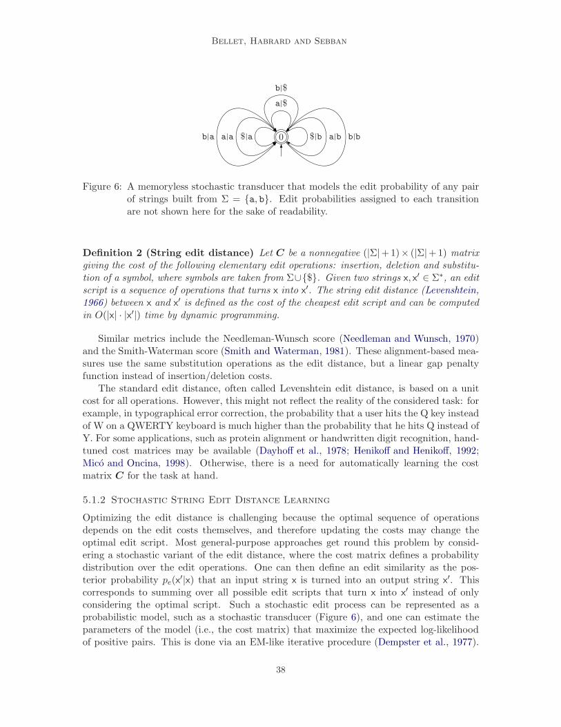
Bellet, Habrard and Sebban
Figure 6: A memoryless stochastic transducer that models the edit probability of any pairof strings built from Σ = a, b. Edit probabilities assigned to each transitionare not shown here for the sake of readability.
Definition 2 (String edit distance) Let C be a nonnegative (|Σ|+1)× (|Σ|+1) matrixgiving the cost of the following elementary edit operations: insertion, deletion and substitu-tion of a symbol, where symbols are taken from Σ∪$. Given two strings x, x′ ∈ Σ∗, an editscript is a sequence of operations that turns x into x
′. The string edit distance (Levenshtein,1966) between x and x
′ is defined as the cost of the cheapest edit script and can be computedin O(|x| · |x′|) time by dynamic programming.
Similar metrics include the Needleman-Wunsch score (Needleman and Wunsch, 1970)and the Smith-Waterman score (Smith and Waterman, 1981). These alignment-based mea-sures use the same substitution operations as the edit distance, but a linear gap penaltyfunction instead of insertion/deletion costs.
The standard edit distance, often called Levenshtein edit distance, is based on a unitcost for all operations. However, this might not reflect the reality of the considered task: forexample, in typographical error correction, the probability that a user hits the Q key insteadof W on a QWERTY keyboard is much higher than the probability that he hits Q instead ofY. For some applications, such as protein alignment or handwritten digit recognition, hand-tuned cost matrices may be available (Dayhoff et al., 1978; Henikoff and Henikoff, 1992;Mico and Oncina, 1998). Otherwise, there is a need for automatically learning the costmatrix C for the task at hand.
5.1.2 Stochastic String Edit Distance Learning
Optimizing the edit distance is challenging because the optimal sequence of operationsdepends on the edit costs themselves, and therefore updating the costs may change theoptimal edit script. Most general-purpose approaches get round this problem by consid-ering a stochastic variant of the edit distance, where the cost matrix defines a probabilitydistribution over the edit operations. One can then define an edit similarity as the pos-terior probability pe(x
′|x) that an input string x is turned into an output string x′. This
corresponds to summing over all possible edit scripts that turn x into x′ instead of only
considering the optimal script. Such a stochastic edit process can be represented as aprobabilistic model, such as a stochastic transducer (Figure 6), and one can estimate theparameters of the model (i.e., the cost matrix) that maximize the expected log-likelihoodof positive pairs. This is done via an EM-like iterative procedure (Dempster et al., 1977).
38
A Survey on Metric Learning for Feature Vectors and Structured Data
Note that unlike the standard edit distance, the obtained edit similarity does not usuallysatisfy the properties of a distance (in fact, it is often not symmetric and rarely satisfies thetriangular inequality).
Ristad and Yianilos The first method for learning a string edit metric, in the form ofa generative model, was proposed by Ristad and Yianilos (1998).46 They use a memory-less stochastic transducer which models the joint probability of a pair pe(x, x
′) from whichpe(x
′|x) can be estimated. Parameter estimation is performed with an EM procedure. TheExpectation step takes the form of a probabilistic version of the dynamic programing algo-rithm of the standard edit distance. The M-step aims at maximizing the likelihood of thetraining pairs of strings so as to define a joint distribution over the edit operations:
∑
(u,v)∈(Σ∪$)2\$,$
Cuv + c(#) = 1, with c(#) > 0 and Cuv ≥ 0,
where # is a termination symbol and c(#) the associated cost (probability).
Note that Bilenko and Mooney (2003) extended this approach to the Needleman-Wunschscore with affine gap penalty and applied it to duplicate detection. To deal with the ten-dency of Maximum Likelihood estimators to overfit when the number of parameters is large(in this case, when the alphabet size is large), Takasu (2009) proposes a Bayesian parameterestimation of pair-HMM providing a way to smooth the estimation.
Oncina and Sebban The work of Oncina and Sebban (2006) describes three levels ofbias induced by the use of generative models: (i) dependence between edit operations,(ii) dependence between the costs and the prior distribution of strings pe(x), and (iii) thefact that to obtain the posterior probability one must divide by the empirical estimate ofpe(x). These biases are highlighted by empirical experiments conducted with the methodof Ristad and Yianilos (1998). To address these limitations, they propose the use of a con-ditional transducer as a discriminative model that directly models the posterior probabilityp(x′|x) that an input string x is turned into an output string x
′ using edit operations.46
Parameter estimation is also done with EM where the maximization step differs from thatof Ristad and Yianilos (1998) as shown below:
∀u ∈ Σ,∑
v∈Σ∪$
Cv|u +∑
v∈Σ
Cv|$ = 1, with∑
v∈Σ
Cv|$ + c(#) = 1.
In order to allow the use of negative pairs, McCallum et al. (2005) consider anotherdiscriminative model, conditional random fields, that can deal with positive and negativepairs in specific states, still using EM for parameter estimation.
5.1.3 String Edit Distance Learning by Gradient Descent
The use of EM has two main drawbacks: (i) it may converge to a local optimum, and(ii) parameter estimation and distance calculations must be done at each iteration, whichcan be very costly if the size of the alphabet and/or the length of the strings are large.
46. An implementation is available within the SEDiL platform (Boyer et al., 2008):http://labh-curien.univ-st-etienne.fr/SEDiL/
39

Bellet, Habrard and Sebban
The following methods get round these drawbacks by formulating the learning problem inthe form of an optimization problem that can be efficiently solved by a gradient descentprocedure.
Saigo et al. Saigo et al. (2006) manage to avoid the need for an iterative procedurelike EM in the context of detecting remote homology in protein sequences.47 They learnthe parameters of the Smith-Waterman score which is plugged in their local alignmentkernel kLA where all the possible local alignments π for changing x into x
′ are taken intoaccount (Saigo et al., 2004):
kLA(x, x′) =
∑
π
et·s(x,x′,π). (19)
In the above formula, t is a parameter and s(x, x′, π) is the corresponding score of π anddefined as follows:
s(x, x′, π) =∑
u,v∈Σ
nu,v(x, x′, π) ·Cuv − ngd(x, x
′, π) · gd − nge(x, x′, π) · ge, (20)
where nu,v(x, x′, π) is the number of times that symbol u is aligned with v while gd and
ge, along with their corresponding number of occurrences ngd(x, x′, π) and nge(x, x
′, π), aretwo parameters dealing respectively with the opening and extension of gaps.
Unlike the Smith-Waterman score, kLA is differentiable and can be optimized by agradient descent procedure. The objective function that they optimize is meant to favorthe discrimination between positive and negative examples, but this is done by only usingpositive pairs of distant homologs. The approach has two additional drawbacks: (i) theobjective function is nonconvex and thus subject to local minima, and (ii) in general, kLAdoes not fulfill the properties of a kernel.
GESL (Bellet et al.) Bellet et al. (2011, 2012a) propose a convex programming ap-proach to learn edit similarity functions from both positive and negative pairs withoutrequiring a costly iterative procedure.48 They use the following simplified edit function:
eC(x, x′) =∑
(u,v)∈(Σ∪$)2\$,$
Cuv ·#uv(x, x′),
where #uv(x, x′) is the number of times the operation u → v appears in the Levenshtein
script. Therefore, eC can be optimized directly since the sequence of operations is fixed (itdoes not depend on the costs). The authors optimize the nonlinear similarity KC(x, x′) =2 exp(−eC(x, x′)) − 1, derived from eC . Note that KC is not required to be PSD norsymmetric. GESL (Good Edit Similarity Learning) is expressed as follows:
minC,B1,B2
1
n2
∑
zi,zj
ℓ(C, zi, zj) + β‖C‖2F
s.t. B1 ≥ − log(1
2), 0 ≤ B2 ≤ − log(
1
2), B1 −B2 = ηγ ,
47. Source code available at: http://sunflower.kuicr.kyoto-u.ac.jp/~hiroto/project/optaa.html48. Source code available at: http://www-bcf.usc.edu/~bellet/
40

A Survey on Metric Learning for Feature Vectors and Structured Data
where β ≥ 0 is a regularization parameter, ηγ ≥ 0 a parameter corresponding to a desired“margin” and
ℓ(C, zi, zj) =
[B1− eC(xi, xj)]+ if yi 6= yj[eC(xi, xj)−B2]+ if yi = yj.
GESL essentially learns the edit cost matrix C so as to optimize the (ǫ, γ, τ)-goodness(Balcan et al., 2008a) of the similarity KC(x, x′) and thereby enjoys generalization guaran-tees both for the learned similarity and for the resulting linear classifier (see Section 4.5).A potential drawback of GESL is that it optimized a simplified variant of the edit dis-tance, although this does not seem to be an issue in practice. Note that GESL can bestraightforwardly adapted to learn tree or graph edit similarities (Bellet et al., 2012a).
5.2 Tree and Graph Edit Distance Learning
In this section, we briefly review the main approaches in tree/graph edit distance learning.We do not delve into the details of these approaches as they are essentially adaptations ofstochastic string edit distance learning presented in Section 5.1.2.
Bernard et al. Extending the work of Ristad and Yianilos (1998) and Oncina and Sebban(2006) on string edit similarity learning, Bernard et al. (2006, 2008) propose both a gener-ative and a discriminative model for learning tree edit costs.46 They rely on the tree editdistance by Selkow (1977)—which is cheaper to compute than that of Zhang and Shasha(1989)—and adapt the updates of EM to this case.
Boyer et al. The work of Boyer et al. (2007) tackles the more complex variant of the treeedit distance (Zhang and Shasha, 1989), which allows the insertion and deletion of singlenodes instead of entire subtrees only.46 Parameter estimation in the generative model isalso based on EM.
Dalvi et al. The work of Dalvi et al. (2009) points out a limitation of the approach ofBernard et al. (2006, 2008): they model a distribution over tree edit scripts rather than overthe trees themselves, and unlike the case of strings, there is no bijection between the editscripts and the trees. Recovering the correct conditional probability with respect to treesrequires a careful and costly procedure. They propose a more complex conditional trans-ducer that models the conditional probability over trees and use again EM for parameterestimation.
Emms The work of Emms (2012) points out a theoretical limitation of the approachof Boyer et al. (2007): the authors use a factorization that turns out to be incorrect insome cases. Emms shows that a correct factorization exists when only considering the editscript of highest probability instead of all possible scripts, and derives the correspondingEM updates. An obvious drawback is that the output of the model is not the probabilityp(x′|x). Moreover, the approach is prone to overfitting and requires smoothing and otherheuristics (such as a final step of zeroing-out the diagonal of the cost matrix).
Neuhaus & Bunke In their paper, Neuhaus and Bunke (2007) learn a (more general)graph edit similarity, where each edit operation is modeled by a Gaussian mixture density.Parameter estimation is done using an EM-like algorithm. Unfortunately, the approach is
41

Bellet, Habrard and Sebban
intractable: the complexity of the EM procedure is exponential in the number of nodes (andso is the computation of the distance).
6. Conclusion and Discussion
In this survey, we provided a comprehensive review of the main methods and trends inmetric learning. We here briefly summarize and draw promising lines for future research.
6.1 Summary
Numerical data While metric learning for feature vectors was still in its early life at thetime of the first survey (Yang and Jin, 2006), it has now reached a good maturity level.Indeed, recent methods are able to deal with a large spectrum of settings in a scalable way.In particular, online approaches have played a significant role towards better scalability,complex tasks can be tackled through nonlinear or local metric learning, methods have beenderived for difficult settings such as ranking, multi-task learning or domain adaptation, andthe question of generalization in metric learning has been the focus of recent papers.
Structured data On the other hand, much less work has gone into metric learning forstructured data and advances made for numerical data have not yet propagated to structureddata. Indeed, most approaches remain based on EM-like algorithms which make themintractable for large datasets and instance size, and hard to analyze due to local optima.Nevertheless, recent advances such as GESL (Bellet et al., 2011) have shown that drawinginspiration from successful feature vector formulations (even if it requires simplifying themetric) can be highly beneficial in terms of scalability and flexibility. This is promisingdirection and probably a good omen for the development of this research area.
6.2 What next?
In light of this survey, we can identify the limitations of the current literature and speculateon where the future of metric learning is going.
Scalability with both n and d There has been satisfying solutions to perform metriclearning on large datasets (“Big Data”) through online learning or stochastic optimization.The question of scalability with the dimensionality is more involved, since most methodslearn O(d2) parameters, which is intractable for real-world applications involving thousandsof features, unless dimensionality reduction is applied beforehand. Kernelized methodshave O(n2) parameters instead, but this is infeasible when n is also large. Therefore, thechallenge of achieving high scalability with both n and d has yet to be overcome. Recentapproaches have tackled the problem by optimizing over the manifold of low-rank matrices(Shalit et al., 2012; Cheng, 2013) or defining the metric based on a combination of simpleclassifiers (Kedem et al., 2012; Xiong et al., 2012). These approaches have a good potentialfor future research.
More theoretical understanding Although several recent papers have looked at thegeneralization of metric learning, analyzing the link between the consistency of the learnedmetric and its performance in a given algorithm (classifier, clustering procedure, etc) re-mains an important open problem. So far, only results for linear classification have been
42

A Survey on Metric Learning for Feature Vectors and Structured Data
obtained (Bellet et al., 2012b; Guo and Ying, 2014), while learned metrics are also heavilyused for k-NN classification, clustering or information retrieval, for which no theoreticalresult is known.
Unsupervised metric learning A natural question to ask is whether one can learn ametric in a purely unsupervised way. So far, this has only been done as a byproduct ofdimensionality reduction algorithms. Other relevant criteria should be investigated, forinstance learning a metric that is robust to noise or invariant to some transformations ofinterest, in the spirit of denoising autoencoders (Vincent et al., 2008; Chen et al., 2012).Some results in this direction have been obtained for image transformations (Kumar et al.,2007). A related problem is to characterize what it means for a metric to be good for cluster-ing. There has been preliminary work on this question (Balcan et al., 2008b; Lajugie et al.,2014), which deserves more attention.
Leveraging the structure The simple example of metric learning designed specificallyfor histogram data (Kedem et al., 2012) has shown that taking the structure of the datainto account when learning the metric can lead to significant improvements in performance.As data is becoming more and more structured (e.g., social networks), using this structureto bias the choice of metric is likely to receive increasing interest in the near future.
Adapting the metric to changing data An important issue is to develop methodsrobust to changes in the data. In this line of work, metric learning in the presence ofnoisy data as well as for transfer learning and domain adaptation have recently receivedsome interest. However, these efforts are still insufficient for dealing with lifelong learningapplications, where the learner experiences concept drift and must detect and adapt themetric to different changes.
Learning richer metrics Existing metric learning algorithms ignore the fact that thenotion of similarity is often multimodal: there exist several ways in which two instances maybe similar (perhaps based on different features), and different degrees of similarity (versusthe simple binary similar/dissimilar view). Being able to model these shades as well as tointerpret why things are similar would bring the learned metrics closer to our own notionsof similarity.
Acknowledgments
We would like to acknowledge support from the ANR LAMPADA 09-EMER-007-02 project.
References
M. Ehsan Abbasnejad, Dhanesh Ramachandram, and Mandava Rajeswari. A survey of thestate of the art in learning the kernels. Knowledge and Information Systems (KAIS), 31(2):193–221, 2012.
Pierre-Antoine Absil, Robert Mahony, and Rodolphe Sepulchre. Optimization Algorithmson Matrix Manifolds. Princeton University Press, 2008.
43

Bellet, Habrard and Sebban
Ricardo Baeza-Yates and Berthier Ribeiro-Neto. Modern Information Retrieval. Addison-Wesley, 1999.
Mahdieh S. Baghshah and Saeed B. Shouraki. Semi-Supervised Metric Learning Using Pair-wise Constraints. In Proceedings of the 20th International Joint Conference on ArtificialIntelligence (IJCAI), pages 1217–1222, 2009.
Maria-Florina Balcan, Avrim Blum, and Nathan Srebro. Improved Guarantees for Learningvia Similarity Functions. In Proceedings of the 21st Annual Conference on LearningTheory (COLT), pages 287–298, 2008a.
Maria-Florina Balcan, Avrim Blum, and Santosh Vempala. A Discriminative Frameworkfor Clustering via Similarity Functions. In ACM Symposium on Theory of Computing(STOC), pages 671–680, 2008b.
Aharon Bar-Hillel, Tomer Hertz, Noam Shental, and Daphna Weinshall. Learning Dis-tance Functions using Equivalence Relations. In Proceedings of the 20th InternationalConference on Machine Learning (ICML), pages 11–18, 2003.
Aharon Bar-Hillel, Tomer Hertz, Noam Shental, and Daphna Weinshall. Learning a Ma-halanobis Metric from Equivalence Constraints. Journal of Machine Learning Research(JMLR), 6:937–965, 2005.
Peter L. Bartlett and Shahar Mendelson. Rademacher and Gaussian Complexities: RiskBounds and Structural Results. Journal of Machine Learning Research (JMLR), 3:463–482, 2002.
Jonathan Baxter and Peter L. Bartlett. The Canonical Distortion Measure in Feature Spaceand 1-NN Classification. In Advances in Neural Information Processing Systems (NIPS)10, 1997.
Mikhail Belkin and Partha Niyogi. Semi-Supervised Learning on Riemannian Manifolds.Machine Learning Journal (MLJ), 56(1–3):209–239, 2004.
Aurelien Bellet. Supervised Metric Learning with Generalization Guarantees. PhD thesis,University of Saint-Etienne, 2012.
Aurelien Bellet and Amaury Habrard. Robustness and Generalization for Metric Learning.Technical report, University of Saint-Etienne, September 2012. arXiv:1209.1086.
Aurelien Bellet, Amaury Habrard, and Marc Sebban. Learning Good Edit Similarities withGeneralization Guarantees. In Proceedings of the European Conference on Machine Learn-ing and Principles and Practice of Knowledge Discovery in Databases (ECML/PKDD),pages 188–203, 2011.
Aurelien Bellet, Amaury Habrard, and Marc Sebban. Good edit similarity learning by lossminimization. Machine Learning Journal (MLJ), 89(1):5–35, 2012a.
Aurelien Bellet, Amaury Habrard, and Marc Sebban. Similarity Learning for ProvablyAccurate Sparse Linear Classification. In Proceedings of the 29th International Conferenceon Machine Learning (ICML), pages 1871–1878, 2012b.
44

A Survey on Metric Learning for Feature Vectors and Structured Data
Xianye Ben, Weixiao Meng, Rui Yan, and Kejun Wang. An improved biometrics techniquebased on metric learning approach. Neurocomputing, 97:44–51, 2012.
Shai Ben-David, John Blitzer, Koby Crammer, Alex Kulesza, Fernando Pereira, and Jen-nifer Wortman Vaughan. A theory of learning from different domains. Machine LearningJournal (MLJ), 79(1-2):151–175, 2010.
Aharon Ben-Tal, Laurent El Ghaoui, and Arkadi Nemirovski. Robust Optimization. Prince-ton University Press, 2009.
Marc Bernard, Amaury Habrard, and Marc Sebban. Learning Stochastic Tree Edit Dis-tance. In Proceedings of the 17th European Conference on Machine Learning (ECML),pages 42–53, 2006.
Marc Bernard, Laurent Boyer, Amaury Habrard, and Marc Sebban. Learning probabilisticmodels of tree edit distance. Pattern Recognition (PR), 41(8):2611–2629, 2008.
Jinbo Bi, Dijia Wu, Le Lu, Meizhu Liu, Yimo Tao, and Matthias Wolf. AdaBoost onlow-rank PSD matrices for metric learning. In Proceedings of the IEEE Conference onComputer Vision and Pattern Recognition (CVPR), pages 2617–2624, 2011.
Wei Bian. Constrained Empirical Risk Minimization Framework for Distance Metric Learn-ing. IEEE Transactions on Neural Networks and Learning Systems (TNNLS), 23(8):1194–1205, 2012.
Wei Bian and Dacheng Tao. Learning a Distance Metric by Empirical Loss Minimization. InProceedings of the 22nd International Joint Conference on Artificial Intelligence (IJCAI),pages 1186–1191, 2011.
Mikhail Bilenko and Raymond J. Mooney. Adaptive Duplicate Detection Using Learn-able String Similarity Measures. In Proceedings of the 9th ACM SIGKDD InternationalConference on Knowledge Discovery and Data Mining, pages 39–48, 2003.
Mikhail Bilenko, Sugato Basu, and Raymond J. Mooney. Integrating Constraints and Met-ric Learning in Semi-Supervised Clustering. In Proceedings of the 21st InternationalConference on Machine Learning (ICML), pages 81–88, 2004.
Philip Bille. A survey on tree edit distance and related problems. Theoretical ComputerScience (TCS), 337(1-3):217–239, 2005.
Olivier Bousquet and Andre Elisseeff. Stability and Generalization. Journal of MachineLearning Research (JMLR), 2:499–526, 2002.
Stephen Boyd and Lieven Vandenberghe. Convex Optimization. Cambridge UniversityPress, 2004.
Laurent Boyer, Amaury Habrard, and Marc Sebban. Learning Metrics between Tree Struc-tured Data: Application to Image Recognition. In Proceedings of the 18th EuropeanConference on Machine Learning (ECML), pages 54–66, 2007.
45

Bellet, Habrard and Sebban
Laurent Boyer, Yann Esposito, Amaury Habrard, Jose Oncina, and Marc Seb-ban. SEDiL: Software for Edit Distance Learning. In Proceedings of the Eu-ropean Conference on Machine Learning and Principles and Practice of Knowl-edge Discovery in Databases (ECML/PKDD), pages 672–677, 2008. URLhttp://labh-curien.univ-st-etienne.fr/SEDiL/.
Lev M. Bregman. The relaxation method of finding the common points of convex sets andits application to the solution of problems in convex programming. USSR ComputationalMathematics and Mathematical Physics, 7(3):200–217, 1967.
Bin Cao, Xiaochuan Ni, Jian-Tao Sun, Gang Wang, and Qiang Yang. Distance MetricLearning under Covariate Shift. In Proceedings of the 22nd International Joint Conferenceon Artificial Intelligence (IJCAI), pages 1204–1210, 2011.
Qiong Cao, Zheng-Chu Guo, and Yiming Ying. Generalization Bounds for Metric andSimilarity Learning. Technical report, University of Exeter, July 2012a. arXiv:1207.5437.
Qiong Cao, Yiming Ying, and Peng Li. Distance Metric Learning Revisited. In Proceed-ings of the European Conference on Machine Learning and Principles and Practice ofKnowledge Discovery in Databases (ECML/PKDD), pages 283–298, 2012b.
Rich Caruana. Multitask Learning. Machine Learning Journal (MLJ), 28(1):41–75, 1997.
Nicolo Cesa-Bianchi and Claudio Gentile. Improved Risk Tail Bounds for On-Line Algo-rithms. IEEE Transactions on Information Theory (TIT), 54(1):386–390, 2008.
Ratthachat Chatpatanasiri, Teesid Korsrilabutr, Pasakorn Tangchanachaianan, and Boon-serm Kijsirikul. A new kernelization framework for Mahalanobis distance learning algo-rithms. Neurocomputing, 73:1570–1579, 2010.
Gal Chechik, Uri Shalit, Varun Sharma, and Samy Bengio. An Online Algorithm for LargeScale Image Similarity Learning. In Advances in Neural Information Processing Systems(NIPS) 22, pages 306–314, 2009.
Gal Chechik, Varun Sharma, Uri Shalit, and Samy Bengio. Large Scale Online Learning ofImage Similarity Through Ranking. Journal of Machine Learning Research (JMLR), 11:1109–1135, 2010.
Minmin Chen, Zhixiang Eddie Xu, Kilian Q. Weinberger, and Fei Sha. Marginalized De-noising Autoencoders for Domain Adaptation. In Proceedings of the 29th InternationalConference on Machine Learning (ICML), 2012.
Li Cheng. Riemannian Similarity Learning. In Proceedings of the 30th International Con-ference on Machine Learning (ICML), 2013.
Sumit Chopra, Raia Hadsell, and Yann LeCun. Learning a Similarity Metric Discrimina-tively, with Application to Face Verification. In Proceedings of the IEEE Conference onComputer Vision and Pattern Recognition (CVPR), pages 539–546, 2005.
46

A Survey on Metric Learning for Feature Vectors and Structured Data
Corinna Cortes and Vladimir Vapnik. Support-Vector Networks. Machine Learning Journal(MLJ), 20(3):273–297, 1995.
Thomas Cover and Peter Hart. Nearest neighbor pattern classification. IEEE Transactionson Information Theory (TIT), 13(1):21–27, 1967.
Koby Crammer and Gal Chechik. Adaptive Regularization for Weight Matrices. In Pro-ceedings of the 29th International Conference on Machine Learning (ICML), 2012.
Koby Crammer, Ofer Dekel, Joseph Keshet, Shai Shalev-Shwartz, and Yoram Singer. OnlinePassive-Aggressive Algorithms. Journal of Machine Learning Research (JMLR), 7:551–585, 2006.
Marco Cuturi and David Avis. Ground Metric Learning. Technical report, Kyoto University,2011. 1110.2306.
Nilesh N. Dalvi, Philip Bohannon, and Fei Sha. Robust web extraction: an approach basedon a probabilistic tree-edit model. In Proceedings of the ACM SIGMOD InternationalConference on Management of data (COMAD), pages 335–348, 2009.
Jason V. Davis, Brian Kulis, Prateek Jain, Suvrit Sra, and Inderjit S. Dhillon. Information-theoretic metric learning. In Proceedings of the 24th International Conference on MachineLearning (ICML), pages 209–216, 2007.
Margaret O. Dayhoff, Robert M. Schwartz, and Bruce C. Orcutt. A model of evolutionarychange in proteins. Atlas of protein sequence and structure, 5(3):345–351, 1978.
Arthur P. Dempster, Nan M. Laird, and Donald B. Rubin. Maximum likelihood fromincomplete data via the EM algorithm. Journal of the Royal Statistical Society, SeriesB, 39(1):1–38, 1977.
Jia Deng, Alexander C. Berg, and Li Fei-Fei. Hierarchical semantic indexing for large scaleimage retrieval. In Proceedings of the IEEE Conference on Computer Vision and PatternRecognition (CVPR), pages 785–792, 2011.
Matthew Der and Lawrence K. Saul. Latent Coincidence Analysis: A Hidden VariableModel for Distance Metric Learning. In Advances in Neural Information ProcessingSystems (NIPS) 25, pages 3239–3247, 2012.
Inderjit S. Dhillon and Joel A. Tropp. Matrix Nearness Problems with Bregman Diver-gences. SIAM Journal on Matrix Analysis and Applications, 29(4):1120–1146, 2007.
Huyen Do, Alexandros Kalousis, Jun Wang, and Adam Woznica. A metric learning perspec-tive of SVM: on the relation of LMNN and SVM. In Proceedings of the 15th InternationalConference on Artificial Intelligence and Statistics (AISTATS), pages 308–317, 2012.
John Duchi, Shai Shalev-Shwartz, Yoram Singer, and Ambuj Tewari. Composite Objec-tive Mirror Descent. In Proceedings of the 23rd Annual Conference on Learning Theory(COLT), pages 14–26, 2010.
47

Bellet, Habrard and Sebban
Martin Emms. On Stochastic Tree Distances and Their Training via Expectation-Maximisation. In Proceedings of the 1st International Conference on Pattern RecognitionApplications and Methods (ICPRAM), pages 144–153, 2012.
Theodoros Evgeniou and Massimiliano Pontil. Regularized multi-task learning. In Proceed-ings of the 10th ACM SIGKDD International Conference on Knowledge Discovery andData Mining, pages 109–117, 2004.
Maryam Fazel, Haitham Hindi, and Stephen P. Boyd. A Rank Minimization Heuristic withApplication to Minimum Order System Approximation. In Proceedings of the AmericanControl Conference, pages 4734–4739, 2001.
Imola K. Fodor. A Survey of Dimension Reduction Techniques. Technical report, LawrenceLivermore National Laboratory, 2002. UCRL-ID- 148494.
Yoav Freund and Robert E. Schapire. A Decision-Theoretic Generalization of On-LineLearning and an Application to Boosting. In Proceedings of the 2nd European Conferenceon Computational Learning Theory (EuroCOLT), pages 23–37, 1995.
Jerome H. Friedman. Flexible Metric Nearest Neighbor Classification. Technical report,Department of Statistics, Stanford University, 1994.
Jerome H. Friedman. Greedy Function Approximation: A Gradient Boosting Machine.Annals of Statistics (AOS), 29(5):1189–1232, 2001.
Andrea Frome, Yoram Singer, Fei Sha, and Jitendra Malik. Learning Globally-ConsistentLocal Distance Functions for Shape-Based Image Retrieval and Classification. In Pro-ceedings of the IEEE International Conference on Computer Vision (ICCV), pages 1–8,2007.
Keinosuke Fukunaga. Introduction to Statistical Pattern Recognition. Academic Press, 1990.
Xinbo Gao, Bing Xiao, Dacheng Tao, and Xuelong Li. A survey of graph edit distance.Pattern Analysis and Applications (PAA), 13(1):113–129, 2010.
Bo Geng, Dacheng Tao, and Chao Xu. DAML: Domain Adaptation Metric Learning. IEEETransactions on Image Processing (TIP), 20(10):2980–2989, 2011.
Amir Globerson and Sam T. Roweis. Metric Learning by Collapsing Classes. In Advancesin Neural Information Processing Systems (NIPS) 18, pages 451–458, 2005.
Jacob Goldberger, Sam Roweis, Geoff Hinton, and Ruslan Salakhutdinov. NeighbourhoodComponents Analysis. In Advances in Neural Information Processing Systems (NIPS)17, pages 513–520, 2004.
Mehmet Gonen and Ethem Alpaydin. Multiple Kernel Learning Algorithms. Journal ofMachine Learning Research (JMLR), 12:2211–2268, 2011.
Yves Grandvalet and Yoshua Bengio. Semi-supervised Learning by Entropy Minimization.In Advances in Neural Information Processing Systems (NIPS) 17, pages 29–536, 2004.
48

A Survey on Metric Learning for Feature Vectors and Structured Data
Arthur Gretton, Karsten M. Borgwardt, Malte J. Rasch, Bernhard Scholkopf, and Alexan-der J. Smola. A Kernel Method for the Two-Sample-Problem. In Advances in NeuralInformation Processing Systems (NIPS) 19, pages 513–520, 2006.
Matthieu Guillaumin, Thomas Mensink, Jakob J. Verbeek, and Cordelia Schmid. TagProp:Discriminative metric learning in nearest neighbor models for image auto-annotation. InProceddings of the IEEE International Conference on Computer Vision (ICCV), pages309–316, 2009a.
Matthieu Guillaumin, Jakob J. Verbeek, and Cordelia Schmid. Is that you? Metric learningapproaches for face identification. In Proceddings of the IEEE International Conferenceon Computer Vision (ICCV), pages 498–505, 2009b.
Zheng-Chu Guo and Yiming Ying. Guaranteed Classification via Regularized SimilarityLearning. Neural Computation, 26(3):497–522, 2014.
James L. Hafner, Harpreet S. Sawhney, William Equitz, Myron Flickner, and WayneNiblack. Efficient Color Histogram Indexing for Quadratic Form Distance Functions.IEEE Transactions on Pattern Analysis and Machine Intelligence (TPAMI), 17(7):729–736, 1995.
Trevor Hastie and Robert Tibshirani. Discriminant Adaptive Nearest Neighbor Classifica-tion. IEEE Transactions on Pattern Analysis and Machine Intelligence (TPAMI), 18(6):607–616, 1996.
Søren Hauberg, Oren Freifeld, and Michael J. Black. A Geometric take on Metric Learning.In Advances in Neural Information Processing Systems (NIPS) 25, pages 2033–2041,2012.
Yujie He, Wenlin Chen, and Yixin Chen. Kernel Density Metric Learning. Technical report,Washington University in St. Louis, 2013.
Steven Henikoff and Jorja G. Henikoff. Amino acid substitution matrices from proteinblocks. Proceedings of the National Academy of Sciences of the United States of America,89(22):10915–10919, 1992.
Steven C. Hoi, Wei Liu, Michael R. Lyu, and Wei-Ying Ma. Learning Distance Metricswith Contextual Constraints for Image Retrieval. In Proceedings of the IEEE Conferenceon Computer Vision and Pattern Recognition (CVPR), pages 2072–2078, 2006.
Steven C. Hoi, Wei Liu, and Shih-Fu Chang. Semi-supervised distance metric learningfor Collaborative Image Retrieval. In Proceedings of the IEEE Conference on ComputerVision and Pattern Recognition (CVPR), 2008.
Steven C. Hoi, Wei Liu, and Shih-Fu Chang. Semi-supervised distance metric learning forcollaborative image retrieval and clustering. ACM Transactions on Multimedia Comput-ing, Communications, and Applications (TOMCCAP), 6(3), 2010.
49

Bellet, Habrard and Sebban
Yi Hong, Quannan Li, Jiayan Jiang, and Zhuowen Tu. Learning a mixture of sparse dis-tance metrics for classification and dimensionality reduction. In Proceedings of the IEEEInternational Conference on Computer Vision (ICCV), pages 906–913, 2011.
Kaizhu Huang, Yiming Ying, and Colin Campbell. GSML: A Unified Framework for SparseMetric Learning. In Proceedings of the IEEE International Conference on Data Mining(ICDM), pages 189–198, 2009.
Kaizhu Huang, Rong Jin, Zenglin Xu, and Cheng-Lin Liu. Robust Metric Learning bySmooth Optimization. In Proceedings of the 26th Conference on Uncertainty in ArtificialIntelligence (UAI), pages 244–251, 2010.
Kaizhu Huang, Yiming Ying, and Colin Campbell. Generalized sparse metric learning withrelative comparisons. Knowledge and Information Systems (KAIS), 28(1):25–45, 2011.
Yinjie Huang, Cong Li, Michael Georgiopoulos, and Georgios C. Anagnostopoulos.Reduced-Rank Local Distance Metric Learning. In Proceedings of the European Con-ference on Machine Learning and Principles and Practice of Knowledge Discovery inDatabases (ECML/PKDD), pages 224–239, 2013.
Prateek Jain, Brian Kulis, Inderjit S. Dhillon, and Kristen Grauman. Online Metric Learn-ing and Fast Similarity Search. In Advances in Neural Information Processing Systems(NIPS) 21, pages 761–768, 2008.
Prateek Jain, Brian Kulis, and Inderjit S. Dhillon. Inductive Regularized Learning of KernelFunctions. In Advances in Neural Information Processing Systems (NIPS) 23, pages 946–954, 2010.
Prateek Jain, Brian Kulis, Jason V. Davis, and Inderjit S. Dhillon. Metric and KernelLearning Using a Linear Transformation. Journal of Machine Learning Research (JMLR),13:519–547, 2012.
Nan Jiang, Wenyu Liu, and Ying Wu. Order determination and sparsity-regularized metriclearning adaptive visual tracking. In Proceedings of the IEEE Conference on ComputerVision and Pattern Recognition (CVPR), pages 1956–1963, 2012.
Rong Jin, Shijun Wang, and Yang Zhou. Regularized Distance Metric Learning: Theoryand Algorithm. In Advances in Neural Information Processing Systems (NIPS) 22, pages862–870, 2009.
Thorsten Joachims, Thomas Finley, and Chun-Nam J. Yu. Cutting-plane training of struc-tural SVMs. Machine Learning Journal (MLJ), 77(1):27–59, 2009.
Purushottam Kar, Bharath Sriperumbudur Prateek Jain, and Harish Karnick. On theGeneralization Ability of Online Learning Algorithms for Pairwise Loss Functions. InProceedings of the 30th International Conference on Machine Learning, 2013.
Tsuyoshi Kato and Nozomi Nagano. Metric learning for enzyme active-site search. Bioin-formatics, 26(21):2698–2704, 2010.
50

A Survey on Metric Learning for Feature Vectors and Structured Data
Dor Kedem, Stephen Tyree, Kilian Weinberger, Fei Sha, and Gert Lanckriet. Non-linearMetric Learning. In Advances in Neural Information Processing Systems (NIPS) 25,pages 2582–2590, 2012.
Brian Kulis. Metric Learning: A Survey. Foundations and Trends in Machine Learning(FTML), 5(4):287–364, 2012.
Brian Kulis, Prateek Jain, and Kristen Grauman. Fast Similarity Search for Learned Met-rics. IEEE Transactions on Pattern Analysis and Machine Intelligence (TPAMI), 31(12):2143–2157, 2009.
Brian Kulis, Kate Saenko, and Trevor Darrell. What you saw is not what you get: Domainadaptation using asymmetric kernel transforms. In Proceedings of the IEEE Conferenceon Computer Vision and Pattern Recognition (CVPR), pages 1785–1792, 2011.
Solomon Kullback and Richard Leibler. On Information and Sufficiency. Annals of Mathe-matical Statistics, 22(1):79–86, 1951.
M. Pawan Kumar, Philip H. S. Torr, and Andrew Zisserman. An Invariant Large MarginNearest Neighbour Classifier. In Proceedings of the IEEE International Conference onComputer Vision (ICCV), pages 1–8, 2007.
Gautam Kunapuli and Jude Shavlik. Mirror Descent for Metric Learning: A Unified Ap-proach. In Proceedings of the European Conference on Machine Learning and Principlesand Practice of Knowledge Discovery in Database (ECML/PKDD), pages 859–874, 2012.
Remi Lajugie, Sylvain Arlot, and Francis Bach. Large-Margin Metric Learning for Con-strained Partitioning Problems. In Proceedings of the 31st International Conference onMachine Learning (ICML), 2014.
Marc T. Law, Carlos S. Gutierrez, Nicolas Thome, and Stephane Gancarski. Structural andvisual similarity learning for Web page archiving. In Proceedings of the 10th InternationalWorkshop on Content-Based Multimedia Indexing (CBMI), pages 1–6, 2012.
Guy Lebanon. Metric Learning for Text Documents. IEEE Transactions on Pattern Anal-ysis and Machine Intelligence (TPAMI), 28(4):497–508, 2006.
Jung-Eun Lee, Rong Jin, and Anil K. Jain. Rank-based distance metric learning: Anapplication to image retrieval. In Proceedings of the IEEE Conference on ComputerVision and Pattern Recognition (CVPR), 2008.
Vladimir I. Levenshtein. Binary codes capable of correcting deletions, insertions and rever-sals. Soviet Physics-Doklandy, 6:707–710, 1966.
Fei-Fei Li and Pietro Perona. A Bayesian Hierarchical Model for Learning Natural SceneCategories. In Proceedings of the IEEE Conference on Computer Vision and PatternRecognition, pages 524–531, 2005.
51
Bellet, Habrard and Sebban
Xi Li, Chunhua Shen, Qinfeng Shi, Anthony Dick, and Anton van den Hengel. Non-sparse Linear Representations for Visual Tracking with Online Reservoir Metric Learn-ing. In Proceedings of the IEEE Conference on Computer Vision and Pattern Recognition(CVPR), pages 1760–1767, 2012.
Zhaohui Liang, Gang Zhang, Li Jiang, and Wenbin Fu. Learning a Consistent PRO-Outcomes Metric through KCCA for an Efficacy Assessing Model of Acupuncture. Jour-nal of Chinese Medicine Research and Development (JCMRD), 1(3):79–88, 2012.
Daryl K. Lim, Brian McFee, and Gert Lanckriet. Robust Structural Metric Learning. InProceedings of the 30th International Conference on Machine Learning (ICML), 2013.
Nick Littlestone. Learning Quickly When Irrelevant Attributes Abound: A New Linear-Threshold Algorithm. Machine Learning Journal (MLJ), 2(4):285–318, 1988.
Meizhu Liu and Baba C. Vemuri. A Robust and Efficient Doubly Regularized MetricLearning Approach. In Proceedings of the 12th European Conference on Computer Vision(ECCV), pages 646–659, 2012.
Wei Liu, Shiqian Ma, Dacheng Tao, Jianzhuang Liu, and Peng Liu. Semi-Supervised SparseMetric Learning using Alternating Linearization Optimization. In Proceedings of the16th ACM SIGKDD International Conference on Knowledge Discovery and Data Mining,pages 1139–1148, 2010.
Stuart P. Lloyd. Least squares quantization in PCM. IEEE Transactions on InformationTheory (TIT), 28:129–137, 1982.
Huma Lodhi, Craig Saunders, John Shawe-Taylor, Nello Cristianini, and Chris Watkins.Text Classification using String Kernels. Journal of Machine Learning Research (JMLR),2:419–444, 2002.
Jiwen Lu, Junlin Hu, Xiuzhuang Zhou, Yuanyuan Shang, Yap-Peng Tan, and Gang Wang.Neighborhood repulsed metric learning for kinship verification. In Proceedings of theIEEE Conference on Computer Vision and Pattern Recognition (CVPR), pages 2594–2601, 2012.
Prasanta Chandra Mahalanobis. On the generalised distance in statistics. Proceedings ofthe National Institute of Sciences of India, 2(1):49–55, 1936.
Yishay Mansour, Mehryar Mohri, and Afshin Rostamizadeh. Domain Adaptation: LearningBounds and Algorithms. In Proceedings of the 22nd Annual Conference on LearningTheory (COLT), 2009.
Andrew McCallum, Kedar Bellare, and Fernando Pereira. A Conditional Random Fieldfor Discriminatively-trained Finite-state String Edit Distance. In Proceedings of the 21stConference in Uncertainty in Artificial Intelligence (UAI), pages 388–395, 2005.
Brian McFee and Gert R. G. Lanckriet. Metric Learning to Rank. In Proceedings of the27th International Conference on Machine Learning (ICML), pages 775–782, 2010.
52

A Survey on Metric Learning for Feature Vectors and Structured Data
Brian McFee, Luke Barrington, and Gert R. G. Lanckriet. Learning Content Similarity forMusic Recommendation. IEEE Transactions on Audio, Speech & Language Processing(TASLP), 20(8):2207–2218, 2012.
Thomas Mensink, Jakob J. Verbeek, Florent Perronnin, and Gabriela Csurka. Metric Learn-ing for Large Scale Image Classification: Generalizing to New Classes at Near-Zero Cost.In Proceedings of the 12th European Conference on Computer Vision (ECCV), pages488–501, 2012.
Luisa Mico and Jose Oncina. Comparison of fast nearest neighbour classifiers for handwrit-ten character recognition. Pattern Recognition Letters (PRL), 19:351–356, 1998.
Saul B. Needleman and Christian D. Wunsch. A general method applicable to the searchfor similarities in the amino acid sequence of two proteins. Journal of Molecular Biology(JMB), 48(3):443–453, 1970.
Yurii Nesterov. Smooth minimization of non-smooth functions. Mathematical Programming,103:127–152, 2005.
Michel Neuhaus and Horst Bunke. Automatic learning of cost functions for graph editdistance. Journal of Information Science (JIS), 177(1):239–247, 2007.
Behnam Neyshabur, Nati Srebro, Ruslan Salakhutdinov, Yury Makarychev, and PaymanYadollahpour. The Power of Asymmetry in Binary Hashing. In Advances in NeuralInformation Processing Systems (NIPS) 26, pages 2823–2831, 2013.
Hieu V. Nguyen and Li Bai. Cosine Similarity Metric Learning for Face Verification. InProceedings of the 10th Asian Conference on Computer Vision (ACCV), pages 709–720,2010.
Nam Nguyen and Yunsong Guo. Metric Learning: A Support Vector Approach. In Pro-ceedings of the European Conference on Machine Learning and Principles and Practiceof Knowledge Discovery in Databases (ECML/PKDD), pages 125–136, 2008.
Gang Niu, Bo Dai, Makoto Yamada, and Masashi Sugiyama. Information-theoretic Semi-supervised Metric Learning via Entropy Regularization. In Proceedings of the 29th Inter-national Conference on Machine Learning (ICML), 2012.
Yung-Kyun Noh, Byoung-Tak Zhang, and Daniel D. Lee. Generative Local Metric Learn-ing for Nearest Neighbor Classification. In Advances in Neural Information ProcessingSystems (NIPS) 23, pages 1822–1830, 2010.
Mohammad Norouzi, David J. Fleet, and Ruslan Salakhutdinov. Hamming Distance MetricLearning. In Advances in Neural Information Processing Systems (NIPS) 25, pages 1070–1078, 2012a.
Mohammad Norouzi, Ali Punjani, and David J. Fleet. Fast Search in Hamming Space withMulti-Index Hashing. In Proceedings of the IEEE Conference on Computer Vision andPattern Recognition (CVPR), 2012b.
53

Bellet, Habrard and Sebban
Jose Oncina and Marc Sebban. Learning Stochastic Edit Distance: application in hand-written character recognition. Pattern Recognition (PR), 39(9):1575–1587, 2006.
Shibin Parameswaran and Kilian Q. Weinberger. Large Margin Multi-Task Metric Learning.In Advances in Neural Information Processing Systems (NIPS) 23, pages 1867–1875,2010.
Kyoungup Park, Chunhua Shen, Zhihui Hao, and Junae Kim. Efficiently Learning a Dis-tance Metric for Large Margin Nearest Neighbor Classification. In Proceedings of the 25thAAAI Conference on Artificial Intelligence, 2011.
Karl Pearson. On Lines and Planes of Closest Fit to Points in Space. Philosophical Magazine,2(6):559–572, 1901.
Ali M. Qamar and Eric Gaussier. Online and Batch Learning of Generalized Cosine Simi-larities. In Proceedings of the IEEE International Conference on Data Mining (ICDM),pages 926–931, 2009.
Ali M. Qamar and Eric Gaussier. RELIEF Algorithm and Similarity Learning for k-NN.International Journal of Computer Information Systems and Industrial Management Ap-plications (IJCISIM), 4:445–458, 2012.
Ali M. Qamar, Eric Gaussier, Jean-Pierre Chevallet, and Joo-Hwee Lim. Similarity Learningfor Nearest Neighbor Classification. In Proceedings of the IEEE International Conferenceon Data Mining (ICDM), pages 983–988, 2008.
Guo-Jun Qi, Jinhui Tang, Zheng-Jun Zha, Tat-Seng Chua, and Hong-Jiang Zhang.An Efficient Sparse Metric Learning in High-Dimensional Space via l1-Penalized Log-Determinant Regularization. In Proceedings of the 26th International Conference onMachine Learning (ICML), 2009.
Qi Qian, Rong Jin, Jinfeng Yi, Lijun Zhang, and Shenghuo Zhu. Efficient Distance MetricLearning by Adaptive Sampling and Mini-Batch Stochastic Gradient Descent (SGD).arXiv:1304.1192, April 2013.
Joaquin Quinonero-Candela. Dataset Shift in Machine Learning. MIT Press, 2009.
Deva Ramanan and Simon Baker. Local Distance Functions: A Taxonomy, New Algorithms,and an Evaluation. IEEE Transactions on Pattern Analysis and Machine Intelligence(TPAMI), 33(4):794–806, 2011.
Pradeep Ravikumar, Martin J. Wainwright, Garvesh Raskutti, and Bin Yu. High-dimensional covariance estimation by minimizing ℓ1-penalized log-determinant diver-gence. Electronic Journal of Statistics, 5:935–980, 2011.
Eric S. Ristad and Peter N. Yianilos. Learning String-Edit Distance. IEEE Transactionson Pattern Analysis and Machine Intelligence (TPAMI), 20(5):522–532, 1998.
Romer Rosales and Glenn Fung. Learning Sparse Metrics via Linear Programming. InProceedings of the 12th ACM SIGKDD International Conference on Knowledge Discoveryand Data Mining, pages 367–373, 2006.
54
A Survey on Metric Learning for Feature Vectors and Structured Data
Yossi Rubner, Carlo Tomasi, and Leonidas J. Guibas. The Earth Mover’s Distance as aMetric for Image Retrieval. International Journal of Computer Vision (IJCV), 40(2):99–121, 2000.
Kate Saenko, Brian Kulis, Mario Fritz, and Trevor Darrell. Adapting Visual CategoryModels to New Domains. In Proceedings of the 11th European Conference on ComputerVision (ECCV), pages 213–226, 2010.
Hiroto Saigo, Jean-Philippe Vert, Nobuhisa Ueda, and Tatsuya Akutsu. Protein homologydetection using string alignment kernels. Bioinformatics, 20(11):1682–1689, 2004.
Hiroto Saigo, Jean-Philippe Vert, and Tatsuya Akutsu. Optimizing amino acid substitutionmatrices with a local alignment kernel. Bioinformatics, 7(246):1–12, 2006.
Ruslan Salakhutdinov and Geoffrey E. Hinton. Learning a Nonlinear Embedding by Preserv-ing Class Neighbourhood Structure. In Proceedings of the 11th International Conferenceon Artificial Intelligence and Statistics (AISTATS), pages 412–419, 2007.
Gerard Salton, AndrewWong, and C. S. Yang. A vector space model for automatic indexing.Communications of the ACM, 18(11):613–620, 1975.
Robert E. Schapire and Yoav Freund. Boosting: Foundations and Algorithms. MIT Press,2012.
Bernhard Scholkopf, Alexander Smola, and Klaus-Robert Muller. Nonlinear componentanalysis as a kernel eigenvalue problem. Neural Computation (NECO), 10(1):1299–1319,1998.
Matthew Schultz and Thorsten Joachims. Learning a Distance Metric from Relative Com-parisons. In Advances in Neural Information Processing Systems (NIPS) 16, 2003.
Stanley M. Selkow. The tree-to-tree editing problem. Information Processing Letters, 6(6):184–186, 1977.
Shai Shalev-Shwartz, Yoram Singer, and Andrew Y. Ng. Online and batch learning ofpseudo-metrics. In Proceedings of the 21st International Conference on Machine Learning(ICML), 2004.
Uri Shalit, Daphna Weinshall, and Gal Chechik. Online Learning in The Manifold of Low-Rank Matrices. In Advances in Neural Information Processing Systems (NIPS) 23, pages2128–2136, 2010.
Uri Shalit, Daphna Weinshall, and Gal Chechik. Online Learning in the Embedded Manifoldof Low-rank Matrices. Journal of Machine Learning Research (JMLR), 13:429–458, 2012.
Blake Shaw, Bert C. Huang, and Tony Jebara. Learning a Distance Metric from a Network.In Advances in Neural Information Processing Systems (NIPS) 24, pages 1899–1907,2011.
55

Bellet, Habrard and Sebban
Chunhua Shen, Junae Kim, Lei Wang, and Anton van den Hengel. Positive SemidefiniteMetric Learning with Boosting. In Advances in Neural Information Processing Systems(NIPS) 22, pages 1651–1660, 2009.
Chunhua Shen, Junae Kim, Lei Wang, and Anton van den Hengel. Positive SemidefiniteMetric Learning Using Boosting-like Algorithms. Journal of Machine Learning Research(JMLR), 13:1007–1036, 2012.
Noam Shental, Tomer Hertz, Daphna Weinshall, and Misha Pavel. Adjustment Learningand Relevant Component Analysis. In Proceedings of the 7th European Conference onComputer Vision (ECCV), pages 776–792, 2002.
Yuan Shi, Yung-Kyun Noh, Fei Sha, and Daniel D. Lee. Learning Discriminative Metricsvia Generative Models and Kernel Learning. arXiv:1109.3940, September 2011.
Robert D. Short and Keinosuke Fukunaga. The optimal distance measure for nearest neigh-bor classification. IEEE Transactions on Information Theory (TIT), 27(5):622–626, 1981.
Josef Sivic and Andrew Zisserman. Efficient visual search of videos cast as text retrieval.IEEE Transactions on Pattern Analysis and Machine Intelligence (TPAMI), 31:591–606,2009.
Temple F. Smith and Michael S. Waterman. Identification of common molecular subse-quences. Journal of Molecular Biology (JMB), 147(1):195–197, 1981.
Atsuhiro Takasu. Bayesian Similarity Model Estimation for Approximate Recognized TextSearch. In Proceedings of the 10th International Conference on Document Analysis andRecognition (ICDAR), pages 611–615, 2009.
Daniel Tarlow, Kevin Swersky, Ilya Sutskever, Laurent Charlin, and Rich Zemel. Stochastick-Neighborhood Selection for Supervised and Unsupervised Learning. In Proceedings ofthe 30th International Conference on Machine Learning (ICML), 2013.
Matthew E. Taylor, Brian Kulis, and Fei Sha. Metric learning for reinforcement learningagents. In Proceedings of the 10th International Conference on Autonomous Agents andMultiagent Systems (AAMAS), pages 777–784, 2011.
Lorenzo Torresani and Kuang-Chih Lee. Large Margin Component Analysis. In Advancesin Neural Information Processing Systems (NIPS) 19, pages 1385–1392, 2006.
Ioannis Tsochantaridis, Thorsten Joachims, Thomas Hofmann, and Yasemin Altun. LargeMargin Methods for Structured and Interdependent Output Variables. Journal of Ma-chine Learning Research, 6:1453–1484, 2005.
Yuta Tsuboi, Hisashi Kashima, Shohei Hido, Steffen Bickel, and Masashi Sugiyama. DirectDensity Ratio Estimation for Large-scale Covariate Shift Adaptation. In Proceedings ofthe SIAM International Conference on Data Mining (SDM), pages 443–454, 2008.
Leslie G. Valiant. A theory of the learnable. Communications of the ACM, 27:1134–1142,1984.
56

A Survey on Metric Learning for Feature Vectors and Structured Data
Laurens J.P. van der Maaten, Eric O. Postma, and H. Jaap van den Herik. DimensionalityReduction: A Comparative Review. Technical report, Tilburg University, 2009. TiCC-TR2009-005.
Vladimir N. Vapnik and Alexey Y. Chervonenkis. On the uniform convergence of relativefrequencies of events to their probabilities. Theory of Probability and its Applications(TPA), 16(2):264–280, 1971.
Nakul Verma, Dhruv Mahajan, Sundararajan Sellamanickam, and Vinod Nair. LearningHierarchical Similarity Metrics. In Proceedings of the IEEE Conference on ComputerVision and Pattern Recognition (CVPR), pages 2280–2287, 2012.
Pascal Vincent, Hugo Larochelle, Yoshua Bengio, and Pierre-Antoine Manzagol. Extractingand composing robust features with denoising autoencoders. In Proceedings of the 25thInternational Conference on Machine Learning (ICML), pages 1096–1103, 2008.
Fan Wang and Leonidas J. Guibas. Supervised Earth Mover’s Distance Learning and ItsComputer Vision Applications. In Proceedings of the 12th European Conference on Com-puter Vision (ECCV), pages 442–455, 2012.
Jingyan Wang, Xin Gao, Quanquan Wang, and Yongping Li. ProDis-ContSHC: learn-ing protein dissimilarity measures and hierarchical context coherently for protein-proteincomparison in protein database retrieval. BMC Bioinformatics, 13(S-7):S2, 2012a.
Jun Wang, Huyen T. Do, Adam Woznica, and Alexandros Kalousis. Metric Learning withMultiple Kernels. In Advances in Neural Information Processing Systems (NIPS) 24,pages 1170–1178, 2011.
Jun Wang, Adam Woznica, and Alexandros Kalousis. Learning Neighborhoods for MetricLearning. In Proceedings of the European Conference on Machine Learning and Princi-ples and Practice of Knowledge Discovery in Databases (ECML/PKDD), pages 223–236,2012b.
Jun Wang, Adam Woznica, and Alexandros Kalousis. Parametric Local Metric Learning forNearest Neighbor Classification. In Advances in Neural Information Processing Systems(NIPS) 25, pages 1610–1618, 2012c.
Qianying Wang, Pong C. Yuen, and Guocan Feng. Semi-supervised metric learning viatopology preserving multiple semi-supervised assumptions. Pattern Recognition (PR),2013a.
Yuyang Wang, Roni Khardon, Dmitry Pechyony, and Rosie Jones. Generalization Boundsfor Online Learning Algorithms with Pairwise Loss Functions. In Proceedings of the 25thAnnual Conference on Learning Theory (COLT), pages 13.1–13.22, 2012d.
Yuyang Wang, Roni Khardon, Dmitry Pechyony, and Rosie Jones. Online Learningwith Pairwise Loss Functions. Technical report, Tufts University, January 2013b.arXiv:1301.5332.
57

Bellet, Habrard and Sebban
Kilian Q. Weinberger and Lawrence K. Saul. Fast Solvers and Efficient Implementationsfor Distance Metric Learning. In Proceedings of the 25th International Conference onMachine Learning (ICML), pages 1160–1167, 2008.
Kilian Q. Weinberger and Lawrence K. Saul. Distance Metric Learning for Large MarginNearest Neighbor Classification. Journal of Machine Learning Research (JMLR), 10:207–244, 2009.
Kilian Q. Weinberger, John Blitzer, and Lawrence K. Saul. Distance Metric Learningfor Large Margin Nearest Neighbor Classification. In Advances in Neural InformationProcessing Systems (NIPS) 18, pages 1473–1480, 2005.
Lei Wu, Rong Jin, Steven C.-H. Hoi, Jianke Zhu, and Nenghai Yu. Learning BregmanDistance Functions and Its Application for Semi-Supervised Clustering. In Advances inNeural Information Processing Systems (NIPS) 22, pages 2089–2097, 2009.
Lei Wu, Steven C.-H. Hoi, Rong Jin, Jianke Zhu, and Nenghai Yu. Learning BregmanDistance Functions for Semi-Supervised Clustering. IEEE Transactions on Knowledgeand Data Engineering (TKDE), 24(3):478–491, 2012.
Eric P. Xing, Andrew Y. Ng, Michael I. Jordan, and Stuart J. Russell. Distance MetricLearning with Application to Clustering with Side-Information. In Advances in NeuralInformation Processing Systems (NIPS) 15, pages 505–512, 2002.
Caiming Xiong, David Johnson, Ran Xu, and Jason J. Corso. Random forests for metriclearning with implicit pairwise position dependence. In Proceedings of the 18th ACMSIGKDD International Conference on Knowledge Discovery and Data Mining, pages 958–966, 2012.
Huilin Xiong and Xue-Wen Chen. Kernel-based distance metric learning for microarraydata classification. BMC Bioinformatics, 7:299, 2006.
Huan Xu and Shie Mannor. Robustness and Generalization. Machine Learning Journal(MLJ), 86(3):391–423, 2012.
Zhixiang Xu, Kilian Q. Weinberger, and Olivier Chapelle. Distance Metric Learning forKernel Machines. arXiv:1208.3422, 2012.
Liu Yang and Rong Jin. Distance Metric Learning: A Comprehensive Survey. Technicalreport, Department of Computer Science and Engineering, Michigan State University,2006.
Peipei Yang, Kaizhu Huang, and Cheng-Lin Liu. Multi-Task Low-Rank Metric LearningBased on Common Subspace. In Proceedings of the 18th International Conference onNeural Information Processing (ICONIP), pages 151–159, 2011.
Peipei Yang, Kaizhu Huang, and Cheng-Lin Liu. Geometry Preserving Multi-task MetricLearning. In Proceedings of the European Conference on Machine Learning and Principlesand Practice of Knowledge Discovery in Databases (ECML/PKDD), pages 648–664, 2012.
58

A Survey on Metric Learning for Feature Vectors and Structured Data
Dit-Yan Yeung and Hong Chang. Extending the relevant component analysis algorithmfor metric learning using both positive and negative equivalence constraints. PatternRecognition (PR), 39(5):1007–1010, 2006.
Yiming Ying and Peng Li. Distance Metric Learning with Eigenvalue Optimization. Journalof Machine Learning Research (JMLR), 13:1–26, 2012.
Yiming Ying, Kaizhu Huang, and Colin Campbell. Sparse Metric Learning via SmoothOptimization. In Advances in Neural Information Processing Systems (NIPS) 22, pages2214–2222, 2009.
Jun Yu, Meng Wang, and Dacheng Tao. Semisupervised Multiview Distance Metric Learn-ing for Cartoon Synthesis. IEEE Transactions on Image Processing (TIP), 21(11):4636–4648, 2012.
Zheng-Jun Zha, Tao Mei, Meng Wang, ZengfuWang, and Xian-Sheng Hua. Robust DistanceMetric Learning with Auxiliary Knowledge. In Proceedings of the 21st International JointConference on Artificial Intelligence (IJCAI), pages 1327–1332, 2009.
De-Chuan Zhan, Ming Li, Yu-Feng Li, and Zhi-Hua Zhou. Learning instance specific dis-tances using metric propagation. In Proceedings of the 26th International Conference onMachine Learning, 2009.
Changshui Zhang, Feiping Nie, and Shiming Xiang. A general kernelization framework forlearning algorithms based on kernel PCA. Neurocomputing, 73(4–6):959–967, 2010.
Kaizhong Zhang and Dennis Shasha. Simple fast algorithms for the editing distance betweentrees and related problems. SIAM Journal of Computing (SICOMP), 18(6):1245–1262,1989.
Yu Zhang and Dit-Yan Yeung. Transfer metric learning by learning task relationships. InProceedings of the 16th ACM SIGKDD International Conference on Knowledge Discoveryand Data Mining, pages 1199–1208, 2010.
Guoqiang Zhong, Kaizhu Huang, and Cheng-Lin Liu. Low Rank Metric Learning withManifold Regularization. In Proceedings of the IEEE International Conference on DataMining (ICDM), pages 1266–1271, 2011.
59