bayesian classi cation
TRANSCRIPT

1/28
Bayesian Classification
Yufei Tao
Department of Computer Science and EngineeringChinese University of Hong Kong
Y Tao Bayesian Classification
2/28
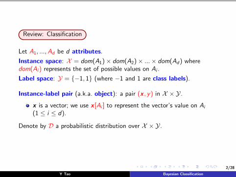
Review: Classification
Let A1, ...,Ad be d attributes.
Instance space: X = dom(A1)× dom(A2)× ...× dom(Ad) wheredom(Ai ) represents the set of possible values on Ai .
Label space: Y = {−1, 1} (where −1 and 1 are class labels).
Instance-label pair (a.k.a. object): a pair (x , y) in X × Y.
x is a vector; we use x [Ai ] to represent the vector’s value on Ai
(1 ≤ i ≤ d).
Denote by D a probabilistic distribution over X × Y.
Y Tao Bayesian Classification
3/28
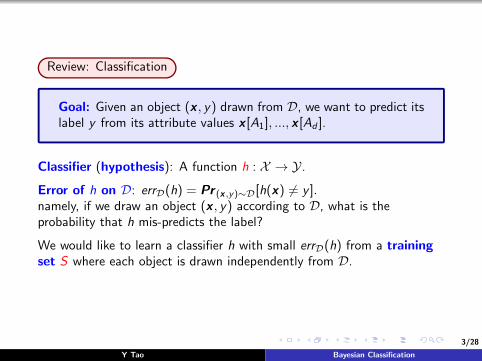
Review: Classification
Goal: Given an object (x , y) drawn from D, we want to predict itslabel y from its attribute values x [A1], ..., x [Ad ].
Classifier (hypothesis): A function h : X → Y.
Error of h on D: errD(h) = Pr (x,y)∼D[h(x) 6= y ].namely, if we draw an object (x , y) according to D, what is theprobability that h mis-predicts the label?
We would like to learn a classifier h with small errD(h) from a trainingset S where each object is drawn independently from D.
Y Tao Bayesian Classification
4/28
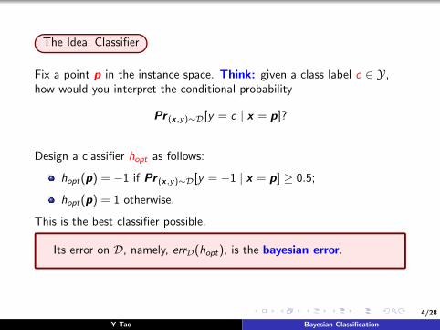
The Ideal Classifier
Fix a point p in the instance space. Think: given a class label c ∈ Y,how would you interpret the conditional probability
Pr (x,y)∼D[y = c | x = p]?
Design a classifier hopt as follows:
hopt(p) = −1 if Pr (x,y)∼D[y = −1 | x = p] ≥ 0.5;
hopt(p) = 1 otherwise.
This is the best classifier possible.
Its error on D, namely, errD(hopt), is the bayesian error.
Y Tao Bayesian Classification
5/28
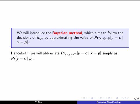
We will introduce the Bayesian method, which aims to follow thedecisions of hopt by approximating the value of Pr (x,y)∼D[y = c |x = p].
Henceforth, we will abbreviate Pr (x,y)∼D[y = c | x = p] simply as
Pr [y = c | p].
Y Tao Bayesian Classification
6/28
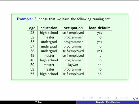
Example: Suppose that we have the following traning set:
age education occupation loan default28 high school self-employed yes32 master programmer no33 undergrad programmer yes37 undergrad programmer no38 undergrad self-employed yes45 master self-employed no48 high school programmer no50 master laywer no52 master programmer no55 high school self-employed no
Y Tao Bayesian Classification
7/28
Bayesian classification works most effectively when each attributehas a small domain, namely, the attribute has only a small numberof possible values. When an attribute has a large domain, we mayreduce its domain size through discretization.
For example, we may discretize the “age” attribute into a smaller
domain: {20+, 30+, 40+, 50+}, where “20+” corresponds to the interval
[20, 29], “30+” to [30, 39], and so on. See the next slide for the training
set after the conversion.
Y Tao Bayesian Classification
8/28
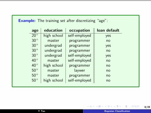
Example: The training set after discretizing “age”:
age education occupation loan default20+ high school self-employed yes30+ master programmer no30+ undergrad programmer yes30+ undergrad programmer no30+ undergrad self-employed yes40+ master self-employed no40+ high school programmer no50+ master laywer no50+ master programmer no50+ high school self-employed no
Y Tao Bayesian Classification
9/28
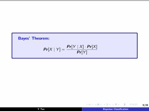
Bayes’ Theorem:
Pr [X | Y ] =Pr [Y | X ] · Pr [X ]
Pr [Y ]
Y Tao Bayesian Classification

10/28
Given an instance x , (as in hopt) we predict its label as −1 if and only if
Pr [y = −1 | x ] ≥ Pr [y = 1 | x ].
Applying Bayes’ theorem, we get:
Pr [y = 1 | x ] =Pr [x | y = 1] · Pr [y = 1]
Pr [x ].
Similarly:
Pr [y = −1 | x ] =Pr [x | y = −1] · Pr [y = −1]
Pr [x ].
It suffices to decide which of the following is larger:
Pr [x | y = 1] · Pr [y = 1], or
Pr [x | y = −1] · Pr [y = −1].
Y Tao Bayesian Classification
11/28
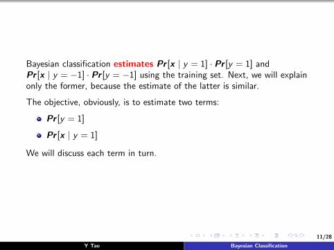
Bayesian classification estimates Pr [x | y = 1] · Pr [y = 1] andPr [x | y = −1] · Pr [y = −1] using the training set. Next, we will explainonly the former, because the estimate of the latter is similar.
The objective, obviously, is to estimate two terms:
Pr [y = 1]
Pr [x | y = 1]
We will discuss each term in turn.
Y Tao Bayesian Classification
12/28
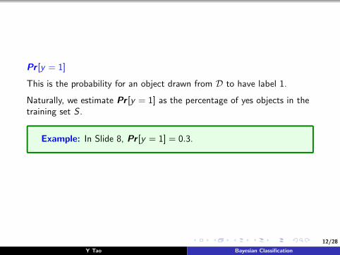
Pr [y = 1]
This is the probability for an object drawn from D to have label 1.
Naturally, we estimate Pr [y = 1] as the percentage of yes objects in thetraining set S .
Example: In Slide 8, Pr [y = 1] = 0.3.
Y Tao Bayesian Classification

13/28
Pr [x | y = 1]
This is the probability for a “yes”-object drawn from D to carry exactlythe attribute values x [A1], ..., x [Ad ].
We could estimate Pr [x | y = 1] as the percentage of objects havingattribute values x [A1], ..., x [Ad ] among all the yes objects in S . But thisis a bad idea because S may have very few (even none) such objects,rendering the estimate unreliable (losing statistical significance).
This situation forces us to introduce assumptions which — if satisfied —
would allow us to obtain a more reliable estimate of Pr [x | y = 1].
Y Tao Bayesian Classification
14/28
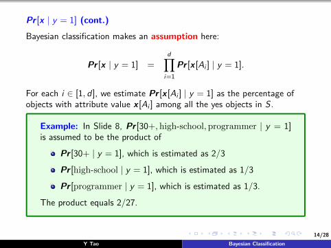
Pr [x | y = 1] (cont.)
Bayesian classification makes an assumption here:
Pr [x | y = 1] =d∏
i=1
Pr [x [Ai ] | y = 1].
For each i ∈ [1, d ], we estimate Pr [x [Ai ] | y = 1] as the percentage ofobjects with attribute value x [Ai ] among all the yes objects in S .
Example: In Slide 8, Pr [30+,high-school,programmer | y = 1]is assumed to be the product of
Pr [30+ | y = 1], which is estimated as 2/3
Pr [high-school | y = 1], which is estimated as 1/3
Pr [programmer | y = 1], which is estimated as 1/3.
The product equals 2/27.
Y Tao Bayesian Classification

15/28
Pr [x | y = 1] (cont.)
The estimate of Pr [x [Ai ] | y = 1] would be 0 if S does not have anyyes-object with attribute value x [Ai ]. But that would force our estimateof Pr [x | y = 1] to be 0. Instead, we replace the 0 estimate with a verysmall value, for example, 0.000001.
Example: In Slide 8, Pr [lawyer | y = 1] is estimated as 0.000001.
Think: At the beginning, we said that Bayesian classification worksbetter on small domains. Why?
Y Tao Bayesian Classification

16/28
The effectiveness of Bayesian classification relies on the accuracy of theassumption:
Pr [x | y = 1] =d∏
i=1
Pr [x [Ai ] | y = 1].
This assumption is called the conditional independence assumption.When this assumption is seriously violated, the accuracy of the methoddrops significantly.
Y Tao Bayesian Classification
17/28
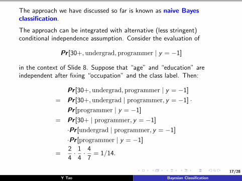
The approach we have discussed so far is known as naive Bayesclassification.
The approach can be integrated with alternative (less stringent)conditional independence assumption. Consider the evaluation of
Pr [30+,undergrad,programmer | y = −1]
in the context of Slide 8. Suppose that “age” and “education” areindependent after fixing “occupation” and the class label. Then:
Pr [30+,undergrad,programmer | y = −1]
= Pr [30+,undergrad | programmer, y = −1] ·Pr [programmer | y = −1]
= Pr [30+ | programmer, y = −1]
·Pr [undergrad | programmer, y = −1]
·Pr [programmer | y = −1]
=2
4· 1
4· 4
7= 1/14.
Y Tao Bayesian Classification
18/28
Next, we will provide an alternative way to describe the Bayesmethod (using naive Bayes as an example). Our description willclarify what is actually the set H of classifiers to be learned from.This allows you to apply the generalization theorem (discussed inthe previous lecture) to bound the generalization error of the clas-sifier obtained.
Y Tao Bayesian Classification
19/28
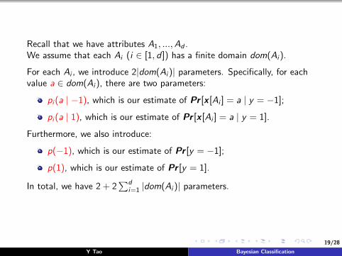
Recall that we have attributes A1, ...,Ad .We assume that each Ai (i ∈ [1, d ]) has a finite domain dom(Ai ).
For each Ai , we introduce 2|dom(Ai )| parameters. Specifically, for eachvalue a ∈ dom(Ai ), there are two parameters:
pi (a | −1), which is our estimate of Pr [x [Ai ] = a | y = −1];
pi (a | 1), which is our estimate of Pr [x [Ai ] = a | y = 1].
Furthermore, we also introduce:
p(−1), which is our estimate of Pr [y = −1];
p(1), which is our estimate of Pr [y = 1].
In total, we have 2 + 2∑d
i=1 |dom(Ai )| parameters.
Y Tao Bayesian Classification

20/28
Once the values of the 2 + 2∑d
i=1 |dom(Ai )| parameters have been fixed,the conditional independence assumption (of naive Bayes) gives rise tothe following classifier h(x):
h(x) = −1 if
p(−1) ·d∏
i=1
pi (x [Ai ] | −1) ≥ p(1) ·d∏
i=1
pi (x [Ai ] | 1)
h(x) = 1 otherwise.
The set H contains all such classifiers.
Remark: The Bayes method we explained earlier gives an efficientway for choosing a reasonably good classifier h ∈ H.
Y Tao Bayesian Classification
21/28
Next, we introduce the Bayesian network which is a popular wayto describe sophisticated conditional independence assumptions.
Let us review some concepts on acyclic directed graphs (DAG):
A DAG G is a directed graph with no cycles.
A node in G with 0 in-degree is a root. Note that G may havemultiple roots.
If a node u has an edge to another node v , then u is a parent of v .Note that a node can have multiple parents.
We will use parents(v) to represent the set of parents of a node v .
Y Tao Bayesian Classification
22/28
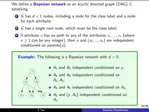
We define a Bayesian network as an acyclic directed graph (DAG) Gsatisfying:
1 G has d + 1 nodes, including a node for the class label and a nodefor each attribute;
2 G has a single root node, which must be the class label;
3 if attribute u has no path to any of the attributes v1, ..., vx (wherex ≥ 1 can be any integer), then u and (v1, ..., vx) are independentconditioned on parents(u).
Example: The following is a Bayesian network with d = 5.
A1
y
A2
A3 A4 A5
A1 and A2 independent conditioned on y ;
A4 and A5 independent conditioned onA1,A2;
A3 and A5 independent conditioned on A1;
A3 and (y ,A5) independent conditioned onA1.
Y Tao Bayesian Classification

23/28
Theorem 1: Given the conditional independence assumptions de-scribed by a Bayesian network G , we have
Pr [A1, ...,Ad | y ] =d∏
i=1
Pr [Ai | parents(Ai )].
Before proving the theorem, let us first see an example.
Example: Given the Bayesian network on the previous slide, wehave:
Pr [A1,A2, ...,A5 | y ] =
Pr [A1 | y ] · Pr [A2 | y ] · Pr [A3 | A1] · Pr [A4 | A1,A2] · Pr [A5 | A1,A2].
Y Tao Bayesian Classification
24/28
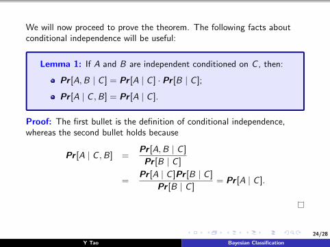
We will now proceed to prove the theorem. The following facts aboutconditional independence will be useful:
Lemma 1: If A and B are independent conditioned on C , then:
Pr [A,B | C ] = Pr [A | C ] · Pr [B | C ];
Pr [A | C ,B] = Pr [A | C ].
Proof: The first bullet is the definition of conditional independence,whereas the second bullet holds because
Pr [A | C ,B] =Pr [A,B | C ]
Pr [B | C ]
=Pr [A | C ]Pr [B | C ]
Pr [B | C ]= Pr [A | C ].
Y Tao Bayesian Classification
25/28
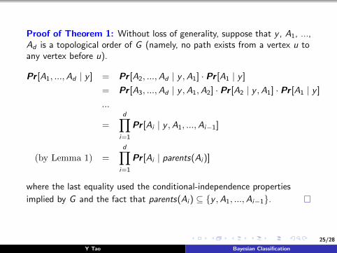
Proof of Theorem 1: Without loss of generality, suppose that y , A1, ...,Ad is a topological order of G (namely, no path exists from a vertex u toany vertex before u).
Pr [A1, ...,Ad | y ] = Pr [A2, ...,Ad | y ,A1] · Pr [A1 | y ]
= Pr [A3, ...,Ad | y ,A1,A2] · Pr [A2 | y ,A1] · Pr [A1 | y ]
...
=d∏
i=1
Pr [Ai | y ,A1, ...,Ai−1]
(by Lemma 1) =d∏
i=1
Pr [Ai | parents(Ai )]
where the last equality used the conditional-independence properties
implied by G and the fact that parents(Ai ) ⊆ {y ,A1, ...,Ai−1}.
Y Tao Bayesian Classification

26/28
Example: Consider the training set on Slide 8. If we are given theBayesian network
occ
y
age edu
then Pr [30+,undergrad,programmer | y = −1] is calculated asshown on Slide 17.
Y Tao Bayesian Classification

27/28
Example (cont.): If the Bayesian network is
occ
y
age edu
then Pr [30+,undergrad,programmer | y = −1]
= Pr [30+,undergrad | programmer, y = −1] ·Pr [programmer | y = −1]
= Pr [30+ | programmer] · Pr [undergrad | programmer]
·Pr [programmer | y = −1]
=3
5· 2
5· 4
7= 24/175.
Y Tao Bayesian Classification
28/28
Think: What is the set H of classifiers to be learned from if weare given the Bayesian network on the previous slide?
Y Tao Bayesian Classification