Bayesian Active Learning for Classification and

Preference Learning

Neil Houlsby, Ferenc Huszar, Zoubin Ghahramani, Mate LengyelComputational and Biological Learning Laboratory

University of Cambridge

December 30, 2011

Abstract

Information theoretic active learning has been widely studied for prob-abilistic models. For simple regression an optimal myopic policy is easilytractable. However, for other tasks and with more complex models, suchas classification with nonparametric models, the optimal solution is harderto compute. Current approaches make approximations to achieve tractabil-ity. We propose an approach that expresses information gain in termsof predictive entropies, and apply this method to the Gaussian ProcessClassifier (GPC). Our approach makes minimal approximations to the fullinformation theoretic objective. Our experimental performance comparesfavourably to many popular active learning algorithms, and has equal orlower computational complexity. We compare well to decision theoreticapproaches also, which are privy to more information and require muchmore computational time. Secondly, by developing further a reformulationof binary preference learning to a classification problem, we extend ouralgorithm to Gaussian Process preference learning.

1 Introduction

In most machine learning systems, the learner passively collects data with whichit makes inferences about its environment. In active learning, however, thelearner seeks the most useful measurements to be trained upon. The goal ofactive learning is to produce the best model with the least possible data; thisis closely related to the statistical field of optimal experimental design. Withthe advent of the internet and expansion of storage facilities, vast quantitiesof unlabelled data have become available, but it can be costly to obtain labels.Finding the most useful data in this vast space calls for efficient active learningalgorithms.

Two approaches to active learning are to use decision and information the-ory [Kapoor et al., 2007, Lindley, 1956]. The former minimizes the expected

1

arX

iv:1

112.

5745

v1 [

stat

.ML

] 2

4 D

ec 2

011

losses encountered after making decisions based on the data collected i.e. min-imize the Bayes posterior risk [Roy and McCallum, 2001]. Maximising perfor-mance under test is the ultimate objective of most learners, however, evaluat-ing this objective can be very hard. For example, the methods proposed in[Kapoor et al., 2007, Zhu et al., 2003] for classification are in general expensiveto compute. Furthermore, one may not know the loss function or test distributionin advance, or may want the model to perform well on a variety of loss functions.In extreme scenarios, such as exploratory data analysis, or visualisation, lossesmay be very hard to quantify.

This motivates information theoretic approaches to active learning, which areagnostic to the decision task at hand and particular test data, this is known aninductive approach. They seek to reduce the number of feasible models as quicklyas possible, using either heuristics (e.g. margin sampling [Tong and Koller, 2001])or by formalising uncertainty using well studied quantities, such as Shannonsentropy and the KL-divergence [Cover et al., 1991]. Although the latter approachwas proposed several decades ago [Lindley, 1956, Bernardo, 1979], it is not alwaysstraightforward to apply the criteria to complicated models such as nonparametricprocesses with infinite parameter spaces. As a result many algorithms existwhich compute approximate posterior entropies, perform sampling, or work withrelated quantities in non-probabilistic models.

We return to this problem, presenting the full information criterion anddemonstrate how to apply it to Gaussian Processes Classification (GPC), yieldinga novel active learning algorithm that makes minimal approximations. GPC is apowerful, non-parametric kernel-based model, and poses an interesting problemfor information-theoretic active learning because the parameter space is infinitedimensional and the posterior distribution is analytically intractable. We presentthe information theoretic approach to active learning in Section 2. In Section3 we apply it to GPC, and show how to extended our method to preferencelearning. In Section 4 we review other approaches and how they compare to ouralgorithm. We take particular care to contrast our approach to the InformativeVector Machine, that addresses data point selection for GPs directly. We presentresults on a wide variety of datasets in Section 5 and conclude in Section 6.

2 Bayesian Information Theoretic Active Learn-ing

We consider a fully discriminative model where the goal of active learning isto discover the dependence of some variable y ∈ Y on an input variable x ∈ X .The key idea in active learning is that the learner chooses the input queriesxi ∈ X and observes the system’s response yi, rather than passively receiving(xiyi) pairs.

Within a Bayesian framework we assume existence of some latent param-eters, θ, that control the dependence between inputs and outputs, p(y|x,θ).Having observed data D = {(xi, yi)}ni=1, a posterior distribution over the pa-

2

rameters is inferred, p(θ|D). The central goal of information theoretic ac-tive learning is to reduce the number possible hypotheses maximally fast, i.e.to minimize the uncertainty about the parameters using Shannon’s entropy[Cover et al., 1991]. Data points D′ are selected that satisfy arg minD′ H[θ|D′] =−∫p(θ|D′) log p(θ|D′)dθ. Solving this problem in general is NP-hard; however,

as is common in sequential decision making tasks a myopic (greedy) approxi-mation is made [Heckerman et al., 1995]. It has been shown that the myopicpolicy can perform near-optimally [Golovin and Krause, 2010, Dasgupta, 2005].Therefore, the objective is to seek the data point x that maximises the decreasein expected posterior entropy:

arg maxx

H[θ|D]− Ey∼p(y|xD) [H[θ|y,x,D]] (1)

Note that expectation over the unseen output y is required. Many workse.g. [MacKay, 1992, Krishnapuram et al., , Lawrence et al., 2003] propose usingthis objective directly. However, parameter posteriors are often high dimen-sional and computing their entropies is usually intractable. Furthermore, fornonparametric processes the parameter space is infinite dimensional so Eqn. (1)becomes poorly defined. To avoid gridding parameter space (exponentially hardwith dimensionality), or sampling (from which it is notoriously hard to estimateentropies without introducing bias [Panzeri and Petersen, 2007]), these papersmake Gaussian or low dimensional approximations and calculate the entropy ofthe approximate posterior. A second computational difficulty arises; if Nx datapoints are under consideration, and Ny responses may be seen, then O(NxNy),potentially expensive, posterior updates are required to calculate Eqn. (1).

An important insight arises if we note that the objective in Eqn. (1) isequivalent to the conditional mutual information between the unknown outputand the parameters, I[θ, y|x,D]. Using this insight it is simple to show that theobjective can be rearranged to compute entropies in y space:

arg maxx

H[y|x,D]− Eθ∼p(θ|D) [H[y|x,θ]] (2)

Eqn. (2) overcomes the challenges we described for Eqn. (1). Entropies are nowcalculated in, usually low dimensional, output space. For binary classification,these are just entropies of Bernoulli variables. Also θ is now conditioned onlyon D, so only O(1) posterior updates are required. Eqn. (2) also provides uswith an interesting intuition about the objective; we seek the x for which themodel is marginally most uncertain about y (high H[y|x,D]), but for whichindividual settings of the parameters are confident (low Eθ∼p(θ|D) [H[y|x,θ]]).This can be interpreted as seeking the x for which the parameters under theposterior disagree about the outcome the most, so we refer to this objective asBayesian Active Learning by Disagreement (BALD). We present a method toapply Eqn. (2) directly to GPC and preference learning. We no longer need tobuild our entropy calculation around the type of posterior approximation (as

3

in [MacKay, 1992, Krishnapuram et al., , Lawrence et al., 2003]) but are free tochoose from many of the available algorithms. Minimal additional approximationsare introduced, and so, to our knowledge our algorithm represents the mostexact and fastest way to perform full information-theoretic active learning innon-parametric discriminative models.

3 Gaussian Processes for Classification and Pref-erence Learning

In this section we derive the BALD algorithm for Gaussian Process classification(GPC). GPs are a powerful and popular non-parametric tool for regressionand classification. GPC appears to be an especially challenging problem forinformation-theoretic active learning because the parameter space is infinite,however, by using (2) we are able to calculate fully the relevant informationquantities without having to work out entropies of infinite dimensional objects.The probabilistic model underlying GPC is as follows:

f ∼ GP(µ(·), k(·, ·))y|x, f ∼ Bernoulli(Φ(f(x)))

The latent parameter, now called f is a function X → R, and is assigned aGaussian process prior with mean µ(·) and covariance function or kernel k(·, ·).We consider the probit case where given the value of f , y takes a Bernoullidistribution with probability Φ(f(x)), and Φ is the Gaussian CDF. For furtherdetails on GPs see [Rasmussen and Williams, 2005].

Inference in the GPC model is intractable; given some observations D, theposterior over f becomes non-Gaussian and complicated. The most commonlyused approximate inference methods – EP, Laplace approximation, AssumedDensity Filtering and sparse methods – all approximate the posterior by aGaussian [Rasmussen and Williams, 2005]. Throughout this section we willassume that we are provided with such a Gaussian approximation from oneof these methods, though the active learning algorithm does not care whichone. In our derivation we will use

1≈ to indicate where such an approximation is

exploited.The informativeness of a query x is computed using Eqn. (2). The entropy

of the binary output variable y given a fixed f can be expressed in terms of thebinary entropy function h:

H[y|x, f ] = h (Φ(f(x))

h(p) = −p log p− (1− p) log(1− p)

Expectations over the posterior need to be computed. Using a Gaussian approxi-mation to the posterior, for each x, fx = f(x) will follow a Gaussian distributionwith mean µx,D and variance σ2

x,D. To compute Eqn. (2) we have to compute

4

two entropy quantities. The first term in Eqn. (2), H[y|x,D] can be handledanalytically for the probit case:

H[y|x,D]1≈ h

(∫Φ(fx)N (fx|µx,D, σ2

x,D)dfx

)

= h

Φ

µx,D√σ2x,D + 1

(3)

The second term, Ef∼p(f |D) [H[y|x, f ]] can be computed approximately as follows:

Ef∼p(f |D) [H[y|x, f ]]

1≈∫

h(Φ(fx))N (fx|µx,D, σ2x,D)dfx (4)

2≈∫

exp

(− f2xπ ln 2

)N (fx|µx,D, σ2

x,D)dfx

=C√

σ2x,D + C2

exp

− µ2x,D

2(σ2x,D + C2

)

where C =√

π ln 22 . The first approximation,

1≈, reflects the Gaussian ap-

proximation to the posterior. The integral in the left hand side of Eqn. (4) isintractable. By performing a Taylor expansion on ln h(Φ(fx)) (see supplementarymaterial) we can see that it can be approximated up to O(f4x) by a squaredexponential curve, exp(−f2x/π ln 2). We will refer to this approximation as

2≈.

Now we can apply the standard convolution formula for Gaussians to finally geta closed form expression for both terms of Eqn. (2).

Fig. 1 depicts the striking accuracy of this simple approximation. The max-imum possible error that will be incurred when using this approximation is ifN (fx|µx,D, σ2

x,D) is centred at µx,D = ±2.05 with σ2x,D tending to zero (see

Fig. 1, absolute error ), yielding only a 0.27% error in the integral in Eqn. (4).The authors are unaware of previous use of this simple and useful approximationin this context. In Section 5 we investigate experimentally the information lostfrom approximations

1≈ and

2≈ as compared to the golden standard of extensive

Monte Carlo simulation.To summarise, the BALD algorithm for Gaussian process classification con-

sists of two steps. First it applies any standard approximate inference algorithmfor GPCs (such as EP) to obtain the posterior predictive mean µx,D and σx,D foreach point of interest x. Then, it selects a query x that maximises the followingobjective function:

h

Φ

µx,D√σ2x,D + 1

− C exp

(− µ2

x,D

2(σ2x,D+C2)

)√σ2x,D + C2

(5)

5

−5 0 50

1h(Φ(·))

exp( −t2π log(2)

)

0

5 · 10−3difference

Figure 1: Analytic approximation (1≈) to the binary entropy of the error function

( ) by a squared exponential ( ). The absolute error ( ) remains under3 · 10−3.

For most practically relevant kernels, the objective (5) is a smooth anddifferentiable function of x, so gradient-based optimisation procedures can beused to find the maximally informative query.

3.1 Extension: Learning Hyperparameters

In many applications the parameter set θ naturally divides into parameters ofinterest, θ+, and nuisance parameters θ−, i.e. θ = {θ+,θ−}. In such settings,the active learning may want to query points that are maximally informativeabout θ+, while not caring about θ−. By integrating Eqn. (1) over the nuisanceparameters, θ−, BALD’s objective is re-derived as:

H[Ep(θ+,θ−|D)

[y|x,θ+,θ−

]]− Ep(θ+|D)

[H[Ep(θ−|θ+,D)[y|x,θ+,θ−]

]](6)

In the context of GP models, hyperparameters typically control the smooth-ness or spatial length-scale of functions. If we maintain a posterior distributionover these hyperparameters, which we can do e. g. via Hamiltonian Monte Carlo,we can choose either to treat them as nuisance parameters θ− and use Eq. 6, or toinclude them in θ+ and perform active learning over them as well. In certain cases,such as automatic relevance determination [Rasmussen and Williams, 2005], itmay even make sense to treat hyperparameters as variables of primary interest,and the function f itself as nuisance parameter θ−.

3.2 Preference Learning

Our active learning framework for GPC can be extended to the important problemof preference learning [Furnkranz and Hullermeier, 2003, Chu and Ghahramani, 2005].In preference learning the dataset consists for pairs of items (ui,vi) ∈ X 2 withbinary labels, yi ∈ {0, 1}. yi = 1 means instance ui is preferred to vi, denotedui � vi. The task is to predict the preference relation between any (u,v).We can view this as a special case of building a classifier on pairs of inputs

6

h : X 2 7→ {0, 1}. [Chu and Ghahramani, 2005] propose a Bayesian approach,using a latent preference function f , over which a GP prior is defined. Themodel predicts preference, ui � vi whenever f(ui) + εui

> f(vi) + εvi , whereεui, εvi denote additive Gaussian noise. Under this model, the likelihood of f

becomes:

P[y = 1|(ui,vi), f ] = P[ui � vi|f ]

= Φ

(f(ui)− f(vi)√

2σnoise

)(7)

By rescaling the latent function f , it can be assumed w.l.o.g. that√

2σnoise =1. The likelihood only depends on the difference between f(u) and f(v). Wetherefore define g(u,v) = f(u) − f(v), and do inference entirely in termsof g, for which the likelihood becomes the same as for probit classification:y|u,v, f ∼ Bernoulli(Φ(g(u,v))). We observe that a GP prior is induced on gbecause it is formed by performing a linear operation on f , for which we have aGP prior already f ∼ GP(0, k). We can derive the induced covariance functionof g as (derivation in the Supplementary material) as: kpref((ui,vi), (uj ,vj)) =k(ui,uj) + k(vi,vj)− k(ui,vj)− k(vi,uj).

Note that this kernel kpref respects the anti-symmetry properties desired fora preference learning scenario, i.e. the value g(u, v) is perfectly anti-correlatedwith g(v, u), ensuring P[u � v] = 1 − P[v � u] holds. Thus, we can concludethat the GP preference learning framework of [Chu and Ghahramani, 2005], isequivalent to GPC with a particular class of kernels, that we may call thepreference judgement kernels. Therefore, our active learning algorithm presentedin Section 3 for GPC can readily be applied to pairwise preference learning also.

4 Related Methodologies

There are a number of closely related algorithms for active classification whichwe now review.

The Informative Vector Machine (IVM): Perhaps the most closely re-lated approach is the IVM [Lawrence et al., 2003]. This popular,and successfulapproach to active learning was designed specifically for GPs; it uses an infor-mation theoretic approach and so appears very similar to BALD. The IVMalgorithm was designed for subsampling a dataset for training a GP, so it is privyto the y values before including a measurement; it cannot therefore work explic-itly in output space i.e. with Eqn. (2). The IVM uses Eqn. (1), but parameterentropies are calculated approximately in the marginal subspace correspondingto the observed data points. The entropy decrease after inclusion of a new datapoint can then be calculated efficiently using the GP covariance matrix.

Although the IVM and BALD are motivated by the same objective, they workfundamentally differently when approximate inference is carried out. At any time

7

both methods have an approximate posterior qt(θ|D), this can be updated withthe likelihood of a new data point p(yt+1|f,xt+1), yielding pt+1(θ|D,xt+1, yt+1) =1Z qt(θ|D)p(yt+1|f,xt+1). If the posterior at t+ 1 is approximated directly onegets qt+1(θ|D,xt+1, yt+1). BALD calculates the entropy difference between qtand pt+1, without having to compute qt+1 for each candidate x. In contrast,the IVM calculates the entropy change between qt and qt+1. The IVM’s ap-proach cannot calculate the entropy of the full infinite dimensional posterior,and requires O(NxNy) posterior updates. To do these updates efficiently, ap-proximate inference is performed using Assumed Density Filtering (ADF). UsingADF means that qt+1 is a direct approximation to pt+1, indicating that theIVM makes a further approximation to BALD. Since BALD only requires O(1)posterior updates it can afford to use more accurate, iterative procedures, suchas EP.

Information Theoretic approaches: Maximum Entropy Sampling (MES)[Sebastiani and Wynn, 2000] explicitly works in dataspace (Eqn. (2)). MES wasproposed for regression models with input-independent observation noise. Al-though Eqn. (2) is used, the second term is constant because of input independentnoise and is ignored. One cannot, however, use MES for heteroscedastic re-gression or classification; it fails to differentiate between model uncertainty andobservation uncertainty (about which our model may be confident). Some toydemonstrations show this ‘information based’ active learning criterion performingpathologically in classification by repeatedly querying points close the decisionboundary or in regions of high observation uncertainty e.g. [Huang et al., 2010].This is because MES is inappropriate in this domain; BALD distinguishes be-tween observation and model uncertainty and eliminates these problems as wewill show.

Mutual-information based objective functions are presented in [Ertin et al., ,Fuhrmann, 2003]. They maximise the mutual information between the variablebeing measured and the variable of interest. Fuhrmann [Fuhrmann, 2003] appliesthis to linear Gaussian models and acoustic arrays, Ertin et al. [Ertin et al., ] toa communications channel. Although related, these objectives do not work withthe model parameters and are not applied to classification. [Guestrin et al., 2005,Krause et al., 2006] also use mutual information. They specify interest points inadvance and maximise the expected mutual information between the predictivedistributions at these points and at the observed locations. Although thisis a objective is promising for regression, it is not tractable for models withinput-dependent observation noise, such as classification or preference learning.

Decision theoretic: We briefly mention decision theoretic approaches to ac-tive learning. Two closely related algorithms, [Kapoor et al., 2007, Zhu et al., 2003],seek to minimize the expected cost i.e. loss weighted misclassification probabilityon all seen and future data. These methods observe the locations of the testpoints and their objective functions become monotonic in the predictive entropiesat the test points. [Kapoor et al., 2007] also includes an empirical error term

8

MCMC EP (1≈) Laplace (

1≈)

MC 0 7.51± 2.51 41.57± 4.022≈ 0.16± 0.05 7.43± 2.40 40.45± 3.67

Figure 2: Percentage approximation error (±1 s.d.) for different methods ofapproximate inference (columns) and approximation methods for evaluatingEqn. (4) (rows). The results indicate that

2≈ is a very accurate approximation;

EP causes some loss and Laplace significantly more, which is in line with thecomparison presented in [Kuss and Rasmussen, 2005]. For our experiments weuse EP.

that can yield pathological behaviour (we investigate this experimentally). Theseapproaches are computationally expensive, requiring O(NxNy) posterior updates.Also, they must know the locations of the test data (and thus are transductiveapproaches); designing an inductive, decision-theoretic algorithm is an open,hard problem as it would require expensive integration over possible test datadistributions.

Non-probabilistic Some non-probabilistic methods have close analogues toinformation theoretic active learning. Perhaps the most ubiquitous is activelearning for SVMs [Tong and Koller, 2001, Seung et al., 1992], where the volumeof Version Space (VS) is used as a proxy for the posterior entropy. If a uniform(improper) prior is used with a deterministic classification likelihood, the logvolume of VS and Bayesian posterior entropy are in fact equivalent. Just asBayesian posteriors become intractable after observing many data points, VS canbecome complicated. [Tong and Koller, 2001] proposes methods for approximat-ing VS with a simple shapes, such as hyperspheres (their simplest approximationreduces to margin sampling). This closely resembles approximating a Bayesianposterior using a Gaussian distribution via the Laplace or EP approximations.[Seung et al., 1992] sidesteps the problem by working with predictions. The al-gorithm, Query by Committee (QBC), samples parameters from VS (committeemembers), they vote on the outcome of each possible x. The x with the mostbalanced vote is selected; this is termed the ‘principle of maximal disagreement’.If BALD is used with a sampled posterior, query by committee is implementedbut with a probabilistic measure of disagreement. QBC’s deterministic votecriterion discards confidence in the predictions and so can exhibit the samepathologies as MES.

5 Experiments

Quantifying Approximation Losses: To obtain (5) we made two approx-imations: we perform approximate inference (

1≈), and we approximated the

binary entropy of the Gaussian CDF by a squared exponential (2≈). Both of

these can be substituted with Monte Carlo sampling, enabling us to compute

9

Dim. 1

Dim

.2

(a) block in the middle

Dim. 1

Dim

.2

(b) block in the corner

Dim. 1

Dim

.2

(c) checkerboard

0 20 40

0.5

0.9

No. queried points

Acc

ura

cy

0 25 500.5

1

No. queried points

Acc

ura

cy

0 25 500.5

1

No. queried points

Acc

ura

cy

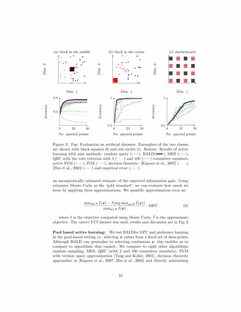
Figure 3: Top: Evaluation on artificial datasets. Exemplars of the two classesare shown with black squares ( ) and red circles ( ). Bottom: Results of activelearning with nine methods: random query ( ), BALD( ), MES ( ),QBC with the vote criterion with 2 ( ) and 100 ( ) committee members,active SVM ( ), IVM ( ), decision theoretic: [Kapoor et al., 2007] ( ),[Zhu et al., 2003] ( ) and empirical error ( ).

an asymptotically unbiased estimate of the expected information gain. Usingextensive Monte Carlo as the ‘gold standard’, we can evaluate how much weloose by applying these approximations. We quantify approximation error as:

maxx∈P I(x)− I(arg maxx∈P I(x))

maxx∈P I(x)· 100% (8)

where I is the objective computed using Monte Carlo, I is the approximateobjective. The cancer UCI dataset was used, results and discussion are in Fig. 2.

Pool based active learning: We test BALDfor GPC and preference learningin the pool-based setting i.e. selecting x values from a fixed set of data-points.Although BALD can generalise to selecting continuous x, this enables us tocompare to algorithms that cannot. We compare to eight other algorithms:random sampling, MES, QBC (with 2 and 100 committee members), SVMwith version space approximation [Tong and Koller, 2001], decision theoreticapproaches in [Kapoor et al., 2007, Zhu et al., 2003] and directly minimizing

10

0 20 400.5

1

No. queried points

Acc

ura

cy

(a) crabs

0 50 100

0.5

1

No. queried points

Acc

ura

cy

(b) vehicle

0 30 600.6

1

No. queried points

Acc

ura

cy

(c) wine

0 25 500.6

1

No. queried points

Acc

ura

cy

(d) wdbc

0 50 100

0.5

1

No. queried points

Acc

ura

cy(e) isolet

0 500.5

0.75

No. queried points

Acc

ura

cy

(f) austra

0 30 600.7

1

No. queried points

Acc

ura

cy

(g) letter D vs. P

0 50 1000.7

1

No. queried points

Acc

ura

cy

(h) letter E vs. F

0 500.5

0.75

No. queried points

Acc

ura

cy

(j) cancer

0 100 200

0.5

0.6

No. queried points

Acc

ura

cy

(j) pref: kinematics

0 30 600.6

1

No. queried points

Acc

ura

cy

(k) pref: cart

0 150 3000.55

0.7

No. queried points

Acc

ura

cy

(l) pref: cpu

Figure 4: Test set classification accuracy on classification and preference learningdatasets. Methods used are BALD( ), random query ( ), MES ( ),QBC with 2 (QBC2, ) and 100 (QBC100, ) committee members, activeSVM ( ), IVM ( ), decision theoretic [Kapoor et al., 2007] ( ), deci-sion theoretic [Zhu et al., 2003] ( ) and empicial error ( ). The decisiontheoretic methods took a long time to run, so were not completed for all datasets.Plots (a-i) are GPC datasets, (j-l) are preference learning.. 11

0

50

100

BALD

Ran

d

IVM

ME

S

QB

C2

QB

C100

SV

M

Kap

oor

Zhuet

al.

Em

pir

ical

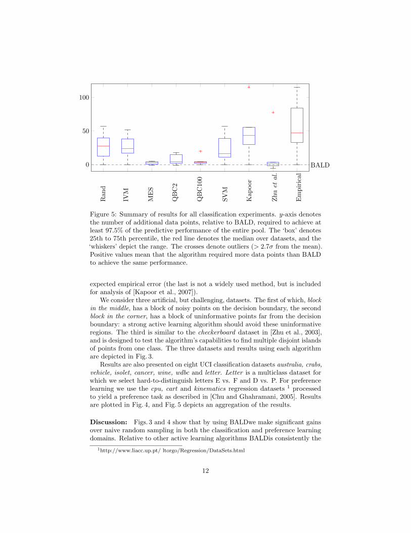
Figure 5: Summary of results for all classification experiments. y-axis denotesthe number of additional data points, relative to BALD, required to achieve atleast 97.5% of the predictive performance of the entire pool. The ‘box’ denotes25th to 75th percentile, the red line denotes the median over datasets, and the‘whiskers’ depict the range. The crosses denote outliers (> 2.7σ from the mean).Positive values mean that the algorithm required more data points than BALDto achieve the same performance.

expected empirical error (the last is not a widely used method, but is includedfor analysis of [Kapoor et al., 2007]).

We consider three artificial, but challenging, datasets. The first of which, blockin the middle, has a block of noisy points on the decision boundary, the secondblock in the corner, has a block of uninformative points far from the decisionboundary: a strong active learning algorithm should avoid these uninformativeregions. The third is similar to the checkerboard dataset in [Zhu et al., 2003],and is designed to test the algorithm’s capabilities to find multiple disjoint islandsof points from one class. The three datasets and results using each algorithmare depicted in Fig. 3.

Results are also presented on eight UCI classification datasets australia, crabs,vehicle, isolet, cancer, wine, wdbc and letter. Letter is a multiclass dataset forwhich we select hard-to-distinguish letters E vs. F and D vs. P. For preferencelearning we use the cpu, cart and kinematics regression datasets 1 processedto yield a preference task as described in [Chu and Ghahramani, 2005]. Resultsare plotted in Fig. 4, and Fig. 5 depicts an aggregation of the results.

Discussion: Figs. 3 and 4 show that by using BALDwe make significant gainsover naive random sampling in both the classification and preference learningdomains. Relative to other active learning algorithms BALDis consistently the

1http://www.liacc.up.pt/ ltorgo/Regression/DataSets.html

12

best, or amongst the best performing algorithms on all datasets. On any individ-ual dataset BALD’s performance is often matched because we compare to manymethods, and the more approximate algorithms can have good performanceunder different conditions. Fig. 5 reveals that BALD has the best overall perfor-mance; on average, all other methods require more data points to achieve thesame classification accuracy. Zhu et al.’s decision theoretic approach is closest,the median increase in the number of data points required is 1.4 and zero (i.e.equivalent to BALD) is within the inter-quartile range. This algorithm, however,requires much more computational time and has access to the full set of testinputs, which BALD does not have. MES and QBC appear close in performanceto BALD, but the zero line falls outside both of their inter-quartile ranges.

As expected, MES performs poorly on the noisy dataset (Fig. 3(a)) becauseit discards knowledge of observation noise. When there is zero observation noiseit is equivalent to BALD e.g. Fig. 3(c). On many of the real-world datasets MESperforms as well as BALD e.g. Fig. 4(b, e), indicating that these datasets aremostly noise-free.

The IVM performs well on Fig. 3(c), but pathologically on 3(a); this is dueto the fact that it biases selection towards points from only one class in thenoisy cluster, reducing the posterior entropy rapidly but artificially. However,it also performs significantly worse than BALD on noise-free (indicated byMES’s strong performance) datasets e.g. Fig. 4(b). This implies that the IVM’sposterior approximation or the ADF update are detrimental to the algorithm’sperformance.

QBC often yields only a small decrement in performance, the samplingapproximation is often not too detrimental. However, it performs poorly on thenoisy artificial dataset (Fig. 3(a)) because the vote criterion is not maintaininga notion of inherent uncertainty, like MES. The SVM-based approach exhibitsvariable performance (it does well on Fig. 4(d), but very poorly on 4(f)). Theperformance is greatly effected by the approximation used, for consistency wepresent here one that yielded the most consistent good performance.

Decision theoretic approaches sometimes perform well, on 3(c) they choosethe first 16 points from the centre of each cluster as they are influenced by thesurrounding unlabelled points. BALDdoes not observe the unlabelled points somay not pick points from the centres. Fig. 5 reveals that BALD is performingas well as the method in [Zhu et al., 2003], and outperforms the approach in[Kapoor et al., 2007], despite not having access to the locations of the testpoints and having a significantly lower computational cost. The objective in[Kapoor et al., 2007] can fail, this is because one term in their objective functionis the empirical error. The weight given to this term is determined by the relativesizes of the training and test set (and the associated losses). Directly minimizingempirical error usually performs very pathologically, picking only ‘safe’ points.When the method in [Kapoor et al., 2007] assigns too much weight to this term,it can fail also.

Finally we note that BALD may occasionally perform poorly on the first fewdata points (e.g. Fig. 4(l)). This is may be because the hyperparameters arefixed throughout the experiments to provide a fair comparison to algorithms

13

incapable of incorporating hyperparameter learning. This may mean that givenlittle data the GP model overfits, leading to BALD selecting abnormal querylocations. Maintaining a distribution over hyperparameters can be done usingMCMC, although this significantly increases computational time. Designing ageneral method to do this efficiently is a subject of further work. In practice, asimple heuristic such as picking the first few points randomly, and optimisinghyperparameters will usually suffice.

6 Conclusions

We have demonstrated a method that applies the full information theoretic activelearning criterion to GP classification that makes, as far as the authors are aware,the smallest number of approximations to date, and has as good computationalcomplexity. We extend the GPC model to develop a new preference learningkernel, which enables us to apply our active learning algorithm directly tothis domain also. The method can handle naturally active learning of kernelhyperparameters, which is a hard, mostly unsolved problem, for example inSVM active learning. One notable feature of our approach is that it is agnosticto the approximate inference methods used. This allows us to choose froma whole range of approximate inference methods, including EP, the Laplaceapproximation, ADF or even sparse online learning, and thereby make thetrade off between computational complexity and accuracy. Our experimentalperformance compares favourably to many other active learning methods forclassification, and even decision theoretic methods that have access to the testdata and require much greater computational time.

References

[Bernardo, 1979] Bernardo, J. (1979). Expected information as expected utility.The Annals of Statistics, 7(3):686–690.

[Chu and Ghahramani, 2005] Chu, W. and Ghahramani, Z. (2005). Preferencelearning with Gaussian processes. In ICML, pages 137–144. ACM.

[Cover et al., 1991] Cover, T., Thomas, J., and Wiley, J. (1991). Elements ofinformation theory, volume 6. Wiley Online Library.

[Dasgupta, 2005] Dasgupta, S. (2005). Analysis of a greedy active learningstrategy. In NIPS.

[Ertin et al., ] Ertin, E., Fisher, J., and Potter, L. Maximum mutual informationprinciple for dynamic sensor query problems. In Information Processing inSensor Networks, Lecture Notes in Computer Science.

[Fuhrmann, 2003] Fuhrmann, D. (2003). Active Testing Surveillance Systems,or, Playing Twenty Questions with a Radar. Defense Technical InformationCenter.

14

[Furnkranz and Hullermeier, 2003] Furnkranz, J. and Hullermeier, E. (2003).Pairwise preference learning and ranking. Machine Learning: ECML 2003,pages 145–156.

[Golovin and Krause, 2010] Golovin, D. and Krause, A. (2010). Adaptive sub-modularity: A new approach to active learning and stochastic optimization.In COLT.

[Guestrin et al., 2005] Guestrin, C., Krause, A., and Singh, A. P. (2005). Near-optimal sensor placements in Gaussian processes. In Proceedings of the 22ndinternational conference on Machine learning, ICML ’05, pages 265–272, NewYork, NY, USA. ACM.

[Heckerman et al., 1995] Heckerman, D., Breese, J., and Rommelse, K. (1995).Troubleshooting under uncertainty. Communications of the ACM, 38(3):27–41.

[Huang et al., 2010] Huang, S., Jin, R., and Zhou, Z. (2010). Active learningby querying informative and representative examples. Advances in neuralinformation processing systems, 23:892–900.

[Kapoor et al., 2007] Kapoor, A., Horvitz, E., and Basu, S. (2007). Selective su-pervision: Guiding supervised learning with decision-theoretic active learning.In IJCAI.

[Krause et al., 2006] Krause, A., Guestrin, C., Gupta, A., and Kleinberg, J.(2006). Near-optimal sensor placements: Maximizing information while mini-mizing communication cost. In Proceedings of the 5th international conferenceon Information processing in sensor networks, pages 2–10. ACM.

[Krishnapuram et al., ] Krishnapuram, B., Williams, D., Xue, Y., Hartemink,A., Carin, L., and Figueiredo, M. On semi-supervised classification. NIPS.

[Kuss and Rasmussen, 2005] Kuss, M. and Rasmussen, C. E. (2005). Assesingapproximations for gaussian process classification. In NIPS. MIT Press.

[Lawrence et al., 2003] Lawrence, N., Seeger, M., and Herbrich, R. (2003). Fastsparse Gaussian Process methods: The informative vector machine. Advancesin neural information processing systems, pages 625–632.

[Lindley, 1956] Lindley, D. (1956). On a measure of the information providedby an experiment. The Annals of Mathematical Statistics, 27(4):986–1005.

[MacKay, 1992] MacKay, D. (1992). Information-based objective functions foractive data selection. Neural computation, 4(4):590–604.

[Panzeri and Petersen, 2007] Panzeri, S., S. R. M. M. and Petersen, R. (2007).Correcting for the sampling bias problem in spike train information measures.Journal of neurophysiology, 98(3):1064.

[Rasmussen and Williams, 2005] Rasmussen, C. and Williams, C. (2005). Gaus-sian Processes for Machine Learning. The MIT Press.

15

[Roy and McCallum, 2001] Roy, N. and McCallum, A. (2001). Toward optimalactive learning through sampling estimation of error reduction. In ICML,pages 441–448.

[Sebastiani and Wynn, 2000] Sebastiani, P. and Wynn, H. (2000). Maximumentropy sampling and optimal Bayesian experimental design. Journal of theRoyal Statistical Society: Series B (Statistical Methodology), 62(1):145–157.

[Seung et al., 1992] Seung, H., Opper, M., and Sompolinsky, H. (1992). Queryby committee. In COLT, pages 287–294. ACM.

[Tong and Koller, 2001] Tong, S. and Koller, D. (2001). Support vector machineactive learning with applications to text classification. Journal of MachineLearning Research, 2:45–66.

[Zhu et al., 2003] Zhu, X., Ghahramani, Z., and Lafferty, J. (2003). Combiningactive learning and semi-supervised learning using Gaussian fields and har-monic functions. ICML 2003 workshop on The Continuum from Labeled toUnlabeled Data in Machine Learning and Data Mining.

16

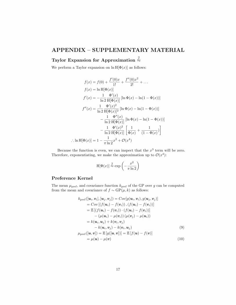
APPENDIX – SUPPLEMENTARY MATERIAL

Taylor Expansion for Approximation2≈

We perform a Taylor expansion on ln H[Φ(x)] as follows:

f(x) = f(0) +f ′(0)x

1!+f ′′(0)x2

2!+ . . .

f(x) = ln H[Φ(x)]

f ′(x) = − 1

ln 2

Φ′(x)

H[Φ(x)][ln Φ(x)− ln(1− Φ(x))]

f ′′(x) =1

ln 2

Φ′(x)2

H[Φ(x)]2[ln Φ(x)− ln(1− Φ(x))]

− 1

ln 2

Φ′′(x)

H[Φ(x)][ln Φ(x)− ln(1− Φ(x))]

− 1

ln 2

Φ′(x)2

H[Φ(x)]

[1

Φ(x)+

1

(1− Φ(x))

]∴ ln H[Φ(x)] = 1− 1

π ln 2x2 +O(x4)

Because the function is even, we can inspect that the x3 term will be zero.Therefore, exponentiating, we make the approximation up to O(x4):

H[Φ(x)]2≈ exp

(− x2

π ln 2

)

Preference Kernel

The mean µpref , and covariance function kpref of the GP over g can be computedfrom the mean and covariance of f ∼ GP(µ, k) as follows:

kpref([ui,vi], [uj ,vj ]) = Cov[g(ui,vi), g(uj ,vj)]

= Cov [(f(ui)− f(vi)) , (f(ui)− f(vi))]

= E [(f(ui)− f(vi)) · (f(ui)− f(vi))]

− (µ(ui)− µ(vi)) (µ(vj)− µ(ui))

= k(ui,uj) + k(vi,vj)

− k(ui,vj)− k(vi,uj) (9)

µpref([u,v]) = E [g([u,v])] = E [f(u)− f(v)]

= µ(u)− µ(v) (10)

17