basics of helio- and asteroseismology

Basics of helio- and asteroseismology

Anna Ogorzałek?, Supervisor: Professor Hiromoto ShibahashiJagiellonian University, University of Tokyo Summer Research Internship Program

October 20, 2011

ABSTRACTThis is a report from my project at University of Tokyo Research Internship Program2011. During my stay at Todai I was learning about basic physics, mathematicaland computational tools that are currently being used in helio- and asteroseismology.This science is the only tool allowing us to learn about stellar interiors. For betterunderstanding of the problem I was developing and using simple model (polytropemodel) to construct solutions of equations, calculate frequencies and physical profilesof the star.

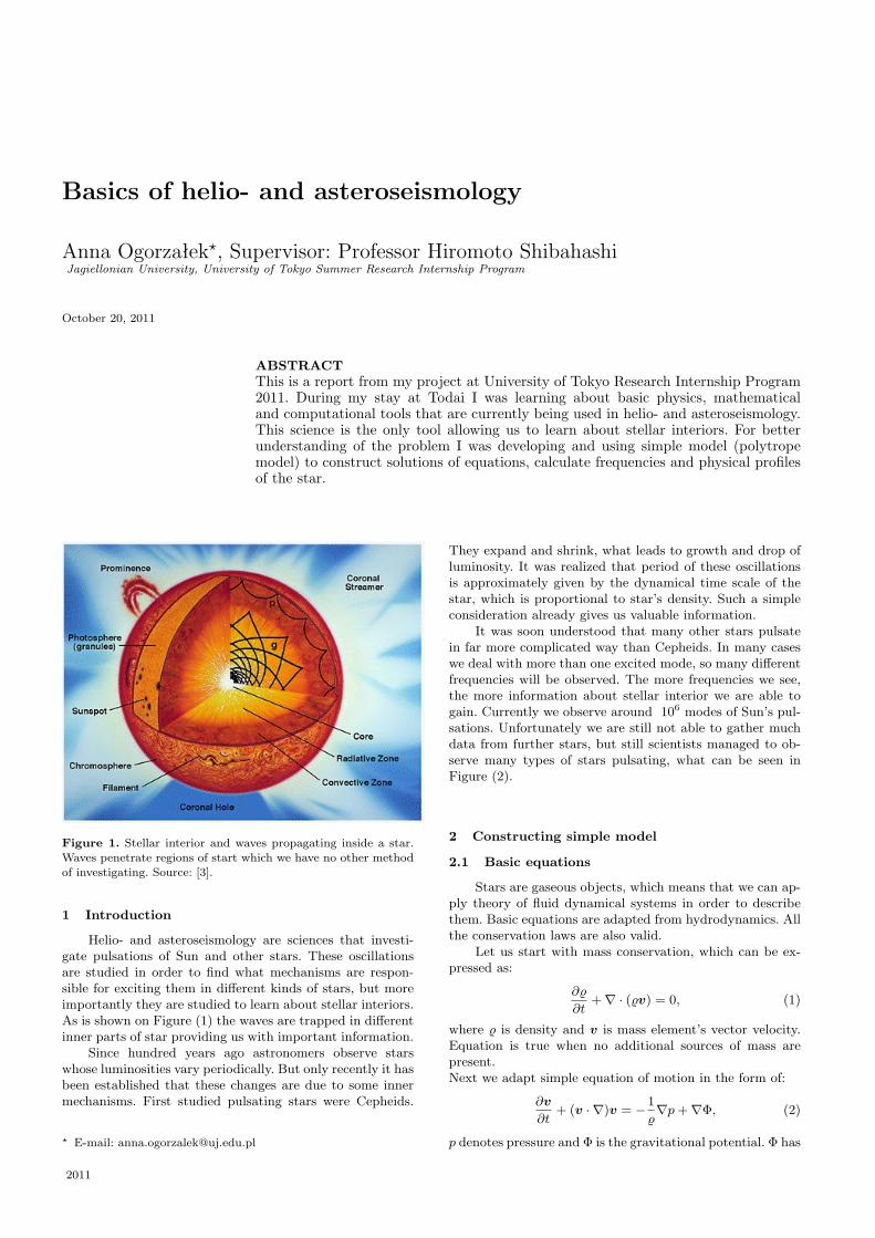
Figure 1. Stellar interior and waves propagating inside a star.Waves penetrate regions of start which we have no other methodof investigating. Source: [3].

1 Introduction

Helio- and asteroseismology are sciences that investi-gate pulsations of Sun and other stars. These oscillationsare studied in order to find what mechanisms are respon-sible for exciting them in different kinds of stars, but moreimportantly they are studied to learn about stellar interiors.As is shown on Figure (1) the waves are trapped in differentinner parts of star providing us with important information.

Since hundred years ago astronomers observe starswhose luminosities vary periodically. But only recently it hasbeen established that these changes are due to some innermechanisms. First studied pulsating stars were Cepheids.

? E-mail: [email protected]

They expand and shrink, what leads to growth and drop ofluminosity. It was realized that period of these oscillationsis approximately given by the dynamical time scale of thestar, which is proportional to star’s density. Such a simpleconsideration already gives us valuable information.

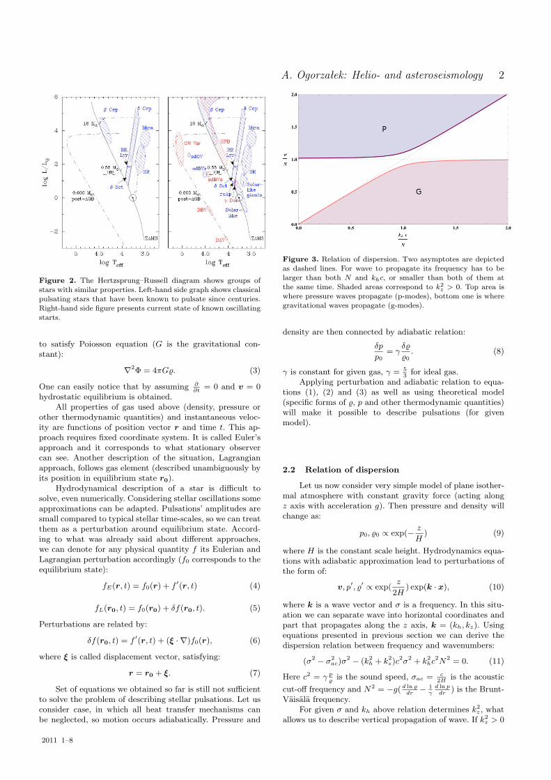
It was soon understood that many other stars pulsatein far more complicated way than Cepheids. In many caseswe deal with more than one excited mode, so many differentfrequencies will be observed. The more frequencies we see,the more information about stellar interior we are able togain. Currently we observe around 106 modes of Sun’s pul-sations. Unfortunately we are still not able to gather muchdata from further stars, but still scientists managed to ob-serve many types of stars pulsating, what can be seen inFigure (2).

2 Constructing simple model

2.1 Basic equations

Stars are gaseous objects, which means that we can ap-ply theory of fluid dynamical systems in order to describethem. Basic equations are adapted from hydrodynamics. Allthe conservation laws are also valid.

Let us start with mass conservation, which can be ex-pressed as:

∂%

∂t+∇ · (%v) = 0, (1)

where % is density and v is mass element’s vector velocity.Equation is true when no additional sources of mass arepresent.Next we adapt simple equation of motion in the form of:

∂v

∂t+ (v · ∇)v = −1

%∇p+∇Φ, (2)

p denotes pressure and Φ is the gravitational potential. Φ has

2011

A. Ogorzałek: Helio- and asteroseismology 2

Figure 2. The Hertzsprung–Russell diagram shows groups ofstars with similar properties. Left-hand side graph shows classicalpulsating stars that have been known to pulsate since centuries.Right-hand side figure presents current state of known oscillatingstarts.

to satisfy Poiosson equation (G is the gravitational con-stant):

∇2Φ = 4πG%. (3)

One can easily notice that by assuming ∂∂t

= 0 and v = 0hydrostatic equilibrium is obtained.

All properties of gas used above (density, pressure orother thermodynamic quantities) and instantaneous veloc-ity are functions of position vector r and time t. This ap-proach requires fixed coordinate system. It is called Euler’sapproach and it corresponds to what stationary observercan see. Another description of the situation, Lagrangianapproach, follows gas element (described unambiguously byits position in equilibrium state r0).

Hydrodynamical description of a star is difficult tosolve, even numerically. Considering stellar oscillations someapproximations can be adapted. Pulsations’ amplitudes aresmall compared to typical stellar time-scales, so we can treatthem as a perturbation around equilibrium state. Accord-ing to what was already said about different approaches,we can denote for any physical quantity f its Eulerian andLagrangian perturbation accordingly (f0 corresponds to theequilibrium state):

fE(r, t) = f0(r) + f ′(r, t) (4)

fL(r0, t) = f0(r0) + δf(r0, t). (5)

Perturbations are related by:

δf(r0, t) = f ′(r, t) + (ξ · ∇)f0(r), (6)

where ξ is called displacement vector, satisfying:

r = r0 + ξ. (7)

Set of equations we obtained so far is still not sufficientto solve the problem of describing stellar pulsations. Let usconsider case, in which all heat transfer mechanisms canbe neglected, so motion occurs adiabatically. Pressure and

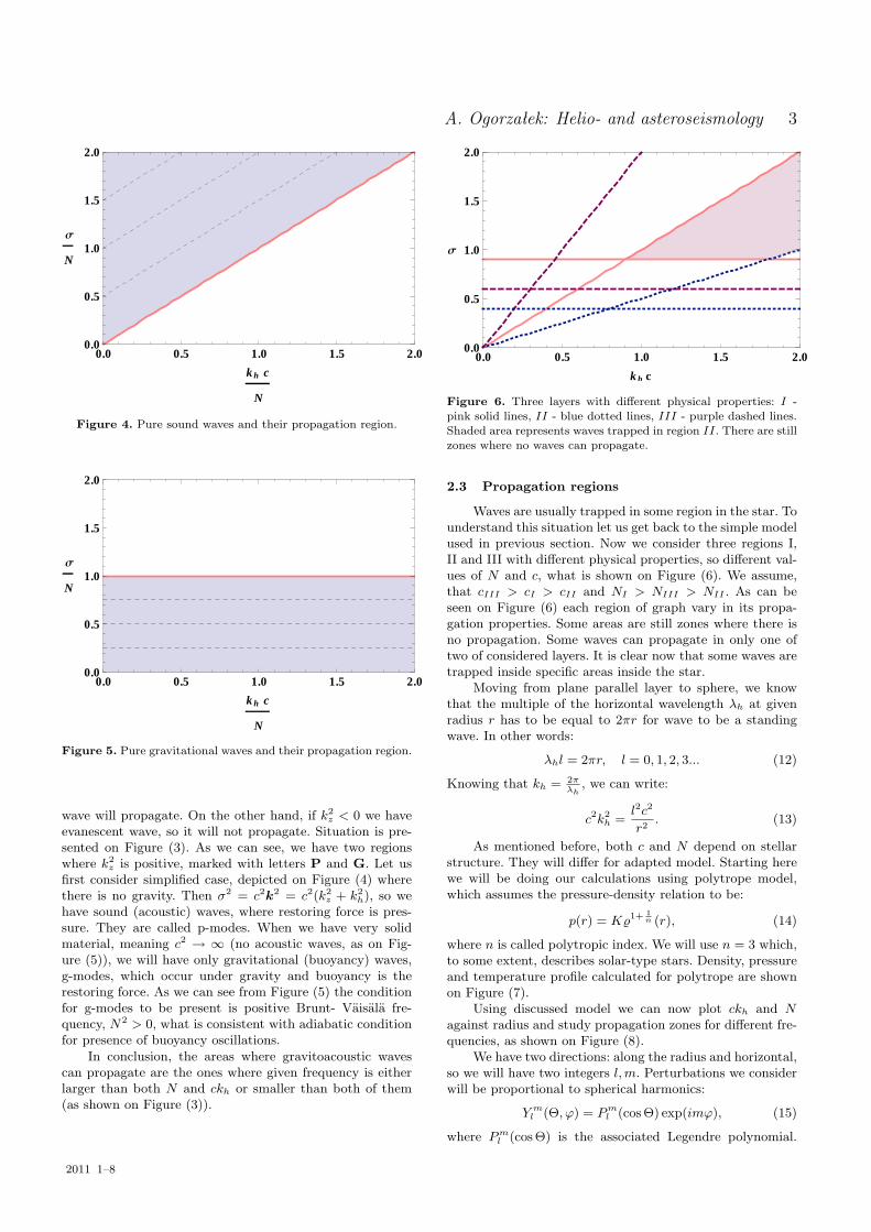
Figure 3. Relation of dispersion. Two asymptotes are depictedas dashed lines. For wave to propagate its frequency has to belarger than both N and khc, or smaller than both of them atthe same time. Shaded areas correspond to k2

z > 0. Top area iswhere pressure waves propagate (p-modes), bottom one is wheregravitational waves propagate (g-modes).

density are then connected by adiabatic relation:

δp

p0= γ

δ%

%0. (8)

γ is constant for given gas, γ = 53 for ideal gas.

Applying perturbation and adiabatic relation to equa-tions (1), (2) and (3) as well as using theoretical model(specific forms of %, p and other thermodynamic quantities)will make it possible to describe pulsations (for givenmodel).

2.2 Relation of dispersion

Let us now consider very simple model of plane isother-mal atmosphere with constant gravity force (acting alongz axis with acceleration g). Then pressure and density willchange as:

p0, %0 ∝ exp(− z

H) (9)

where H is the constant scale height. Hydrodynamics equa-tions with adiabatic approximation lead to perturbations ofthe form of:

v, p′, %′ ∝ exp(z

2H) exp(k · x), (10)

where k is a wave vector and σ is a frequency. In this situ-ation we can separate wave into horizontal coordinates andpart that propagates along the z axis, k = (kh, kz). Usingequations presented in previous section we can derive thedispersion relation between frequency and wavenumbers:

(σ2 − σ2ac)σ

2 − (k2h + k2

z)c2σ2 + k2

hc2N2 = 0. (11)

Here c2 = γ p%

is the sound speed, σac = c2H is the acoustic

cut-off frequency and N2 = −g( d ln %dr− 1γd ln pdr

) is the Brunt-Vaisala frequency.

For given σ and kh above relation determines k2z , what

allows us to describe vertical propagation of wave. If k2z > 0

2011 1–8


0.0 0.5 1.0 1.5 2.00.0

0.5

1.0

1.5

2.0

kh c

N

Σ

N

Figure 4. Pure sound waves and their propagation region.

0.0 0.5 1.0 1.5 2.00.0

0.5

1.0

1.5

2.0

kh c

N

Σ

N

Figure 5. Pure gravitational waves and their propagation region.

wave will propagate. On the other hand, if k2z < 0 we have

evanescent wave, so it will not propagate. Situation is pre-sented on Figure (3). As we can see, we have two regionswhere k2

z is positive, marked with letters P and G. Let usfirst consider simplified case, depicted on Figure (4) wherethere is no gravity. Then σ2 = c2k2 = c2(k2

z + k2h), so we

have sound (acoustic) waves, where restoring force is pres-sure. They are called p-modes. When we have very solidmaterial, meaning c2 → ∞ (no acoustic waves, as on Fig-ure (5)), we will have only gravitational (buoyancy) waves,g-modes, which occur under gravity and buoyancy is therestoring force. As we can see from Figure (5) the conditionfor g-modes to be present is positive Brunt- Vaisala fre-quency, N2 > 0, what is consistent with adiabatic conditionfor presence of buoyancy oscillations.

In conclusion, the areas where gravitoacoustic wavescan propagate are the ones where given frequency is eitherlarger than both N and ckh or smaller than both of them(as shown on Figure (3)).

0.0 0.5 1.0 1.5 2.00.0

0.5

1.0

1.5

2.0

kh c

Σ

Figure 6. Three layers with different physical properties: I -pink solid lines, II - blue dotted lines, III - purple dashed lines.Shaded area represents waves trapped in region II. There are stillzones where no waves can propagate.

2.3 Propagation regions

Waves are usually trapped in some region in the star. Tounderstand this situation let us get back to the simple modelused in previous section. Now we consider three regions I,II and III with different physical properties, so different val-ues of N and c, what is shown on Figure (6). We assume,that cIII > cI > cII and NI > NIII > NII . As can beseen on Figure (6) each region of graph vary in its propa-gation properties. Some areas are still zones where there isno propagation. Some waves can propagate in only one oftwo of considered layers. It is clear now that some waves aretrapped inside specific areas inside the star.

Moving from plane parallel layer to sphere, we knowthat the multiple of the horizontal wavelength λh at givenradius r has to be equal to 2πr for wave to be a standingwave. In other words:

λhl = 2πr, l = 0, 1, 2, 3... (12)

Knowing that kh = 2πλh

, we can write:

c2k2h =

l2c2

r2 . (13)

As mentioned before, both c and N depend on stellarstructure. They will differ for adapted model. Starting herewe will be doing our calculations using polytrope model,which assumes the pressure-density relation to be:

p(r) = K%1+ 1n (r), (14)

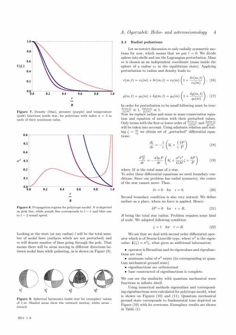
where n is called polytropic index. We will use n = 3 which,to some extent, describes solar-type stars. Density, pressureand temperature profile calculated for polytrope are shownon Figure (7).

Using discussed model we can now plot ckh and Nagainst radius and study propagation zones for different fre-quencies, as shown on Figure (8).

We have two directions: along the radius and horizontal,so we will have two integers l,m. Perturbations we considerwill be proportional to spherical harmonics:

Y ml (Θ, ϕ) = Pml (cos Θ) exp(imϕ), (15)

where Pml (cos Θ) is the associated Legendre polynomial.

2011 1–8


0.0 0.2 0.4 0.6 0.8 1.00.0

0.2

0.4

0.6

0.8

1.0

r

R

f @ fc D

Figure 7. Density (blue), pressure (purple) and temperature(pink) functions inside star, for polytrope with index n = 3 inunits of their maximum value.

0.0 0.2 0.4 0.6 0.8 1.00.0

0.1

0.2

0.3

0.4

0.5

0.6

r

R

Σ2

Figure 8. Propagation regions for polytrope model.N is depictedas pink line, while purple line corresponds to l = 1 and blue oneto l = 2 sound speed.

Looking at the start (at any radius) l will be the total num-ber of nodal lines (surfaces which are not perturbed) andm will denote number of lines going through the pole. Thatmeans there will be areas moving in different directions be-tween nodal lines while pulsating, as is shown on Figure (9).

Figure 9. Spherical harmonics inside star for exemplary valuesof l,m. Shaded areas show the outward motion, white areas -inward.

2.4 Radial pulsations

Let us restrict discussion to only radially symmetric mo-tions for now, which means that we put l = 0. We dividesphere into shells and use the Lagrangian perturbation. Massm is chosen as an independent coordinate (mass inside thesphere of a radius r0 in the equilibrium state). Applyingperturbation to radius and density leads to:

r(m, t) = r0(m) + δr(m, t) = r0(m)

(1 +

δr(m, t)r0(m)

), (16)

%(m, t) = %0(m) + δ%(m, t) = %0(m)

(1 +

δ%(m, t)%0(m)

). (17)

In order for perturbation to be small following must be true:δr(m,t)r0(m) � 1, δ%(m,t)

%0(m) � 1.Now we replace radius and mass in mass conservation equa-tion and equation of motion with their perturbed values.Only terms with the first or lower order of δr(m,t)

r0(m) and δ%(m,t)%0(m)

will be taken into account. Using adiabatic relation and stat-ing ζ = δr

r0we obtain set of „perturbed” differential equa-

tions:

dζ

dr= −1

r

(3ζ +

1γ

δP

P

)(18)

d δPP

dr= −d lnP

dr

(4ζ +

σ2r3

GMζ +

δP

P

)(19)

where M is the total mass of a star.To solve these differential equations we need boundary con-ditions. Since our problem has radial symmetry, the centerof the star cannot move. Thus:

δr = 0 for r = 0. (20)

Second boundary condition is also very natural. We definesurface as a place, where no force is applied. Hence:

δP = 0 for r = R, (21)

R being the total star radius. Problem requires some kindof scale. We adapted following condition:

ζ = 1 for r = R. (22)

We see that we deal with second order differential oper-ator which is of Sturm-Liouville type, where σ2 is the eigen-value: L(ζ) = σ2ζ, what gives us additional information:

• operator is Hermitian and its eigenvalues and eigenfunc-tions are real• minimum value of σ2 exists (its corresponding to quan-

tum mechanical ground state)• eigenfunctions are orthonormal• base constructed of eigenfunctions is complete.

We can see the similarity with quantum mechanical wavefunctions in infinite dwell.

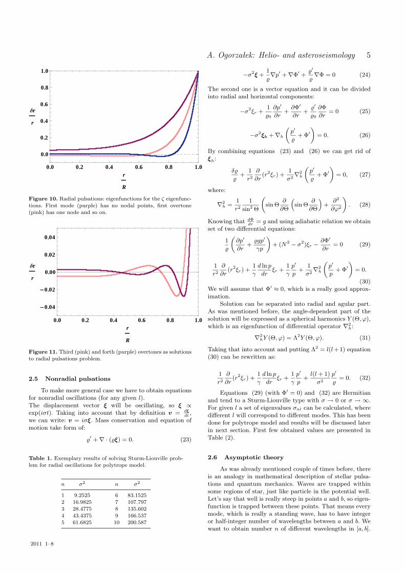
Using numerical methods eigenvalues and correspond-ing eigenfunctions were calculated for polytrope model, whatis shown on Figures (10) and (11). Quantum mechanicalground state corresponds to fundamental tone depicted onFigure (10) with its overtones. Exemplary results are shownin Table (1).

2011 1–8


0.0 0.2 0.4 0.6 0.8 1.0

0.0

0.2

0.4

0.6

0.8

1.0

r

R

∆r

r

Figure 10. Radial pulsations: eigenfunctions for the ζ eigenfunc-tions. First mode (purple) has no nodal points, first overtone(pink) has one node and so on.

0.0 0.2 0.4 0.6 0.8 1.0

-0.04

-0.02

0.00

0.02

0.04

r

R

∆r

r

Figure 11. Third (pink) and forth (purple) overtones as solutionsto radial pulsations problem.

2.5 Nonradial pulsations

To make more general case we have to obtain equationsfor nonradial oscillations (for any given l).The displacement vector ξ will be oscillating, so ξ ∝exp(iσt). Taking into account that by definition v = dξ

dt,

we can write: v = iσξ. Mass conservation and equation ofmotion take form of:

%′ +∇ · (%ξ) = 0. (23)

Table 1. Exemplary results of solving Sturm-Liouville prob-lem for radial oscillations for polytrope model.

n σ2 n σ2

1 9.2525 6 83.15252 16.9825 7 107.7973 28.4775 8 135.6024 43.4375 9 166.5375 61.6825 10 200.587

−σ2ξ +1%∇p′ +∇Φ′ +

%′

%∇Φ = 0 (24)

The second one is a vector equation and it can be dividedinto radial and horizontal components:

−σ2ξr +1%0

∂p′

∂r+∂Φ′

∂r+%′

%0

∂Φ∂r

= 0 (25)

−σ2ξh +∇h(p′

%+ Φ′

)= 0. (26)

By combining equations (23) and (26) we can get rid ofξh:

δ%

%+

1r2

∂

∂r(r2ξr) +

1σ2∇

2h

(p′

%+ Φ′

)= 0, (27)

where:

∇2h =

1r2

1sin2 Θ

(sin Θ

∂

∂Θ

(sin Θ

∂

∂Θ

)+

∂2

∂ϕ2

). (28)

Knowing that dΦdr

= g and using adiabatic relation we obtainset of two differential equations:

1%

(∂p′

∂r+%gp′

γp

)+ (N2 − σ2)ξr −

∂Φ′

∂r= 0 (29)

1r2

∂

∂r(r2ξr) +

1γ

d ln pdr

ξr +1γ

p′

p+

1σ2∇

2h

(p′

p+ Φ′

)= 0.

(30)We will assume that Φ′ ≈ 0, which is a really good approx-imation.

Solution can be separated into radial and agular part.As was mentioned before, the angle-dependent part of thesolution will be expressed as a spherical harmonics Y (Θ, ϕ),which is an eigenfunction of differential operator ∇2

h:

∇2hY (Θ, ϕ) = Λ2Y (Θ, ϕ). (31)

Taking that into account and putting Λ2 = l(l+1) equation(30) can be rewritten as:

1r2

∂

∂r(r2ξr) +

1γ

d ln pdr

ξr +1γ

p′

p+l(l + 1)σ2

p′

%= 0. (32)

Equations (29) (with Φ′ = 0) and (32) are Hermitianand tend to a Sturm-Liouville type with σ → 0 or σ → ∞.For given l a set of eigenvalues σnl can be calculated, wheredifferent l will correspond to different modes. This has beendone for polytrope model and results will be discussed laterin next section. First few obtained values are presented inTable (2).

2.6 Asymptotic theory

As was already mentioned couple of times before, thereis an analogy in mathematical description of stellar pulsa-tions and quantum mechanics. Waves are trapped withinsome regions of star, just like particle in the potential well.Let’s say that well is really steep in points a and b, so eigen-function is trapped between these points. That means everymode, which is really a standing wave, has to have integeror half-integer number of wavelengths between a and b. Wewant to obtain number n of different wavelengths in [a, b].

2011 1–8


Table 2. Exemplary results of solving Sturm-Liouville prob-lem for nonradial oscillations for polytropic model. Note thatnot all values of n are always present.

l n σ2 l n σ2

1 0 8.67961 8 0 13.22221 14.6671 1 28.90012 25.381 2 47.4353 39.5283 15 0 19.8433

2 0 9.48367 1 42.57791 17.3732 4 127.5972 29.3628 5 162.682

4 0 10.2829 30 2 110.4931 21.2265 5 245.9552 35.7032 8 412.983

0.0 0.5 1.0 1.5 2.00.0

0.5

1.0

1.5

2.0

kh c

Σ

Figure 12. Asymptotic behaviour of frequencies. For small n wehave behaviours as the pink line. For large values of n we haveblue dashed lines, pure p-modes.

Note that kr is a function of r, so we have to perform inte-gration: ∫ b

a

krdr = (n+12

)π. (33)

This is true for both waves in stars and quantum mechanics,where it is called Sommerfeld’s quantization condition.Remembering that kr = σ

cin the case of acoustic wave with

l = 0, we can write:

σ = π(n+12

)

(∫ b

a

dr

c

)−1

(34)

Integral in this equation for big values of n is constant. Theasymptotic relation for frequency is obtained:

σ = (n+12

)σ0. (35)

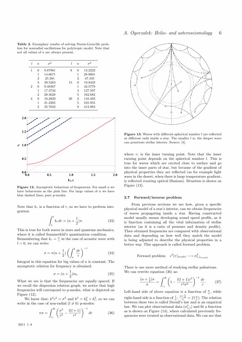
What we see is that the frequencies are equally spaced. Ifwe recall the dispersion relation graph, we notice that highfrequencies will correspond to p-modes, what is depicted onFigure (12).

We know that: k2c2 = σ2 and k2 = k2h + k2

r , so we canwrite in the case of non-radial (l 6= 0) p-modes:

nπ =

∫ R

ri

(σ2

c2− l(l + 1)

r2

)−1

dr (36)

Figure 13.Waves with different spherical number l are reflectedat different radii inside a star. The smaller l is, the deeper wavecan penetrate stellar interior. Source: [4].

where ri is the inner turning point. Note that the innerturning point depends on the spherical number l. This istrue for waves which are excited close to surface and gointo the inner parts of star, but because of the gradient ofphysical properties they are reflected (as for example lightwave in the desert, when there is large temperature gradient,is reflected creating optical illusions). Situation is shown onFigure (13).

2.7 Forward/inverse problem

From previous sections we see how, given a specificphysical model of a star’s interior, can we obtain frequenciesof waves propagating inside a star. Having constructedmodel usually means developing sound speed profile, as itis function containing all the vital information of stellarinterior (as it is a ratio of pressure and density profile).Then obtained frequencies are compared with observationaldata and depending on how well they match the modelis being adjusted to describe the physical properties in abetter way. This approach is called forward problem.

Forward problem: c2(r)model −→ σ2n,lmodel

There is one more method of studying stellar pulsations.We can rewrite equation (36) as:

(n+ 12 )π

σ=

∫ R

ri

(1− l(l + 1)c2

r2σ2

)−1dr

c. (37)

Left-hand side of above equation is a function of nσ

, while

right-hand side is a function of lσ

:n+ 12σ

= f(σl). The relation

between these two is called Duvall’s law and is an empiricallaw. We can plot observational data (σ2

n,l) and fit a functionas is shown on Figure (14), where calculated previously fre-quencies were treated as observational data. We can see that

2011 1–8


0 2 4 6 8

0.40

0.45

0.50

0.55

0.60

0.65

0.70

0.75

Σ

L H L + 1L

n + 1.5

Σ

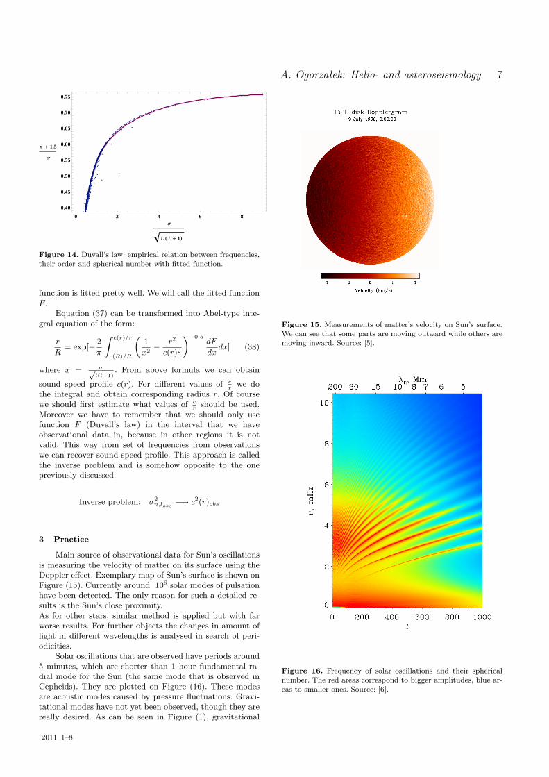
Figure 14. Duvall’s law: empirical relation between frequencies,their order and spherical number with fitted function.

function is fitted pretty well. We will call the fitted functionF .

Equation (37) can be transformed into Abel-type inte-gral equation of the form:

r

R= exp[− 2

π

∫ c(r)/r

c(R)/R

(1x2 −

r2

c(r)2

)−0.5dF

dxdx] (38)

where x = σ√l(l+1)

. From above formula we can obtain

sound speed profile c(r). For different values of cr

we dothe integral and obtain corresponding radius r. Of coursewe should first estimate what values of c

rshould be used.

Moreover we have to remember that we should only usefunction F (Duvall’s law) in the interval that we haveobservational data in, because in other regions it is notvalid. This way from set of frequencies from observationswe can recover sound speed profile. This approach is calledthe inverse problem and is somehow opposite to the onepreviously discussed.

Inverse problem: σ2n,lobs −→ c2(r)obs

3 Practice

Main source of observational data for Sun’s oscillationsis measuring the velocity of matter on its surface using theDoppler effect. Exemplary map of Sun’s surface is shown onFigure (15). Currently around 106 solar modes of pulsationhave been detected. The only reason for such a detailed re-sults is the Sun’s close proximity.As for other stars, similar method is applied but with farworse results. For further objects the changes in amount oflight in different wavelengths is analysed in search of peri-odicities.

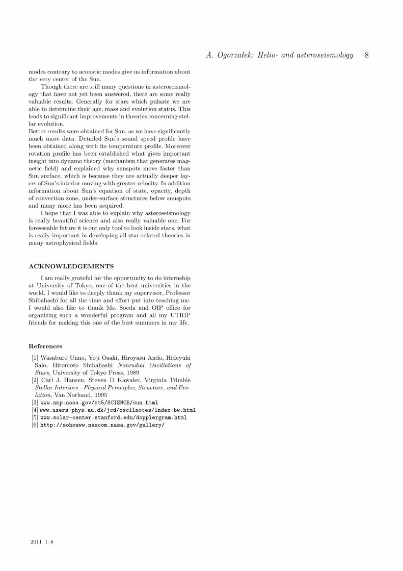
Solar oscillations that are observed have periods around5 minutes, which are shorter than 1 hour fundamental ra-dial mode for the Sun (the same mode that is observed inCepheids). They are plotted on Figure (16). These modesare acoustic modes caused by pressure fluctuations. Gravi-tational modes have not yet been observed, though they arereally desired. As can be seen in Figure (1), gravitational

Figure 15. Measurements of matter’s velocity on Sun’s surface.We can see that some parts are moving outward while others aremoving inward. Source: [5].

Figure 16. Frequency of solar oscillations and their sphericalnumber. The red areas correspond to bigger amplitudes, blue ar-eas to smaller ones. Source: [6].

2011 1–8


modes contrary to acoustic modes give us information aboutthe very center of the Sun.

Though there are still many questions in asteroseismol-ogy that have not yet been answered, there are some reallyvaluable results. Generally for stars which pulsate we areable to determine their age, mass and evolution status. Thisleads to significant improvements in theories concerning stel-lar evolution.Better results were obtained for Sun, as we have significantlymuch more data. Detailed Sun’s sound speed profile havebeen obtained along with its temperature profile. Moreoverrotation profile has been established what gives importantinsight into dynamo theory (mechanism that generates mag-netic field) and explained why sunspots move faster thanSun surface, which is because they are actually deeper lay-ers of Sun’s interior moving with greater velocity. In additioninformation about Sun’s equation of state, opacity, depthof convection zone, under-surface structures below sunspotsand many more has been acquired.

I hope that I was able to explain why asteroseismologyis really beautiful science and also really valuable one. Forforeseeable future it is our only tool to look inside stars, whatis really important in developing all star-related theories inmany astrophysical fields.

ACKNOWLEDGEMENTS

I am really grateful for the opportunity to do internshipat University of Tokyo, one of the best universities in theworld. I would like to deeply thank my supervisor, ProfessorShibahashi for all the time and effort put into teaching me.I would also like to thank Ms. Soeda and OIP office fororganizing such a wonderful program and all my UTRIPfriends for making this one of the best summers in my life.

References

[1] Wasaburo Unno, Yoji Osaki, Hiroyasu Ando, HideyukiSaio, Hiromoto Shibahashi Nonradial Oscillations ofStars, University of Tokyo Press, 1989

[2] Carl J. Hansen, Steven D Kawaler, Virginia TrimbleStellar Interiors - Physical Principles, Structure, and Evo-lution, Van Norhand, 1995

[3] www.nmp.nasa.gov/st5/SCIENCE/sun.html[4] www.users-phys.au.dk/jcd/oscilnotes/index-bw.html[5] www.solar-center.stanford.edu/dopplergram.html[6] http://sohowww.nascom.nasa.gov/gallery/

2011 1–8

basics of helio- and asteroseismology

Documents