1

BASIC CALCULUS REFRESHER

Ismor Fischer, Ph.D. Dept. of Statistics UW-Madison

1. Introduction.

This is a very condensed and simplified version of basic calculus, which is a prerequisite for many

courses in Mathematics, Statistics, Engineering, Pharmacy, etc. It is not comprehensive, and

absolutely not intended to be a substitute for a one-year freshman course in differential and integral

calculus. You are strongly encouraged to do the included Exercises to reinforce the ideas. Important

mathematical terms are in boldface; key formulas and concepts are boxed and highlighted (). To

view a color .pdf version of this document (recommended), see http://www.stat.wisc.edu/~ifischer.

2. Exponents – Basic Definitions and Properties

For any real number base x, we define powers of x: x0 = 1, x

1 = x, x

2 = x x, x

3 = x x x, etc.

(The exception is 00, which is considered indeterminate.) Powers are also called exponents.

Examples: 50 = 1, ( 11.2)

1 = 11.2, (8.6)

2 = 8.6 8.6 = 73.96, 10

3 = 10 10 10 = 1000,

( 3)4 = ( 3) ( 3) ( 3) ( 3) = 81.

Also, we can define fractional exponents in terms of roots, such as x1/2

= x , the square root of x.

Similarly, x1/3

= 3

x , the cube root of x, x2/3

= (3x)

2

, etc. In general, we have xm/n

= (nx)

m

, i.e.,

the nth

root of x, raised to the mth

power.

Examples: 641/2

= 64 = 8, 643/2

= ( 64)3

= 83 = 512, 64

1/3 =

364 = 4, 64

2/3 = (3

64)2

= 42 = 16.

Finally, we can define negative exponents: xr =

1

xr . Thus, x

1 =

1

x1 , x

2 =

1

x2 , x

1/2 =

1

x1/2 =

1

x , etc.

Examples: 101 =

1

101 = 0.1, 7

2 =

1

72 =

1

49 , 36

1/2 =

1

36 =

1

6 , 9

5/2 =

1

( 9)5

= 1

35 =

1

243 .

Properties of Exponents

1. xa x

b = x

a+b Examples: x

3 x

2 = x

5, x

1/2 x

1/3 = x

5/6, x

3 x

1/2 = x

5/2

2. x

a

xb = x

a b Examples:

x5

x3 = x

2,

x3

x5 = x

2,

x3

x1/2 = x

5/2

3. (xa)b = x

ab Examples: (x

3)2 = x

6, (x

1/2)7 = x

7/2, (x

2/3)5/7

= x10/21

2

( 1.5, 0)

(0, 7) (2.5, 7) (–1.8, 7)

(0, 3)

Desca

rtes ~

164

0

3. Functions and Their Graphs Input x Output y

If a quantity y always depends on another quantity x in such a way that every value of x corresponds

to one and only one value of y, then we say that “y is a function of x,” written y = f (x); x is said to be

the independent variable, y is the dependent variable. (Example: “Distance traveled per hour (y)

is a function of velocity (x).”) For a given function y = f(x), the set of all ordered pairs of (x, y)-

values that algebraically satisfy its equation is called the graph of the function, and can be

represented geometrically by a collection of points in the XY-plane. (Recall that the XY-plane

consists of two perpendicular copies of the real number line – a horizontal X-axis, and a vertical

Y-axis – that intersect at a reference point (0, 0) called the origin, and which partition the plane into

four disjoint regions called quadrants. Every point P in the plane can be represented by the

ordered pair (x, y), where the first value is the x-coordinate – indicating its horizontal position

relative to the origin – and the second value is the y-coordinate – indicating its vertical position

relative to the origin. Thus, the point P(4, 7) is 4 units to right of, and 7 units up from, the origin.)

Examples: y = f (x) = 7; y = f (x) = 2x + 3; y = f (x) = x2; y = f (x) = x

1/2; y = f (x) = x

1; y = f (x) = 2

x.

The first three are examples of polynomial functions. (In particular, the first is constant, the second

is linear, the third is quadratic.) The last is an exponential function; note that x is an exponent!

Let’s consider these examples, one at a time.

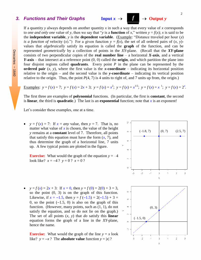
y = f (x) = 7: If x = any value, then y = 7. That is, no matter what value of x is chosen, the value of the height

y remains at a constant level of 7. Therefore, all points

that satisfy this equation must have the form (x, 7), and

thus determine the graph of a horizontal line, 7 units

up. A few typical points are plotted in the figure.

Exercise: What would the graph of the equation y = 4

look like? x = 4 ? y = 0 ? x = 0 ?

y = f (x) = 2x + 3: If x = 0, then y = f (0) = 2(0) + 3 = 3, so the point (0, 3) is on the graph of this function.

Likewise, if x = 1.5, then y = f ( 1.5) = 2( 1.5) + 3 =

0, so the point ( 1.5, 0) is also on the graph of this function. (However, many points, such as (1, 1), do not

satisfy the equation, and so do not lie on the graph.)

The set of all points (x, y) that do satisfy this linear

equation forms the graph of a line in the XY-plane,

hence the name.

Exercise: What would the graph of the line y = x look

like? y = x ? The absolute value function y = |x| ?

f

3

y = x

y = x2

Notice that the line has the generic equation y = f (x) = mx + b , where b is the Y-intercept (in this

example, b = +3), and m is the slope of the line (in this example, m = +2). In general, the slope of

any line is defined as the ratio of “height change” y to “length change” x, that is,

m = y

x =

y2 y1

x2 x1

for any two points (x1, y1) and (x2, y2) that lie on the line. For example, for the two points (0, 3) and

( 1.5, 0) on our line, the slope is m = y

x =

0 3

1.5 0 = 2, which confirms our observation.

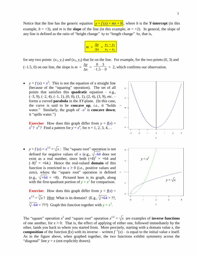
y = f (x) = x2: This is not the equation of a straight line

(because of the “squaring” operation). The set of all

points that satisfies this quadratic equation – e.g.,

(–3, 9), (–2, 4), (–1, 1), (0, 0), (1, 1), (2, 4), (3, 9), etc. –

forms a curved parabola in the XY-plane. (In this case,

the curve is said to be concave up, i.e., it “holds

water.” Similarly, the graph of –x2 is concave down;

it “spills water.”)

Exercise: How does this graph differ from y = f(x) =

x3 ? x

4 ? Find a pattern for y = x

n, for n = 1, 2, 3, 4,…

y = f (x) = x1/2

= x : The “square root” operation is not

defined for negative values of x (e.g., –64 does not exist as a real number, since both (+8)

2 = +64 and

(–8)2 = +64.) Hence the real-valued domain of this

function is restricted to x 0 (i.e., positive values and zero), where the “square root” operation is defined

(e.g., +64 = +8). Pictured here is its graph, along with the first-quadrant portion of y = x

2 for comparison.

Exercise: How does this graph differ from y = f(x) =

x1/3

= 3

x ? Hint: What is its domain? (E.g., 3

+64 = ??, 3

–64 = ???) Graph this function together with y = x3.

The “square” operation x2 and “square root” operation x

1/2 = x are examples of inverse functions

of one another, for x 0. That is, the effect of applying of either one, followed immediately by the other, lands you back to where you started from. More precisely, starting with a domain value x, the

composition of the function f(x) with its inverse – written f –1

(x) – is equal to the initial value x itself.

As in the figure above, when graphed together, the two functions exhibit symmetry across the

“diagonal” line y = x (not explicitly drawn).

4

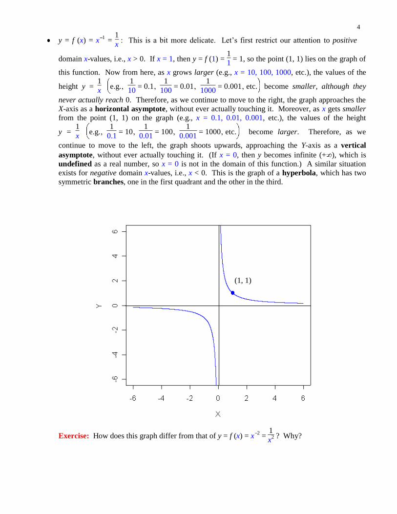
y = f (x) = x1 =

1

x : This is a bit more delicate. Let’s first restrict our attention to positive

domain x-values, i.e., x > 0. If x = 1, then y = f (1) = 1

1 = 1, so the point (1, 1) lies on the graph of

this function. Now from here, as x grows larger (e.g., x = 10, 100, 1000, etc.), the values of the

height y = 1

x e.g.‚

1

10 = 0.1‚

1

100 = 0.01‚

1

1000 = 0.001‚ etc. become smaller, although they

never actually reach 0. Therefore, as we continue to move to the right, the graph approaches the

X-axis as a horizontal asymptote, without ever actually touching it. Moreover, as x gets smaller

from the point (1, 1) on the graph (e.g., x = 0.1, 0.01, 0.001, etc.), the values of the height

y = 1

x e.g.‚

1

0.1 = 10‚

1

0.01 = 100‚

1

0.001 = 1000‚ etc. become larger. Therefore, as we

continue to move to the left, the graph shoots upwards, approaching the Y-axis as a vertical

asymptote, without ever actually touching it. (If x = 0, then y becomes infinite (+ ), which is

undefined as a real number, so x = 0 is not in the domain of this function.) A similar situation

exists for negative domain x-values, i.e., x < 0. This is the graph of a hyperbola, which has two

symmetric branches, one in the first quadrant and the other in the third.

Exercise: How does this graph differ from that of y = f (x) = x2 =

1

x2 ? Why?

(1, 1)

5

p < 0

0 < p < 1

p = 1

y = x p

p = 0

p > 1

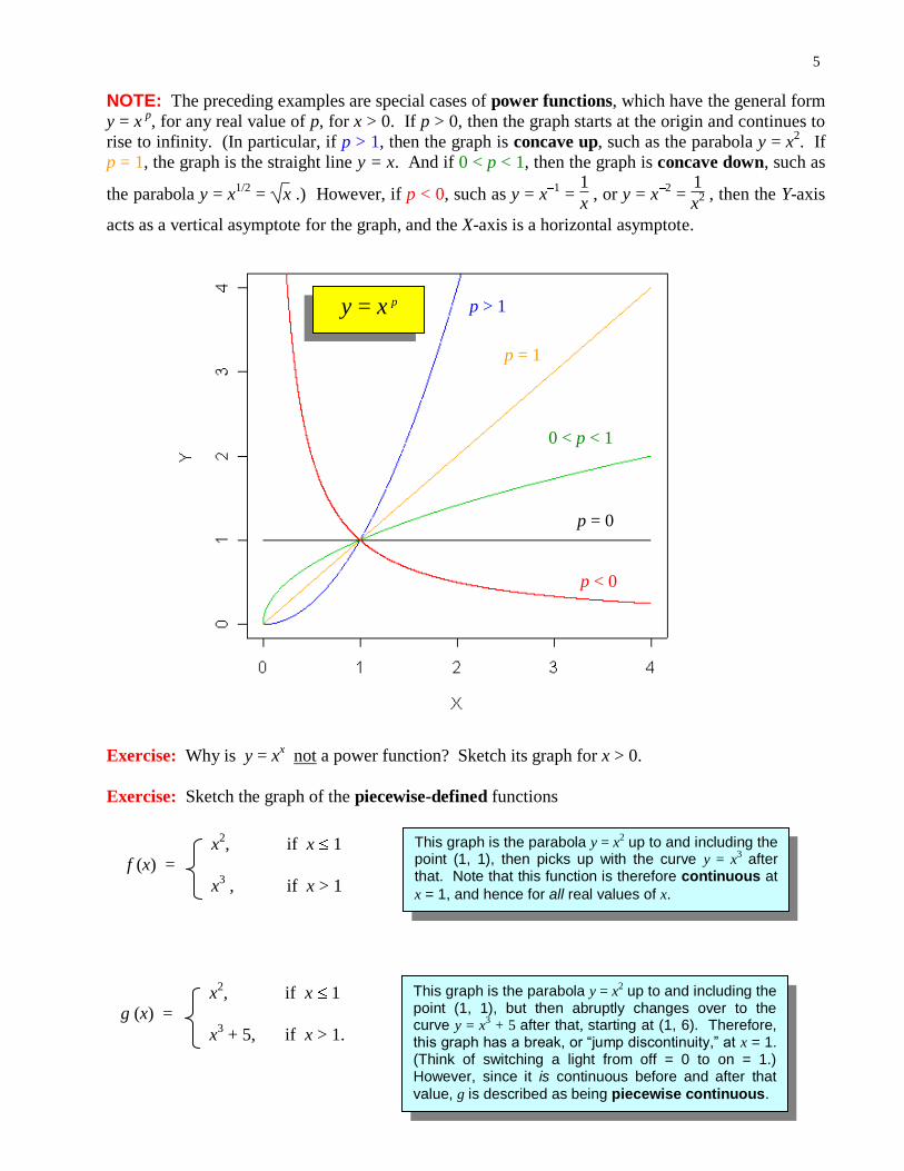
NOTE: The preceding examples are special cases of power functions, which have the general form

y = x p

, for any real value of p, for x > 0. If p > 0, then the graph starts at the origin and continues to

rise to infinity. (In particular, if p > 1, then the graph is concave up, such as the parabola y = x2. If

p = 1, the graph is the straight line y = x. And if 0 < p < 1, then the graph is concave down, such as

the parabola y = x1/2

= x .) However, if p < 0, such as y = x1 =

1

x , or y = x

2 =

1

x2 , then the Y-axis

acts as a vertical asymptote for the graph, and the X-axis is a horizontal asymptote.

Exercise: Why is y = xx not a power function? Sketch its graph for x > 0.

Exercise: Sketch the graph of the piecewise-defined functions

x2, if x 1

f (x) =

x3 , if x > 1

This graph is the parabola y = x2 up to and including the

point (1, 1), then picks up with the curve y = x3 after

that. Note that this function is therefore continuous at

x = 1, and hence for all real values of x.

x2, if x 1

g (x) =

x3 + 5, if x > 1.

This graph is the parabola y = x2 up to and including the

point (1, 1), but then abruptly changes over to the curve y = x

3 + 5 after that, starting at (1, 6). Therefore,

this graph has a break, or “jump discontinuity,” at x = 1. (Think of switching a light from off = 0 to on = 1.) However, since it is continuous before and after that

value, g is described as being piecewise continuous.

6

y = ex

y = ln(x)

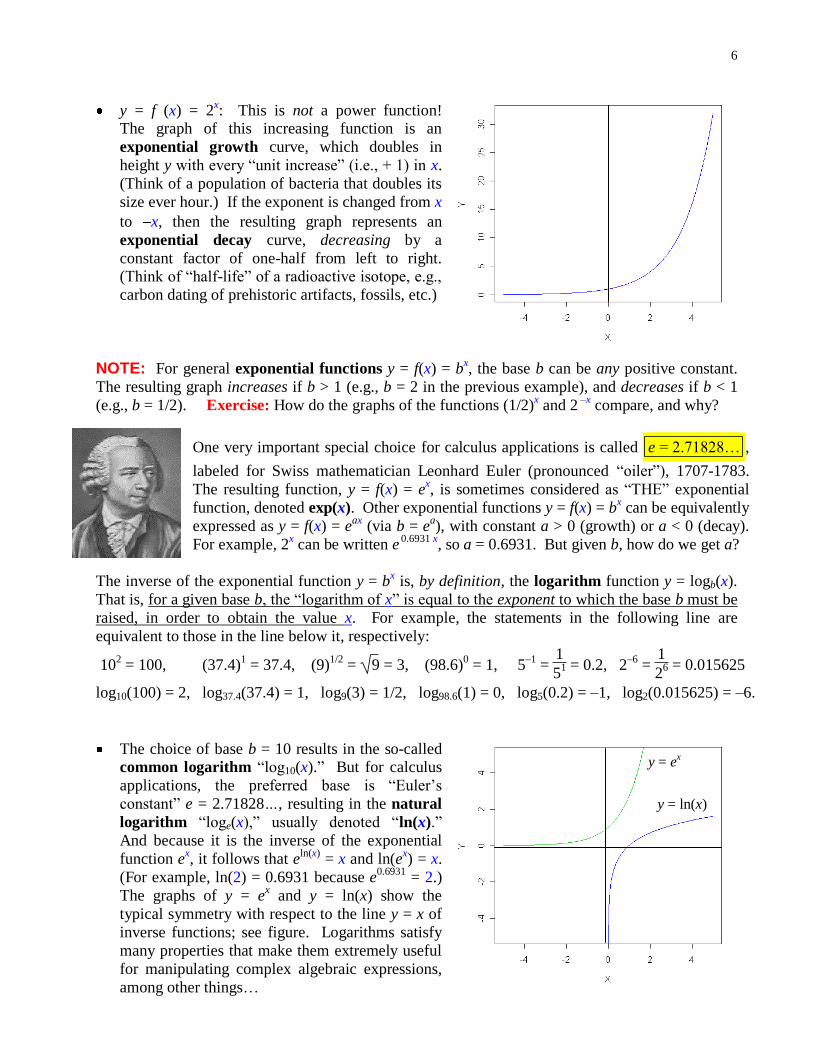
y = f (x) = 2x: This is not a power function!

The graph of this increasing function is an

exponential growth curve, which doubles in

height y with every “unit increase” (i.e., + 1) in x.

(Think of a population of bacteria that doubles its

size ever hour.) If the exponent is changed from x

to x, then the resulting graph represents an

exponential decay curve, decreasing by a

constant factor of one-half from left to right. (Think of “half-life” of a radioactive isotope, e.g.,

carbon dating of prehistoric artifacts, fossils, etc.)

NOTE: For general exponential functions y = f(x) = b

x, the base b can be any positive constant.

The resulting graph increases if b > 1 (e.g., b = 2 in the previous example), and decreases if b < 1

(e.g., b = 1/2). Exercise: How do the graphs of the functions (1/2)x and 2

–x compare, and why?

One very important special choice for calculus applications is called e = 2.71828… ,

labeled for Swiss mathematician Leonhard Euler (pronounced “oiler”), 1707-1783.

The resulting function, y = f(x) = ex, is sometimes considered as “THE” exponential

function, denoted exp(x). Other exponential functions y = f(x) = bx can be equivalently

expressed as y = f(x) = eax

(via b = ea), with constant a > 0 (growth) or a < 0 (decay).

For example, 2x can be written e 0.6931 x

, so a = 0.6931. But given b, how do we get a?

The inverse of the exponential function y = bx is, by definition, the logarithm function y = logb(x).

That is, for a given base b, the “logarithm of x” is equal to the exponent to which the base b must be

raised, in order to obtain the value x. For example, the statements in the following line are

equivalent to those in the line below it, respectively:

102 = 100, (37.4)

1 = 37.4, (9)

1/2 = 9 = 3, (98.6)

0 = 1, 5

–1 =

1

51 = 0.2, 2

–6 =

1

26 = 0.015625

log10(100) = 2, log37.4(37.4) = 1, log9(3) = 1/2, log98.6(1) = 0, log5(0.2) = –1, log2(0.015625) = –6.

The choice of base b = 10 results in the so-called common logarithm “log10(x).” But for calculus

applications, the preferred base is “Euler’s

constant” e = 2.71828…, resulting in the natural

logarithm “loge(x),” usually denoted “ln(x).”

And because it is the inverse of the exponential

function ex, it follows that e

ln(x) = x and ln(e

x) = x.

(For example, ln(2) = 0.6931 because e0.6931

= 2.)

The graphs of y = ex and y = ln(x) show the

typical symmetry with respect to the line y = x of

inverse functions; see figure. Logarithms satisfy

many properties that make them extremely useful

for manipulating complex algebraic expressions,

among other things…

7

New

ton

, Le

ibn

iz ~

16

80

4. Limits and Derivatives

We saw above that as the values of x grow ever larger, the values of 1

x become ever smaller.

We can’t actually reach 0 exactly, but we can “sneak up” on it, forcing 1

x to become as close to 0 as

we like, simply by making x large enough. (For instance, we can force 1/x < 10500

by making

x > 10500

.) In this context, we say that 0 is a limiting value of the 1

x values, as x gets arbitrarily

large. A mathematically concise way to express this is a “limit statement”:

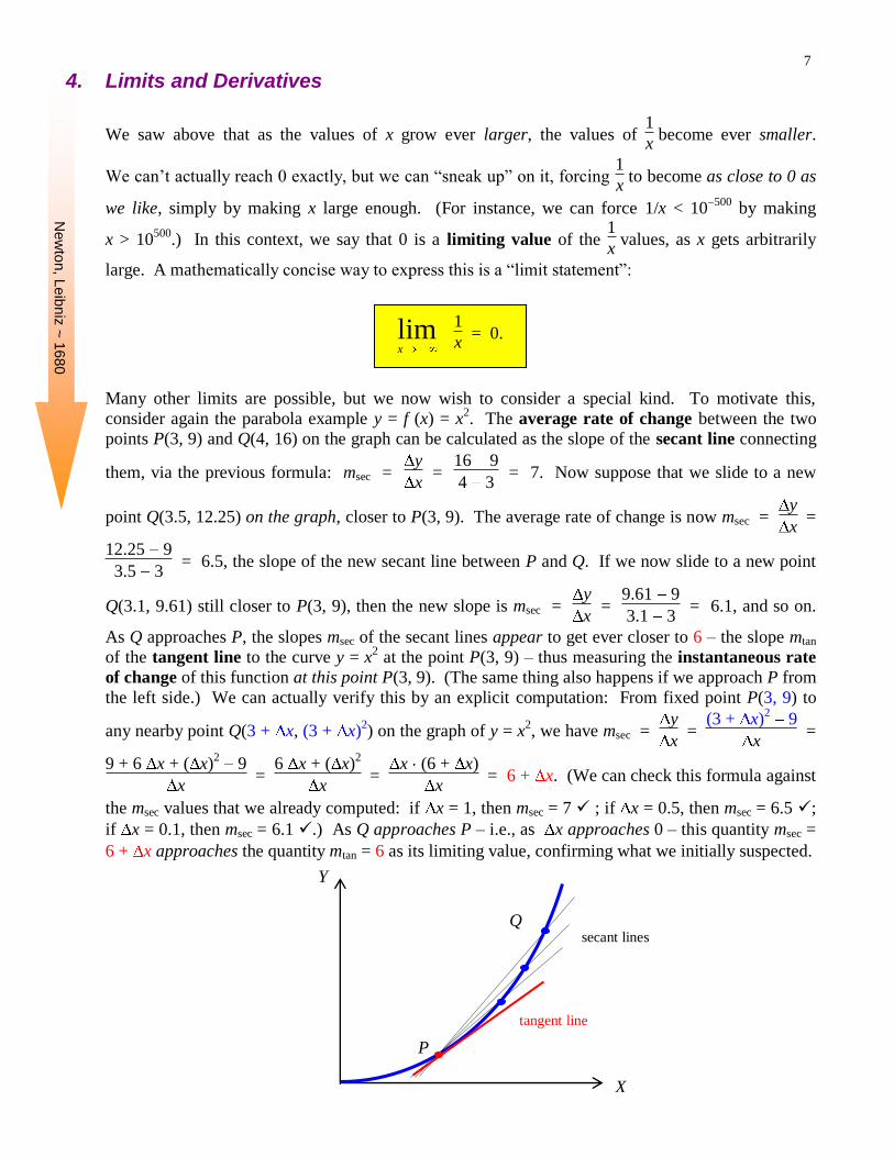
Many other limits are possible, but we now wish to consider a special kind. To motivate this,

consider again the parabola example y = f (x) = x2. The average rate of change between the two

points P(3, 9) and Q(4, 16) on the graph can be calculated as the slope of the secant line connecting

them, via the previous formula: msec = y

x =

16 9

4 3 = 7. Now suppose that we slide to a new

point Q(3.5, 12.25) on the graph, closer to P(3, 9). The average rate of change is now msec = y

x =

12.25 9

3.5 3 = 6.5, the slope of the new secant line between P and Q. If we now slide to a new point

Q(3.1, 9.61) still closer to P(3, 9), then the new slope is msec = y

x =

9.61 9

3.1 3 = 6.1, and so on.

As Q approaches P, the slopes msec of the secant lines appear to get ever closer to 6 – the slope mtan

of the tangent line to the curve y = x2 at the point P(3, 9) – thus measuring the instantaneous rate

of change of this function at this point P(3, 9). (The same thing also happens if we approach P from

the left side.) We can actually verify this by an explicit computation: From fixed point P(3, 9) to

any nearby point Q(3 + x, (3 + x)2) on the graph of y = x

2, we have msec =

y

x =

(3 + x)2 9

x =

9 + 6 x + ( x)2 9

x =

6 x + ( x)2

x =

x (6 + x)

x = 6 + x. (We can check this formula against

the msec values that we already computed: if x = 1, then msec = 7 ; if x = 0.5, then msec = 6.5 ;

if x = 0.1, then msec = 6.1 .) As Q approaches P – i.e., as x approaches 0 – this quantity msec =

6 + x approaches the quantity mtan = 6 as its limiting value, confirming what we initially suspected.

lim 1

x = 0.

x

X

Y

P

Q

tangent line

secant lines

8

X

Y

P(0, 0), mtan = 0

P(3, 9), mtan = 6

P(4, 16), mtan = 8

P( 2, 4), mtan = 4

P( 5, 25), mtan = 10

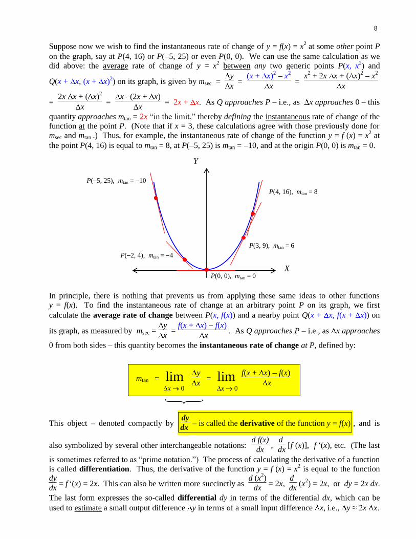
Suppose now we wish to find the instantaneous rate of change of y = f(x) = x2 at some other point P

on the graph, say at P(4, 16) or P( 5, 25) or even P(0, 0). We can use the same calculation as we

did above: the average rate of change of y = x2 between any two generic points P(x, x

2) and

Q(x + x, (x + x)2) on its graph, is given by msec =

y

x =

(x + x)2 x

2

x =

x2 + 2x x + ( x)

2 x

2

x

= 2x x + ( x)

2

x =

x (2x + x)

x = 2x + x. As Q approaches P – i.e., as x approaches 0 – this

quantity approaches mtan = 2x “in the limit,” thereby defining the instantaneous rate of change of the

function at the point P. (Note that if x = 3, these calculations agree with those previously done for

msec and mtan .) Thus, for example, the instantaneous rate of change of the function y = f (x) = x2 at

the point P(4, 16) is equal to mtan = 8, at P( 5, 25) is mtan = 10, and at the origin P(0, 0) is mtan = 0.

In principle, there is nothing that prevents us from applying these same ideas to other functions

y = f(x). To find the instantaneous rate of change at an arbitrary point P on its graph, we first

calculate the average rate of change between P(x, f(x)) and a nearby point Q(x + x, f(x + x)) on

its graph, as measured by msec = y

x =

f(x + x) f(x)

x . As Q approaches P – i.e., as x approaches

0 from both sides – this quantity becomes the instantaneous rate of change at P, defined by:

This object – denoted compactly by dy

dx – is called the derivative of the function y = f(x) , and is

also symbolized by several other interchangeable notations: d f(x)

dx ,

d

dx [f (x)], f (x), etc. (The last

is sometimes referred to as “prime notation.”) The process of calculating the derivative of a function

is called differentiation. Thus, the derivative of the function y = f (x) = x2 is equal to the function

dy

dx = f (x) = 2x. This can also be written more succinctly as

d (x2)

dx = 2x,

d

dx (x

2) = 2x, or dy = 2x dx.

The last form expresses the so-called differential dy in terms of the differential dx, which can be

used to estimate a small output difference y in terms of a small input difference x, i.e., y ≈ 2x x.

mtan = lim y

x = lim

f(x + x) f(x)

x

x 0 x 0

9

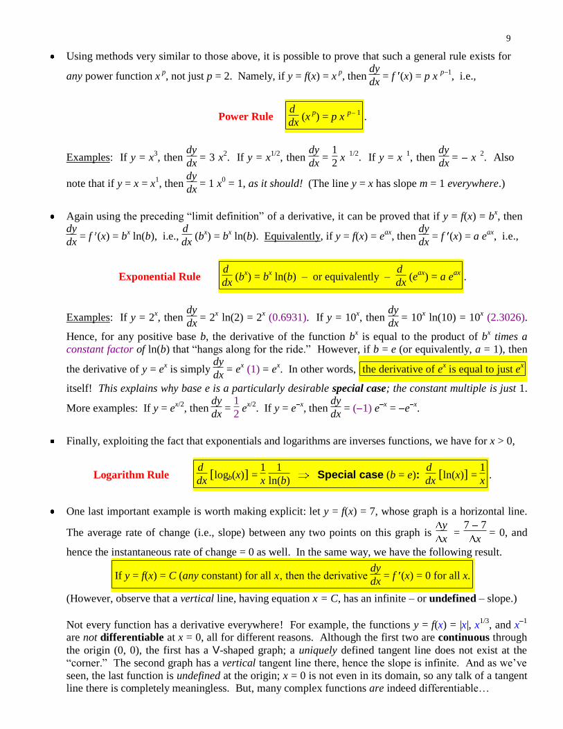
Using methods very similar to those above, it is possible to prove that such a general rule exists for

any power function x p, not just p = 2. Namely, if y = f(x) = x

p, then

dy

dx = f (x) = p x

p 1, i.e.,

Power Rule d

dx (x

p) = p x

p 1.

Examples: If y = x3, then

dy

dx = 3 x

2. If y = x

1/2, then

dy

dx =

1

2 x

1/2. If y = x

1, then

dy

dx = x

2. Also

note that if y = x = x1, then

dy

dx = 1 x

0 = 1, as it should! (The line y = x has slope m = 1 everywhere.)

Again using the preceding “limit definition” of a derivative, it can be proved that if y = f(x) = bx, then

dy

dx = f (x) = b

x ln(b), i.e.,

d

dx (b

x) = b

x ln(b). Equivalently, if y = f(x) = e

ax, then

dy

dx = f (x) = a e

ax, i.e.,

Exponential Rule d

dx (b

x) = b

x ln(b) – or equivalently –

d

dx (e

ax) = a e

ax.

Examples: If y = 2x, then

dy

dx = 2

x ln(2) = 2

x (0.6931). If y = 10

x, then

dy

dx = 10

x ln(10) = 10

x (2.3026).

Hence, for any positive base b, the derivative of the function bx is equal to the product of b

x times a

constant factor of ln(b) that “hangs along for the ride.” However, if b = e (or equivalently, a = 1), then

the derivative of y = ex is simply

dy

dx = e

x (1) = e

x. In other words, the derivative of e

x is equal to just e

x

itself! This explains why base e is a particularly desirable special case; the constant multiple is just 1.

More examples: If y = ex/2

, then dy

dx =

1

2 e

x/2. If y = e

x, then

dy

dx = ( 1) e

x = e

x.

Finally, exploiting the fact that exponentials and logarithms are inverses functions, we have for x > 0,

Logarithm Rule d

dx [logb(x)] =

1

x

1

ln(b) Special case (b = e):

d

dx [ln(x)] =

1

x.

One last important example is worth making explicit: let y = f(x) = 7, whose graph is a horizontal line.

The average rate of change (i.e., slope) between any two points on this graph is y

x =

7 7

x = 0, and

hence the instantaneous rate of change = 0 as well. In the same way, we have the following result.

If y = f(x) = C (any constant) for all x‚ then the derivative dy

dx = f (x) = 0 for all x.

(However, observe that a vertical line, having equation x = C, has an infinite – or undefined – slope.)

Not every function has a derivative everywhere! For example, the functions y = f(x) = |x|, x1/3

, and x1

are not differentiable at x = 0, all for different reasons. Although the first two are continuous through

the origin (0, 0), the first has a V-shaped graph; a uniquely defined tangent line does not exist at the

“corner.” The second graph has a vertical tangent line there, hence the slope is infinite. And as we’ve

seen, the last function is undefined at the origin; x = 0 is not even in its domain, so any talk of a tangent line there is completely meaningless. But, many complex functions are indeed differentiable…

10

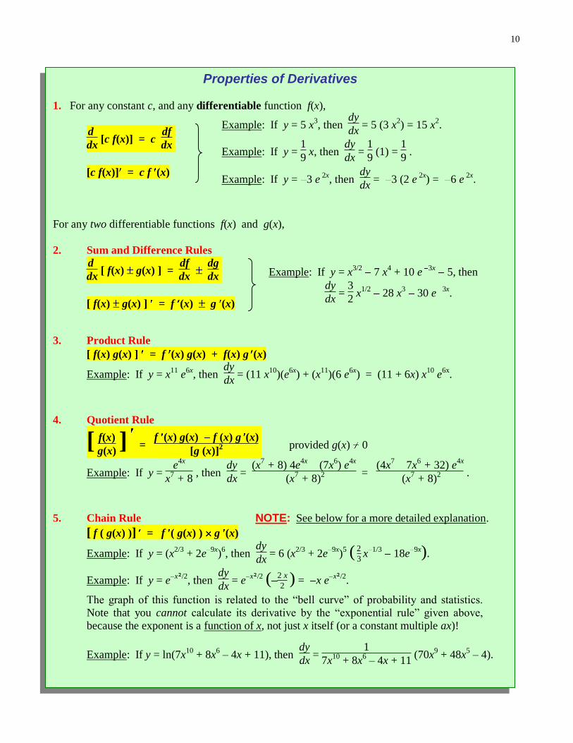
Properties of Derivatives

1. For any constant c, and any differentiable function f(x),

d

dx [c f(x)] = c

df

dx

[c f(x)] = c f (x)

For any two differentiable functions f(x) and g(x),

2. Sum and Difference Rules

d

dx [ f(x) g(x) ] =

df

dx

dg

dx

[ f(x) g(x) ] = f (x) g (x)

3. Product Rule

[ f(x) g(x) ] = f (x) g(x) + f(x) g (x)

Example: If y = x11

e6x

, then dy

dx = (11 x

10)(e

6x) + (x

11)(6 e

6x) = (11 + 6x) x

10 e

6x.

4. Quotient Rule

[ f(x)

g(x) ] =

f (x) g(x) f (x) g (x)

[g (x)]2 provided g(x) 0

Example: If y = e

4x

x7 + 8

, then dy

dx =

(x7 + 8) 4e

4x (7x

6) e

4x

(x7 + 8)

2 = (4x

7 7x

6 + 32) e

4x

(x7 + 8)

2 .

5. Chain Rule NOTE: See below for a more detailed explanation.

[ f ( g(x) )] = f ( g(x) ) g (x)

Example: If y = (x2/3

+ 2e9x

)6, then

dy

dx = 6 (x

2/3 + 2e

9x)5 (

2

3 x

1/3 18e

9x).

Example: If y = ex²/2

, then dy

dx = e

x²/2 ( 2 x

2 ) = x e

x²/2.

The graph of this function is related to the “bell curve” of probability and statistics.

Note that you cannot calculate its derivative by the “exponential rule” given above,

because the exponent is a function of x, not just x itself (or a constant multiple ax)!

Example: If y = ln(7x10

+ 8x6 – 4x + 11), then

dy

dx =

1

7x10

+ 8x6 – 4x + 11

(70x9 + 48x

5 – 4).

Example: If y = x3/2

7 x4 + 10 e

3x 5, then

dy

dx =

3

2 x

1/2 28 x

3 30 e

3x.

Example: If y = 5 x3, then

dy

dx = 5 (3 x

2) = 15 x

2.

Example: If y = 1

9 x, then

dy

dx =

1

9 (1) =

1

9 .

Example: If y = 3 e 2x

, then dy

dx = 3 (2 e

2x) = 6 e

2x.

11

The Chain Rule, which can be written several different ways, bears some further explanation. It is a

rule for differentiating a composition of two functions f and g, that is, a function of a function

y = f ( g(x) ). The function in the first example above can be viewed as composing the “outer”

function f(u) = u6, with the “inner” function u = g(x) = x

2/3 + 2e

9x. To find its derivative, first take

the derivative of the outer function (6u5, by the Power Rule given above), then multiply that by the

derivative of the inner, and we get our answer. Similarly, the function in the second example can be

viewed as composing the outer exponential function f(u) = eu (whose derivative, recall, is itself),

with the inner power function u = g(x) = x2/2. And the last case can be seen as composing the outer

logarithm function f(u) = ln(u) with the inner polynomial function u = g(x) = 7x10

+ 8x6 – 4x + 11.

Hence, if y = f(u)‚ and u = g(x)‚ then dy

dx = f (u) g

(x) is another way to express this procedure.

The logic behind the Chain Rule is actually quite simple and intuitive (though a formal proof

involves certain technicalities that we do not pursue here). Imagine three cars traveling at different

rates of speed over a given time interval: A travels at a rate of 60 mph, B travels at a rate of 40 mph,

and C travels at a rate of 20 mph. In addition, suppose that A knows how fast B is traveling, and B

knows how fast C is traveling, but A does not know how fast C is traveling. Over this time span, the

average rate of change of A, relative to B, is equal to the ratio of their respective distances traveled,

i.e., A

B =

60

40 =

3

2, three-halves as much. Similarly, the average rate of change of B, relative to C, is

equal to the ratio B

C =

40

20 =

2

1, twice as much. Therefore, the average rate of change of A, relative to

C, can be obtained by multiplying together these two quantities, via the elementary algebraic identity

A

C =

A

B

B

C , or

3

2

2

1 =

3

1, three times as much. (Of course, if A has direct knowledge of C, this

would not be necessary, for A

C =

60

20 =

3

1. As it is, B acts an intermediate link in the chain, or an

auxiliary function, which makes calculations easier in some contexts.) The idea behind the Chain

Rule is that what is true for average rates of change also holds for instantaneous rates of change, as

the time interval shrinks to 0 “in the limit,” i.e., derivatives.

With this insight, an alternate – perhaps more illuminating – equivalent way to write the Chain Rule

is dy

dx =

dy

du

du

dx which, as the last three examples illustrate, specialize to a General Power Rule,

General Exponential Rule, and General Logarithm Rule for differentiation, respectively:

Exercise: Recall from page 5 that y = xx is not a power function. Obtain its derivative via the

technique of implicit (in particular, logarithmic) differentiation. (Not covered here.)

If y = u p, then

dy

dx = p u

p 1 du

dx . That is, d(u

p) = p u

p 1 du.

If y = e u, then

dy

dx = e

u du

dx . That is, d(e

u) = e

u du.

If y = ln(u), then dy

dx =

1

u du

dx . That is, d[ln(u)] =

1

u du.

12

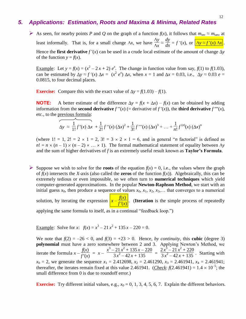
5. Applications: Estimation, Roots and Maxima & Minima, Related Rates

As seen, for nearby points P and Q on the graph of a function f(x), it follows that msec ≈ mtan, at

least informally. That is, for a small change x, we have y

x ≈

dy

dx = f (x), or y ≈ f (x) x .

Hence the first derivative f (x) can be used in a crude local estimate of the amount of change y

of the function y = f(x).

Example: Let y = f(x) = (x2 – 2 x + 2) e

x. The change in function value from say, f(1) to f(1.03),

can be estimated by y ≈ f (x) x = (x2 e

x) x, when x = 1 and x = 0.03, i.e., y ≈ 0.03 e =

0.0815, to four decimal places.

Exercise: Compare this with the exact value of y = f(1.03) – f(1).

NOTE: A better estimate of the difference y = f(x + x) – f(x) can be obtained by adding

information from the second derivative f (x) (= derivative of f (x)), the third derivative f (x),

etc., to the previous formula:

y ≈ 1

1! f (x) x +

1

2! f (x) ( x)

2 +

1

3! f (x) ( x)

3 + … +

1

n! f

(n)(x) ( x)

n

(where 1! = 1, 2! = 2 1 = 2, 3! = 3 2 1 = 6, and in general “n factorial” is defined as

n! = n (n – 1) (n – 2) … 1). The formal mathematical statement of equality between y

and the sum of higher derivatives of f is an extremely useful result known as Taylor’s Formula.

Suppose we wish to solve for the roots of the equation f(x) = 0, i.e., the values where the graph

of f(x) intersects the X-axis (also called the zeros of the function f(x)). Algebraically, this can be

extremely tedious or even impossible, so we often turn to numerical techniques which yield

computer-generated approximations. In the popular Newton-Raphson Method, we start with an

initial guess x0, then produce a sequence of values x0, x1, x2, x3,… that converges to a numerical

solution, by iterating the expression x – f(x)

f (x)

. (Iteration is the simple process of repeatedly

applying the same formula to itself, as in a continual “feedback loop.”)

Example: Solve for x: f(x) = x3 – 21 x

2 + 135 x – 220 = 0.

We note that f(2) = –26 < 0, and f(3) = +23 > 0. Hence, by continuity, this cubic (degree 3)

polynomial must have a zero somewhere between 2 and 3. Applying Newton’s Method, we

iterate the formula x – f(x)

f (x)

= x – x

3 – 21 x

2 + 135 x – 220

3 x2 – 42 x + 135

= 2 x

3 – 21 x

2 + 220

3 x2 – 42 x + 135

. Starting with

x0 = 2, we generate the sequence x1 = 2.412698, x2 = 2.461290, x3 = 2.461941, x4 = 2.461941;

thereafter, the iterates remain fixed at this value 2.461941. (Check: f(2.461941) = 1.4 10–5

; the small difference from 0 is due to roundoff error.)

Exercise: Try different initial values, e.g., x0 = 0, 1, 3, 4, 5, 6, 7. Explain the different behaviors.

13

Notice the extremely rapid convergence to the root. In fact, it can be shown that the small

error (between each value and the true solution) in each iteration is approximately squared in the

next iteration, resulting in a much smaller error. This feature of quadratic convergence is a

main reason why this is a favorite method. Why does it work at all? Suppose P0 is a point on

the graph of f(x), whose x-coordinate x0 is reasonably close to a root. Generally speaking, the

tangent line at P0 will then intersect the X-axis at a value much closer to the root. This value x1

can then be used as the x-coordinate of a new point P1 on the graph, and the cycle repeated until

some predetermined error tolerance is reached. Algebraically formalizing this process results in

the general formula given above.

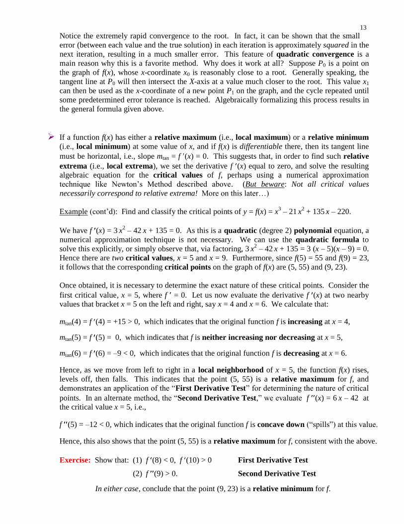
If a function f(x) has either a relative maximum (i.e., local maximum) or a relative minimum

(i.e., local minimum) at some value of x, and if f(x) is differentiable there, then its tangent line

must be horizontal, i.e., slope mtan = f (x) = 0. This suggests that, in order to find such relative

extrema (i.e., local extrema), we set the derivative f (x) equal to zero, and solve the resulting algebraic equation for the critical values of f, perhaps using a numerical approximation

technique like Newton’s Method described above. (But beware: Not all critical values

necessarily correspond to relative extrema! More on this later…)

Example (cont’d): Find and classify the critical points of y = f(x) = x3 – 21 x

2 + 135 x – 220.

We have f (x) = 3 x2 – 42 x + 135 = 0. As this is a quadratic (degree 2) polynomial equation, a

numerical approximation technique is not necessary. We can use the quadratic formula to

solve this explicitly, or simply observe that, via factoring, 3 x2 – 42 x + 135 = 3 (x – 5)(x – 9) = 0.

Hence there are two critical values, x = 5 and x = 9. Furthermore, since f(5) = 55 and f(9) = 23,

it follows that the corresponding critical points on the graph of f(x) are (5, 55) and (9, 23).

Once obtained, it is necessary to determine the exact nature of these critical points. Consider the

first critical value, x = 5, where f = 0. Let us now evaluate the derivative f (x) at two nearby values that bracket x = 5 on the left and right, say x = 4 and x = 6. We calculate that:

mtan(4) = f (4) = +15 > 0, which indicates that the original function f is increasing at x = 4,

mtan(5) = f (5) = 0, which indicates that f is neither increasing nor decreasing at x = 5,

mtan(6) = f (6) = –9 < 0, which indicates that the original function f is decreasing at x = 6.

Hence, as we move from left to right in a local neighborhood of x = 5, the function f(x) rises,

levels off, then falls. This indicates that the point (5, 55) is a relative maximum for f, and

demonstrates an application of the “First Derivative Test” for determining the nature of critical

points. In an alternate method, the “Second Derivative Test,” we evaluate f (x) = 6 x – 42 at the critical value x = 5, i.e.,

f (5) = –12 < 0, which indicates that the original function f is concave down (“spills”) at this value.

Hence, this also shows that the point (5, 55) is a relative maximum for f, consistent with the above.

Exercise: Show that: (1) f (8) < 0, f (10) > 0 First Derivative Test

(2) f (9) > 0. Second Derivative Test

In either case, conclude that the point (9, 23) is a relative minimum for f.

14

(2.461941, 0)

(5, 55)

(9, 23) (7, 39)

f decreases

f concave down f concave up

f increases f increases

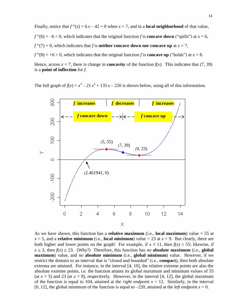
Finally, notice that f (x) = 6 x – 42 = 0 when x = 7, and in a local neighborhood of that value,

f (6) = –6 < 0, which indicates that the original function f is concave down (“spills”) at x = 6,

f (7) = 0, which indicates that f is neither concave down nor concave up at x = 7,

f (8) = +6 > 0, which indicates that the original function f is concave up (“holds”) at x = 8.

Hence, across x = 7, there is change in concavity of the function f(x). This indicates that (7, 39)

is a point of inflection for f.

The full graph of f(x) = x3 – 21 x

2 + 135 x – 220 is shown below, using all of this information.

As we have shown, this function has a relative maximum (i.e., local maximum) value = 55 at

x = 5, and a relative minimum (i.e., local minimum) value = 23 at x = 9. But clearly, there are

both higher and lower points on the graph! For example, if x 11, then f(x) 55; likewise, if

x 3, then f(x) 23. (Why?) Therefore, this function has no absolute maximum (i.e., global

maximum) value, and no absolute minimum (i.e., global minimum) value. However, if we

restrict the domain to an interval that is “closed and bounded” (i.e., compact), then both absolute

extrema are attained. For instance, in the interval [4, 10], the relative extreme points are also the

absolute extreme points, i.e. the function attains its global maximum and minimum values of 55

(at x = 5) and 23 (at x = 9), respectively. However, in the interval [4, 12], the global maximum

of the function is equal to 104, attained at the right endpoint x = 12. Similarly, in the interval

[0, 12], the global minimum of the function is equal to –220, attained at the left endpoint x = 0.

15

Exercise: Graph each of the following.

f(x) = x3 – 21 x

2 + 135 x – 243

f(x) = x3 – 21 x

2 + 135 x – 265

f(x) = x3 – 21 x

2 + 147 x – 265

Exercise: The origin (0, 0) is a critical point for both f(x) = x3 and f(x) = x

4. (Why?) Using the

tests above, formally show that it is a relative minimum of the latter, but a point of inflection

of the former. Graph both of these functions.

The volume V of a spherical cell is functionally related to its radius r via the formula V = 4

3 r

3.

Hence, the derivative dV

dr = 4 r

2 naturally expresses the instantaneous rate of change of V with

respect to r. But as V and r are functions of time, we can relate both their rates directly, by

differentiating the original relation with respect to the time variable t, yielding the equation dV

dt = 4 r

2 dr

dt. Observant readers will note that the two equations are mathematically equivalent

via the Chain Rule, since dV

dt =

dV

dr dr

dt, but the second form illustrates a simple application of a

general technique called related rates. That is, the “time derivative” of a functional relation

between two or more variables results in a type of differential equation that relates their rates.

6. Integrals and Antiderivatives

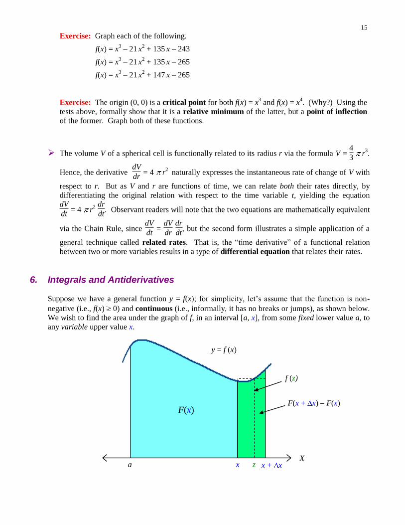
Suppose we have a general function y = f(x); for simplicity, let’s assume that the function is non-

negative (i.e., f(x) 0) and continuous (i.e., informally, it has no breaks or jumps), as shown below.

We wish to find the area under the graph of f, in an interval [a, x], from some fixed lower value a, to

any variable upper value x.

X a x x + x z

F(x + x) F(x)

f (z)

y = f (x)

F(x)

16

We formally define a new function

F(x) = Area under the graph of f in the interval [a, x].

Clearly, because every value of x results in one and only one area (shown highlighted above in blue),

this is a function of x, by definition! Moreover, F must also have a strong connection with f itself.

To see what that connection must be, consider a nearby value x + x. Then,

F(x + x) = Area under the graph of f in the interval [a, x + x],

and take the difference of these two areas (highlighted above in green):

F(x + x) F(x) = Area under the graph of f in the interval [x, x + x]

= Area of the rectangle with height f(z) and width x

(where z is some value in the interval [x, x + x])

= f(z) x.

Therefore, we have

F(x + x) F(x)

x = f(z).

Now take the limit of both sides as x 0. We see that the left hand side becomes the derivative of

F(x) (recall the definition of the derivative of a function, previously given) and, noting that z x as

x 0, we see that the right hand side f(z) becomes (via continuity) f(x). Hence,

F (x) = f(x) ,

i.e., F is an antiderivative of f.

Therefore, we formally express… F(x) =

a

x

f(t) dt ,

where the right-hand side

a

x

f(t) dt represents the definite integral of the function f from a to x.

(In this context, f is called the integrand.) More generally, if F is any antiderivative of f, then the

two functions are related via the indefinite integral: f(x) dx = F(x) + C , where C is an arbitrary

constant.

Example 1: F(x) = 1

10 x

10 + C (where C is any constant) is the general antiderivative of f(x) = x

9,

because F (x) = 1

10 (10x

9) + 0 = x

9 = f(x).

We can write this relation succinctly as x9 dx =

1

10 x

10 + C.

17

Example 2: F(x) = 8 e x/8

+ C (where C is any constant) is the general antiderivative of f(x) = e x/8

,

because F (x) = 8 (1

8 e

x/8) + 0 = e x/8

= f(x).

We can write this relation succinctly as e x/8

dx = 8 e x/8

+ C.

NOTE: Integrals possess the analogues of Properties 1 and 2 for derivatives, found on page 10. In particular, the integral of a constant multiple of a function, c f(x), is equal to that constant

multiple c, times the integral of the function f(x). Also, the integral of a sum (respectively,

difference) of two functions is equal to the sum (respectively, difference) of the integrals. (The

integral analogue for products corresponds to a technique known as integration by parts; not

reviewed here.) These are extremely important properties for the applications that follow.

From the previous two examples, it is evident that the differentiation rules for power and

exponential functions can be inverted (essentially by taking the integral of both sides) to the

General Power Rule, General Logarithm Rule, and General Exponential Rule for integration:

NOTE: In order to use these formulas correctly, du must be present in the integrand (up to a constant multiple). To illustrate…

u

p+1

p + 1 + C, if p 1

u p du =

ln |u| + C, if p = 1

eu du = e

u + C

Properties of Integrals

1. For any constant c, and any integrable function f(x),

[c f(x)] dx = c f(x) dx

For any two integrable functions f(x) and g(x),

2. Sum and Difference Rules

[f(x) g(x)] dx = f(x) dx g(x) dx

18

u1 du = ln |u| + C

du = eu + C e

u

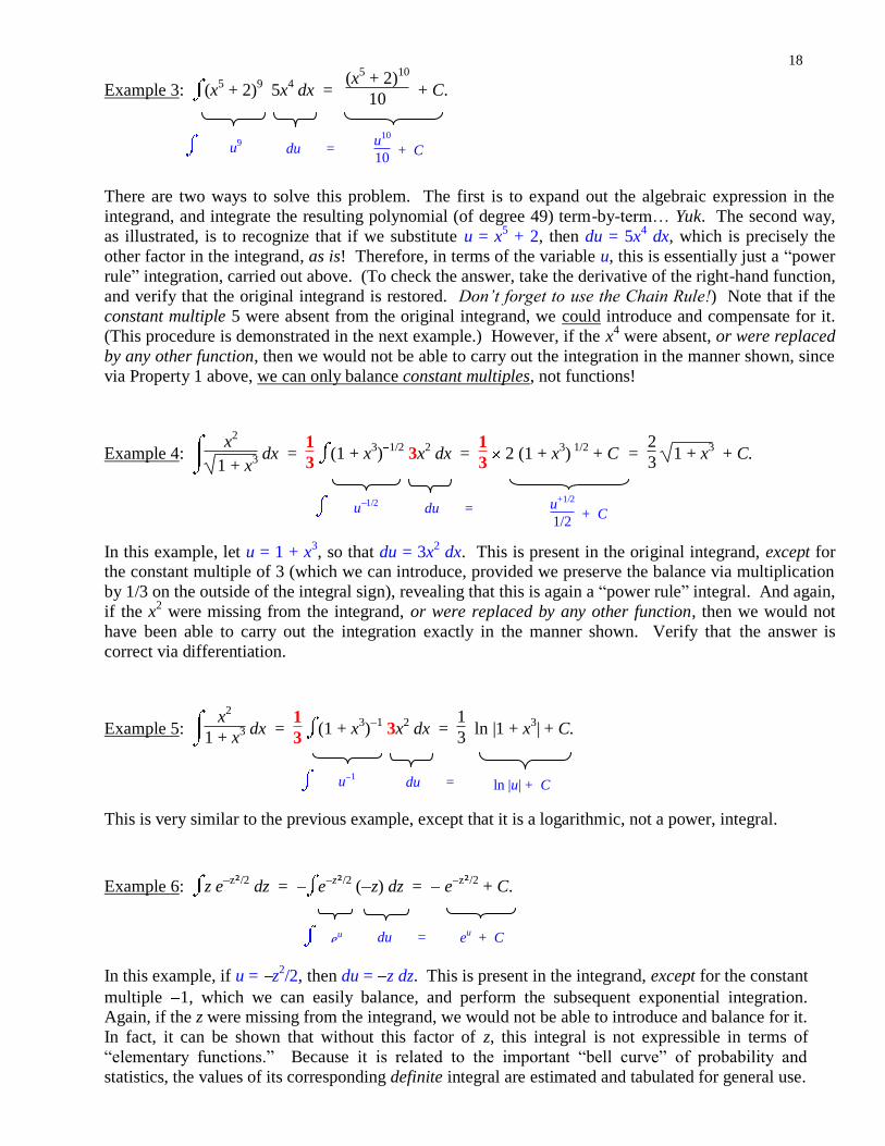
Example 3: (x5 + 2)

9 5x

4 dx =

(x5 + 2)

10

10 + C.

There are two ways to solve this problem. The first is to expand out the algebraic expression in the

integrand, and integrate the resulting polynomial (of degree 49) term-by-term… Yuk. The second way,

as illustrated, is to recognize that if we substitute u = x5 + 2, then du = 5x

4 dx, which is precisely the

other factor in the integrand, as is! Therefore, in terms of the variable u, this is essentially just a “power

rule” integration, carried out above. (To check the answer, take the derivative of the right-hand function,

and verify that the original integrand is restored. Don’t forget to use the Chain Rule!) Note that if the

constant multiple 5 were absent from the original integrand, we could introduce and compensate for it.

(This procedure is demonstrated in the next example.) However, if the x4 were absent, or were replaced

by any other function, then we would not be able to carry out the integration in the manner shown, since

via Property 1 above, we can only balance constant multiples, not functions!

Example 4: x

2

1 + x3 dx =

1

3 (1 + x

3)

1/2 3x

2 dx =

1

3 2 (1 + x

3) 1/2

+ C = 2

3 1 + x

3 + C.

In this example, let u = 1 + x3, so that du = 3x

2 dx. This is present in the original integrand, except for

the constant multiple of 3 (which we can introduce, provided we preserve the balance via multiplication

by 1/3 on the outside of the integral sign), revealing that this is again a “power rule” integral. And again,

if the x2 were missing from the integrand, or were replaced by any other function, then we would not

have been able to carry out the integration exactly in the manner shown. Verify that the answer is

correct via differentiation.

Example 5: x

2

1 + x3 dx =

1

3 (1 + x

3)

1 3x

2 dx =

1

3 ln |1 + x

3| + C.

This is very similar to the previous example, except that it is a logarithmic, not a power, integral.

Example 6: z ez²/2

dz = ez²/2

( z) dz = ez²/2

+ C.

In this example, if u = z2/2, then du = z dz. This is present in the integrand, except for the constant

multiple 1, which we can easily balance, and perform the subsequent exponential integration. Again, if the z were missing from the integrand, we would not be able to introduce and balance for it.

In fact, it can be shown that without this factor of z, this integral is not expressible in terms of

“elementary functions.” Because it is related to the important “bell curve” of probability and

statistics, the values of its corresponding definite integral are estimated and tabulated for general use.

u1/2

du = u+1/2

1/2 + C

u9 du =

u10

10 + C

19

a

b

f (x) dx

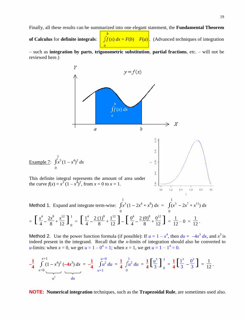
Finally, all these results can be summarized into one elegant statement, the Fundamental Theorem

of Calculus for definite integrals:

a

b

f (x) dx = F(b) F(a) . (Advanced techniques of integration

– such as integration by parts, trigonometric substitution, partial fractions, etc. – will not be

reviewed here.)

Example 7: 0

1

x3 (1 x

4)2 dx

This definite integral represents the amount of area under

the curve f(x) = x3 (1 – x

4)2, from x = 0 to x = 1.

Method 1. Expand and integrate term-wise: 0

1

x3 (1 2x

4 + x

8) dx =

0

1

(x3 2x

7 + x

11) dx

= [ x

4

4

2x8

8 +

x12

12 ]

1

0 = [

14

4

2 (1)8

8 +

112

12 ] [

04

4

2 (0)8

8 +

012

12 ] =

1

12 – 0 =

1

12 .

Method 2. Use the power function formula (if possible): If u = 1 – x4, then du = 4x

3 dx, and x

3 is

indeed present in the integrand. Recall that the x-limits of integration should also be converted to

u-limits: when x = 0, we get u = 1 – 04 = 1; when x = 1, we get u = 1 1

4 = 0.

1

4

x=0

x=1

(1 x

4)2 ( 4x

3) dx =

1

4

u=1

u=0

u2 du =

1

4

0

1

u2 du =

1

4 [u

3

3 ]

1

0 =

1

4 [1

3

3

03

3 ] =

1

12 .

NOTE: Numerical integration techniques, such as the Trapezoidal Rule, are sometimes used also.

du u2

20

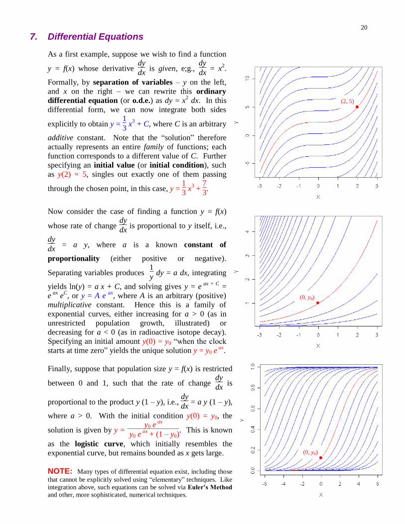
7. Differential Equations

As a first example, suppose we wish to find a function

y = f(x) whose derivative dy

dx is given, e;g.,

dy

dx = x

2.

Formally, by separation of variables – y on the left,

and x on the right – we can rewrite this ordinary

differential equation (or o.d.e.) as dy = x2 dx. In this

differential form, we can now integrate both sides

explicitly to obtain y = 1

3 x

3 + C, where C is an arbitrary

additive constant. Note that the “solution” therefore

actually represents an entire family of functions; each

function corresponds to a different value of C. Further

specifying an initial value (or initial condition), such

as y(2) = 5, singles out exactly one of them passing

through the chosen point, in this case, y = 1

3 x

3 +

7

3.

Now consider the case of finding a function y = f(x)

whose rate of change dy

dx is proportional to y itself, i.e.,

dy

dx = a y, where a is a known constant of

proportionality (either positive or negative).

Separating variables produces 1

y dy = a dx, integrating

yields ln(y) = a x + C, and solving gives y = e ax + C =

e ax e

C, or y = A e

ax, where A is an arbitrary (positive)

multiplicative constant. Hence this is a family of

exponential curves, either increasing for a > 0 (as in

unrestricted population growth, illustrated) or

decreasing for a < 0 (as in radioactive isotope decay).

Specifying an initial amount y(0) = y0 “when the clock

starts at time zero” yields the unique solution y = y0 e ax

.

Finally, suppose that population size y = f(x) is restricted

between 0 and 1, such that the rate of change dy

dx is

proportional to the product y (1 – y), i.e., dy

dx = a y (1 – y),

where a > 0. With the initial condition y(0) = y0, the

solution is given by y = y0 e

ax

y0 e ax

+ (1 – y0). This is known

as the logistic curve, which initially resembles the

exponential curve, but remains bounded as x gets large.

NOTE: Many types of differential equation exist, including those

that cannot be explicitly solved using “elementary” techniques. Like

integration above, such equations can be solved via Euler’s Method

and other, more sophisticated, numerical techniques.

(2, 5)

(0, y0)

(0, y0)

21

8. Summary of Main Points

The instantaneous rate of change of a function y = f(x) at a value of x in its domain, is given by its

derivative dy

dx = f

(x). This function is mathematically defined in terms of a particular “limiting value”

of average rates of change over progressively smaller intervals (when that limit exists), and can be

interpreted as the slope of the line tangent to the graph of y = f(x). As complex functions are built up

from simpler ones by taking sums, differences, products, quotients, and compositions, formulas exist

for computing their derivatives as well. In particular, via the Chain Rule d

dx [f(u)] = f (u)

du

dx , we

have: d

dx (u

p) = p u

p 1 du

dx General Power Rule

d

dx (e

u) = e

u du

dx General Exponential Rule

d

dx [ln(u)] =

1

u du

dx General Logarithm Rule

Derivatives can be applied to estimate functions locally, find the relative extrema of functions, and

relate rates of change of different but connected functions.

A function f(x) has an antiderivative F(x) if its derivative dF

dx = f(x), or equivalently, f(x) dx = dF, and

expressed in terms of an indefinite integral: f (x) dx = F(x) + C. In particular:

u p du =

u p+1

p + 1 + C, if p 1 General Power Rule

u1 du = ln |u| + C General Logarithm Rule

e u du = e

u + C General Exponential Rule

The corresponding definite integral

a

b

f(x) dx = F(b) F(a) is commonly interpreted as the area

under the graph of y = f(x) in the interval [a, b], though other interpretations do exist. Other

quantities that can be interpreted as definite integrals include volume, surface area, arc length,

amount of work done over a path, average value, probability, and many others.

Derivatives and integrals can be generally be used to analyze the dynamical behavior of complex

systems, for example, via differential equations of various types. Numerical methods are often

used when explicit solutions are intractable.

Suggestions for improving this document? Send them to ifischer@wisc.edu.