nonparametric test - pages.stat.wisc.edupages.stat.wisc.edu/~st571-1/fall2005/lec18-21.2.pdf ·...

Nonparametric Methods for Two Samples

An overview

• In the independent two-sample t-test, we assume normality,independence, and equal variances.

• This t-test is robust against nonnormality, but is sensitiveto dependence.

• If n1 is close to n2, then the test is moderately robust againstunequal variance (σ2

1 6= σ22). But if n1 and n2 are quite

different (e.g. differ by a ratio of 3 or more), then the testis much less robust.

• How to determine whether the equal variance assumption isappropriate?

• Under normality, we can compare σ21 and σ2

2 using S21 and

S22 , but such tests are very sensitive to nonnormality. Thus

we avoid using them.

• Instead we consider a nonparametric test called Levene’stest for comparing two variances, which does not assumenormality while still assuming independence.

• Later on we will also consider nonparametric tests for com-paring two means.

193


Levene’s test

Consider two independent samples Y1 and Y2:

Sample 1: 4, 8, 10, 23

Sample 2: 1, 2, 4, 4, 7

Test H0 : σ21 = σ2

2 vs HA : σ21 6= σ2

2.

• Note that s21 = 67.58, s2

2 = 5.30.

• The main idea of Levene’s test is to turn testing for equalvariances using the original data into testing for equal meansusing modified data.

• Suppose normality and independence, if Levene’s test givesa small p-value (< 0.01), then we use an approximate testfor H0 : µ1 = µ2 vs HA : µ1 6= µ2. See Section 10.3.2 of thebluebook.

194


Levene’s test

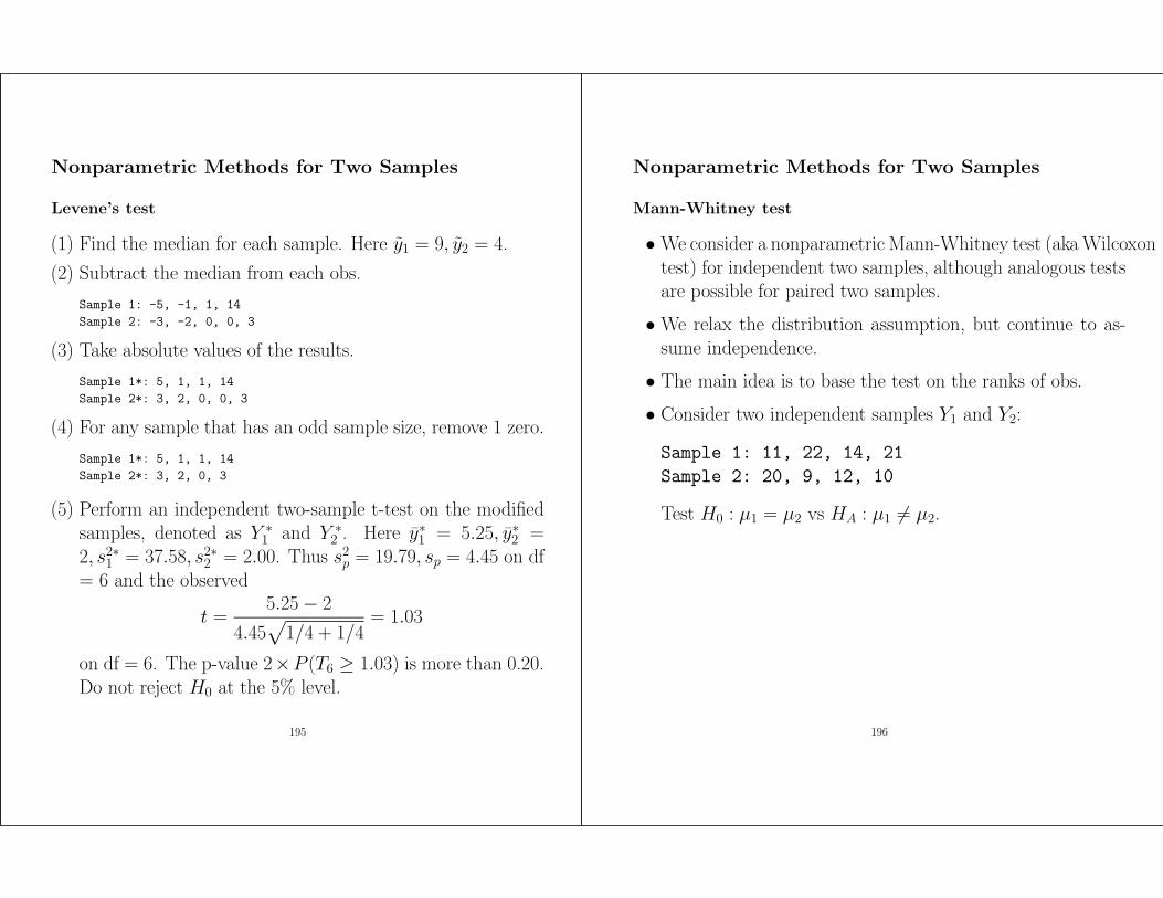
(1) Find the median for each sample. Here y1 = 9, y2 = 4.

(2) Subtract the median from each obs.

Sample 1: -5, -1, 1, 14

Sample 2: -3, -2, 0, 0, 3

(3) Take absolute values of the results.

Sample 1*: 5, 1, 1, 14

Sample 2*: 3, 2, 0, 0, 3

(4) For any sample that has an odd sample size, remove 1 zero.

Sample 1*: 5, 1, 1, 14

Sample 2*: 3, 2, 0, 3

(5) Perform an independent two-sample t-test on the modifiedsamples, denoted as Y ∗

1 and Y ∗2 . Here y∗1 = 5.25, y∗2 =

2, s2∗1 = 37.58, s2∗

2 = 2.00. Thus s2p = 19.79, sp = 4.45 on df

= 6 and the observed

t =5.25 − 2

4.45√

1/4 + 1/4= 1.03

on df = 6. The p-value 2×P (T6 ≥ 1.03) is more than 0.20.Do not reject H0 at the 5% level.

195


Mann-Whitney test

• We consider a nonparametric Mann-Whitney test (aka Wilcoxontest) for independent two samples, although analogous testsare possible for paired two samples.

• We relax the distribution assumption, but continue to as-sume independence.

• The main idea is to base the test on the ranks of obs.

• Consider two independent samples Y1 and Y2:

Sample 1: 11, 22, 14, 21

Sample 2: 20, 9, 12, 10

Test H0 : µ1 = µ2 vs HA : µ1 6= µ2.

196


Mann-Whitney test

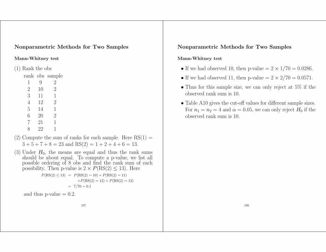
(1) Rank the obs

rank obs sample1 9 22 10 23 11 14 12 25 14 16 20 27 21 18 22 1

(2) Compute the sum of ranks for each sample. Here RS(1) =3 + 5 + 7 + 8 = 23 and RS(2) = 1 + 2 + 4 + 6 = 13.

(3) Under H0, the means are equal and thus the rank sumsshould be about equal. To compute a p-value, we list allpossible ordering of 8 obs and find the rank sum of eachpossibility. Then p-value is 2 × P (RS(2) ≤ 13). Here

P (RS(2) ≤ 13) = P (RS(2) = 10) + P (RS(2) = 11)

+P (RS(2) = 12) + P (RS(2) = 13)

= 7/70 = 0.1

and thus p-value = 0.2.

197


Mann-Whitney test

• If we had observed 10, then p-value = 2 × 1/70 = 0.0286.

• If we had observed 11, then p-value = 2 × 2/70 = 0.0571.

• Thus for this sample size, we can only reject at 5% if theobserved rank sum is 10.

• Table A10 gives the cut-off values for different sample sizes.For n1 = n2 = 4 and α = 0.05, we can only reject H0 if theobserved rank sum is 10.

198


Mann-Whitney test

Recorded below are the longevity of two breeds of dogs.Breed A Breed Bobs rank obs rank12.4 9 11.6 715.9 14 9.7 411.7 8 8.8 314.3 11.5 14.3 11.510.6 6 9.8 58.1 2 7.7 113.2 1016.6 1519.3 1615.1 13n2 = 10 n1 = 6

T ∗ = 31.5

199


Mann-Whitney test

• Here n1 is the sample size in the smaller group and n2 is thesample size in the larger group.

• T ∗ is the sum of ranks in the smaller group. Let T ∗∗ =n1(n1 + n2 + 1) − T ∗ = 6 × 17 − 31.5 = 70.5.

• Let T = min(T ∗, T ∗∗) = 31.5 and look up Table A10.

• Since the observed T is between 27 and 32, the p-value isbetween 0.01 and 0.05. Reject H0 at 5%.

Remarks

• If there are ties, Table A10 gives approximation only.

• The test does not work well if the variances are very differ-ent.

• It is not easy to extend the idea to more complex types ofdata. There is no CI.

• For paired two samples, consider using signed rank test.

• See p.251 of the bluebook for a decision tree.

200


Key R commands

> # Levene’s test

> levene.test = function(data1, data2){

+ levene.trans = function(data){

+ a = sort(abs(data-median(data)))

+ if (length(a)%%2)

+ a[a!=0|duplicated(a)]

+ else a

+ }

+ t.test(levene.trans(data1), levene.trans(data2), var.equal=T)

+ }

> y1 = c(4,8,10,23)

> y2 = c(1,2,4,4,7)

> levene.test(y1, y2)

Two Sample t-test

data: levene.trans(data1) and levene.trans(data2)

t = 1.0331, df = 6, p-value = 0.3414

alternative hypothesis: true difference in means is not equal to 0

95 percent confidence interval:

-4.447408 10.947408

sample estimates:

mean of x mean of y

5.25 2.00

>

> # Mann-Whitney test example

> samp1 = c(11, 22, 14, 21)

> samp2 = c(20, 9, 12, 10)

> # W = 23-10 = 13

> wilcox.test(samp1, samp2)

Wilcoxon rank sum test

data: samp1 and samp2

W = 13, p-value = 0.2

alternative hypothesis: true mu is not equal to 0

201

>

> breedA = c(12.4, 15.9, 11.7, 14.3, 10.6, 8.1, 13.2, 16.6, 19.3, 15.1)

> breedB = c(11.6, 9.7, 8.8, 14.3, 9.8, 7.7)

> # W = 70.5-21 = 49.5

> wilcox.test(breedA, breedB)

Wilcoxon rank sum test with continuity correction

data: breedA and breedB

W = 49.5, p-value = 0.03917

alternative hypothesis: true mu is not equal to 0

Warning message:

Cannot compute exact p-value with ties in: wilcox.test.default(breedA, breedB)

>

202

Comparing Two Proportions

Test procedure

Consider two binomial distributions Y1 ∼ B(n1, p1), Y2 ∼ B(n2, p2),and Y1, Y2 are independent. We want to test

H0 : p1 = p2 vs HA : p1 6= p2

• Use the point estimator p1 − p2, where p1 = Y1/n1, p2 =Y2/n2 are the sample proportions.

• Note that µp1−p2 = E(p1 − p2) = p1 − p2 and σ2p1−p2

=V ar(p1 − p2) = p1(1 − p1)/n1 + p2(1 − p2)/n2.

• Under H0 : p1 = p2 = p, µp1−p2 = 0 and σ2p1−p2

= p(1 −p)(1/n1 + 1/n2).

• Under H0, the test statistic is approximately normal,

Z =p1 − p2 − 0

√

p(1 − p)(1/n1 + 1/n2)≈ N(0, 1)

• But we do not know p and thus estimate it by

p =Y1 + Y2

n1 + n2

• Thus the test statistic is Z = p1−p2−0√p(1−p)(1/n1+1/n2)

≈ N(0, 1)

under H0.

203


Potato cure rate example

A plant pathologist is interested in comparing the effectivenessof two fungicide used on infested potato plants. Let Y1 denotethe number of plants cured using fungicide A among n1 plantsand let Y2 denote the number of plants cured using fungicideB among n2 plants. Assume that Y1 ∼ B(n1, p1) and Y2 ∼B(n2, p2), where p1 is the cure rate of fungicide A and p2 is thecure rate of fungicide B. Suppose the obs are n1 = 105, p1 = 71for fungicide A and n2 = 87, p2 = 45 for fungicide B. TestH0 : p1 = p2 vs HA : p1 6= p2.

• Here p1 = 71/105 = 0.676, p2 = 45/87 = 0.517, and thepooled estimate of cure rate is

p =71 + 45

105 + 87= 0.604

• Thus the observed test statistic is

z =(0.676 − 0.517) − 0

√

0.604 × 0.396 × (1/105 + 1/87)= 2.24

• Compared to Z, the p-value is 2 × P (Z ≥ 2.24) = 0.025.

• Reject H0 at the 5% level. There is moderate evidenceagainst H0.

204


Remarks

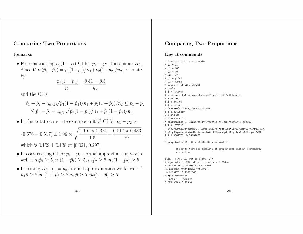
• For constructing a (1 − α) CI for p1 − p2, there is no H0.Since V ar(p1−p2) = p1(1−p1)/n1+p2(1−p2)/n2, estimateby

p1(1 − p1)

n1+

p2(1 − p2)

n2

and the CI is

p1 − p2 − zα/2

√

p1(1 − p1)/n1 + p2(1 − p2)/n2 ≤ p1 − p2

≤ p1 − p2 + zα/2

√

p1(1 − p1)/n1 + p2(1 − p2)/n2

• In the potato cure rate example, a 95% CI for p1 − p2 is

(0.676 − 0.517) ± 1.96 ×√

0.676 × 0.324

105+

0.517 × 0.483

87

which is 0.159 ± 0.138 or [0.021, 0.297].

• In constructing CI for p1− p2, normal approximation workswell if n1p1 ≥ 5, n1(1 − p1) ≥ 5, n2p2 ≥ 5, n2(1 − p2) ≥ 5.

• In testing H0 : p1 = p2, normal approximation works well ifn1p ≥ 5, n1(1 − p) ≥ 5, n2p ≥ 5, n2(1 − p) ≥ 5.

205


Key R commands

> # potato cure rate example

> y1 = 71

> n1 = 105

> y2 = 45

> n2 = 87

> p1 = y1/n1

> p2 = y2/n2

> poolp = (y1+y2)/(n1+n2)

> poolp

[1] 0.6041667

> z.value = (p1-p2)/sqrt(poolp*(1-poolp)*(1/n1+1/n2))

> z.value

[1] 2.241956

> # p-value

> 2*pnorm(z.value, lower.tail=F)

[1] 0.02496419

> # 95% CI

> alpha = 0.05

> qnorm(alpha/2, lower.tail=F)*sqrt(p1*(1-p1)/n1+p2*(1-p2)/n2)

[1] 0.1379716

> c(p1-p2-qnorm(alpha/2, lower.tail=F)*sqrt(p1*(1-p1)/n1+p2*(1-p2)/n2),

+ p1-p2+qnorm(alpha/2, lower.tail=F)*sqrt(p1*(1-p1)/n1+p2*(1-p2)/n2))

[1] 0.02097751 0.29692068

>

> prop.test(c(71, 45), c(105, 87), correct=F)

2-sample test for equality of proportions without continuity

correction

data: c(71, 45) out of c(105, 87)

X-squared = 5.0264, df = 1, p-value = 0.02496

alternative hypothesis: two.sided


0.02097751 0.29692068

sample estimates:

prop 1 prop 2

0.6761905 0.5172414

206

>

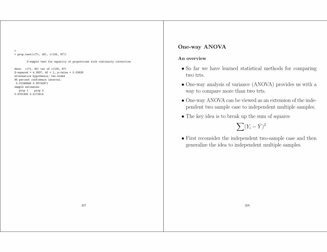
> prop.test(c(71, 45), c(105, 87))

2-sample test for equality of proportions with continuity correction

data: c(71, 45) out of c(105, 87)

X-squared = 4.3837, df = 1, p-value = 0.03628

alternative hypothesis: two.sided


0.01046848 0.30742971

sample estimates:

prop 1 prop 2

0.6761905 0.5172414

207

One-way ANOVA

An overview

• So far we have learned statistical methods for comparingtwo trts.

• One-way analysis of variance (ANOVA) provides us with away to compare more than two trts.

• One-way ANOVA can be viewed as an extension of the inde-pendent two sample case to independent multiple samples.

• The key idea is to break up the sum of squares∑

(Yi − Y )2

• First reconsider the independent two-sample case and thengeneralize the idea to independent multiple samples.

208

One-way ANOVA

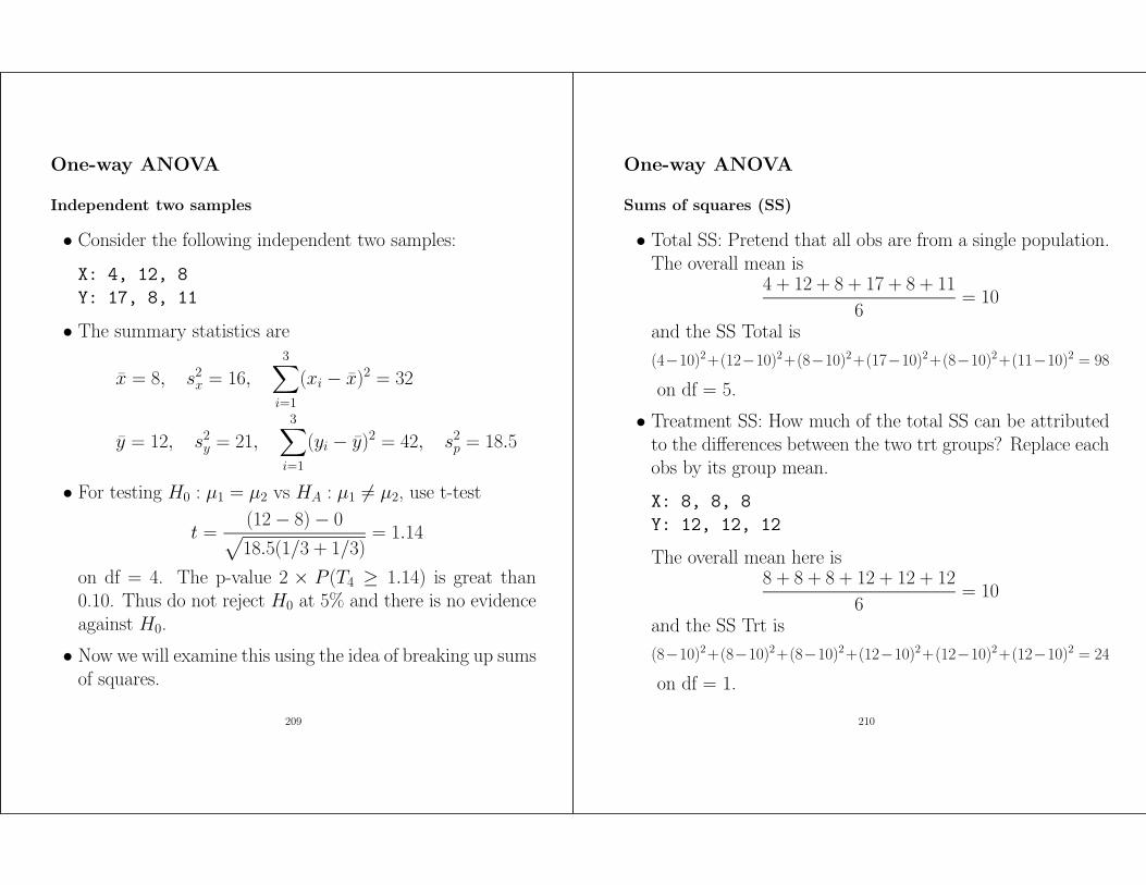
Independent two samples

• Consider the following independent two samples:

X: 4, 12, 8

Y: 17, 8, 11

• The summary statistics are

x = 8, s2x = 16,

3∑

i=1

(xi − x)2 = 32

y = 12, s2y = 21,

3∑

i=1

(yi − y)2 = 42, s2p = 18.5

• For testing H0 : µ1 = µ2 vs HA : µ1 6= µ2, use t-test

t =(12 − 8) − 0

√

18.5(1/3 + 1/3)= 1.14

on df = 4. The p-value 2 × P (T4 ≥ 1.14) is great than0.10. Thus do not reject H0 at 5% and there is no evidenceagainst H0.

• Now we will examine this using the idea of breaking up sumsof squares.

209

One-way ANOVA

Sums of squares (SS)

• Total SS: Pretend that all obs are from a single population.The overall mean is

4 + 12 + 8 + 17 + 8 + 11

6= 10

and the SS Total is

(4−10)2+(12−10)2+(8−10)2+(17−10)2+(8−10)2+(11−10)2 = 98

on df = 5.

• Treatment SS: How much of the total SS can be attributedto the differences between the two trt groups? Replace eachobs by its group mean.

X: 8, 8, 8

Y: 12, 12, 12

The overall mean here is8 + 8 + 8 + 12 + 12 + 12

6= 10

and the SS Trt is

(8−10)2+(8−10)2+(8−10)2+(12−10)2+(12−10)2+(12−10)2 = 24

on df = 1.

210

One-way ANOVA

Sums of squares (SS)

• Error SS: How much of the total SS can be attributed tothe differences within each trt group? The SS Error is

(4− 8)2 +(12− 8)2 +(8− 8)2 +(17− 12)2 +(8− 12)2 +(11− 12)2 = 74

on df = 4.

• Note that SSError/df = 74/4 = 18.5 = s2p.

• Note also that

SS Total = SS Trt + SS Error (98 = 24 + 74)df Total = df Trt + df Error (5 = 1 + 4)

• An ANOVA table summarizes the information.

Source df SS MSTrt 1 24 24Error 4 74 18.5Total 5 98 –

• Here MS = SS/df.

211

One-way ANOVA

F-test

• H0 : µ1 = µ2 vs HA : µ1 6= µ2

• A useful fact is that, under H0, the test statistic is:

F =MSTrt

MSError∼ FdfTrt,dfError

• In the example, the observed f = 24/18.5 = 1.30.

• Compare this to an F-distribution with 1 df in the numeratorand 4 df in the denominator using Table D. The (one-sided)p-value P (F1,4 ≥ 1.30) is greater than 0.10. Do not rejectH0 at the 10% level. There is no evidence against H0.

• Note that a small difference between the two trt means rel-ative to variability is associated with a small f , a large p-value, and accepting H0, whereas a large difference betweenthe two trt means relative to variability is associated with alarge f , a small p-value, and rejecting H0.

• Note that f = 1.30 = (1.14)2 = t2. That is f = t2, butonly when the df in the numerator is 1.

• Note that the p-value is one-tailed, even though HA is two-sided.

212

One-way ANOVA

A recap

In the simple example above, there are 2 trts and 3 obs/trt.The overall mean is 10,

SSTotal =3

∑

i=1

(xi − 10)2 +3

∑

i=1

(yi − 10)2 = 98

SSTrt = 3 × (x − 10)2 + 3 × (y − 10)2 = 24

SSError =3

∑

i=1

(xi − 8)2 +3

∑

i=1

(yi − 12)2 = 74

with df = 5, 1, and 4, respectively.

213

One-way ANOVA

Generalization to k independent samples

• Consider k trts and ni obs for the ith trt.

• Let yij denote the jth obs in the ith trt group.

• Tabulate the obs as follows.

Trt 1 2 · · · kObs y11 y21 · · · yk1

y12 y22 · · · yk2... ... ...

y1n1 y2n2 · · · yknk

Sum y1· y2· · · · yk· y··Mean y1· y2· · · · yk· y··

Trt 1 2 310 9 67 12 28 6 412 7

9Sum 37 27 28 92Mean 9.25 9 5.6 7.67

• Sum for the ith trt: yi· =∑ni

j=1 yij

• Mean for the ith trt: yi· = yi·/ni

• Grand sum: y·· =∑k

i=1

∑nij=1 yij =

∑ki=1 yi·

• Grand mean: y·· = y··/N where the total # of obs is:

N =k

∑

i=1

ni = n1 + n2 + · · · + nk.

214

One-way ANOVA

Basic partition of SS

SS Total = SS Trt + SS Errordf Total = df Trt + df Error

where

SS Total =k

∑

i=1

ni∑

j=1

(yij − y··)2 =

k∑

i=1

ni∑

j=1

y2ij −

y2··

N

df Total = N − 1

SS Trt =k

∑

i=1

ni(yi· − y··)2 =

k∑

i=1

y2i·

ni− y2

··N

=

df Trt = k − 1

SS Error =k

∑

i=1

ni∑

j=1

(yij − yi·)2

= (n1 − 1)s21 + (n2 − 1)s2

2 + · · · + (nk − 1)s2k

df Error = N − k = (n1 − 1) + · · · + (nk − 1)

or simply SS Error = SS Total - SS Trt anddf Error = df Total - df Trt.

215

One-way ANOVA

Fish length example

• Consider the length of fish (in inch) that are subject to oneof three types of diet, with seven observations per diet group.The raw data are:

Y1 18.2 20.1 17.6 16.8 18.8 19.7 19.1Y2 17.4 18.7 19.1 16.4 15.9 18.4 17.7Y3 15.2 18.8 17.7 16.5 15.9 17.1 16.7

• A stem and leaf display of these data looks like:

Y1 Y2 Y3

15. 9 2916. 8 4 5717. 6 47 7118. 28 74 819. 71 120. 1

• Summary statistics are:

y1· = 130.3 y1· = 18.61 s21 = 1.358 n1 = 7

y2· = 123.6 y2· = 17.66 s22 = 1.410 n2 = 7

y3· = 117.9 y3· = 16.84 s23 = 1.393 n3 = 7

y·· = 371.8 y·· = 17.70 N = 21

216

One-way ANOVA

Fish length example

• The sums of squares are:

SSTotal =3

∑

i=1

7∑

j=1

y2ij −

(y··)2

N

= 6618.60 − 6582.63 = 35.97

SSTrt =3

∑

i=1

(yi·)2

ni− (y··)

2

N

=1

7[(130.3)2 + (123.6)2 + (117.9)2] − 6582.63

= 11.01

SSErr = SSTot − SSTrt = 35.97 − 11.01 = 24.96

• Or SSErr = 6s21 + 6s2

2 + 6s23 = 24.96

• The corresponding ANOVA table is:

Source df SS MSTrt 2 11.01 5.505Error 18 24.96 1.387Total 20 35.97

217

One-way ANOVA

Fish length example

• Note that the MS for Error computed above is the same asthe pooled estimate of variance, s2

p.

• The null hypothesis H0: “all population means are equal”versus the alternative hypothesis HA: “not all populationmeans are equal”.

• The observed test statistic is:

f =MSTrt

MSErr=

5.505

1.387= 3.97

• Compare this with F2,18 from Table D: at 5% f2,18 = 3.55,and at 1% f2,18 = 6.01, so for our data 0.01 < p-value <0.05.

• Reject H0 at the 5% level. There is moderate evidenceagainst H0. That is, there is moderate evidence that thereis a diet effect on the fish length.

218

One-way ANOVA

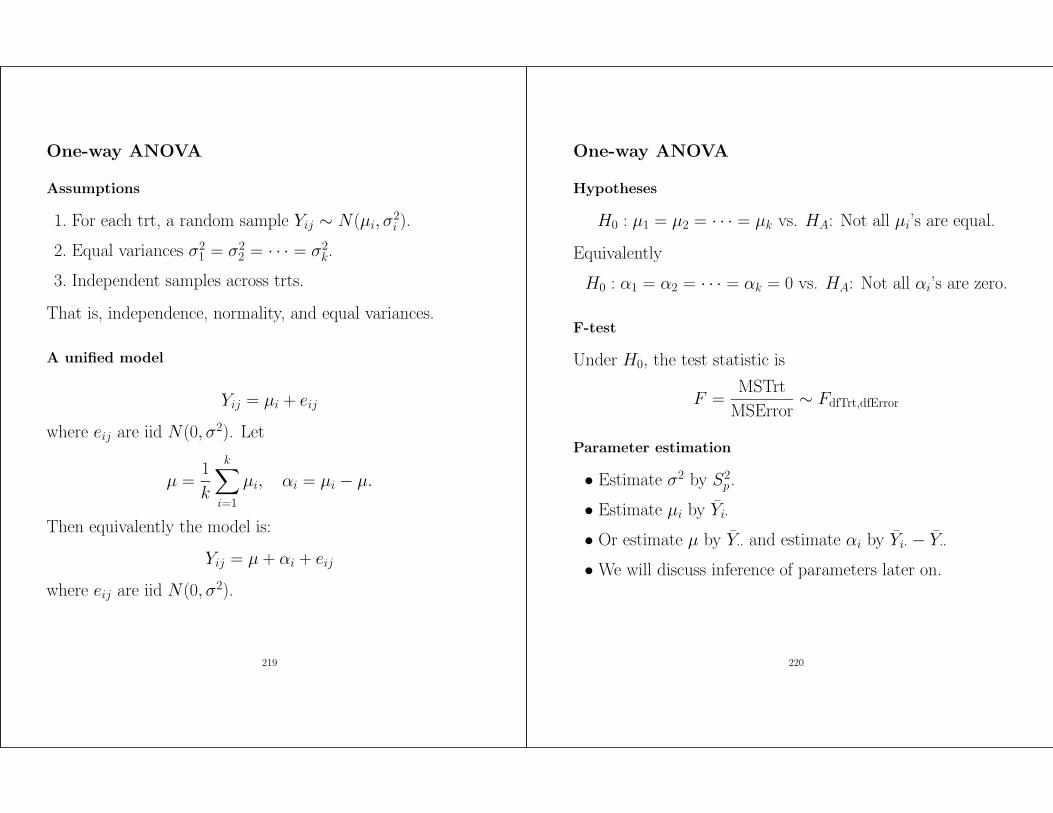
Assumptions

1. For each trt, a random sample Yij ∼ N(µi, σ2i ).

2. Equal variances σ21 = σ2

2 = · · · = σ2k.

3. Independent samples across trts.

That is, independence, normality, and equal variances.

A unified model

Yij = µi + eij

where eij are iid N(0, σ2). Let

µ =1

k

k∑

i=1

µi, αi = µi − µ.

Then equivalently the model is:

Yij = µ + αi + eij

where eij are iid N(0, σ2).

219

One-way ANOVA

Hypotheses

H0 : µ1 = µ2 = · · · = µk vs. HA: Not all µi’s are equal.

Equivalently

H0 : α1 = α2 = · · · = αk = 0 vs. HA: Not all αi’s are zero.

F-test

Under H0, the test statistic is

F =MSTrt

MSError∼ FdfTrt,dfError

Parameter estimation

• Estimate σ2 by S2p .

• Estimate µi by Yi·

• Or estimate µ by Y·· and estimate αi by Yi· − Y··

• We will discuss inference of parameters later on.

220

One-way ANOVA

A brief review

Dist’n One-Sample Inference Two-Sample Inference

Normal H0 : µ = µ0 Paired H0 : µD = 0, CI for µD (Z or Tn−1)

CI for µ 2 ind samples H0 : µ1 = µ2, CI for µ1 − µ2 (Tn1+n2−2)

σ2 is known (Z) or unknown (Tn−1) k ind samples H0 : µ1 = µ2 = · · · = µk (Fk−1,N−k)

H0 : σ2 = σ20, CI for σ2 (χ2

n−1) H0 : σ2 = σ20, CI for σ2 (χ2

N−k)

Arbitrary H0 : µ = µ0, CI for µ (CLT Z) Paired H0 : µD = 0 (Signed rank)

2 ind samples H0 : µ1 = µ2 (Mann-Whitney)

2 ind samples H0 : σ21 = σ2

2 (Levene’s)

Binomial H0 : p = p0 (Binomial Y ∼ B(n, p))H0 : p = p0, CI for p (CLT Z) 2 ind samples H0 : p1 = p2, CI for p1 − p2 (CLT Z)

• For testing or CI, address model assumptions (e.g. normal-ity, independence, equal variance) via detection, correction,and robustness.

• In hypothesis testing, H0, HA (1-sided or 2-sided), teststatistic and its distribution, p-value, interpretation, rejec-tion region, α, β, power, sample size determination.

• For paired t-test, the assumptions are D ∼ iid N(µD, σ2D)

where D = Y1 − Y2. Y1, Y2 need not be normal. Y1 and Y2

need not be independent.

221

One-way ANOVA

More on assumptions

Assumptions DetectionNormality Stem-and-leaf plot; normal scores plot

Independence Study designEqual variance Levene’s testCorrect model More later

Detect unequal variance

• Plot trt standard deviation vs trt mean.

• Or use an extension of Levene’s test for

H0 : σ21 = σ2

2 = · · · = σ2k.

The main idea remains the same, except that a one-wayANOVA is used instead of a two-sample t-test.

222

One-way ANOVA

Levene’s test

For example, consider k = 3 groups of data.

Sample 1: 2, 5, 7, 10

Sample 2: 4, 8, 19

Sample 3: 1, 2, 4, 4, 7

(1) Find the median for each sample. Here y1 = 6, y2 = 8, y3 =4.

(2) Subtract the median from each obs and take absolute values.

Sample 1*: 4, 1, 1, 4

Sample 2*: 4, 0, 11

Sample 3*: 3, 2, 0, 0, 3

(3) For any sample that has an odd sample size, remove 1 zero.

Sample 1*: 4, 1, 1, 4

Sample 2*: 4, 11

Sample 3*: 3, 2, 0, 3

(4) Perform a one-way ANOVA f-test on the final results.

Source df SS MS F p-valueGroup 2 44.6 22.30 3.95 0.05 < p < 0.10Error 7 39.5 5.64 –Total 9 84.1 – –

223

One-way ANOVA

Key R commands

> # Fish length example

> y1 = c(18.2,20.1,17.6,16.8,18.8,19.7,19.1)

> y2 = c(17.4,18.7,19.1,16.4,15.9,18.4,17.7)

> y3 = c(15.2,18.8,17.7,16.5,15.9,17.1,16.7)

> y = c(y1, y2, y3)

> n1 = length(y1)

> n2 = length(y2)

> n3 = length(y3)

> trt = c(rep(1,n1),rep(2,n2),rep(3,n3))

> oneway.test(y~factor(trt), var.equal=T)

One-way analysis of means

data: y and factor(trt)

F = 3.9683, num df = 2, denom df = 18, p-value = 0.03735

> fit.lm = lm(y~factor(trt))

> anova(fit.lm)

Analysis of Variance Table

Response: y

Df Sum Sq Mean Sq F value Pr(>F)

factor(trt) 2 11.0067 5.5033 3.9683 0.03735 *

Residuals 18 24.9629 1.3868

---

Signif. codes: 0 ‘***’ 0.001 ‘**’ 0.01 ‘*’ 0.05 ‘.’ 0.1 ‘ ’ 1

>

> # Alternatively use data frame

> eg = data.frame(y=y, trt=factor(trt))

> eg

y trt

1 18.2 1

2 20.1 1

3 17.6 1

4 16.8 1

5 18.8 1

6 19.7 1

224

7 19.1 1

8 17.4 2

9 18.7 2

10 19.1 2

11 16.4 2

12 15.9 2

13 18.4 2

14 17.7 2

15 15.2 3

16 18.8 3

17 17.7 3

18 16.5 3

19 15.9 3

20 17.1 3

21 16.7 3

> eg.lm = lm(y~trt, eg)

> anova(eg.lm)

Analysis of Variance Table

Response: y

Df Sum Sq Mean Sq F value Pr(>F)

trt 2 11.0067 5.5033 3.9683 0.03735 *

Residuals 18 24.9629 1.3868

---

Signif. codes: 0 ‘***’ 0.001 ‘**’ 0.01 ‘*’ 0.05 ‘.’ 0.1 ‘ ’ 1

>

> # Kruskal-Wallis rank sum test

> kruskal.test(y~trt)

Kruskal-Wallis rank sum test

data: y by trt

Kruskal-Wallis chi-squared = 5.7645, df = 2, p-value = 0.05601

225

Comparisons among Means

An overview

• In one-way ANOVA, if we reject H0, then we know that notall trt means are the same.

• But this may not be informative enough. We now considerparticular comparisons of trt means.

• We will consider contrasts and all pairwise comparisons.

226


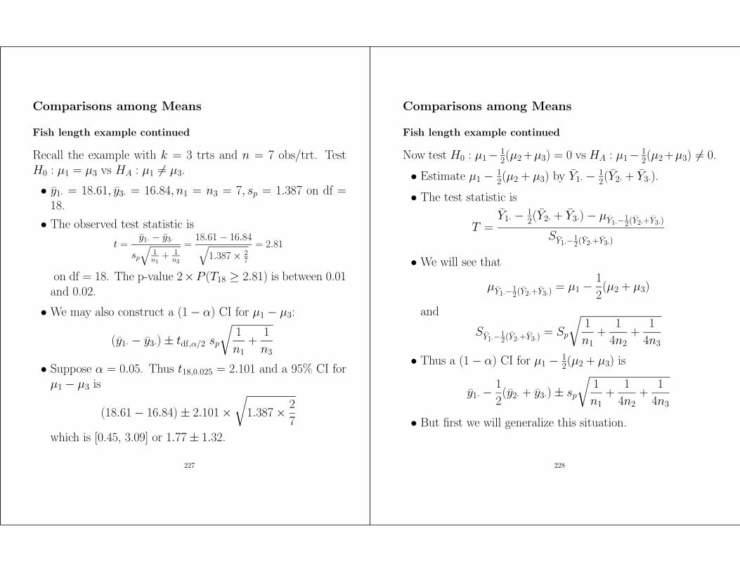
Fish length example continued

Recall the example with k = 3 trts and n = 7 obs/trt. TestH0 : µ1 = µ3 vs HA : µ1 6= µ3.

• y1· = 18.61, y3· = 16.84, n1 = n3 = 7, sp = 1.387 on df =18.

• The observed test statistic is

t =y1· − y3·

sp

√

1n1

+ 1n3

=18.61 − 16.84√

1.387 × 27

= 2.81

on df = 18. The p-value 2×P (T18 ≥ 2.81) is between 0.01and 0.02.

• We may also construct a (1 − α) CI for µ1 − µ3:

(y1· − y3·) ± tdf,α/2 sp

√

1

n1+

1

n3

• Suppose α = 0.05. Thus t18,0.025 = 2.101 and a 95% CI forµ1 − µ3 is

(18.61 − 16.84) ± 2.101 ×√

1.387 × 2

7

which is [0.45, 3.09] or 1.77 ± 1.32.

227



Now test H0 : µ1− 12(µ2 +µ3) = 0 vs HA : µ1− 1

2(µ2 +µ3) 6= 0.

• Estimate µ1 − 12(µ2 + µ3) by Y1· − 1

2(Y2· + Y3·).

• The test statistic is

T =Y1· − 1

2(Y2· + Y3·) − µY1·−12(Y2·+Y3·)

SY1·−12(Y2·+Y3·)

• We will see that

µY1·−12(Y2·+Y3·)

= µ1 −1

2(µ2 + µ3)

and

SY1·−12(Y2·+Y3·)

= Sp

√

1

n1+

1

4n2+

1

4n3

• Thus a (1 − α) CI for µ1 − 12(µ2 + µ3) is

y1· −1

2(y2· + y3·) ± sp

√

1

n1+

1

4n2+

1

4n3

• But first we will generalize this situation.

228


Contrast

• A contrast is a quantity of the form

k∑

i=1

λiµi

where k is the # of trts, µi is the ith trt mean, and λi is theith contrast coefficient.

• For comparison, we require that∑k

i=1 λi = 0.

• For example, we have seen two contrasts already.

• µ1 − µ3 is a contrast with λ1 = 1, λ2 = 0, λ3 = −1:

k∑

i=1

λiµi = 1 × µ1 + 0 × µ2 + (−1) × µ3.

• µ1 − 12(µ2 + µ3) is a contrast with λ1 = 1, λ2 = −1/2, λ3 =

−1/2:

k∑

i=1

λiµi = 1 × µ1 + (−1/2) × µ2 + (−1/2) × µ3.

229


Contrast

• Estimate∑k

i=1 λiµi by X =∑k

i=1 λiYi·

• Consider the distribution of

T =X − µX

SX

• Here µX =∑k

i=1 λiµi, because

µX = E(k

∑

i=1

λiYi·) =k

∑

i=1

λiE(Yi·) =k

∑

i=1

λiµi.

• For SX , consider variance first.

V ar(k

∑

i=1

λiYi·) =k

∑

i=1

λ2iV ar(Yi·) =

k∑

i=1

λ2i

σ2

ni= σ2

k∑

i=1

λ2i

ni.

• Estimate V ar(∑k

i=1 λiYi·) by S2p

∑ki=1

λ2i

niand

SX = Sp

√

√

√

√

k∑

i=1

λ2i

ni

230



• For the first contrast, λ1 = 1, λ2 = 0, λ3 = −1,

SX = Sp

√

1

7+

0

7+

1

7= Sp

√

2

7

as before.

• For the second contrast, λ1 = 1, λ2 = −1/2, λ3 = −1/2,

SX = Sp

√

1

7+

1/4

7+

1/4

7= Sp

√

3

14

• Thus for testing H0 : µ1− 12(µ2 +µ3) = 0, the observed test

statistic is

t =y1· − 1

2(y2· + y3·)

sp

√

314

=18.61 − (17.66 + 16.84)/2

√

1.387 × 314

= 2.49

on df = 18. The p-value 2× P (T18 ≥ 2.49) is between 0.02and 0.05.

231



• We may also construct a 95% CI for µ1 − 12(µ2 + µ3):

y1· −1

2(y2· + y3·) ± t18,0.025 sp

√

3

14

• A 95% CI for µ1 − 12(µ2 + µ3) is

18.61 − 1

2(17.66 + 16.84) ± 2.101 ×

√

1.387 × 3

14

which is [0.21, 2.51] or 1.36 ± 1.15.

232


Remarks

• If all ni = n, then

V ar(k

∑

i=1

λiYi·) =σ2

n

k∑

i=1

λ2i .

This is called a balanced case.

• Single sample SY = S√

1n

• Two samples SY1−Y2= Sp

√

1n1

+ 1n2

• Multiple samples

S∑ki=1 λiYi·

= Sp

√

√

√

√

k∑

i=1

λ2i

ni

233

nonparametric test - pages.stat.wisc.edupages.stat.wisc.edu/~st571-1/fall2005/lec18-21.2.pdf ·...

Documents