backscattering from a dielectric surface with a …
TRANSCRIPT

1. 10 0.1 1 10.
frequency (1/m)
rough
large scale
100. 1000.
medium scale
-10
0.01
E 0.0001
a~ 0 n
-8 1. 10
Report Series of the Finnish Institute of Marine Research
Merentutkimuslaitos Havsforskningsinstitutet
Finnish Institute of Marine Research
BACKSCATTERING FROM A DIELECTRIC SURFACE WITH A CONTINUOUS ROUGHNESS SPECTRUM
Terhikki Manninen


MERI — Report Series of the Finnish Institute of Marine Research No. 23, 1996
BACKSCATTERING FROM A DIELECTRIC SURFACE WITH A CONTINUOUS ROUGHNESS SPECTRUM
Terhikki Manninen

MERI — Report Series of the Finnish Institute of Marine Research
Cover: Power spectrum of Baltic sea ice
Publisher: Julkaisija:
Finnish Institute of Marine Research
Merentutkimuslaitos P.O. Box 33
PL 33 FIN-00931 Helsinki, Finland
00931 Helsinki
Tel: +3580613941
Puh. 90-613941 Fax: +358061394494
Telekopio: 90-61394 494 e-mail: [email protected] e-mail: [email protected]
Copies of this Report Series may be obtained from the library of the Finnish Institute of Marine Research
Tämän raporttisarjan numeroita voi tilata Merentutkimuslaitoksen kirjastosta.
ISBN 951-53-0800-3 ISSN 1238-5328
0BON444/.?,1
fc:2F /00/ S.;
411 l Recyclable |m° emissions during production
Hakapaino Oy, Helsinki 1996

BACKSCATTERING FROM A DIELECTRIC SURFACE WITH A
CONTINUOUS ROUGHNESS SPECTRUM
CONTENTS
ABSTRACT........ ....... ........ ......... ............................................ .................. .......... 3
1. INTRODUCTION... .............................. ........................ .................. ...... .................. 3
2. SURFACE CORRELATION FOR A CONTINUOUS ROUGHNESS SPECTRUM ................... ............ .......... ........................ ................. 4
3. CALCULATION OF THE BACKSCATTERING COEFFICIENT 8
4, APPLICATION TO BALTIC SEA ICE ......................... ............. 10
5. DISCUSSION ....... ....... ................ ....... ....... ............. ............. .......... ................ 23
6. REFERENCES ..... ........ ...................... ..... ....... .................................... ...... ........ 25


BACKSCATTERING FROM A DIELECTRIC SURFACE WITH A
CONTINUOUS ROUGHNESS SPECTRUM
Terhikki Manninen 1
Finnish Institute of Marine Research
P.O. Box 33, FIFIN-00931 Helsinki, Finland
ABSTRACT
Autocorrelation functions for surfaces with a continuous roughness spectrum have been derived. Explicit equations are given for Gaussian, exponential, isotropic exponential and transformed exponential multiscale surface correlations. These equations are combined with the Integral Equation Method for calculating surface backscattering. The method has been applied to calculating the backscattering coefficient for Baltic sea ice. However, the validity of the approximation of local incidence angles with the radar incidence angle, typically used in IEM calculations, was seriously limited by the small permittivity of ice. As a comparison, average values of the Kirchhoff and complementary field coefficients were calculated using local incidence angles calculated from measured Baltic sea ice surfaces. They turned out to be extremely sensitive to individual large values of local incidence angle and also dependent on the size of the horizontal increment used in the calculation of the local incidence angles. Reliable estimation of the field coefficients requires further investigation.
Key words: multiscale surface roughness, autocorrelation function, backscattering, Baltic Sea, sea ice
1. INTRODUCTION
The recent development of the Integral Equation Method for calculating surface backscattering coefficients has removed the limitation that the surface roughness should be either small or large
compared to the wavelength used (Fung 1994, Fung & Chen 1992, Fung & al. 1992). However, even this method assumes that the surface roughness can be described with the two classical constant parameters, rms height and correlation length. Unfortunately, the rms height and correlation length of natural surfaces like sea ice depend on the measured distance (Church 1988, Keller & al. 1987). Then the use of the IEM equations for calculating the surface backscattering coefficients for such surfaces requires extra consideration. One problem is to find a description for a surface with a continuous roughness spectrum. Another problem is the approximation of the local angle in the field coefficients made in the lEM equations which may not be valid for all surfaces with small dielectric constant values, such as sea ice (Fung 1994).
1Present address: VTT Automation, Space Technology, P.O. Box 13031, FIN-02044 VTT, Finland
4
The problem of surfaces having both small and large scale roughness characteristics has been studied in several cases (Fung 1994, Church 1988, Ulaby & al. 1982, Elson & al. 1980). In an analogous way, a method to take into account a continuous surface roughness spectrum has been developed and is presented in this paper. The problem of field coefficients is presented in the example cases of Baltic sea ice.
2. SURFACE CORRELATION FOR A CONTINUOUS ROUGHNESS SPECTRUM
Natural surfaces are typically results of a sequence of random changes affecting an initial surface. Such surfaces can be treated in the same way as multilayer stacks (Elson & al. 1980). The initial surface is described with a profile z1 (x). A random process h2 (x) then changes the surface profile with an additive roughness so that the new surface profile is z2 (x) = z1 (x) + h2 (x) . The additive roughness can also be negative so that the superposition produces a smoother surface than the original. It is natural to assume that the initial and final surfaces are partially correlated. As more changes take place, more additive components appear and the final surface profile is (Elson & al. 1980)
z„ (x) =z,(x)+ i=2
The final surface correlation function is then obtained as a sum of the original surface correlation and the autocorrelation of the random changes (Elson & al. 1980). Conventional finish analysis uses a sum of exponentials and Gaussians to describe the final surface autocorrelation function (Church 1988)
p() = 62 exp(—M / Li ) 62j exp(—( L1)2 ) (2)
where 6; is the rms height and Li the correlation length of the ith roughness component.
When a surface undergoes changes perpetually due to changing weather conditions (like a sea ice surface), it is natural to replace the summations of Eq. 2 with an integral. Likewise the resulting continuous roughness spectrum is considered to contain a continuous range of spatial frequencies instead of only discrete values.
The estimation of surface correlation parameters is always affected by the inner and outer scales (Elson & Bennet 1979), which give the limits for the minimum and maximum spatial frequencies possible to detect using a certain measurement trace length. Thus, the verification of the continuous roughness spectrum is not trivial. The autocorrelation function and the power spectrum of a surface carry the same information since they are a Fourier transform pair, but the power spectrum is less sensitive to the finite measurement trace length of a profile (Church 1988). However, the surface backscattering coefficient can not be obtained analytically for a general power spectrum. The existing analytical methods for calculating the surface backscattering coefficient for dielectric materials are developed using the autocorrelation function. Therefore an attempt has been made in this paper to develop an autocorrelation function that is not sensitive to the finite length of a profile used to determine the rms height and correlation length values.
In practice, it is impossible to measure all the random changes that have affected the surface. The only possible roughness to be measured is the final result, but one would also need measured values of all the intermediate surfaces to apply Eq. 2 directly. A practical solution is to measure the final surface using various measurement trace lengths from small to large distances so that various final roughness scales are characterized. Since it is not possible to detect the largest roughness components from the smallest distances, it can be thought that the smallest measurement trace lengths give results that would be obtained, if the largest roughness components of Eq. 2 were missing. In addition, the roughness parameters corresponding to a certain distance are dominated by the largest roughness scale that is distinguishable with that measurement trace length. Thus, it is reasonable to think that the roughness
h; (x)
(1)

5
components of the summation in Eq. 2 can be estimated with the roughness components obtained from the final surface using various measurement trace lengths.
For natural surfaces the rms height and the correlation length typically depend on the measured length (Church 1988, Keller & al. 1987). When the dependence is assumed to be of the same form for all roughness components from small to large distances the rms height and correlation length of increasing intervals x; can be described with the following equations
6=f(x), i =1,...,n
A,0 = gft,~; xi ) , i =1,...,n
where f and g denote arbitrary functions. Generalizing the result to a continuously increasing distance with a maximum value xo , we get an equation corresponding to Eq. 2
A,0 =1 f (:)2 0 0
)2 gc~,~;x)dx (5)
xo
where fo = f f (x)2dx so that the value of the correlation function at zero is unity.
If the form of the dependence of rms height and correlation length on distance is not the same in the whole interval of interest, one can divide the interval into sections where the form is invariant and then combine these sections as in the two-scale roughness case.
The behaviour of natural surfaces is often close to that of Brownian surfaces. Then the correlation length L is linearly dependent on the measured length (Church 1988)
L = ko x (6)
where ko is a constant. Also, the logarithm of the iuis height 6 is usually linearly dependent on the logarithm of the measurement trace length x, so that (Keller & al. 1987)
6=c' xb
(7)
where c is a constant.
Commonly used surface correlation functions are Gaussian, exponential, isotropic exponential and transformed exponential given by equations (Fung 1994)
Pft, 0 = exp[—(V +V)/ L2 ]
(8)
= exp[-41 + / L]
(9)
Aft,0 = exp[—V(V +V)/ L2 ]
(10)
Pft,0 = 1 / [1 +(a2 +V) / L213;2
respectively.
(3)
(4)

(z +cz ,iz+b
I 1
+c2 \ --, -b
kö xö ` 2 kö xö )
1+26
I'/ k x~l\ koxo /
-1-2b, 00
1+2b ~ g2 +c2
I'-1-2b, +~2
~ 2 ~
koxo/ \ k°x°
(12)
(13)
(14)
A,C) = 2 (1+2b)
6
The corresponding surface correlation functions corresponding to a continuous roughness spectrum are now according to Eqs. 2-11 (Gradshteyn & Ryzhik 1980, Wolfram 1991)
Pft'C)
_ (1+2b) /~z +C2 \ 3 2 i 3 k 2 x2
2 2 +b kzxz 2F1 2, 2+b;3+b; 2+° 2
( ) o o / \, ~ y ~
(15)
for Gaussian, exponential, isotropic exponential and transformed exponential type of surface correlation respectively. The rms height a, corresponding to the whole surface, is obtained from the rms height 60 , corresponding to the maximum distance x0 , using the following relationship
c = c0 /,/2b+1 (16)
The surface correlation functions corresponding to surfaces of single scale roughness and multiscale roughness are shown in Figure 1 for exponential, transformed exponential and Gaussian cases of equal correlation lengths. The shapes of the multiscale curves require that they be calculated using a longer distance than that of the single scale case to obtain an equally large correlation length (Fig. 2). This is understandable, since the inclusion of smaller roughness scales naturally decreases correlation. Still, the net effect of the inclusion of the smaller roughness scales is slightly destructive at short distances, whereas the correlation falls off more slowly with increasing distance than in the case of the one roughness scale.
If the target in question does not obey Eqs. 6 and 7, one can approximate directly the autocorrelation function (Eqs. 8-11) with other simple functions using regression on the experimental data.

1
0.8 C 0
U S 0.6 w C 0
20.4
ö 0 0.2
0
7
2
4 6
8
10
distance (cm)
multiscale exponential
one scale exponential
multiscale transformed exponential
one scale transformed exponential
multiscale gaussian
one scale gaussian
Figure 1. The surface correlation functions corresponding to Eqs. 8-11 (one scale surface roughness) and Eqs. 12-15 (continuous surface roughness spectrum) calculated for a measured slightly deformed Baltic sea ice
surface. The maximum distance used in the calculations is 1 m to correspond to the measured autocorrelation function curve, which was closest to the multiscale exponential case.

transformed exponential
exponential
gaussian
0 0.1 0.2 0.3 0.4 0.5
b
Figure 2. The ratio of the maximum distance x0 to be used in multiscale calculations and the measurement distance xn, that produce the same correlation length value, is shown for various values of parameter b of Eq. 7
and various types of isotropic surface correlation.
3. CALCULATION OF THE BACKSCATTERING COEFFICIENT
The surface backscattering coefficient corresponding to the integral equation method (IEM) is given by (Fung 1994, Fung & Chen 1992, Fung & al. 1992, Bredow & al. 1995)
8
2.2
E ö1.8
1.6
1.4
z
6PP = 2 exp(-2kZ 6Z ) PP n=1n=1
2 W(n) (-2k,0) n!
(17)
where k is the wave number, o is the rms height, k = k cos 0, k x = k sin 0, pp = vv or hh, 0 is the incidence angle,
n n z z (k 6 ) n [FPP( —k x ,0 )+ pP (kx ,0)] I PP = (2k,6) f PP exp(-1q(3 6 ) +
2
and the spectrum for the correlation function to the nth power is
W (n)( u v) = 2n f f A(~,~)n exp(— Ju~ — >v~)~d~ , n=1,2,...
Other symbols are given in Appendix 2A of (Fung 1994).
For backscattering u = 2k0 sin 0 and v = 0. Moreover, the correlations of Eqs. 12-15 are symmetrical with respect to origin. Thus, the imaginary part of Eq. 19 is cancelled out and it suffices to integrate only the following equation
W ( n )(u,0)-21:7 -31 7Z f f k,On cos(11044, n= 1,2,... (20) 0 0
This integral can not be solved analytically for the four cases of Eqs. 12-15. Direct numerical integration using standard methods is not possible either, since the integrand can be highly oscillating
(18)
(19)

9
depending on the value of u. However, the integral can be simplified with a change of variables. Hence, the integrals to be solved numerically are
W (n)(u,0) = ~ koxo f (1+2b)x'+26T~— 2
cos(ukoxoxt) 1—IF (21) ~ J o o
n ~ X
W (n)(u,0 ) =T2C
koxö f [(i+2b)x (̀ +2b)1-.(-1 -2b,x)] f cos(ukoxoz)dz dx (22)
W ( n )(u,0)= ~ "/ köxö f [(1+2b)x~`+zb)r(-1-2b,x)] f cos(ukoxo xt)~V1—t 2 xdtdx (23)
0 \o /
/
CO
W(n)(u,0) = n
köxö /3 1 11 " /I v 2,2+b;3+b;- 2
J f cos(uko xo xt) 1— t 2 xdt dx (24) x
(1+2b)
2(2+b) x 0
for Gaussian, exponential, isotropic exponential and transformed exponential type of surface correlation respectively, for a continuous roughness spectrum. These four expressions can then analytically for one variable, the result being
be integrated
(25)
(26)
(27)
(28)
~ n
W(")(u,0)= ku° ~(1+2b)x'+2brr-2 —b,x2 J,(ukoxox)dx o_ /
W(n)(u,0)— 2 k°x° j[(1+2b)x`+26 r(-1-2b,) )1" sin (ukoxox)dx ?L u 0
" W(n)(u,0) = k°x° 1[(1 +2b)x'+2b r(-1-2b,x)~ J,(uko xo x)dx u °
(u,0) n J,(uko xox)dx W~„~ u,0
— koxo 1(1+2b) x 3 2 32+b;3+b;—u 2(2+b) ( 2 x 0
Still, the oscillating behaviour of the integrand does not always permit direct conventional numerical integration. The use of Euler's method (Churchhouse 1981) turned out to be successful in the numerical integration of Eqs. 25-28. This method is based on a summation of differences of integrals between some ten first consecutive zeros. This summation converges more quickly than the direct sum of the alternating series of integral values between the consecutive zeros.
Calculation of the surface backscattering coefficients using IEM also requires the determination of the Kirchhoff coefficient fqp and the complementary field coefficients Fqp/ which depend on the Fresnel reflection coefficients R1 and R11 . When the dielectric constant value is small, these coefficients depend
strongly on the value of the local angle. In IEM equations the local angle has been approximated with the incidence angle. Another alternative is usually a zero value for the local angle (Fung 1994). Experimental measurements of Baltic sea ice show that in practice, the variation of the local angle may cause considerable change in the values of fqp and Fqp as will be shown in the next section (Manninen, in press).

10
4. APPLICATION TO BALTIC SEA ICE
In order to measure those properties of Baltic sea ice that are relevant for SAR imagery interpretation research, the Finnish Institute of Marine Research arranged field experiments in two ERS-1 Pilot Projects in 1992 (PIPOR = A Programme for International Polar Oceans Research), 1993 and 1994 (OSIC = Operational sea ice charting using ERS-1 SAR images). Extensive measurements of small and medium scale surface roughness in the Bay of Bothnia revealed a clear relationship between the rms height and the correlation length of sea ice (Manninen, in press, Manninen 1994, Manninen & Rantasuo 1993, Manninen 1993, Manninen, in press). Moreover, the correlation length turned out to be linearly dependent on the measured distance. Similarly, the logarithm of the rms height showed a linear dependence on the logarithm of the measured distance. The surface correlation function was mostly close to exponential. This applied reasonably well also to ridged areas, although they do not constitute a continuous surface. This is very practical, since now deformed areas and level ice can be treated similarly when calculating the backscattering.
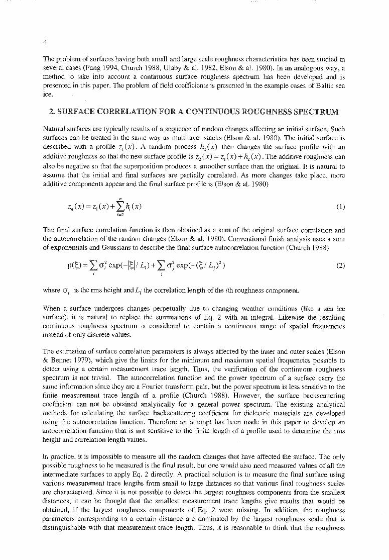
Examples of multiscale surface roughness of Baltic sea ice are shown in Figures 3-6. The spectra have been calculated as ensemble averages of individual measured surface profile spectra and the autocorrelation functions as ensemble averages of individual measured surface profile autocorrelation functions (Church 1988). All these profiles have been measured in three areas of about 100 m x 100 m, except a few small scale profiles in Figure 5, which were situated about 100 m from the rest of the data. Figure 4 represents a many times deformed old ice field in the Bay of Bothnia in 1993 (Manninen, in press, Manninen 1993). The data of Figure 5 was gathered in a huge newly formed netlike ridged area in the Sea of Bothnia in 1994 (Manninen, in press, Manninen 1994). Figure 6 corresponds to a very smooth old level ice field that was situated in the Gulf of Finland in 1994 (Manninen, in press, Manninen 1994).
The spectra of all the three studied ice surfaces are closer to those of fractal than conventional surfaces in the whole studied range (Church 1988). The multiscale autocorrelation functions of Eqs. 12-15 do not have analytical Fourier transforms, but numerical studies showed that these autocorrelation functions produce power spectra, whose slope magnitude decreases both at small and large spatial frequencies, which is observed in all the three sea ice cases (Fig. 3).
In order to compare how well one and multiscale autocorrelation functions approximate the experimental curve, the deviation area between the experimental curve and the approximative functions from origin to correlation length has been calculated. The smaller the ratio of the multiscale area to the one scale area is, the superior the multiscale autocorrelation function is. This deviation area ratio varies from 0.48 to 2.14 for the exponential surface correlation cases of Figs. 4-6. When the multiscale surface correlation of the small scale case of Fig. 6 is changed into transformed exponential surface correlation, the deviation area ratio of multiscale and one scale functions varies from 0.42 to 0.98. Thus, the shape of a multiscale autocorrelation function gives in every case a better alternative than an ordinary one scale function for the studied small, medium and large scale cases. However, it is more important that the multiscale parameters obtained from the medium and large scale measurements produce reasonable autocorrelation functions for the small scale cases (Figs. 4-6). The slight difference is probably partly caused by the small number of profiles in the ensembles and also by the different measurement techniques. The small scale profiles were continuous 1 m long curves digitized with an increment of 1 mm, but the medium scale profiles consisted of 100 discrete points with an increment of 5 cm and the large scale profiles of 100 discrete points with an increment of 50 cm. The multiscale autocorrelation curves proved to be successful also for other studied large scale sea ice types, because they decrease more steeply close to the origin than the corresponding single scale exponential curves.

0.01
E 2 ~
-10
11
rough
large scale
large scale
smooth
small scale
0.01
-8 1. 10
4U
0.1
10. 100. 1000.
frequency (1/m)
t1O 0.1 1 10.
frequency (1/m)
100. 1000.
Figure 3. The spectra of measured large, medium and small scale profiles of rough and smooth Baltic sea ice. The solid curves of rough sea ice represent a many times deformed old ice field in the Bay of Bothnia in 1993
(Churchhouse 1981, Manninen & Rantasuo 1993). The medium scale experimental curve is an ensemble average of seven 5 m long individual profiles. The small scale experimental curve is an ensemble average of 24 individual 0.9 m long profiles. The dashed curves of rough sea ice represent a netlike ridged newly formed ice field in the Sea of Bothnia in 1994 (Manninen, in press, Manninen 1994). The large scale experimental curve
is an ensemble average of four 50 m long individual profiles. The small scale experimental curve is an ensemble average of 17 individual 0.9 m long profiles. The smooth sea ice curves represent an old level ice
field in the Gulf of Finland in 1994 (Manninen, in press, Manninen 1994). The large scale experimental curve is an ensemble average of six 50 m long individual profiles. The small scale experimental curve is an ensemble average of 18 individual 0.9 m long profiles. The number of profiles included in the small scale ensembles is
smaller than was measured, to include only profiles of equal length.

0.8
0
g 0.6
0
~ 0.4 ö U
0.2
12
-0.2
corr
e lat
ion
func
tion
0.8
0.6
0.4
0.2
experimental
multiscale exponential - - - - - -
one scale exponential
medium scale
20 40 60 80 100
distance (cm)
experimental multiscale exponential one scale exponential
medium multiscale exponential
small scale
2
4 6
8
10
distance (cm)
Figure 4. The measured and calculated medium and small scale autocorrelation functions of a many times deformed old ice field in the Bay of Bothnia in 1993 (Churchhouse 1981, Manninen & Rantasuo 1993). The
medium scale experimental curve is an ensemble average of seven 5 m long individual profiles. The small scale experimental curve is an ensemble average of 24 individual 1 m long profiles. The multiscale autocorrelation function calculated for the 1 m distance, using the medium scale surface roughness parameters is also shown
for comparison.
The small scale curves are not quite as clearly exponential as those of medium or large scale, because some of the individual profiles were closer to a Gaussian or transformed exponential type. Yet only the very smooth level ice is better described with a multiscale transformed exponential than the ordinary exponential surface correlation. However, the rounding of the autocorrelation function at the origin can also be an artifact caused by the finite profile length (Church 1988). The stylus wheel diameter used in the small scale measurements was 1 cm, which probably artificially increased the closest correlations.
0.8
experimental multiscale exponential one scale exponential
200 800 600 400 1000
large scale
0.2
experimental multiscale exponential - - - - one scale exponential
large multiscale exponential
S 0.4 -
0.8
-° 0.6 U C
distance (cm)
small scale
13
-0.2 2
4
6
8
10
distance (cm)
Figure 5. The measured and calculated large and small scale autocorrelation functions of a netlike slightly ridged newly formed ice field in the Sea of Bothnia in 1994 (Manninen, in press, Manninen 1994). The large
scale experimental curve is an ensemble average of four 50 m long individual profiles. The small scale experimental curve is an ensemble average of 24 individual 1 m long profiles. The multiscale autocorrelation function calculated for the 1 m distance, using the large scale surface roughness parameters, is also shown for
comparison.
The Integral Equation Method for calculating surface backscattering can be applied to a wide scale of surface roughness, if the surface is random Gaussian and stationary. For Baltic sea ice these two conditions seem to be justified (Haggren & al. 1995). The same equations can be used for cases smaller than the wavelength, comparable to it and larger than it.

-0.2 2 4 6 8 10
1
experimental multiscale exponential - - - -one scale exponential
large multiscale exponential
small scale
0.8
U° • 0.6 C
14
0.8 C 0
experimental
multiscale exponential
one scale exponential
= 0.6 C 0 (7, 0.4 ö U
0.2
0 large scale _
200
400 600
800
1000
distance (cm)
distance (cm)
experimental
multiscale transformed exponential one scale transformed exponential
small scale
2
4
6
8
10
distance (cm)
Figure 6. The measured and calculated large and small scale autocorrelation functions of a very smooth old level ice field in the Gulf of Finland in 1994 (Manninen, in press, Manninen 1994). The large scale
experimental curve is an ensemble average of six 50 m long individual profiles. The small scale experimental curve is an ensemble average of 24 individual 1 m long profiles. The multiscale autocorrelation function
calculated for the 1 m distance, using the large scale surface roughness parameters, is also shown for comparison.
0.8
c o 0.6
ö 0.4
0
-0.2

0 small scale
medium scale
0 0 000
J 0 0
0
-10
cc? -30 E • _ cr)
-40
-50
-60
15
The problem of using the Integral Equation Method of one scale surface roughness for sea ice is clarified in Figure 7. The backscattering coefficient has been calculated using measured surface roughness parameter values corresponding to various lengths within the small and medium scale profiles. Since the rms height and correlation length increase with measurement trace length, the backscattering constant varies also with distance. Moreover the surface roughness parameters do not generally saturate within a few metres. On the contrary there are cases, when they do not saturate even within 100 m (Manninen, in press). It is really difficult to decide, which backscattering coefficient value of Figure 7 (or a value larger than these) one should choose for simulating the backscattering caused by the ERS-1 SAR, whose wavelength is about 5.7 cm and pixel size roughly 25 m. Even the ensemble average would not solve the problem of a backscattering coefficient that continuously increases with the size of the area included in the calculation. Usually it is thought that the roughness scale close to the wavelength used is the most important, but there is no rule on how to choose the exact roughness value to be used.
1
10 100
1000 distance (cm)
Figure 7. Surface backscattering coefficients calculated using ordinary one scale IEM and measured rms height and correlation length values of the many times deformed old ice field of Figure 3. All measurements have been
carried out in an area of 100 m x 100 m. The distance is the radius of the area included in the calculations.
Since the application of IEM taking into account only one roughness scale is problematic, it is useful to check how the inclusion of all roughness scales changes the situation. Figures 8 and 9 show the difference between the backscattering coefficients calculated using the ordinary IEM equations (Fung 1994) and the multiscale IEM based on Eq. 27. The defoi,iied ice field of Figure 8 is an example, where the multiscale surface roughness has a destructive effect on the backscattering even in large distances, whereas the multiscale roughness increases the backscattering for most of the ice types in Figure 9. Basically, the backscattering coefficient varies with increasing distance the same way as in Figure 8. Only the intensity level and the steepness of the curve vary.
Clearly the inclusion of all roughness scales has a slightly destructive effect on the surface autocorrelation function for all studied autocorrelation types (Fig. 1). The net effect on the backscattering coefficient is also negative for the smallest distances, because of the shape of the oscillating integral of Eqs. 25-28. However, the multiscale backscattering increases more strongly with increasing distance than that of the ordinary IEM and surpasses the one scale backscattering for many ice types already in an area having a diameter of about 50 m (Fig. 9). These results have been obtained using the isotropic exponential surface correlation and the comparison has been made using for

O one scale IEM
e multiscale IEM
c=0.949 b=0.267
- k0=0.073
VV • one scale IEM
• multiscale IEM
c=0.949 0=0.267
- k0=0.073
16
multiscale calculations maximum distances that produce the observed correlation length values (Fig. 2). It is natural that the difference between the single and multiscale results is smallest for the smoothest surfaces. The destructive effect of the multiscale exponential surface correlation of Eq. 13 extends up to larger distances, because it neglects a large part of the spherically symmetric surface correlation of Eq. 14. The isotropic exponential surface correlation is understandably more characteristic of natural surfaces than the mathematically more simple quadrangular exponential.
0
H H -5
-10
13
9 -15 E cy) •(7)
-20
-25
-30 0.1
0
-5
-10
03 -o -15
E Co
-20
-25
-30 0.1
lo 100
10 100
1 distance (m)
1
distance (m)
Figure 8. The surface backscattering coefficient of horizontal and vertical polarization calculated for the many times deformed ice field where the medium scale roughness measurements were carried out in 1993
(Churchhouse 1981, Manninen & Rantasuo 1993, Fig. 7). IEM has been applied to single scale or multiscale surface roughness with the isotropic exponential autocorrelation function. The distance is the radius of the area
included in the backscattering calculations. The Kirchhoff and complementary field coefficients have been approximated with the radar incidence angle. The roughness parameter c corresponding to Eq. 7 is given using
cm units for the distance.

• very smooth
o smooth
• slightly deformed
• deformed
o slightly ridged
A ridged
A heavily ridged
0
A A
A HH
A 25 m
0 ~ ...
co -10 E ~
w -20
aa
8 -30
E 40 L-
-40 -30 -20 -10 0
one scale IEM sigma() (dB)
17
o ® o off,
E-15 ° co
w -25 a)
A ®® /
~ -35 ® ~ ~ VV »~ 25 m E j
-45 -45 -35 -25 -15 -5
one scale IEM sigma() (dB)
Figure 9. The surface backscattering coefficient of horizontal and vertical polarization calculated for various large scale ice types measured in 1994 (Manninen, in press, Manninen 1994). IEM has been applied to single scale or multiscale surface roughness with the isotropic exponential autocorrelation function. The Kirchhoff
and complementary field coefficients have been approximated with the radar incidence angle. The calculations are made for an area with a radius of 25 m.
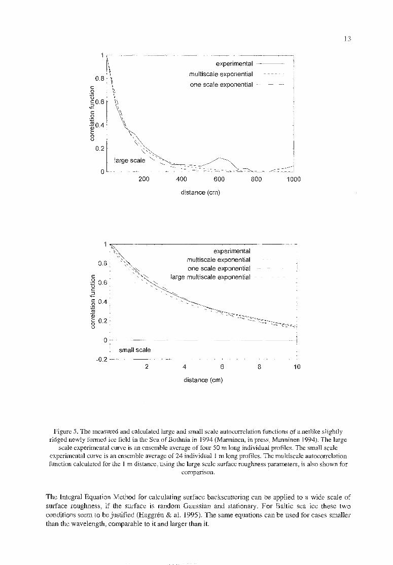
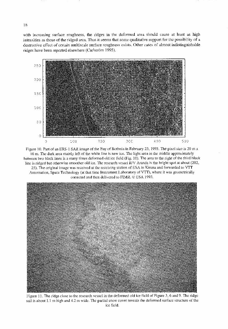
Usually increasing surface roughness leads to increasing backscattering. For example ice ridges are typically distinguished as curvilinear features of higher intensity values in SAR images. However, one example of an indistinguishable ridge is shown in the ERS-1 SAR image of Figure 10. The image consists of the many times deformed old ice area of Figures 7 and 8 (Fig. 11), a smoother ridged old ice field and a new ice area. Although there was a long ridge serpentine roughly parallel to North about 400 m from the research vessel eastwards, it is difficult to see any such feature in the SAR image. Yet the ridge was on average 1.1 m high and 4.2 m broad, which is at least the average size of ridges in the Baltic Sea (Manninen 1996). It is much easier to detect ridges of equal size in the old ice area having a smoother background (Fig. 11). The problem is not only that the average intensity of the deformed ice field is so high that it masks the ridges (Fig. 12), but the maximum intensity values are really smaller in the deformed area than in the ridged area. Since the sample areas are in the same SAR image, the effect can not be explained with calibration errors or the unfavourable incidence angle of ERS-1. Also, the size of the ridges was not typically smaller in the defoiuied area than in the ridged area and the ice of these two areas was equally old and originally similar. The temperature was well below zero during the satellite overpass and the snow cover was only partial (Fig. 11). If the backscattering always increased
250
200
150 -
100
50
18
with increasing surface roughness, the ridges in the deformed area should cause at least as high intensities as those of the ridged area. Thus it seems that some qualitative support for the possibility of a destructive effect of certain multiscale surface roughness exists. Other cases of almost indistinguishable ridges have been reported elsewhere (Carlström 1995).
0 100 200 300 400 500
Figure 10. Part of an ERS-1 SAR image of the Bay of Bothnia in February 23, 1993. The pixel size is 20 m x 16 m. The dark area mainly left of the white line is new ice. The light area in the middle approximately
between two black lines is a many times deformed old ice field (Fig. 10). The area to the right of the third black line is ridged but otherwise smoother old ice. The research vessel R/V Aranda is the bright spot at about (202,
25). The original image was received at the receiving station of ESA in Kiruna and forwarded to VTT Automation, Space Technology (at that time Instrument Laboratory of VTT), where it was geometrically
corrected and then delivered to FIMR. © ESA 1993.
Figure 11. The ridge close to the research vessel in the deformed old ice field of Figure 3, 6 and 9. The ridge sail is about 1.1 m high and 4.2 m wide. The partial snow cover reveals the deformed surface structure of the
ice field.

50 100 150
ridged ice
deformed ice
~_.
0.03
0.01
0.04 new ice
19
200 250
pixel value
Figure 12. The pixel value distributions of the three areas in the ERS-1 SAR image marked in Figure 9.
Although the qualitative behaviour of the multiscale surface roughness combined with the IEM is mostly acceptable, the quantitative results of the very rough ice types do not seem to be high enough. The multiscale treatment produces, at large distances, higher values than the ordinary IEM, but the backscattering level is still too low. The roughness of about the size of the wavelength used is reported to be the most important from the point of view of backscattering (Fung 1994), but the smallest roughness scale does not dominate in Eqs. 2-5. However, it is well known that SAR images are sensitive to the degree of large scale deformation of ice fields. Therefore the larger roughness scales can not be excluded, when simulating the backscattering from sea ice. The problem of taking properly into account the large scale surface roughness is due to the limitations of validity of the Integral Equation Method as will be described in the following analysis.
The necessary condition for the rms slope to guarantee the validity of IEM is (Fung & Chen 1992)
-1264 < 0.3 (29)
where o is the rms height and L the correlation length of the surface. Another criterion for validity of IEM is required for dielectric surfaces when the local incidence angle of the Fresnel reflection coefficients is approximated with the radar incidence angle. For exponential surface correlation the validity is guaranteed when the following relationship for the surface and material parameters and frequency is valid (Fung 1994)
k 26L < 1.6 ~~ (30)
where k is the wave number and Er is the relative peimittivity of the surface. Nevertheless, it is possible that IEM is valid even for larger values of o and L.
For surfaces of multiscale roughness, like Baltic sea ice, Eqs. 23 and 24 actually define the maximum dimension of the area for which the IEM is guaranteed to be applicable. Combining them with Eqs. 6 and 7 we get
x<
i
( 0. 3k0
\ -\Ec ~ (31)

b+E
k 2cko ) (32)
for Eqs. 29 and 30 respectively. The latter condition is for Baltic sea ice, in most cases, more restrictive than the fainter one. The maximum dimensions calculated for measured surfaces using Eqs. 31 and 32 are given in Table 1. The ERS-1 SAR frequency 5.3 GHz was used to calculate the wave number. The permittivity was taken to be 3.15, which is a common value for Baltic sea ice.
Table 1. The criteria for the validity of IEM calculations for measured Baltic sea ice surfaces. The frequency used is 5.3 GHz, the radar incidence angle 23° and the permittivity 3.15. The average value, standard deviation and median of the local incidence angle are given for surfaces measured with a horizontal increment of 50 cm.
maximum length of validity
(m)
local incidence angle (Degrees)
surface type rms slope condition
dielectric condition
median average standard deviation
very smooth 0.34 2.90 23.0 23.0 0.95
very smooth 30.56 0.04 23.0 23.0 0.98
very smooth 10.58 0.04 23.0 23.0 0.46
smooth 15.63 0.80 23.0 23.0 2.56
smooth 2.86 0.09 23.0 23.1 3.45
slightly deformed 0.43 0.35 23.0 23.0 2.67
slightly deformed 0.39 0.25 23.0 23.0 3.54
deformed 1.55 0.10 23.0 23.0 5.10
slightly ridged 2.85 3.68 22.9 23.3 9.29
slightly ridged 0.99 0.90 22.9 22.9 6.84
ridged 37.70 0.03 23.1 24.3 10.7
heavily ridged 4.73 0.90 23.5 26.8 18.1
heavily ridged 3.47 0.66 23.3 25.7 16.5
heavily ridged 14.74 0.11 26.2 33.3 22.5
heavily ridged 31.46 0.09 21.6 23.9 17.4
heavily ridged 35.21 0.06 26.3 29.7 20.7
The validity of IEM clearly varies quite remarkably for the surfaces measured. Still, it seems that in many cases IEM could be applied to areas comparable for example to the resolution of ERS-1 SAR, if the local incidence angle of the Fresnel reflection coefficients can be approximated with a better value than the radar incidence angle.
The effect of the varying local incidence angle has been studied by calculating separately the Kirchhoff coefficients f pp and the complementary field coefficients Fpp for all individual local incidence angles
corresponding to two successive measured surface heights along the 50-100 m long surface roughness measurement lines (Manninen, in press). The statistics of the local incidence angles and these parameters are given in Tables 1-3. It is obvious that even a small variation of the local incidence angle may cause a large change in the values of the field coefficients. Moreover the difference between the average and median values reveal that a few large local incidence angles may dominate the average value of the field coefficients and thus also the backscattering coefficient which is directly proportional to these. For horizontal polarization the field coefficients are monotonous and increase with increasing
20
'C G

21
local incidence angle. For vertical polarization the effect of increasing the local incidence angle is more complicated and may increase or decrease the field coefficients.
Table 2. The average values, standard deviations and medians of the terms f j 2 , F 2 and Re( f„ F v ) for
measured surfaces of Baltic sea ice corresponding to Table 1.
✓ vv l 2 'FIN 2 Re( fvv F„ ) surface type median average standard
deviation median average standard
deviation median average standard
deviation very smooth 0.300 0.300 0.001 0.141 0.142 0.025 0.206 0.207 0.017 very smooth 0.300 0.300 0.001 0.141 0.143 0.025 0.206 0.206 0.018 very smooth 0.300 0.300 0.001 0.141 0.141 0.012 0.206 0.206 0.008 smooth 0.300 0.300 0.004 0.141 0.154 0.087 0.206 0.209 0.047 smooth 0.300 0.300 0.006 0.141 0.163 0.123 0.206 0.212 0.058 slightly deformed 0.300 0.300 0.006 0.141 0.157 0.128 0.206 0.209 0.050 slightly deformed 0.300 0.299 0.007 0.141 0.166 0.147 0.206 0.210 0.066 deformed 0.300 0.298 0.010 0.141 0.195 0.205 0.206 0.217 0.096 slightly ridged 0.301 0.290 0.039 0.138 0.454 1.349 0.204 0.234 0.166 slightly ridged 0.301 0.296 0.019 0.138 0.250 0.439 0.204 0.222 0.130 ridged 0.300 0.284 0.052 0.144 0.792 2.808 0.206 0.238 0.203 heavily ridged 0.300 1.232 8.907 0.153 22.22 168.3 0.183 -4.227 38.74 heavily ridged 0.301 0.445 1.774 0.150 6.410 43.90 0.180 -0.697 8.882 heavily ridged 0.300 1.656 5.129 0.244 39.06 122.5 0.132 -7.000 25.28 heavily ridged 0.302 0.265 0.073 0.108 1.549 3.793 0.166 0.266 0.321 heavily ridged 0.541 2.260 18.77 11.46 56.34 454.0 -1.362 11.37 0.821
Reliable determination of the Fresnel reflection coefficients for materials with low dielectric constant values is not easy, since the determination of the local incidence angle depends crucially on the chosen horizontal increment between the successive surface heights. The values presented in Table I are rather moderate, since the distance was 50 cm. On the other hand, they represent the aerial statistics well, because the length of each line is 50-100 m. Similar analysis of small scale surface roughness measurements showed, that the average values of the local incidence angle, and thence also, the values of the terms involving field coefficients vary remarkably, when the statistic is calculated for intervals of 10 cm, 5 cm, 5 mm and 1 mm from the 1 m long measurement lines (Fig. 13). In practice, it is not possible to measure very long distances with such small intervals. Therefore the results do not then represent a large area very reliably. The calculation of the field coefficients is a question that requires further investigation.
Although the backscattering level in Figures 8 and 9 is not reliable (Table 1, Eqs. 31 and 32), the general shape of the curve in Figure 8 is reasonable, if the ensemble average of the field coefficients does not vary strongly with changing distance. Moreover the difference between the one scale and multiscale cases should not depend very strongly on the field coefficients.

—+~-- Abs[fvv]A2
--+~--- Abs[fhh]A2
22
1
0.8
ru 0 6 a)
0.4
0.2
0 0.1 1 10 100
horizontal increment (mm)
1000
1000 1 10 100
horizontal incr mon (mm)
aver
age
valu
e
--*-- Abs[Fvv]A2
0.5
U
2~ -O5 �
~ ~ ~ ~ ~ > • -1.5
-2
-2.5 0.1 1 10 100
1000
horizontal increment (mm)
o Re[fw*Fw]
--~-- Ro[fhh*Fhh]
Figure 13. The effect of the size of the horizontal increment to the average values of the field coefficient 2 2 ,/ \
parameters a) f , b) /~ and c) |~e\f ~—/~ /nucd~dtbr the backscattering coefficient. The calculations
have been made for 1 m long profiles of small scale roughness measurements digitized with an increment of 1 mm. Therefore, the number of points included in the average values varies between 1000 and 10. Values for
these parameters, corresponding to the approximation of local incidence angle with the radar incidence angle 23°, are a) 0 30 (vv), 0.441 (hh), b) 0.141 (vv), 0.266 (hh), c)O.2O6(vv) and 'A.342 (hh).

23
Table 3. The average values, standard deviations and medians of the terms I fhh 2' Fhh
2 and Re( fhhFhh ) for
measured surfaces of Baltic sea ice corresponding to Table 1.
./ hh 2 1 Fhh 2 Re( fhh Fhh )
surface type median average standard deviation
median average standard deviation
median average standard deviation
very smooth 0.441 0.442 0.013 0.265 0.268 0.049 -0.342 -0.343 0.036 very smooth 0.441 0.442 0.013 0.265 0.269 0.049 -0.342 -0.344 0.036 very smooth 0.441 0.441 0.006 0.265 0.266 0.023 -0.342 -0.342 0.017 smooth 0.441 0.445 0.038 0.265 0.293 0.179 -0.342 -0.354 0.109 smooth 0.441 0.448 0.050 0.265 0.313 0.258 -0.342 -0.363 0.145 slightly deformed 0.441 0.446 0.047 0.265 0.300 0.278 -0.342 -0.356 0.140 slightly deformed 0.441 0.448 0.058 0.265 0.319 0.312 -0.342 -0.363 0.169 deformed 0.441 0.456 0.083 0.265 0.382 0.433 -0.342 -0.389 0.241 slightly ridged 0.440 0.519 0.347 0.259 1.031 3.449 -0.338 -0.602 1.162 slightly ridged 0.440 0.470 0.144 0.259 0.514 0.998 -0.338 -0.434 0.440 ridged 0.443 0.599 0.648 0.271 1.921 7.463 -0.346 -0.879 2.273 heavily ridged 0.448 3.340 18.83 0.289 43.50 294.7 -0.360 -11.59 74.57 heavily ridged 0.446 1.482 6.206 0.283 14.62 94.14 -0.355 -4.251 24.23 heavily ridged 0.490 6.212 16.88 0.470 85.60 258.4 -0.480 -22.64 66.19 heavily ridged 0.423 0.775 0.886 0.201 3.835 10.06 -0.292 -1.484 3.094 heavily ridged 2.357 8.006 63.67 26.51 121.4 966.8 -7.520 31.26 -3E-07
5. DISCUSSION
The radar return of a target depends on the backscattering integrated over individual pixels. The rms height, the autocorrelation function and average local incidence angle of an illuminated pixel characterize the pixel statistically from the point of view of backscattering. The rms height affects strongly the intensity level of the backscattering coefficient. The teiuts of the backscattering coefficient involving the rms height of the surface decrease with increasing rms height for large values of o (Fung 1994). Moreover, the spectrum for the surface correlation (Eqs. 25-28) increases with increasing correlation length. Therefore, without the field coefficients the net effect would be a decrease of the backscattering coefficient with an increase of the surface roughness. This is in contradiction with generally made observations of SAR images. Unfortunately, the field coefficients really seem to have an important role in the surface backscattering calculations of materials of low permittivity, but the reliable estimation of the magnitude of these parameters is very difficult.
It is obvious that the approximation of the local incidence angle with the radar incidence angle (or zero angle) is not always well justified for very rough surfaces. This might be one reason for the problem that in some cases the calculated backscattering coefficient has deviated remarkably from the measured one. It has often been suspected that this is a calibration problem of the measurements or due to a wrong value of the dielectric constant (Fung & Chen 1992, Evans & al. 1992). The approximation of the local incidence angle in the field coefficients with measured values instead of the radar incidence angle often poses the ill defined problem of determining the derivative of a fractal surface.
The approximation of the field coefficients plays an important role in the backscattering calculations. Unfortunately their approximation using the radar incidence angle value for the local incidence angles severely limits the validity of IEM for rough, low permittivity surfaces like Baltic sea ice (Table 1). This is evident also from the results of Figure 9, which show a systematic decrease in backscattering

24
level with an increase of surface deformation, which is in contradiction with general observations. It seems that the high rms height values dominate the results, which are quite sensitive to the exact values of the surface roughness parameters. In conclusion, IEM is not yet applicable to large pixels of very rough surfaces with low permittivity values like Baltic sea ice. Small laboratory samples with salinity resembling that of Arctic sea ice (which is roughly 10 times larger than that of Baltic sea ice) have been successfully modelled using IEM (Beaven & al. 1995, Bredow & al. 1995). The multiscale surface roughness of natural sea ice can be taken into account using the autocorrelation functions presented here, but further research of estimation of the field coefficients and of the effect of large rms height values is required. This will hopefully relax the strict limitations of validity for this excellent theory.
The correlation length of surface heights relatively increases and the rms height decreases with increasing smoothness. In analogy, one may think that a large spatial correlation length of the backscattering coefficient combined with a small amplitude of its variation corresponds to a smooth surface, whereas a larger amplitude represents a rough surface. One might expect for Baltic sea ice that the interdependence of the backscattering coefficient nns height and correlation length is fractallike.
6. SUMMARY AND CONCLUSIONS
Autocorrelation functions describing surfaces with a continuous roughness spectrum have been derived. Multiscale autocorrelation functions were found to approximate corresponding experimental curves of Baltic sea ice better than the ordinary single roughness scale autocorrelation functions. A multiscale surface description makes it easy to study the properties of a surface without having to fix in advance the exact wavelengths of interest.
Equations taking into account multiscale surface roughness, when calculating the surface backscattering coefficient, have been developed. The results shown correspond to surfaces, where all individual roughness components have the same type of autocorrelation function and the same characteristic roughness parameters. The relationship between the roughness parameters and the distance is similar to that of fractallike surfaces. The results can easily be generalized to surfaces of piecewise homogeneous roughness characteristics. The method can also be applied to other types of surfaces with a continuous roughness spectrum, if only the dependence of rms height and correlation length for the distance is known.
The problem of multiscale surface roughness, typical of natural surfaces like sea ice, can be taken into account applying the method presented here, when using IEM for backscattering modelling. The problem that still requires further research is how to estimate the local incidence angles of the field coefficients. In the case of Baltic sea ice, it turned out that the determination of these parameters from measured surface heights is subject to large uncertainty. On the other hand, the use of the radar incidence angle instead of the local incidence angle severely limits the validity of IEM, when the target in question is rough and has a small dielectric constant. Because of the field coefficient approximation IEM is mostly not suitable for large pixels of targets with multiscale surface roughness and small dielectric constant values like Baltic sea ice, although it seems to be applicable for smaller laboratory samples of artificial saline ice.
ACKNOWLEDGMENT
This study has been financially supported by the Finnish Board of Navigation and Technology Development Centre (TEKES). The author is grateful to Dr. Einar-Arne Herland from VTT Automation, Space Technology for processing the SAR image of Figure 10.

25
7. REFERENCES
Beaven, S.G., Lockhart, G.L., Gogineni, S.P., Hosseinmostafa, A.R., Jezek, K., Gow, A.J., Perovich, D.K., Fung, A.K. & Tjuatja, S. 1995: Laboratory measurements of radar backscatter from bare and snow-covered saline ice sheets. - Int. J. Remote Sensing vol. 16, no. 5, pp. 851-876.
Bredow, J.W., Porco, R.L., Fung, A.K., Tjuatja, S., Jezek, K.C., Gogineni, S. & Gow, A. 1995: Determination of Volume and Surface Scattering from Saline Ice Using Ice Sheets with Precisely Controlled Roughness Parameters. - IEEE Trans. Geosci. Remote Sensing, vol. GE-33, no. 5, pp. 1214-1221.
Carlström, A. 1995: Modelling microwave backscattering from sea ice for Synthetic-Aperture Radar applications. - Technical Report No. 271, Chalmers University of Technology.
Church, E.L. 1988: Fractal surface finish. - Applied Optics, vol. 27, no. 8, pp. 1518-1526.
Churchhouse, R.F. 1981: Ed., Handbook of applicable mathematics, Vol III, Chichester: John Wiley & Sons.
Elson, J.M. & Bennett, J.M. 1979: Relation between the angular dependence of scattering and the statistical properties of optical surfaces. - J. Opt. Soc. Am., vol. 69, no. 1, pp. 31-47.
Elson, J.M., Rahn, J.P. & Bennett, J.M. 1980: Light scattering from multilayer optics: comparison of theory and experiment. - Applied Optics, vol. 19, no. 5, pp. 669-679.
Evans, D.L., Farr, T.G. & van Zyl, J.J. 1992: Estimates of surface roughness derived from synthetic aperture radar (SAR) data. - IEEE Trans. Geosci. Remote Sensing, vol. GE-30, no. 2, pp.382-389.
Fung, A.K. & Chen, K.S. 1992: Dependence of the surface backscattering coefficients on roughness, frequency and polarization states. - Int. J. Remote Sensing, vol. 13, no. 9, pp.1663-1680.
Fung, A.K. 1994: Microwave scattering and emission models and their applications. - Artech House, Norwood, MA.
Fung, A.K., Li, Z. & Chen, K.S. 1992: Backscattering from a randomly rough dielectric surface. - IEEE Trans. Geosci. Remote Sensing, vol. GE-30, no. 2, pp.356-369.
Gradshteyn, I.S. & Ryzhik, I.M. 1980: Table of integrals, series and products. - Academic Press, New York.
Haggren, H., Manninen, T., Peräläinen, I., Pesonen, J., Pöntinen, P. & Rantasuo, M. 1995: Airborne 3D-profilometer. - VTT Research Notes 1667.
Keller, J.M., Crownover, R.M. & Chen, R.Y. 1987: Characteristics of natural scenes related to the fractal dimension. - IEEE Trans. Pattern Anal. Machine Intell., vol. PAMI-9, no. 5, pp. 621-627.
Manninen, A.T. 1994: Large and small scale sea ice surface topography measurements during 14 - 28 March, 1994. - Finnish Institute of Marine Research Internal Report 1994(12).
Manninen, A.T. 1996: Surface morphology and backscattering of ice ridge sails in the Baltic Sea. - Journal of Glaciology, vol. 42, no. 140, pp. 141-156.
Manninen, A.T.: Problematic calculation of surface backscattering of sea ice. - To be published in Proc. PIERS '94.
Manninen, A.T.: Surface roughness of Baltic sea ice. - Journal of Geophysical Research, Oceans (in press).
Manninen, T. 1993: Mechanical measurements of sea ice surface topography. - Finnish Institute of Marine Research Internal Report 1993(8).

26
Manninen, T. and Rantasuo, M. 1993: Sea ice topography measurements. - Finnish Institute of Marine Research Internal Report 1993(2).
Ulaby, F.T., Moore, R.K. & Fung, A.K. 1982: Microwave Remote Sensing. Vol. II, - Addison-Wesley, Reading, MA.
Wolfram, S. 1991: Mathematica, A system for doing mathematics by computer. - Addison-Wesley, Redwood City, CA.


z 0 N G)
BA
CK
SC
ATT
ER
ING
FRO
M A D
IELE
CTR
IC S
UR
FAC
E W
ITH A
CO
NTIN
UO
US
ROU
GH
NE
SS
SP
EC
TRU
M
Merentutkimuslaitos Lyypekinkuja 3 A PL 33 00931 Helsinki
Havsforskningsinstitutet PB 33 00931 Helsingfors
Finnish Institute of Marine Research P.O.Box 33 FIN-00931 Helsinki, Finland
ISBN 951-53-0800-3 ISSN 1238-5328