surface and volumetric backscattering betwee … code: 0277-786x/14/$18 · doi: 10.1117/12.2051772...

Surface and Volumetric Backscattering Between 100 GHz and 1.6 THz

D. A. DiGiovanni, A. J. Gatesman, T. M. Goyette, and R. H. Giles Submillimeter-Wave Technology Laboratory, University of Massachusetts Lowell, Lowell, MA

01854

ABSTRACT Successful development of remote sensing and communication systems in the terahertz band requires a better understanding of the scattering behavior of various structures. Materials that could be considered homogeneous and smooth at microwave frequencies may begin to display surface and volumetric scattering behavior in the terahertz band. The co-polarization backscattering coefficient of several types of metal and dielectric structures were measured in indoor compact radar ranges operating at 100 GHz, 160 GHz, 240 GHz, and 1.55 THz. These structures consisted of roughened aluminum plates, as well as homogeneous and inhomogeneous dielectric surfaces. The roughness and inclusions of the measured samples were tailored in order to systematically investigate various scattering effects. Polarimetric backscattering measurements of these materials were collected at elevation angles from 5 to 75 degrees. Analysis of the backscatter data supports a better understanding of surface and volumetric scattering behavior of materials at terahertz frequencies. Keywords: rough surface, scattering, terahertz, clutter, millimeter-wave

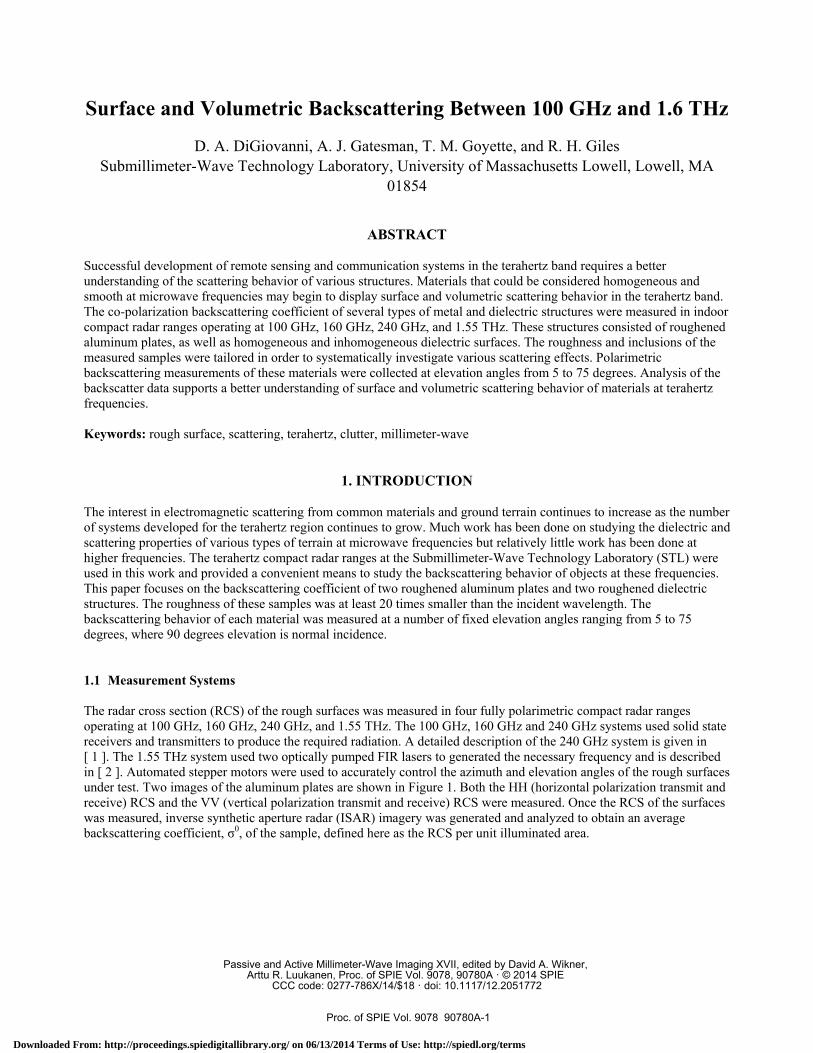
1. INTRODUCTION The interest in electromagnetic scattering from common materials and ground terrain continues to increase as the number of systems developed for the terahertz region continues to grow. Much work has been done on studying the dielectric and scattering properties of various types of terrain at microwave frequencies but relatively little work has been done at higher frequencies. The terahertz compact radar ranges at the Submillimeter-Wave Technology Laboratory (STL) were used in this work and provided a convenient means to study the backscattering behavior of objects at these frequencies. This paper focuses on the backscattering coefficient of two roughened aluminum plates and two roughened dielectric structures. The roughness of these samples was at least 20 times smaller than the incident wavelength. The backscattering behavior of each material was measured at a number of fixed elevation angles ranging from 5 to 75 degrees, where 90 degrees elevation is normal incidence. 1.1 Measurement Systems The radar cross section (RCS) of the rough surfaces was measured in four fully polarimetric compact radar ranges operating at 100 GHz, 160 GHz, 240 GHz, and 1.55 THz. The 100 GHz, 160 GHz and 240 GHz systems used solid state receivers and transmitters to produce the required radiation. A detailed description of the 240 GHz system is given in [ 1 ]. The 1.55 THz system used two optically pumped FIR lasers to generated the necessary frequency and is described in [ 2 ]. Automated stepper motors were used to accurately control the azimuth and elevation angles of the rough surfaces under test. Two images of the aluminum plates are shown in Figure 1. Both the HH (horizontal polarization transmit and receive) RCS and the VV (vertical polarization transmit and receive) RCS were measured. Once the RCS of the surfaces was measured, inverse synthetic aperture radar (ISAR) imagery was generated and analyzed to obtain an average backscattering coefficient, σ0, of the sample, defined here as the RCS per unit illuminated area.

Passive and Active Millimeter-Wave Imaging XVII, edited by David A. Wikner, Arttu R. Luukanen, Proc. of SPIE Vol. 9078, 90780A · © 2014 SPIE

CCC code: 0277-786X/14/$18 · doi: 10.1117/12.2051772

Proc. of SPIE Vol. 9078 90780A-1

Downloaded From: http://proceedings.spiedigitallibrary.org/ on 06/13/2014 Terms of Use: http://spiedl.org/terms

Figure 1. Roughened aluminum plates mounted at 65 degrees and 45 degrees elevation respectively.

2. SCATTERING THEORY Rough surface scattering theory is of great interest to a variety of different fields. Though there has been much work done on developing a rough surface scattering theory that applies to any arbitrary surface and wavelength, current theories are still limited. Rough surface scattering theory can be broken up into three regimes [ 3 ], long wavelength, short wavelength, and a hybrid theory. Since the rms roughness of the measured samples is much smaller than the incident wavelength (s/λ ~ 0.04 and smaller), the theory used for this paper will be in the long wavelength regime [ 4 ], [ 5 ]. The long wavelength regime theory is based on a perturbation technique and has three assumptions about the scattering surface. One, the roughness is small compared to the incident wavelength, i.e. ks is less than 1. Two, the surface slopes are small and are expressed mathematically as ⏐∂H/∂x⏐ and ⏐∂H/∂y⏐ being less than 45 degrees. Three, the roughness is isotropic. Table I shows that the samples satisfy the first two assumptions. Since there was no azimuthal dependence in the measured RCS, the last assumption was also assumed to be satisfied. The theory was developed to work for bistatic scattering but can easily be applied to backscatter measurements by setting the scattering angles θincident = θscattered and φscattered = 180 degrees. The average incoherent backscattering cross section per unit projected area is given by equation ( 1 ). σ pq

0 = 4π k0

4s2 cos4θi α pq2

I ( 1 )

P and q are the scattered and incident polarization states, respectively, θi is the incident angle of the beam, αpq is a scattering function based on the materials relative dielectric constant εr and the scattering angle, and I is a function derived from the autocovariance function C(τ). For the measured materials, the Gaussian form of exp(-τ2/L2) was assumed to be an adequate fit to the measured C(τ). I will then be given by equation ( 2 ). I = πL2 exp(−k0

2L2 sin2θi ) ( 2 ) The scattering function α can be written in terms of either linear or circular polarization states. Measurements for this study were taken with linear polarization states with the electric field either parallel to the plane of incidence (vertical polarization) or perpendicular to the plane of incidence (horizontal polarization). The equations for αpq for non magnetic materials in the backscattering case are given by ( 3 ) and ( 4 ).

αHH = 1−εr

(cosθi + εr − sin2θi )2 ( 3 )



αVV =

(εr −1)[(εr −1)sin2θi +εr ](εr cosθi + εr − sin2θi )2

( 4 )

It should be noted that, according to this theory, the cross polarization states of αHV and αVH are zero for the backscattering case. This contradicts with some experimental observations [ 6 ]. Equations ( 3 ) and ( 4 ) can be simplified to describe the scattering of perfect conductors by taking the limit of εr as it approaches infinity. In this case, αHH and αVV are reduced to the following equations. αHH =1 ( 5 )

αVV =1+ sin2θi

cos2θi

( 6 )

The difference between equations ( 3 ) and ( 4 ) to equations ( 5 ) and ( 6 ) becomes noticeable when εr is small or θi approaches grazing angles. For large, but finite, values of εr, such as those expected for metals at terahertz frequencies, equations ( 5 ) and ( 6 ) can be used as a good approximation. By substituting equations ( 2 ), ( 5 ), and ( 6 ) into equation ( 1 ), the resulting backscattering coefficients of metals for HH and VV polarizations are, σ HH

0 = 4k04s2L2 cos4θi exp(−k0

2L2 sin2θi ) ( 7 ) σVV

0 = 4k04s2L2 (1+ sin2θi )

22 exp(−k02L2 sin2θi ) ( 8 )

It is important to note that the cosn dependence, observed in many dielectric measurements [ 7 ] - [ 12 ], disappears in the VV backscattering coefficient for materials with a large εr. According to equation ( 8 ), for k0L around 1 or smaller, σ0

VV will actually be larger at grazing angles compared to normal higher elevation angles. This somewhat counterintuitive result is validated by our measurements. For the inhomogeneous dielectric, there were additional scattering effects expected to contribute to the measured value of σ0. In addition to the surface scattering theory given above, there was also the possibility of volumetric scattering. The total backscatter coefficient would then be the sum of two parts, σ0

surface and σ0volumetric. Nashashibi [ 12 ] observed

volumetric scattering in soil only when the incident wavelength was on the order of the diameter of the inclusions. For this study, volumetric scattering was expected to occur for the inhomogeneous dielectric when measured at 1.55 THz. At this frequency, the wavelength was approximately twice the size of the silicon carbide particles (λ ≈ 193 μm, particle diameter ≈ 100 μm).



3. MATERIAL PREPERATION AND CHARACTERIZATION 3.1 Sample Preparation Two different techniques were used to obtain a roughened surface for the measured materials. An industrial sand blaster was used to roughen two 24 inch by 24 inch aluminum plates. Plate 1 was 1/4 inch thick and was roughened using approximately 300 micron sized sand. Plate 2 was 3/8 inches thick and was roughened using approximately 400 micron sized sand. The two plates were washed with water after sandblasting to remove any loose sand. Using the sand blaster on the aluminum did create a slight curve to the plates. Fortunately, the radius of curvature was approximately 900 inches and was assumed to have a negligible impact on the measured RCS. A sample with homogeneous dielectric properties was created using a two part, polyurethane mix. The A and the B part were mixed with 99% pure, -325 mesh, carbon powder. The average particle size of the powder was about 44 microns. The carbon powder was baked at over 100 degrees C for four hours to remove any excess moisture. The amount of carbon powder added was 5% of the mass of the combined part A and B mixture. Once the carbon was thoroughly mixed into each part, the mixture was placed in a vacuum chamber to remove any excess air. After degassing, the two parts were combined and then degassed again. When ready, the sample was poured into an 8 inch silicone mold with the desired surface texture. In addition, smaller test samples were prepared for measurement in a far infrared spectrometer in order to properly calculate the dielectric constant of the carbon loaded plastic. A sample with inhomogeneous dielectric properties was created by adding 5% by mass of silicon carbide powder in addition to the 5% by mass carbon powder to the polyurethane plastic. The average particle size of the silicon carbide was around 100 microns. The diameter of the silicon carbide particles is approximately half the size of the incident wavelength at 1.55 THz. Since the silicon carbide is relatively large, it was expected that internal, volumetric, scattering would now begin to contribute to the total backscattering coefficient. 3.2 Surface Roughness Data Three main parameters commonly measured when studying the roughness of a surface, with a height profile defined by the function H(x,y), are the root mean square (rms) roughness, s, the surface slopes, dq, and the correlation length, L. The rms roughness is an rms average of the heights above or below a mean reference line. The surface slopes are an rms average of the derivative of the measured height profile. The correlation length gives a measure of how far two points must be separated along the mean reference line before their heights are considered uncorrelated. In order to calculate the correlation length, the autocovariance function, C(τ), must first be computed using equation ( 9 ).

C(m *Δx)= 1s2

1N−M (H jj=1

N−M∑ * H j+m );m =1, 2,3,..., M. ( 9 )

Hj and Hj+m are the measured profile heights at discrete points j and j+m, where j=1 was the first point and j=N was the last point of the height profile. The correlation length is then defined as the value where C(L) = e-1 ≈ 0.368. The surface roughness of all of the samples was measured by using a stylus profilometer. A 2 micron diameter conical tip stylus scanned the rough surface and provided a height profile. The value of Δx was 5 microns. The quantities ks and kL, where k is the free space wavenumber 2πf/c, were calculated to give quantifiable values of the roughness to wavelength (s/λ) and correlation length to wavelength (L/λ) ratios. Between 20 and 40 height profile measurements were taken for each sample. From each of these measurements, values of s and L were acquired. The average rms roughness, surface slope, correlation length, ks, and kL values for the materials in this study are shown in Table I and Table II.



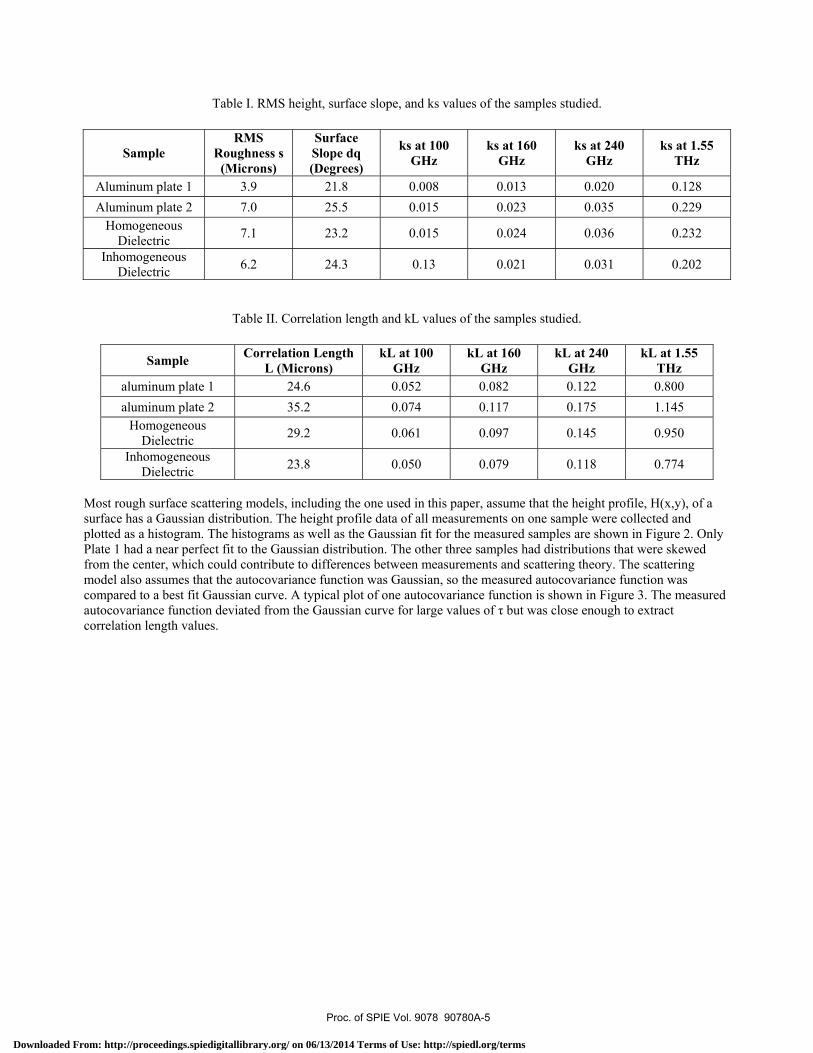
Table I. RMS height, surface slope, and ks values of the samples studied.

Sample RMS

Roughness s (Microns)

Surface Slope dq (Degrees)

ks at 100 GHz

ks at 160 GHz

ks at 240 GHz

ks at 1.55 THz

Aluminum plate 1 3.9 21.8 0.008 0.013 0.020 0.128 Aluminum plate 2 7.0 25.5 0.015 0.023 0.035 0.229

Homogeneous Dielectric 7.1 23.2 0.015 0.024 0.036 0.232

Inhomogeneous Dielectric 6.2 24.3 0.13 0.021 0.031 0.202

Table II. Correlation length and kL values of the samples studied.

Sample Correlation Length L (Microns)

kL at 100 GHz

kL at 160 GHz

kL at 240 GHz

kL at 1.55 THz

aluminum plate 1 24.6 0.052 0.082 0.122 0.800 aluminum plate 2 35.2 0.074 0.117 0.175 1.145

Homogeneous Dielectric 29.2 0.061 0.097 0.145 0.950

Inhomogeneous Dielectric 23.8 0.050 0.079 0.118 0.774

Most rough surface scattering models, including the one used in this paper, assume that the height profile, H(x,y), of a surface has a Gaussian distribution. The height profile data of all measurements on one sample were collected and plotted as a histogram. The histograms as well as the Gaussian fit for the measured samples are shown in Figure 2. Only Plate 1 had a near perfect fit to the Gaussian distribution. The other three samples had distributions that were skewed from the center, which could contribute to differences between measurements and scattering theory. The scattering model also assumes that the autocovariance function was Gaussian, so the measured autocovariance function was compared to a best fit Gaussian curve. A typical plot of one autocovariance function is shown in Figure 3. The measured autocovariance function deviated from the Gaussian curve for large values of τ but was close enough to extract correlation length values.



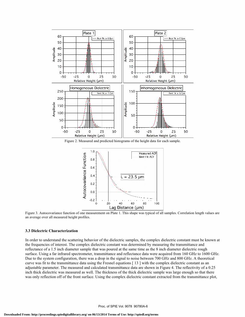
Plate 1 Plate 260

50

40

ff20

0

r_ Best Fit, s =3.BNm60

50

0 40

Q 20

10

0

- Best Fit, s =7.0Nm

-Y1

hi

III10

_-11IÌjIIII I1-_1111Ì1111, _illin111111 IIIIIIIIIIIII1.

-50 -25 0 25 50Relative Height (pm)

-50 -25 0 25 50Relative Height (Nm)

Inhomogeneous DielectricHomogeneous Dielectric250

200

g 150

É 100a

50

0

Best Fit, s= 7.2pm]1 50

100

Éa 50

- Best Fit, s =6.2um

111 II-1F E.-iiII-.iiiiiitI-I1-- ,I 1,íE11111ÌÌÌD! - o-50 -25 0 25 50

Relative Height (pm)-50 -25 0 25 50

Relative Height (pm)

O

1.0

0.8

0.6

0.4

0.2

0.0

0.2o

-- In- Measured ACF

Best Fit ACF

MEIN.

L - 23.5 pm

20 40 60 80

Lag Distance (pm)100

Figure 2. Measured and predicted histograms of the height data for each sample.

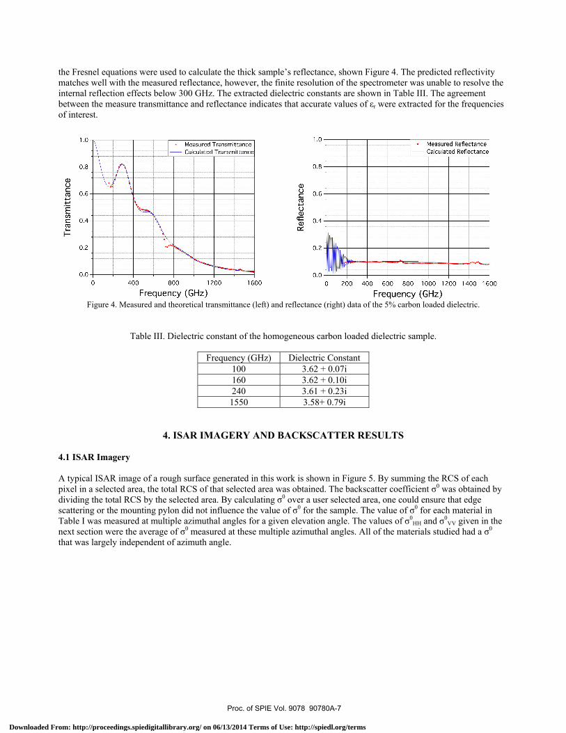
Figure 3. Autocovariance function of one measurement on Plate 1. This shape was typical of all samples. Correlation length values are an average over all measured height profiles. 3.3 Dielectric Characterization In order to understand the scattering behavior of the dielectric samples, the complex dielectric constant must be known at the frequencies of interest. The complex dielectric constant was determined by measuring the transmittance and reflectance of a 1.5 inch diameter sample that was poured at the same time as the 8 inch diameter dielectric rough surface. Using a far infrared spectrometer, transmittance and reflectance data were acquired from 160 GHz to 1600 GHz. Due to the system configuration, there was a drop in the signal to noise between 700 GHz and 800 GHz. A theoretical curve was fit to the transmittance data using the Fresnel equations [ 13 ] with the complex dielectric constant as an adjustable parameter. The measured and calculated transmittance data are shown in Figure 4. The reflectivity of a 0.25 inch thick dielectric was measured as well. The thickness of the thick dielectric sample was large enough so that there was only reflection off of the front surface. Using the complex dielectric constant extracted from the transmittance plot,



1.0

0.8

0.6

0.4

0.2

0.0

Measured TransmittanceCalculated Transmittance

o 400 800 1200

Frequency (GHz)1600

1.0

0.8

0.6

0.4

0.2

0.00 200 400 600 800 1000 1200 1400 1600

Frequency (GHz)

Measured ReflectanceCalculated Reflectance

the Fresnel equations were used to calculate the thick sample’s reflectance, shown Figure 4. The predicted reflectivity matches well with the measured reflectance, however, the finite resolution of the spectrometer was unable to resolve the internal reflection effects below 300 GHz. The extracted dielectric constants are shown in Table III. The agreement between the measure transmittance and reflectance indicates that accurate values of εr were extracted for the frequencies of interest.

Figure 4. Measured and theoretical transmittance (left) and reflectance (right) data of the 5% carbon loaded dielectric.

Table III. Dielectric constant of the homogeneous carbon loaded dielectric sample.

Frequency (GHz) Dielectric Constant 100 3.62 + 0.07i 160 3.62 + 0.10i 240 3.61 + 0.23i 1550 3.58+ 0.79i

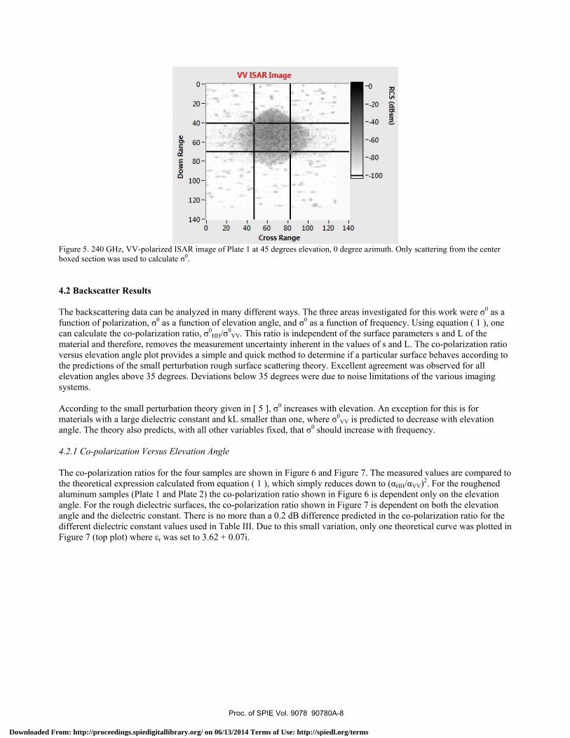
4. ISAR IMAGERY AND BACKSCATTER RESULTS 4.1 ISAR Imagery A typical ISAR image of a rough surface generated in this work is shown in Figure 5. By summing the RCS of each pixel in a selected area, the total RCS of that selected area was obtained. The backscatter coefficient σ0 was obtained by dividing the total RCS by the selected area. By calculating σ0 over a user selected area, one could ensure that edge scattering or the mounting pylon did not influence the value of σ0 for the sample. The value of σ0 for each material in Table I was measured at multiple azimuthal angles for a given elevation angle. The values of σ0

HH and σ0VV given in the

next section were the average of σ0 measured at these multiple azimuthal angles. All of the materials studied had a σ0 that was largely independent of azimuth angle.



0

20

40 -

120 -

VV ISAR Image

- 0

LI

--60

--00

--100

140 -i i i i i' i

0 20 40 60 80 100 120 140

Cross Range

á

Figure 5. 240 GHz, VV-polarized ISAR image of Plate 1 at 45 degrees elevation, 0 degree azimuth. Only scattering from the center boxed section was used to calculate σ0. 4.2 Backscatter Results The backscattering data can be analyzed in many different ways. The three areas investigated for this work were σ0 as a function of polarization, σ0 as a function of elevation angle, and σ0 as a function of frequency. Using equation ( 1 ), one can calculate the co-polarization ratio, σ0

HH/σ0VV. This ratio is independent of the surface parameters s and L of the

material and therefore, removes the measurement uncertainty inherent in the values of s and L. The co-polarization ratio versus elevation angle plot provides a simple and quick method to determine if a particular surface behaves according to the predictions of the small perturbation rough surface scattering theory. Excellent agreement was observed for all elevation angles above 35 degrees. Deviations below 35 degrees were due to noise limitations of the various imaging systems. According to the small perturbation theory given in [ 5 ], σ0 increases with elevation. An exception for this is for materials with a large dielectric constant and kL smaller than one, where σ0

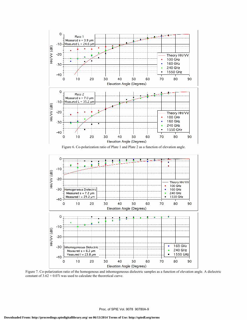
VV is predicted to decrease with elevation angle. The theory also predicts, with all other variables fixed, that σ0 should increase with frequency. 4.2.1 Co-polarization Versus Elevation Angle The co-polarization ratios for the four samples are shown in Figure 6 and Figure 7. The measured values are compared to the theoretical expression calculated from equation ( 1 ), which simply reduces down to (αHH/αVV)2. For the roughened aluminum samples (Plate 1 and Plate 2) the co-polarization ratio shown in Figure 6 is dependent only on the elevation angle. For the rough dielectric surfaces, the co-polarization ratio shown in Figure 7 is dependent on both the elevation angle and the dielectric constant. There is no more than a 0.2 dB difference predicted in the co-polarization ratio for the different dielectric constant values used in Table III. Due to this small variation, only one theoretical curve was plotted in Figure 7 (top plot) where εr was set to 3.62 + 0.07i.



o

-10-

> -20>

Plate 1Measured s = 3.9 pm

Measured L = 24.6 pm

-30

-400 10 20 30 40 50 60

Elevation Angle (Degrees)

Theory HH /VV100 GHz160 GHz240 GHz1550 GHz

1 170 80 90

0-

-30

-400

Plate 2Measured s = 7.0 pm

Measured L = 35.2 pm


10 20 30 40 50 60Elevation Angle (Degrees)

70 80 90

-30-

-400 10 20 30 40 50 60


Homogeneous DielectricMeasured s = 7.2 pmMeasured I = 29.2 pm


170 80 90

o

-400

f

Inhomogeneous DielectricMeasured s = 6.2 pmMeasured I = 23.8 pm

10 20 30 40 50 60 70Elevation Angle (Degrees)

160 GHz240 GHz1550 GHz

80 90

Figure 6. Co-polarization ratio of Plate 1 and Plate 2 as a function of elevation angle.

Figure 7. Co-polarization ratio of the homogenous and inhomogeneous dielectric samples as a function of elevation angle. A dielectric constant of 3.62 + 0.07i was used to calculate the theoretical curve.



0--10--20

-30

-40

-50

-60

-70

F =100 GHzMeasured s =3.9 pm

HH MeasuredVV Measured

Fit L =71 .2 pm - HH Theory- VV Theory

02,...----a-------j

0 10 20 30 40 50 60 70 80 90Elevation Angle (Degrees)

0

-10

-20

-30

-40

-50

-60

-70



Fit L =62.6 pmHH Theory

- VV Theory

, _


o

-10

-20

-30

-40

-50

-60

-70



Fit L =58.3 pm HH Theory- VV Theory


0

-10

-20

-30

-40

-50

-60

-70

HH MeasuredVV MeasuredF=1550 GHz

Measured s =3.9 pmFit L =28.4 pm

HH Theory- VV Theory


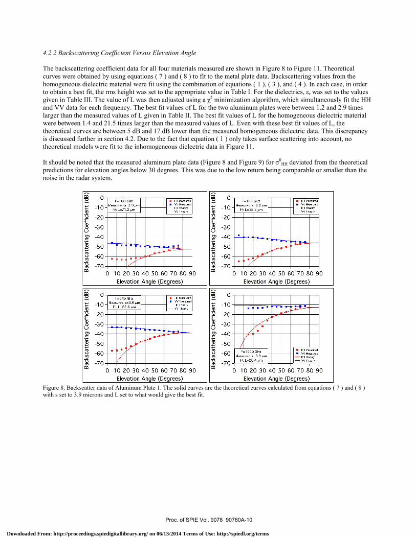
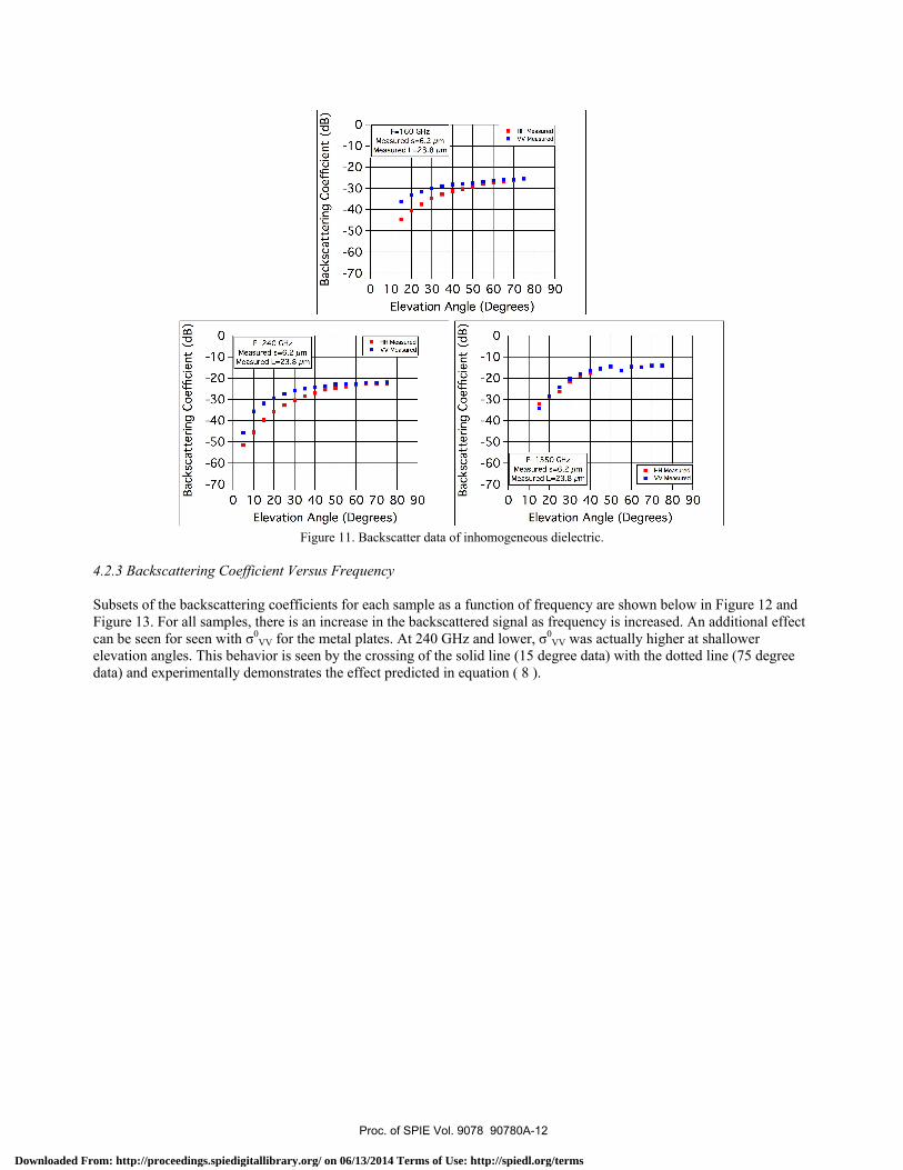
4.2.2 Backscattering Coefficient Versus Elevation Angle The backscattering coefficient data for all four materials measured are shown in Figure 8 to Figure 11. Theoretical curves were obtained by using equations ( 7 ) and ( 8 ) to fit to the metal plate data. Backscattering values from the homogeneous dielectric material were fit using the combination of equations ( 1 ), ( 3 ), and ( 4 ). In each case, in order to obtain a best fit, the rms height was set to the appropriate value in Table I. For the dielectrics, εr was set to the values given in Table III. The value of L was then adjusted using a χ2 minimization algorithm, which simultaneously fit the HH and VV data for each frequency. The best fit values of L for the two aluminum plates were between 1.2 and 2.9 times larger than the measured values of L given in Table II. The best fit values of L for the homogeneous dielectric material were between 1.4 and 21.5 times larger than the measured values of L. Even with these best fit values of L, the theoretical curves are between 5 dB and 17 dB lower than the measured homogeneous dielectric data. This discrepancy is discussed further in section 4.2. Due to the fact that equation ( 1 ) only takes surface scattering into account, no theoretical models were fit to the inhomogeneous dielectric data in Figure 11. It should be noted that the measured aluminum plate data (Figure 8 and Figure 9) for σ0

HH deviated from the theoretical predictions for elevation angles below 30 degrees. This was due to the low return being comparable or smaller than the noise in the radar system.

Figure 8. Backscatter data of Aluminum Plate 1. The solid curves are the theoretical curves calculated from equations ( 7 ) and ( 8 ) with s set to 3.9 microns and L set to what would give the best fit.



0

-10

-20

-30

-40

-50

-60

-70



Fit L =54.8 pm- HH Theory- VV Theory

::::0 10 20 30 40 50 60 70 80 90


0

-10

-20

-30

-40

-50

-60

-70





o

-10

-20

-30

-40

-50

-60

-70



Fit L =52.2 pm- HH Theory- VV Theory

. .0 10 20 30 40 50 60 70 80 90


0

-10

-20

-30

-40

-50

-60

-70





0--10--20

-30

-40

-50

-60

-70




1 I r T

--------

iI.r0 10 20 30 40 50 60 70 80 90


0--10--20

-30

-40

-50

-60

-70




---------

70 10 20 30 40 50 60 70 80 90


0--10--20

-30

-40

-50

-60

-70




1OnFAPEPP

4MÎi.


0

-10

-20

-30

-40

-50

-60 -

-70 -

1 I

PI/'/Iii





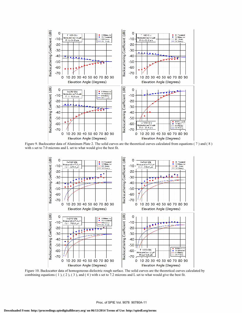
Figure 9. Backscatter data of Aluminum Plate 2. The solid curves are the theoretical curves calculated from equations ( 7 ) and ( 8 ) with s set to 7.0 microns and L set to what would give the best fit.

Figure 10. Backscatter data of homogeneous dielectric rough surface. The solid curves are the theoretical curves calculated by combining equations ( 1 ), ( 2 ), ( 3 ), and ( 4 ) with s set to 7.2 microns and L set to what would give the best fit.



o

-10

-20

-30

-40

-50

-60

-70


Measured L =23.8 pm


' , ,


0

-10

-20

-30

-40

-50

-60

-70


Measured L =23.8 pm


' I N E N


0

-10

-20

-30

-40

-50

-60

-70


Measured L =23.8 pmHH MeasuredVV Measured


Figure 11. Backscatter data of inhomogeneous dielectric.

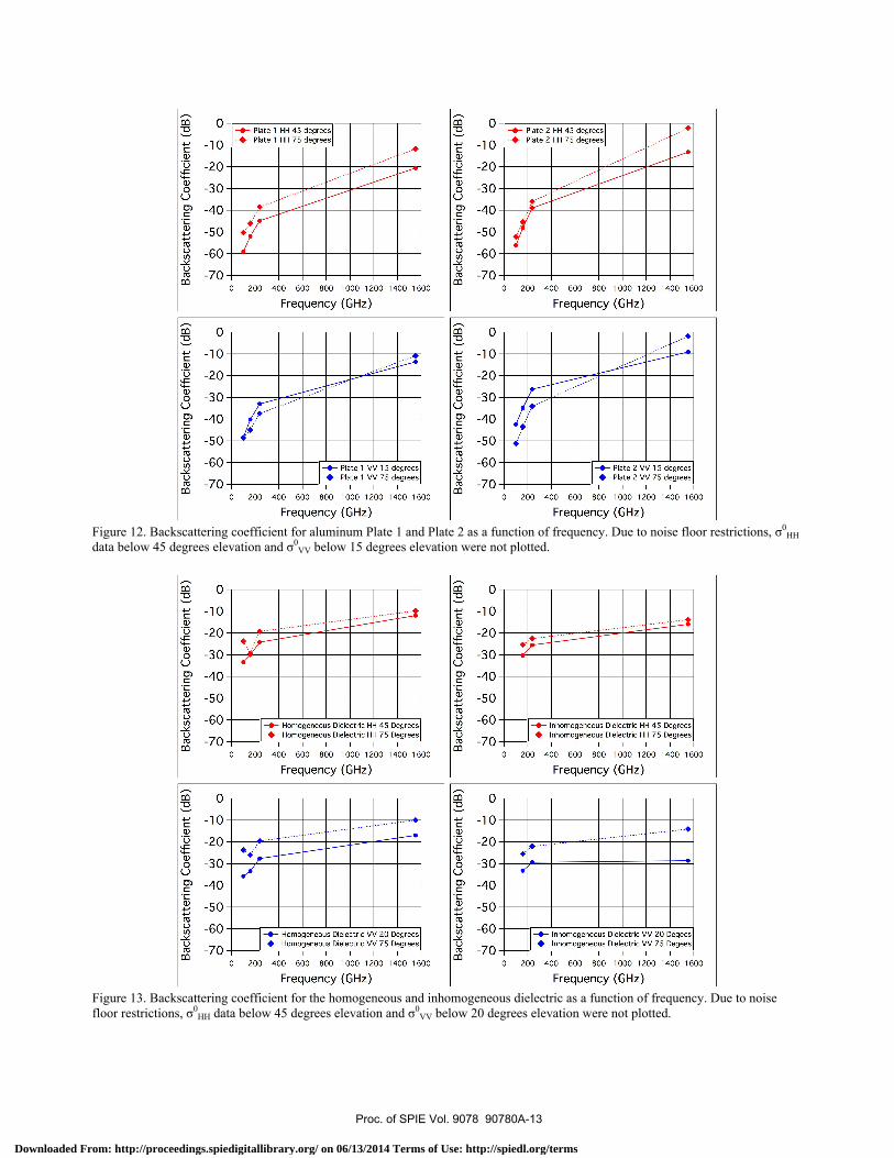
4.2.3 Backscattering Coefficient Versus Frequency Subsets of the backscattering coefficients for each sample as a function of frequency are shown below in Figure 12 and Figure 13. For all samples, there is an increase in the backscattered signal as frequency is increased. An additional effect can be seen for seen with σ0

VV for the metal plates. At 240 GHz and lower, σ0VV was actually higher at shallower

elevation angles. This behavior is seen by the crossing of the solid line (15 degree data) with the dotted line (75 degree data) and experimentally demonstrates the effect predicted in equation ( 8 ).



0--10-

-20

-30

-40

-50

-60

-70o

Plate 1 HH 45 degrees-- Plate 1 HH 75 degrees

200 400 600 800 1000 1200 1400 1600

Frequency (GHz)

0

-10

-20

-30

-40

-50

-60

-70o

i

-- Plate 1 VV 15 degrees-- Plate 1 VV 75 degrees

I I I

200 400 600 800 1000 1200 1400 1600

Frequency (GHz)

0--10-

-20

-30

-40

-50

-60

-70o

-- Plate 2 HH 45 degrees-- Plate 2 HH 75 degrees

200 400 600 800 1000 1200 1400 1600

Frequency (GHz)

0

-10

-20

-30

-40

-50

-60

-70o

Plate 2 VV 15 degrees- - Plate 2 VV 75 degrees

I I I

200 400 600 800 1000 1200 1400 1600

Frequency (GHz)

0

-10

-20

-30

-40

-50

-60

-70o

%

f Homogeneous Dielectric HH 45 Degrees-- Homogeneous Dielectric HH 75 Degrees

I I I I I I

200 400 600 800 1000 1200 1400 1600

Frequency (GHz)

0

-10

-20

-30

-40

-50

-60

-70o

f Homogeneous Dielectric VV 20 Degrees-- Homogeneous Dielectric VV 75 Degrees

I I I I I I

200 400 600 800 1000 1200 1400 1600

Frequency (GHz)

0

-10

-20

-30

-40

-50

-60

-70o

f Inhomogeneous Dielectric HH 45 Degrees-- Inhomogeneous Dielectric HH 75 Degrees

I I I I I I

200 400 600 800 1000 1200 1400 1600

Frequency (GHz)

0

-10

-20

-30

-40

-50

-60

-70o

----------------.----------.-----.----

_____.

-- Inhomogeneous Dielectric VV 20 Degees-- Inhomogeneous Dielectric VV 75 Degees

I I I I I I

200 400 600 800 1000 1200 1400 1600

Frequency (GHz)

Figure 12. Backscattering coefficient for aluminum Plate 1 and Plate 2 as a function of frequency. Due to noise floor restrictions, σ0

HH data below 45 degrees elevation and σ0

VV below 15 degrees elevation were not plotted.

Figure 13. Backscattering coefficient for the homogeneous and inhomogeneous dielectric as a function of frequency. Due to noise floor restrictions, σ0

HH data below 45 degrees elevation and σ0VV below 20 degrees elevation were not plotted.



5. DISCUSSION 5.1 Metal Analysis The co-polarization ratio for both aluminum plates, as shown in Figure 6, shows good agreement with the theoretical predictions for elevation angles above 40 degrees. There is an exception with Plate 2 measured at 1.55 THz. For this data set the co-polarization ratio is larger than what is predicted for elevation angles above 45 degrees. This may be due to the surface height distribution having a slightly non-Gaussian shape, seen in Figure 2. The effect of a non-Gaussian distribution could have a significant effect at higher frequencies. The value of σ0 as a function of elevation angle has some properties that are observed in metals and materials with large dielectric constants. Figure 8, Figure 9, and Figure 12 show that there is a decrease in σ0

VV as the elevation angle increases for the 100 GHz, 160 GHz, and 240 GHz measurements. A transition occurs for the 1.55 THz measurements. At this frequency kL approaches one so the exponential term in equation ( 8 ) dominates and σ0

VV is highest at larger elevation angles. The discrepancies between the measured value of L and the best fit value of L for the two metal plates may be due to the surface properties of the metal. Even though C(τ) was measured to have a smoothly decaying form, the function was not a perfect Gaussian, as seen in Figure 3. This means that the true value of I could be slightly higher than the value given by equation ( 2 ), and thus provide a better theoretical fit to the measured data. Future work will numerically calculate I from the measured autocovariance functions in order to provide a more accurate model. 5.2 Dielectric Analysis The plot of the co-polarization ratio in Figure 7 and σ0 as a function of elevation angle in Figure 10 shows that there is a large disagreement between the measured and theoretical values. According to the theory given in [ 5 ] the co-polarization ratio is only dependent on the material’s dielectric constant and elevation angle. The independent measurements of the dielectric constant shown in Table III, as well as the fact that the co-polarization ratio is weakly dependent on the dielectric constant support the idea that additional scattering effects could be contributing to the measured values of σ0. The co-polarization ratio of the inhomogeneous dielectric is similar to the homogeneous dielectric. At these frequencies volumetric effects do not seem to contribute to the total backscatter. The values of σ0 for both dielectric samples are directly related to the frequency. There is a larger backscatter return for both polarizations at higher frequencies compared to lower frequencies. This agrees with previous measurements seen in [ 7 ] and [ 11 ]. This effect is consistent with the fact that as the frequency increases, the surface appears rougher and there is an overall increase in diffuse scattering. A strange effect can be seen in Figure 10 and Figure 11 where the backscatter coefficient for the inhomogeneous dielectric at 1.55 THz is between 3.5 dB and 15 dB lower than the backscatter coefficient for the homogeneous dielectric at 1.55 THz. Though the surface roughnesses are not identical, they are similar. The scattering due to the slight difference in surface roughness could account for a 1 to 2 dB drop in the inhomogeneous backscatter data, but not an order of magnitude. The absorption coefficient for the homogeneous dielectric is approximately 130 cm-1 at 1.55 THz. This large absorption coefficient eliminates the possibility of internal reflections effects contributing to the total backscatter coefficient. The addition of silicon carbide in the carbon loaded plastic would increase the dielectric constant and cause an increase in σ0, but this is not observed. It is unknown at this time what additional effect could be contributing to the large difference in σ0 observed for the homogeneous and inhomogeneous dielectric surfaces. The homogeneous dielectric also shows a larger backscatter when compared to the metals. This occurs for all elevation angles and frequencies for σ0

HH and the larger elevation angles and lower frequencies for σ0VV. The homogeneous

dielectric had a similar rms roughness to the two aluminum plates. This difference in rms roughness is not large enough to the increase σ0 observed for the homogeneous dielectric. Again, it is unknown what additional effects could be contributing to the larger backscatter coefficient.



6. CONCLUSION

The terahertz backscattering properties of various metal surfaces and dielectrics were measured at elevation angles that ranged from 5 degrees to 75 degrees. Similar to what is observed in the microwave region, the backscattering coefficient increased as the elevation angle increased for virtually all the materials studied. The exception was the two metal plates, which had a decrease in σ0

VV as elevation angle increased for the 100 GHz, 160 GHz, and 240 GHz measurements. In addition to elevation angle, the values of σ0 increased as frequency increased. The backscatter coefficient of an inhomogeneous dielectric sample was studied and was seen to have a smaller return at 1.55 THz when compared to a homogeneous dielectric sample. A larger than expected return was also observed for the homogeneous dielectric sample. Future experiments will study the effects of larger volumetric inclusions as well as the unusual behavior seen for the homogeneous dielectric.

5. REFERENCES

[ 1 ] DeMartinis, G. B., Coulombe, M. J., Horgan, T. M., Giles, R. H., Nixon, W. E., “A 240 GHz Polarimetric Compact Range for Scale Model RCS Measurements,” Antenna Measurements Techniques Association, 3-8 (October 2010)

[ 2 ] Goyette, T. M., Dickinson, J. C., Waldman, J., Nixon, W. E., “1.56-THz compact radar range for W-band imagery of scale-model tactical targets,” Proc. SPIE Vol. 4053, 615-622 (2000)

[ 3 ] Elfouhaily, T. M., Guérin, C. A., “A critical survey of approximate scattering wave theories from random rough surfaces,” Waves in Random Media, Volume 14, Issue 4, (2004)

[ 4 ] Rice, S. O., “Reflection of electromagnetic waves from slightly rough surfaces,” Communications on pure and applied mathematics, Volume 4, Issue 2�3, 351-378, (1951)

[ 5 ] Ruck, G. T., Barrick, D.E., Stuart, W. D., Krichbaum C. K., [Radar Cross Section Handbook, Volume 2], Plenum Press, New York & London, (1970)

[ 6 ] Oh, Y., Sarabandi K., Ulaby, F. T., “An empirical model and an inversion technique for radar scattering from bare soil surfaces,” IEEE Transactions on Geoscience and Remote Sensing, 30(2), 370-381 (March 1992)

[ 7 ] DiGiovanni, D. A., Gatesman, A. J., Giles, R. H., Nixon, W. E., “Backscattering of ground terrain and building materials at submillimeter-wave and terahertz frequencies,” Proc. SPIE 8715, Passive and Active Millimeter-Wave Imaging XVI (May 31, 2013)

[ 8 ] Ulaby, F. T., Moore, R. K., Fung, A. K., [Microwave Remote Sensing Active and Passive, Volume III], Artech House, Norwood MA, (1986)

[ 9 ] Long, M. W., [Radar Reflectivity of Land and Sea], D.C. Heath and Company, Lexington MA, (1975) [ 10 ] Ulaby, F. T., Nashashibi, A., El-Rouby, A., Li, E. S., De Roo, R. D., Sarabandi, K., Wellman, R. J., Wallace, H.

B., “95-GHz Scattering by Terrain at Near-Grazing Incidence,” IEEE Transactions on Antennas and Propagation 46(1), 3-13 (January 1998)

[ 11 ] Gatesman, A. J., Goyette, T. M., Dickinson, J. C., Giles, R. H., Waldman, J., Sizemore, J., Chase, R. M., Nixon, W. E., “Polarimetric backscattering behavior of ground clutter at X, Ka, and W-band,” Proc. SPIE 5808, 428-439 (2005)

[ 12 ] Nashashibi, A., Ulaby, F. T., Sarabandi, K., “Measurement and modeling of the millimeter-wave backscatter response of soil surfaces,” IEEE Transactions on Geoscience and Remote Sensing 34(2), 561-572 (March 1996)

[ 13 ] Azzam, R. M. A., and Bashara, N. M., [Ellipsometry and Polarized Light], North Holland Publishing Company, (1977)



surface and volumetric backscattering betwee … code: 0277-786x/14/$18 · doi: 10.1117/12.2051772...

Documents