U.S. Department

Of Transportation

PRELIMINARY REGULATORY IMPACT ANALYSIS

Backover Crash Avoidance Technologies

NPRM

FMVSS No. 111

Office of Regulatory Analysis and Evaluation

National Center for Statistics and Analysis

November 2010

Table of Contents

Executive Summary .............................................................................................................. i I. Introduction ............................................................................................................... I-1

A. Prior Agency Action on Rear Visibility ................................................................... I-1

B. Possible Technologies for Mitigating Backovers..................................................... I-2 II. Research Performed ................................................................................................ II-1

A. Research on Current Technologies for Mitigating Backovers ............................... II-1 III. Target Population ............................................................................................... III-1 IV. Rear Visibility Data ........................................................................................... IV-1

V. Benefits ................................................................................................................... V-1 A. Probability of a fatal backover being avoided ....................................................... V-1 B. Benefits Calculations............................................................................................ V-12 C. Property Damage Only Crashes and Maintenance Costs ..................................... V-14

VI. Costs ................................................................................................................... VI-1 VII. Cost Effectiveness & Benefit-Cost Analyses .................................................. VII-1

A. Fatality and Injury Prevented Benefits: .............................................................. VII-5 B. Property Damage Prevented Benefits ................................................................. VII-6

C. Net Cost Per Equivalent Life Saved .................................................................... VII-7 D. Benefit-Cost Analysis ......................................................................................... VII-9 E. Sensitivity Analysis ........................................................................................... VII-12

VIII. Regulatory Flexibility Act and Unfunded Mandates Reform Act Analysis ... VIII-1 A. Regulatory Flexibility Act ................................................................................. VIII-1

B. Unfunded Mandates Reform Act .................................................................... VIII-4 IX. Probabilistic Uncertainty Analysis .................................................................... IX-1

A. Simulation Models ................................................................................................ IX-2

B. Uncertainty Factors ............................................................................................... IX-5

C. Quantifying the Uncertainty Factors ..................................................................... IX-8 Appendix A ..................................................................................................................... A-1 Appendix B ..................................................................................................................... B-1

i

Executive Summary Vehicles that are backing up have a potential to create a danger to pedestrians and other

nonoccupants. Because a number of these injuries and fatalities occur off the roadway or

on private property, they have been historically difficult to catalogue, and hence, analyze.

With the advent of the Not-in-Traffic System, NHTSA is able to estimate the number and

circumstances of these crashes, allowing it to establish more accurate estimates of the

benefits of potential countermeasures to combat these incidents. Backover crashes

involving all vehicles account for an estimated 292 fatalities and about 18,000 injuries

annually. Backover crashes involving light vehicles1 account for an estimated 228

fatalities and 17,000 injuries annually.

Annual Target Population (Light Vehicles)

228 Fatalities

17,000 Injuries

The agency has conducted research on a variety of technologies to mitigate these types of

crashes. This research has focused on determining the ability of the various technologies

(camera systems, sensor systems, and mirrors) to detect pedestrians, investigating the

circumstances of backover pedestrian crashes that have occurred, and how drivers would

use the technologies. This regulatory impact analysis was generated with the information

we have to date and a number of assumptions have been made to provide the public with

additional information about the potential costs and benefits of this rulemaking action.

System Effectiveness

Some systems, like airbags, have binary states; that is to say that they are either activated

or they are not. Analysis includes a probability of whether or not it was being used,

followed by a calculation of benefits in cases where it was in use.

For rear visibility, the analytical challenge is more complicated, but not unmanageable.

Three conditions must be met for a rear visibility technology to provide a benefit to the

driver. First, the crash must be one that is “avoidable” through use of the device; i.e., the

pedestrian must be within the target range for the sensor, or the viewable area of the

camera or mirror. Second, once the pedestrian is within the system‟s range, the device

must “sense” that fact, i.e., provide the driver with information about the presence and

location of the pedestrian. Third, there must be sufficient “driver response,” i.e., before

impact with the pedestrian, the driver must receive this information and respond

appropriately by confirming whether someone is or is not behind the vehicle before

1 Light vehicles includes those vehicles with a gross vehicle weight rating (GVWR) of 4,536 kg or less

(10,000 pounds or less). The proposal would officially cover passenger cars, trucks, multipurpose

passenger vehicles [MPVs] (which include sport utility vehicles [SUVs] and vans), and buses (excluding

school buses) with a GVWR of 10,000 pounds or less. For the purposes of this analysis, light vehicles are

broken into two groups, “passenger cars” and “light trucks”. The term “light trucks” is meant to cover all

trucks, MPVs, and buses (excluding school buses) with a GVWR of 10,000 pounds or less. In some tables

the shorter term “LT” (light trucks) is used.

ii

proceeding. These factors are denoted as fA, fS, and fDR , respectively, in this analysis.

Below is a table showing these factors and their product, the final system effectiveness.

System FA FS FDR Final

Effectiveness

FAxFSxFDR=FE

180o Camera 90% 100% 55% 49%

130o Camera 76% 100% 55% 42%

Ultrasonic 49% 70% 7% 2.5%

Radar 54% 70% 7% 2.7%

Mirrors 33%* 100% 0%** 0%

*FA for mirrors is taken from separate source due to lack of inclusion in the SCI case

review that generated FA for cameras and sensors.

** FDR for mirrors is taken from a small sample size of 20 tests. It is 0% because

throughout testing, drivers did not take advantage of either cross-view or look-down

mirrors to avoid the obstacle in the test.

Costs

The most expensive technology option that the agency has evaluated is the rearview

camera. When installed in a vehicle without any existing adequate display screen,

rearview camera systems are estimated to cost consumers between $159 and $203 per

vehicle. For a vehicle that already has an adequate display, such as one found in

navigation units, their incremental cost is estimated at $58. The total incremental cost to

equip a 16.6 million vehicle fleet with camera systems is estimated to be $1.9 to $2.7

billion.

Rear object sensor systems are estimated to cost between $52 and $92 per vehicle. The

total incremental cost to equip a 16.6 million vehicle fleet with sensor systems is

estimated to be $0.3 to $1.2 billion.

Several different types of mirrors were investigated. Interior look-down mirrors could be

mounted on vans and SUVs, but not cars, and are estimated to cost $40 per vehicle.

We also estimated the net property damage effects to consumers from using a camera or

sensor system to avoid backing into fixed objects, along with the additional cost when a

vehicle is struck in the rear and the camera or sensor is destroyed.

iii

Costs (2007 Economics)

Costs

Per Vehicle $51.49 to $202.94

Net Costs - Total Fleet

Including Property Damage Effects

$723M to $2.4B

Benefits

As noted above, the agency has spent considerable effort trying to determine the final

effectiveness of these systems in reducing crashes, injuries and fatalities. We have

researched the capabilities of the systems, the crash circumstances, and the percent of

drivers that would observe and react in time to avoid a collision with a pedestrian or

pedalcyclist. The estimated injury and fatality benefits of the various systems, based on

NHTSA research to date, are shown below.

180o camera view

130o camera

view Ultrasonic Radar

Look-

down

mirror

Fatalities

Reduced 112 95 3 3 0

Injuries

Reduced 8,374 7,072 233 257 0

Net Benefits

In addition to the one-time installation costs, and the benefits that occur over the life of

the vehicle, there would also be maintenance costs as well as repair costs due to rear-end

collisions and “property damage only crashes” (which, like the benefits, occur over time).

Below is a table containing lifetime monetized benefits and lifetime costs, and their

difference, the net benefit. In this case, the costs outweigh the benefits and therefore the

final number is a cost. The primary estimate includes a 130 degree camera system with

mirror display. The low estimate includes an ultrasonic system. The high estimate

includes a 180 degree camera system with mirror display.

iv

Summary Table of Benefits and Costs

Passenger Cars and Light Trucks (Millions 2007$)

MY 2015 and Thereafter

Benefits

Primary

Estimate

Low

Estimate

High

Estimate

Discount

Rate

Lifetime Monetized $618.6 $37.1 $732.6 7%

Lifetime Monetized $777.6 $46.7 $920.8 3%

Costs

Lifetime Monetized $1,933.3 $722.6 $2,362.4 7%

Lifetime Monetized $1,861.3 $730.4 $2,296.9 3%

Net Benefits

Lifetime Monetized -$1,314.7 -$685.5 -$1,629.8 7%

Lifetime Monetized -$1,083.7 -$683.7 -$1,376.1 3%

Cost Effectiveness

While we examine several application scenarios (all passenger cars and all light trucks,

only light trucks, and some combinations) and discount rates of 3 and 7 percent, the net

cost per equivalent life saved for camera systems ranged from $11.8 to $19.7 million.

For sensors, it ranged from $95.5 to $192.3 million per life saved. According to our

present model, none of the systems are cost effective based on our comprehensive cost

estimate of the value of a statistical life of $6.1 million.

Cost per Equivalent Life Saved

Sensors (Ultrasonic and Radar) $95.5 to $192.3 mill.

Camera Systems $11.8 to $19.7 mill.

The range presented is from a 3% to 7% discount rate.

The agency is proposing requirements that would likely be currently met by using

cameras for both passenger cars and light trucks. We also seek comment on an

alternative aimed at reducing net costs that could be met by requiring having cameras for

light trucks and either cameras or ultrasonic sensors for passenger cars. We also request

comment on the extent to which the effectiveness of sensors and the response of drivers

to sensor warnings could be improved.

I-1

I. Introduction On February 28, 2008, Congress signed into law the Cameron Gulbransen Kids

Transportation Safety Act of 2007.2

This Act contains five distinct, substantive

subsections that require NHTSA to issue regulations to reduce the incidence of child

injury and death occurring inside or outside of light motor vehicles by: (a) considering

automatic-reversal systems for power windows; (b) conducting rulemaking to expand the

required field of view to prevent backover incidents; (c) a requirement for brake

transmission shift interlock (BTSI) systems for vehicles with automatic transmissions; (d)

a requirement that NHTSA shall establish and maintain a database on nontraffic,

noncrash injuries and fatalities; and (e) providing information on vehicle-related hazards

to children through a consumer information program. This Preliminary Regulatory

Impact Analysis specifically addresses section (b). With regards to timing, the Cameron

Gulbransen Kids Transportation Safety Act of 2007 specifies an initiation date within 12

months of the Act (February 28, 2009) signage and a final rule within 36 months of the

passage of the Act (February 28, 2011).

The agency has published an Advanced Notice of Proposed Rulemaking (ANPRM)3 to

address subsection (b), which directs the Secretary of Transportation to amend Federal

Motor Vehicle Safety Standard (FMVSS) No. 111, Rearview Mirrors, to develop a

rearward visibility standard that expands the required field of view to enable the driver of

a motor vehicle to detect areas behind the motor vehicle to reduce death and injury

resulting from backing incidents. For purposes of this law, “vehicle backover injuries

and deaths occur when a person is positioned behind a vehicle without a driver's

knowledge as the driver backs up.”4 This analysis accompanies the Notice of Proposed

Rulemaking (NPRM).

With regard to the scope of vehicles covered by the mandate, the statute refers to all

motor vehicles less than 10,000 pounds (except motorcycles and trailers).

A. Prior Agency Action on Rear Visibility

On November 27, 2000, NHTSA published an ANPRM (65 FR 70681)5 soliciting

comments on subjects related to rear visibility including, the area to be covered by rear

detection devices; the effectiveness of mirrors, cameras, and sensor systems; potential

display requirements; audible backup alarms; equipment damage; test procedures; costs

and benefits; and the potential preemptive effect of the rulemaking. Based on its own

research and the comments received, the agency published a notice of proposed

rulemaking (NPRM) on September 12, 2005 (70 FR 53753)6 proposing to require rear

object detection systems on straight trucks with a gross vehicle weight rating (GVWR) of

2 Appendix A.

3 The ANPRM was published in the Federal Register on March 4, 2009 (74 FR 9480) with the

accompanying “Preliminary Regulatory Impact Analysis, Backover Crash Avoidance Technologies,

FMVSS No. 111,” February 2009, (Docket No. 2009-0041-4). 4 S. REP. 110-275, S. Rep. No. 275, March 13, 2008.

5 Docket No. NHTSA-2000-7967-1.

6 Docket No. NHTSA-2004-19239-1.

I-2

between 4,536 kilograms (10,000 pounds) and 11,793 kilograms (26,000 pounds). At the

time of the notice, NHTSA did not believe that data indicated that lighter vehicles posed

as great a risk for backover incidents as did trucks, although the agency noted that

research on the subject was ongoing.

The purpose of the proposed requirement was to alert drivers of medium straight trucks to

the presence of persons and objects directly behind the vehicle, thereby reducing

backing-related deaths and injuries. This notice specified that manufacturers could

choose one of two compliance options, either rear cross-view mirrors or rear video

systems. The regulation also set minimum specifications for video monitors, if a video

system was used to comply with the requirement. However, it did not permit sensor

systems, such as radar or ultrasonic technology, to meet the standard because NHTSA did

not believe that those systems provided reliable rear visibility data; but, the proposed

regulation would not have prohibited vehicle manufacturers from installing these systems

as a supplement to the requirement.

On July 21, 2008, NHTSA issued a notice withdrawing the rulemaking on rear visibility

for medium straight trucks.7 The reason for this withdrawal was that further research on

the subject had shown that the problem posed by the types of vehicles addressed in the

rulemaking was not as broad as originally believed, and that the proposed

countermeasures would not result in as large a safety benefit as originally anticipated.

Ultimately, in February 2009, NHTSA issued its first Preliminary Regulatory Impact

Analysis (PRIA) for Backover Crash Avoidance Technologies FMVSS 111. In this

second PRIA, sales distribution, system effectiveness, and several summary tables were

updated to reflect the proposal for rulemaking in the NPRM.

B. Possible Technologies for Mitigating Backovers

While there are a number of parking assistance systems deployed in the fleet, our

research indicates that only a few may aid in the mitigation of backover incidents. At this

time, the three technological solutions which the agency has evaluated to assist in

mitigating backovers, are rearview video (RV) systems, sensor-based object detection

systems (including radar, infrared, or ultrasonic sensors), and mirrors (rear convex and

look-down mirrors). Current research has provided some guidance on which

technologies may best mitigate backover crashes, and while none are cost-effective

according to this analysis, camera systems are the most promising at approaching that

status.

Rear Convex Mirrors

Rear-mounted convex mirrors are means to view areas behind a vehicle. When used as a

single convex mirror with the reflective surface pointing at the ground, these mirrors are

sometimes referred to as backing mirrors, under mirrors, or look-down mirrors. When

provided as a pair of convex mirrors mounted vertically at the rear of the vehicle, they are

referred to as rear cross-view mirrors. Rear cross-view mirrors are intended to aid a

driver when backing into a right-of-way by showing objects approaching on a

7 Docket No. NHTSA-2006-25017.

I-3

perpendicular path behind the vehicle. Rear “cross-view” mirrors have been sold in the

U.S. as original equipment,8 and are also available as aftermarket products (mounted to

the inside surface of the rear window).

Rearview Video Systems

For model year (MY) 2008, 5% of light truck vehicles sold were equipped with a RV

system.9 These systems permit a driver to see the area behind the vehicle via a video

display showing the image from a video camera mounted on the rear of the vehicle. The

images may be presented to the driver using a dedicated video display screen, or an

existing screen in the vehicle, such as a navigation system, multifunction display screen,

or a display embedded in the interior rearview mirror.

Sensor-Based Rear Object Detection Systems

Sensor-based object detection systems have been available for over 15 years as

aftermarket products and for a lesser period as original equipment. Original equipment

systems have been marketed as a convenience feature or “parking aid” for which the

vehicle owner‟s manuals and advertisements sometimes contain language denoting

sensor performance limitations with respect to detecting children or small moving

objects. Aftermarket systems, however, are frequently presented as safety devices for

warning drivers of the presence of small children behind the vehicle. Object detection

systems use electronic sensors that transmit a signal which, if an obstacle is present in a

sensor‟s detection field, bounces the signal back to the sensor producing a positive

“detection” of the obstacle. These sensors detect objects in the vicinity of a vehicle at

varying ranges depending on the technology. To date, commercially-available object

detection systems have been based on short-range ultrasonic technology or longer range

radar technology, although advanced infrared (IR) sensors are under development as

well.

Future Technologies

NHTSA is aware of two additional sensor technologies being considered for

implementation in rear object detection applications: infrared technology-based systems

and video-based object recognition. As with other sensor systems, IR-based systems emit

a signal, which if an object is within its detection range, will bounce back and be detected

by a receiver. Rear object detection via video camera with real-time image processing

capability is also being investigated for this application. While these technology

applications may prove helpful in mitigating backover incidents, because of their early

stages of development, it is not possible at this time to assess a cost benefit scenario using

them.

8 Some Toyota 4-Runner base model vehicles have cross-view mirrors since at least Model Year 2003.

They are mounted on the interior face of the rearmost structural pillars. 9 Wards 2008 Automotive Yearbook.

II-1

II. Research Performed

A. Research on Current Technologies for Mitigating Backovers

Rear Convex Mirrors

Analysis

Rear convex mirrors have a low cost and last the life of the vehicle; however, they pose

potential disadvantages. Convex mirrors present a wider field of view of unit

magnification than flat mirrors by compressing the image of reflected objects in their

field of view. This compression causes both image distortion and image minification,

making objects and small-statured pedestrians difficult to discern and identify.

Given that cross-view mirrors are positioned to show an area to the side and rear of the

vehicle, we also believe they would not provide a significant view of the area directly

behind the vehicle. Additionally, NHTSA has learned that rear convex look-down

mirrors are commonly found on SUVs and vans in Korea and Japan. However, despite

their prevalence in those countries, NHTSA testing has not shown any positive

effectiveness of these mirrors in mitigating backover crashes. Even if the mirrors provide

an improvement to visibility, agency testing showed not a single participant actually used

a rear-mounted mirror to survey behind the vehicle and to avoid a collision under test

conditions.

Passenger Vehicle Research

In response to Section 10304 of the Safe, Accountable, Flexible, Efficient Transportation

Equity Act: A Legacy for Users (SAFETEA-LU), NHTSA conducted a study to evaluate

methods to reduce the incidence of injury, death, and property damage caused by backing

collisions of passenger vehicles. Available backover avoidance technologies were

identified and eleven were chosen for examination including two auxiliary convex mirror

systems designed to augment rear visibility. The study included assessment of their field

of view and their potential to provide drivers with information concerning obstacles

behind the vehicle.

The examination of rearview auxiliary mirror systems revealed that neither system

provided full rear visibility, for pedestrians and objects were not visible in substantial

areas directly behind the vehicle. Additionally, drivers were challenged to detect a 28-

inch object behind the vehicle while using rearview auxiliary mirrors. The convexity of

the mirrors caused significant image distortion, and reflected objects were difficult to

discern. As such, concentrated glances were necessary to identify the nature of rear

obstacles, and a driver making quick glances prior to initiating a backing maneuver may

not allocate sufficient time to allow recognition of an obstacle presented in the mirror.

II-2

Rearview Video Systems

Analysis

RV systems offer the most comprehensive visual coverage of the area behind a vehicle.

NHTSA has found that RV systems can display areas on the ground almost directly

adjacent to the bumper of the vehicle. Furthermore, RV systems offer the possibility of

an extremely wide field of view, with some systems able to show a 360-degree view

around the vehicle. As with mirrors, a concern of RV systems to effectively mitigate

backover crashes is their passive mode of operation which requires the driver to look at

the display to assess whether a rear obstacle is present and to take an appropriate action in

a timely manner.

Testing in Support of SAFETEA-LU Report to Congress

In response to Section 10304 of SAFETEA-LU, NHTSA examined three rearview video

systems: One in combination with original equipment rear parking sensors, one

aftermarket system combining RV and parking sensor technologies, and one original

equipment RV-only system. This examination of rearview video systems included

assessment of their field of view and potential to provide drivers with information about

obstacles behind the vehicle.

Through this study, the agency made the following observations. Rearview video

systems provided a clear image of the area behind the vehicle in daylight and indoor

lighting conditions. RV systems revealed pedestrians or obstacles behind the vehicle

within approximately 15 feet except for an area within 8-12 inches of the rear bumper at

ground level. The rearview video systems also displayed wider visibility areas than the

sensor-based systems tested in this study. The range and height of the visibility areas

differed significantly between the two original equipment systems examined. In addition

to limited field of view, limited height seemed to affect rear visibility.

In order for rearview video systems to assist in preventing backing collisions, the driver

must look at the video display, perceive the pedestrian or object in the video screen, and

respond quickly, and with sufficient force applied to the brake pedal, to bring the vehicle

to a stop. The true efficacy of RV systems cannot be known without assessing drivers‟

use of the systems and how they incorporate the information into their visual scanning

patterns. As a result, NHTSA initiated research to investigate how drivers use RV

systems.

GM Experimental Research on Systems for Reduction of Backing Incidents

GM conducted research to develop systems intended to assist drivers in recognizing

people or objects behind their vehicle while performing backing maneuvers.10

One study

compared parking behaviors for rear camera and ultrasonic rear parking assist (URPA)

systems together, separately, and under traditional parking conditions (i.e., neither

system). Additionally, an obstacle was placed unexpectedly behind a driver‟s vehicle

10

Driver Performance Research into Systems for the Reduction of Backing Incidents at General Motors

(SAE 2006).

II-3

prior to the start of a backing maneuver to assess the driver's performance in obstacle

detection and avoidance.11

Twenty-four participants hit the obstacle, while five

participants avoided the obstacle. Of those participants who hit the obstacle, three saw

the obstacle while looking at the RV display,12

one saw the obstacle in their mirror

(URPA and RV system), and one participant noticed the obstacle out of the back window

(RV system). These results suggested that participants with an RV system were

significantly less likely to be involved in a backing incident.

GM also sponsored a second external research study to evaluate driver performance and

rear camera systems.13

In this study, each participant parked their vehicle using a rear

camera and URPA system more than 30 times including practice trials. During one

scenario, participants, unaware that an experimenter placed an obstacle behind the

vehicle, were asked to perform a backing maneuver to engage the URPA and the rear

camera system. In some cases, a flashing symbol was employed in the approximate

location of the ruse object. While there were no statistically significant effects of either

the symbol or the location of the ruse object, 65% of participants avoided the obstacle.

Greater experience with the camera system and increased sample size may have

attributed to a higher object avoidance rate in this study than compared to the first study.

Overall, GM‟s research on rearview video systems suggested that RV may provide

limited benefit in some backing scenarios. Subsequent research is being undertaken to

investigate overcoming driver expectancy issues, integration of obstacle warnings with

video displays, and automated braking.

Research

NHTSA Experimental Research: On-Road Study of Drivers’ Use of Rearview Video

Systems (see below, under “Multi-technology (sensor + camera) Systems” – this research

project included observations from both combined systems that included cameras and

sensor systems, and camera-only systems)

Sensor-Based Rear Object Detection Systems

Analysis

Ultrasonic sensors have detection performance that varies as a function of the degree of

sonic reflectivity of the surface of the obstacle. For example, objects with a smooth

surface such as plastic or metal reflect well, whereas objects with a textured surface, such

as clothing, may not reflect as well. Radar sensors, which are able to detect the water in a

human‟s body, are better able to detect pedestrians, but still demonstrate inconsistent

detection performance, especially with regard to small children. It may be possible that

sensor-based object detection system algorithms could be improved to allow for better

11

McLaughlin, Hankey, Green and Kiefer, 2003. 12

Two participants were equipped with RV-only system and one with the combined URPA and RV system 13

Lee, Hankey, Green, 2004.

II-4

detection of children; however, this modification may result in other less favorable

aspects of system performance, such as increased false alarms. While sensor-based

systems can detect children, NHTSA‟s research indicates that their performance is both

“poor and inconsistent.” Given these limitations, the agency is concerned whether

sensor-based systems can serve as a reliable and effective safety countermeasure to

mitigate backovers.

Research

NHTSA Research in Support of SAFETEA-LU 2006 Report to Congress

NHTSA examined eight sensor-based original equipment and aftermarket rear parking

systems in response to Section 10304 of the SAFETEA-LU mandate.14

NHTSA

conducted testing to measure the object detection performance of short range sensor-

based systems. Measurements included static field of view, static field of view

repeatability, and dynamic detection range for different test objects. The agency assessed

the system‟s ability to detect an adult male walking in various directions to the rear of the

vehicle. Detection performance was also evaluated in a series of static and dynamic tests

with 1-year-old and 3-year-old children. An examination of rear video and auxiliary

mirror systems was also conducted by measuring field of view and image quality.

Sensor-based systems generally exhibited poor effectiveness (inconsistency and

unreliability) to detect pedestrians, particularly children, located behind the vehicle.

Testing showed that, in most cases, pedestrian size affected detection performance, as

adults elicited better detection response than 1 or 3-year-old children. Specifically, each

system could generally detect a moving adult pedestrian (or other objects) behind a

stationary vehicle; however, each system exhibited some difficulty in detecting moving

children. The reliability of the sensor-based systems was good, with the exception of one

aftermarket ultrasonic system that malfunctioned after only a few weeks, rendering it

unavailable for use in remaining tests.

While examining the consistency of system detection performance, the agency observed

that each sensor-based system exhibited some degree of day-to-day variability in their

detection patterns. Specifically, detection inconsistencies were generally noticed at the

periphery of the detection zones and typically for no more than 1 foot in magnitude. On

average, these sensor-based systems had detection zones which generally covered an area

directly behind the vehicle. The sensor with the longest detection range could detect a 3-

year-old child up to 11 feet (along a 3-5 ft wide strip). The majority of systems were

unable to detect test objects less than 28 inches in height.

With regards to system response times, ISO 17386 recommends a maximum system

response time of 0.35 seconds; three of the seven systems tested met this limit. Overall,

the response times for this test ranged from 0.18 to 1.01 seconds. As such, in order for

sensor-based backover avoidance systems to assist in preventing collisions, warnings

must be generated by the system and the driver must perceive the warning within

sufficient time to respond appropriately to avoid a crash. Based on the response times

exhibited by these systems there appeared insufficient time for a driver to bring the

14

One of each of the original equipment and aftermarket sensor systems included rearview video.

II-5

vehicle to a stop to avoid possible collisions with pedestrians (assuming typical backing

speeds).

Paine, Macbeth & Henderson Proximity Sensor Research

Paine, Macbeth & Henderson tested the performance of proximity sensor backing aids.15

Their testing found that proximity sensors exhibited limited effectiveness for vehicles

traveling at 5 km/h (3.1 mph) or more. Proximity sensors were prone to produce

“nuisance alarms” in some driving situations and were deemed an unviable option to

reduce backing incidents. This research suggested that a more effective system to

mitigate backing incidents would incorporate sensors and wide-angle video camera

technology; however, no data was provided to support this statement.

GM Sensor-Based Research

GM found that drivers do not always respond to a sensor‟s warning to alert them that an

object is in the vicinity of the rear of the vehicle.16

Often, sensor-based systems, as

currently designed, do not provide the driver with a visual depiction of the presence of an

obstacle located to the rear of a vehicle, thereby limiting their effectiveness in mitigating

backovers incidents. This seems to imply that drivers are less likely to interrupt their

actions without visual confirmation of a valid visual cue. However, GM is also

investigating automatic vehicle braking and haptic warning strategies for long-range

backing warning systems.

GM defined parking aid systems to include side-view mirrors which rotate downward

when the vehicle is placed in the reverse gear position, RV camera systems, and

ultrasonic rear parking assist systems. Each of these systems are designed to provide

supplemental information to the driver to aid in locating and avoiding known fixed

objects behind the vehicle and near the bumper. However, GM emphasized that these

systems are not intended to function as collision warning or avoidance systems.

Unlike parking assistance systems, GM believes that backing warning systems are

intended to alert drivers to the presence of unexpected or unseen objects behind their

vehicles. To be more effective, GM believes that these systems should include a warning

designed to capture the driver‟s attention with sufficient advance notice to allow the

driver to stop or otherwise avoid the object.

GM sponsored a study on the effectiveness of backing warnings which indicated

surprisingly low effectiveness.17

The study found that only 13 percent of drivers avoided

hitting an unexpected obstacle, and over 87 percent of the drivers collided with the

obstacle following the warning. Sixty-eight percent of drivers provided with the warning

demonstrated precautionary behaviors in response to the warning including, covering the

brake, tapping the brake, or braking completely. While 44 percent braked, these braking

levels were generally insufficient to avoid a collision. Although data provides some

15

Paine, Macbeth & Henderson (2003). 16

SAE Paper 2006-01-1982. 17

Llaneras, Green, Chundrlik, Altan, and Singer, 2004.

II-6

evidence that warnings influenced driver behavior, warnings were unreliable to induce

drivers to immediately brake to stop the vehicle completely.

This study further suggests that knowledge and experience with the backing warning

system may not significantly improve immediate driver response to a backing warning.

While specific training on the warning system was provided to eight drivers, only one

driver avoided the obstacle. In each case, drivers reported that they did not expect to

encounter an obstacle in their backing path. Many drivers also reported that they

searched for an obstacle following the warning, but “didn‟t see anything” and continued

their backing maneuver. These perceptions suggest that driver expectancy is a powerful

determinant influencing driver behavior.

Although warnings in this study appeared to orient some drivers to search for an obstacle

and/or take precautionary action (reduce speed, etc.), warnings did not necessarily lead

drivers to brake sufficiently hard in response to the warning. Many drivers appeared to

expect direct sensory confirmation of the existence of an object before initiating

immediate avoidance behaviors. Similar behavioral results were observed in response to

warnings from a rear-end collision avoidance system.18

This study found that the primary

effect of warning systems was redirecting a driver‟s attention, rather than triggering an

immediate driver response. However, unlike a forward collision warning situation, where

drivers can simply look out the forward view and quickly detect an in-path threat,

detecting rear obstacles presents a difficult challenge.

Research

NHTSA Experimental Research: On-Road Study of Drivers’ Use of Rearview Video

Systems (See below, under “Multi-technology (sensor + camera) Systems” – this research

project included observations from both combined systems that included cameras and

sensor systems)

Multi-technology (sensor + camera) systems

Description

Beginning in MY 2008, vehicles were equipped with backing aid systems which

incorporated multiple technologies, namely RV systems augmented by rear parking

sensors, where warning information is integrated with the RV visual display.

Research

NHTSA Experimental Research: On-Road Study of Drivers’ Use of Rearview Video

Systems

18

Lee et al. (2002).

II-7

Drivers‟ use of rearview video systems was observed during staged and naturalistic

backing maneuvers to determine whether drivers look at the RV display during backing

and whether use of the system affects backing behavior. Thirty-seven test participants

aged 25 to 60 years were comprised of twelve drivers of RV-equipped vehicles, thirteen

drivers of vehicles equipped with an RV system and a rear parking sensor system (RPS),

and twelve drivers of vehicles with no backing aid. All participants had driven and

owned a 2007 Honda Odyssey minivan as their primary vehicle for at least 6 months, and

participants were told that the purpose of the study was to assess how drivers learn to use

the features and functions of a new vehicle.

Participants visited the sponsor‟s research lab to have unobtrusive video and other data

recording equipment installed in their personal vehicles and for a brief test drive.

Participants then drove their vehicles for a period of four weeks in their normal daily

activities while backing maneuvers were recorded. At the end of four weeks, participants

returned to the research lab to have the recording equipment removed. Then, participants

took a second test drive, identical to the first, except that when backing out of the garage

bay, an unexpected obstacle appeared behind the vehicle. The results of the naturalistic

driving and unexpected obstacle scenario are provided below.

Results for naturalistic driving

Thirty-seven participants made 6,145 backing maneuvers (at an average backing

speed of 2.26 miles per hour), none of which resulted in a significant collision;

however, some minor collisions (i.e., with trash receptacles and other vehicles)

occurred during routine backing.

In real-world backing situations, drivers equipped with RV systems spent 8 to 12

percent of the time looking at the RV display during backing maneuvers.

On average, drivers made 2.17 glances per backing maneuver with the RV-only

system, and 1.65 glances per maneuver with the RV and RPS system.

Overall, drivers looked at least once at the RV display on approximately 65 percent of

backing events. Drivers looked more than once at the RV display on only 40 percent

of backing events.

Results for unexpected obstacle maneuver

Drivers with an RV system made 13 to 14 percent of glances at the RV video display

during the initial phase of backing in the staged maneuvers, independent of system

presence.

Drivers spent over 25 percent of backing time looking over their right shoulder in the

staged backing maneuvers.

Only participants who looked at the RV display more than once during the maneuver

avoided a crash during the staged crash-imminent event.

Results indicated that the RV system was associated with a statistically significant

(28%) reduction in crashes with the unexpected obstacle as compared to participants

without an RV system. (Data from these tests were combined with later tests and

appear in Table V-3.) All participants in the “no system” condition crashed, since the

staged obstacle event scenario was designed such that drivers without an RV system

could not see the obstacle.

II-8

The addition of RPS provided no additional benefit. Although statistically not

significant, more participants equipped with both RV and RPS technologies crashed

(85%) than did those equipped with the RV-only system (58%).

The RPS system only detected the obstacle in 38% of obstacle event trials. Only 5 of

13 participants equipped with the combination RV and RPS system received an RPS

warning indicating the presence of a rear obstacle; of those 5 participants, 4 crashed.

It is possible that as sensor-based rear object detection systems are improved to detect

children, their effectiveness would also improve; however, no data to support this

assumption yet exists.

Possible reasons why the RV systems did not produce greater benefits during the obstacle

event trials include delay associated with the appearance of the image in the RV display

and drivers‟ inappropriate timing in determining when to look at the RV display.

Furthermore, drivers‟ expectations to not encounter an obstacle in the research setting

could have contributed to drivers exhibiting less vigilance than when performing real-

world backing maneuvers.

Results of this study revealed that drivers looked at the RV display in approximately 14

percent of glances in baseline and obstacle events and 10 percent of glances in

naturalistic backing maneuvers. The agency recognized that the timing and frequency of

drivers‟ glances at the RV display has a noticeable impact on the likelihood of rear

obstacle detection. However, making single or multiple glances at the RV display at the

start of the maneuver does not ensure that the path behind the vehicle will remain clear

for the entire backing maneuver. While RV systems offer the driver a useful tool for

detecting rear obstacles, some guidance may be necessary to educate drivers as to the

most effective way to incorporate this new visual information source into their glance

behavior during backing maneuvers so as to increase the benefits attainable with these

systems.

Future Technologies

Research

Additional NHTSA Backing Crash Countermeasure Research

NHTSA is currently engaged in cooperative research with GM on Advanced Collision

Avoidance Technology relating to backing incidents. The ACAT backing systems

project will assess the ability of advanced technologies to mitigate backing crashes and

refine a tool to assess the potential safety benefit of these technologies. The focus of the

ACAT Backing Crash Countermeasure Program is to characterize backing crashes in the

U.S. and investigate a set of integrated countermeasures to mitigate them at appropriate

points along the crash timeline (prior to entering the vehicle and continuing throughout

the backing sequence). The objective of this research is to estimate potential safety

benefits or harm reduction that these countermeasures might provide. A Safety Impact

Methodology (SIM), consisting of a software-based simulation model together with a set

of objective tests for evaluating backing crash countermeasures, will be developed to

estimate the harm reduction potential of specific countermeasures. Included in the SIM‟s

II-9

methods for estimating potential safety benefits will be a consideration of assessing and

modeling unintentional potential disbenefits that might arise from a countermeasure.

While NHTSA anticipates the results of this advanced research will provide valuable

information, the completion of this effort will not occur prior to the Congressional

deadline for this mandate.

III-1

III. Target Population Drivers tend to reverse their vehicle when parking or exiting a parking space, and as such

many of these events can occur off the roadway. Thus, a number of these cases occur off

the trafficway and outside the realm of data typically collected by NHTSA. (For example,

the Fatality Analysis Reporting System (FARS) does not include fatal backing crashes

occurring off the trafficway.).

Information on injuries and fatalities in backing crashes occurring on nonpublic roads and

in most parts of driveways and parking lots is obtained through the Agency‟s Not-in-

Traffic Surveillance (NiTS) system. The nontraffic crash component of that system was

designed by using our existing crash data collection infrastructures. To collect

information about injuries in nontraffic crashes, NHTSA requested that beginning in

2007 the NASS researchers, who visit the police jurisdictions that contribute crash

reports to the NASS-GES sample, send all injury cases that did not qualify for NASS-

GES to a NHTSA contractor for tracking and cataloguing. The injury crashes that did not

qualify for the NASS-GES system because they were off of the trafficway (nontraffic)

were then entered into NiTS. To collect information on nontraffic crash fatalities,

NHTSA requested that beginning in 2007 the FARS analysts, who collect and enter the

fatal traffic crash information into the FARS system for each State, send all cases that did

not qualify for FARS to the NHTSA contractor. Similar to the nontraffic injuries, the

crash fatalities that did not qualify for the FARS system because they were off of the

trafficway were then entered into NiTS. NHTSA also supplemented the nontraffic crash

fatality reports in NiTS with reports of nontraffic crash fatalities submitted by the NASS

researchers. While NHTSA did not receive all possible reports through this system,

NHTSA received a large enough sample to derive a national estimate of the total number

of nontraffic backover crash fatalities and injuries and to describe the circumstances

surrounding these crashes. These estimates were then added to the backing crash

fatalities from FARS and the backing crash injuries from NASS-GES to produce an

estimate of the total number of backover fatalities and injuries. These totals are presented

in the following tables 19

Due to a limitation in the data available, a breakdown of backover crashes by state is not

available. Later investigation of SCI crashes found that an estimated 40 percent (35 of

85) of the victims were related to the driver, and that 95% of SCI backover crashes

occurred in daylight conditions.

19

Data produced by the NiTS project can be found in “FATALITIES AND INJURIES IN MOTOR

VEHICLE BACKING CRASHES” DOT HS 811 144.

III-2

Table III-1: Fatalities and Injuries in All Backing Crashes For All Vehicles Injury Severity Total Backovers Other Backing Crashes

Estimated

Total

Sample Count Estimated

Total

Sample

Count

Estimated

Total

Sample

Count

Fatalities 463 929 292 179 171 750

Incapacitating Injury 6,000 304 3,000 131 3,000 173

Non-incapacitating

Injury 12,000 813 7,000 372 5,000 441

Possible Injury 27,000 929 7,000 179 20,000 750

Injured Severity

Unknown 2,000 48 1,000 23 2,000 25

Total Injuries 48,000 2,094 18,000 705 30,000 1,389 Source: FARS 2002-2006, NASS-GES 2002-2006, NiTS 2007

Note: Estimates may not add up to totals due to independent rounding.

Vehicle Type Involvement in Backing Incidents

The following table summarizes the estimated fatalities and injuries in backing crashes

for all vehicles as well as passenger vehicles (passenger cars and light trucks). Note that

backover crashes differ from the greater category of backing crashes.

Table III-2: Injuries and Fatalities and Injuries For All Vehicles

Backing Crash Scenarios All Vehicles Passenger Vehicles

Fatalities Injuries Fatalities Injuries

Backovers: Striking Nonoccupant 292 18,000 228 17,000

Backing: Striking Fixed Object 33 2,000 33 2,000

Backing: Noncollision 62 1,000 53 1,000

Backing: Striking/Struck by Other Vehicle 68 24,000 39 20,000

Backing: Other 8 3,000 8 3,000

Total Backing 463 48,000 361 43,000

Among cases where the type of striking vehicle is known, 78 percent of the backover

fatalities and 95 percent of the backover injuries involved passenger vehicles. Table 3

indicates that all major passenger vehicle types (cars, utility vehicles, pickups, and vans)

are involved in backover fatalities and injuries. However, understanding the association

between vehicle type and backover crashes may indicate the vehicle types most likely to

benefit from rear visibility enhancement countermeasures. In particular, some vehicles

may have a greater risk of being in backing crashes than other vehicles. Table III-3

illustrates that pickup trucks and utility vehicles are overrepresented in backover fatalities

and injuries when compared to all non-backing traffic injury crashes and to their

proportion of the vehicle fleet. For example, utility vehicles make up 16 percent of the

on-road fleet, but were involved in 20 percent of the backing injuries and 30 percent of

the backing fatalities.

III-3

Table III-3: Passenger Vehicle Backover Fatalities and Injuries by Vehicle Type

Backing

Vehicle Type Fatalities

Percent of

Fatalities

Estimated

Injuries

Estimated

Percent of

Injuries

Percent of

Vehicles in Non-

Backing Traffic

Injury Crashes

Percent of

Fleet

Car 59 26% 9,000 54% 62% 58%

Utility

Vehicle 68 30% 3,000 20% 14% 16%

Van 29 13% 1,000 6% 8% 8%

Pickup 72 31% 3,000 18% 15% 17%

Other Light

Vehicle 0 0% * 2% 1% <1%

Passenger

Vehicles 228 100% 17,000 100% 100% 100% Source: FARS 2002-2006, NASS-GES 2002-2006, NiTS 2007, Polk 2006

Note: * indicates estimate less than 500, estimates may not add up to totals due to independent rounding.

The search criteria when compiling the target population should take into account a large

number of vehicle types, not just the typical passenger cars and light trucks, but also an

“other light vehicles” category which includes Low Speed Vehicles (LSVs). These

include vehicles with a maximum speed of up to 25 mph, such as community vehicles,

security carts, and golf carts. However, no Low Speed Vehicles were shown to have had

any backover crashes.

The agency requests comments on why there appears to be a higher fatality rate for light

trucks than for passenger cars (that is, the percent of fatalities for light trucks is higher

than the percent of the fleet for light trucks and lower for passenger cars). And we also

request comments on why the injury rates for passenger cars and light trucks are

relatively close. These data indicate that passenger cars and light trucks have similar

rates of incidences of backing up into people, but the fatality risk in light trucks is much

higher than in passenger cars. The agency would like to know if anyone can determine a

reason for the dichotomy.

III-4

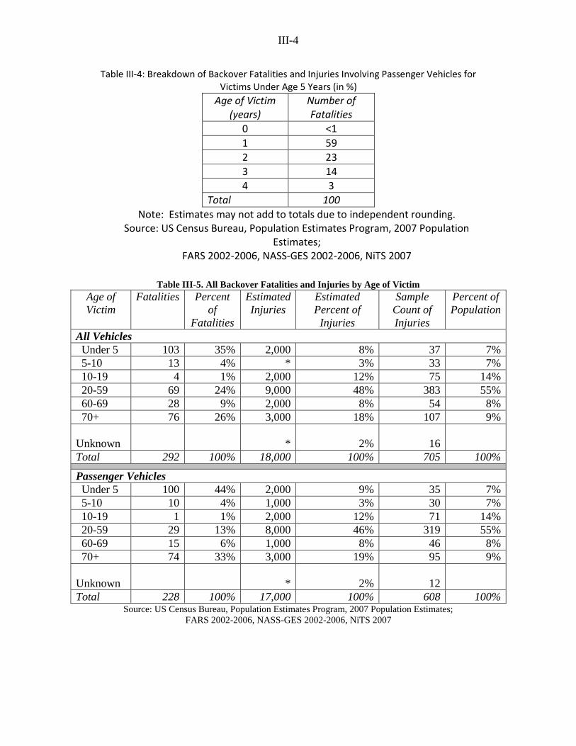
Table III-4: Breakdown of Backover Fatalities and Injuries Involving Passenger Vehicles for Victims Under Age 5 Years (in %)

Age of Victim (years)

Number of Fatalities

0 <1

1 59

2 23

3 14

4 3

Total 100

Note: Estimates may not add to totals due to independent rounding. Source: US Census Bureau, Population Estimates Program, 2007 Population

Estimates; FARS 2002-2006, NASS-GES 2002-2006, NiTS 2007

Table III-5. All Backover Fatalities and Injuries by Age of Victim

Age of

Victim

Fatalities Percent

of

Fatalities

Estimated

Injuries

Estimated

Percent of

Injuries

Sample

Count of

Injuries

Percent of

Population

All Vehicles

Under 5 103 35% 2,000 8% 37 7%

5-10 13 4% * 3% 33 7%

10-19 4 1% 2,000 12% 75 14%

20-59 69 24% 9,000 48% 383 55%

60-69 28 9% 2,000 8% 54 8%

70+ 76 26% 3,000 18% 107 9%

Unknown * 2% 16

Total 292 100% 18,000 100% 705 100%

Passenger Vehicles

Under 5 100 44% 2,000 9% 35 7%

5-10 10 4% 1,000 3% 30 7%

10-19 1 1% 2,000 12% 71 14%

20-59 29 13% 8,000 46% 319 55%

60-69 15 6% 1,000 8% 46 8%

70+ 74 33% 3,000 19% 95 9%

Unknown * 2% 12

Total 228 100% 17,000 100% 608 100% Source: US Census Bureau, Population Estimates Program, 2007 Population Estimates;

FARS 2002-2006, NASS-GES 2002-2006, NiTS 2007

IV-1

IV. Rear Visibility Data While the agency has not determined specific alternatives, one possibility for compliance

testing (as is done in FMVSS No. 111 right now) would be for the agency to develop a

test grid that includes an object that must be directly visible or indirectly visible with

whatever countermeasure is developed by a manufacturer. Tests of current vehicles have

been performed to provide information using a generic test grid. In essence this could be

a performance test, such that when a driver in a vehicle could see a test grid of objects

either through direct visibility by the driver, or through a countermeasure.

Rear Visibility of Current Vehicles

NHTSA found that the area around a vehicle that a driver can directly see without the aid

of non-required mirrors or other devices (i.e., direct –view rear visibility) can be affected

by the exterior, structural design of the vehicle.20

These structural elements included the

width of a vehicle‟s structural pillars and the size of its window openings. Additionally,

vehicles with greater height and length are likely to have larger blind zone areas than

vehicles with smaller dimensions. NHTSA has also found that head restraints can affect

the direct rear visibility.

In 2007, NHTSA observed the rear visibility characteristics of 44 recent-model light

vehicles21

to assess the range of visible areas in the current fleet and provide information

that can be used to determine whether a link exists between the rear blind zone area and

the risk of a backover crash incidence. The visibility of a visual target was determined

over a 6300-square-foot area stretching 35 feet to either side of the vehicle‟s centerline

and 90 feet back from the vehicle‟s rear bumper. The agency selected a 29.4-inch-tall

(approximately the height of a 1-year-old child) visual target. Rear visibility was

measured for both a 50th

percentile adult male driver (69.1 inches tall) and a 5th

percentile

adult female driver (59.8 inches tall). The areas, over which the visual target was

visually discernible using direct glances (i.e., looking out vehicle windows) and indirect

glances (i.e., looking into side or center rearview mirrors), were determined.

Since all passenger vehicles have side mirrors and center rearview mirrors that are

essentially the same (excluding slight overall size differences), NHTSA determined that a

key source of variability affecting rear visibility is a vehicle‟s body structure and interior

components (e.g., rear head restraints). As such, the direct-view rear visibility metric

focused on the impact of a vehicle‟s structural characteristics on rear visibility.

Through this study, NHTSA observed that rear blind zones for individual vehicles ranged

in value from 100 to 1,440 square feet. When summarized by vehicle category and curb

weight (as a surrogate indicator for vehicle size), as illustrated in Figure 1, the data shows

that average direct-view rear blind zone areas varied within these groups. The greatest

range of direct-view rear blind zone area size was seen for the 4,000-5,000 lb SUV group.

Figure 2 illustrates that SUVs (as a whole) were associated with the largest average

20

Light Vehicle Rear Visibility Assessment, DOT HS 810 909, September 2008. 21

Measured vehicles included the ten top-selling passenger cars and light trucks for calendar year 2006.

IV-2

direct-view rear blind zone area as well as the largest range of values for the four body

types examined. Overall, light trucks (segregated here into vans, pickups, and SUVs) as

a vehicle class were observed to have larger rear blind zone areas than passenger cars, as

indicated in Figure 2. While small light pickup trucks had relatively small direct-view

rear blind zone areas, light trucks were generally overrepresented in backover incidents.

Figure IV-1. Direct-View Rear Blind Zone Area by Vehicle Category for a

Measurement Field of 50-Foot Long by 60-Foot Wide. Source: Light Vehicle Rear Visibility Assessment, DOT HS 810 909.

Note: Error bars show the range of values for each vehicle category.

0

100

200

300

400

500

600

700

800

900

1000

1100

1200

1300

1400

PC Light

(2,000-

2,499 lbs)

(N=1)

PC Compact

(2,500-

2,999 lbs)

(N=3)

PC Medium

(3,000-

3,499 lbs)

(N=8)

PC Heavy

(3,500 lbs

and over)

(N=4)

Pickups

<4,000 lbs

(N=3)

Pickups

>4,000 lbs

(N=4)

SUV <4,000

lbs (N=4)

SUV 4,000-

5,000 lbs

(N=5)

SUV 5,000-

6,000 lbs

(N=4)

SUV >6000

lbs (N=1)

Van <5,000

lbs (N=6)

Van

>=5,000 lbs)

(N=1)

Vehicle Category

Av

era

ge

Re

ar

Blin

d Z

on

e A

rea

(S

q. F

t.)

IV-3

Figure IV-2. Direct-View Rear Blind Zone Area by Vehicle Category for a

Measurement Field of 50-Foot Long by 60-Foot Wide. Source: Light Vehicle Rear Visibility Assessment, DOT HS 810 909.

Note: Error bars show the range of values for each vehicle category.

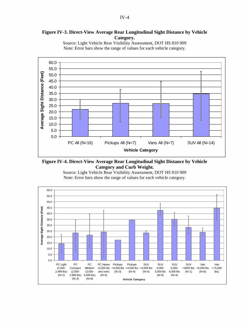
Average direct-view rear longitudinal sight distances were acquired by mathematically

averaging eight longitudinal sight distance measurements taken in 1-foot increments

across the rear of each vehicle. As illustrated in Figure 3, generally light trucks had

longer rear longitudinal sight distances than passenger cars. Exceptions to this trend

included a few small pickup trucks for which average direct-view rear sight distance

values were in the vicinity of those measured for smaller passenger cars, as shown in

Figure 4. Average direct-view rear sight distance values were longest for a full-size van,

SUVs and pickup trucks with a curb weight of 4,000 lbs or greater. Overall, our rear

visibility measurements revealed that light trucks exhibited poor rear visibility when

compared with passenger cars.

0

100

200

300

400

500

600

700

800

900

1000

1100

1200

1300

1400

PC All (N=16) Pickups All (N=7) Vans All (N=7) SUVs All (N=14)

Vehicle Category

Av

era

ge

Re

ar

Blin

d Z

on

e A

rea

(S

q. F

t.)

IV-4

Figure IV-3. Direct-View Average Rear Longitudinal Sight Distance by Vehicle

Category. Source: Light Vehicle Rear Visibility Assessment, DOT HS 810 909

Note: Error bars show the range of values for each vehicle category.

Figure IV-4. Direct-View Average Rear Longitudinal Sight Distance by Vehicle

Category and Curb Weight. Source: Light Vehicle Rear Visibility Assessment, DOT HS 810 909

Note: Error bars show the range of values for each vehicle category.

0.0

5.0

10.0

15.0

20.0

25.0

30.0

35.0

40.0

45.0

50.0

55.0

60.0

PC All (N=16) Pickups All (N=7) Vans All (N=7) SUV All (N=14)

Vehicle Category

Avera

ge S

igh

t D

ista

nce (

Feet)

0.0

5.0

10.0

15.0

20.0

25.0

30.0

35.0

40.0

45.0

50.0

55.0

60.0

PC Light

(2,000-

2,499 lbs)

(N=1)

PC

Compact

(2,500-

2,999 lbs)

(N=3)

PC

Medium

(3,000-

3,499 lbs)

(N=8)

PC Heavy

(3,500 lbs

and over)

(N=4)

Pickups

<4,000 lbs

(N=3)

Pickups

>4,000 lbs

(N=4)

SUV

<4,000 lbs

(N=4)

SUV

4,000-

5,000 lbs

(N=5)

SUV

5,000-

6,000 lbs

(N=4)

SUV

>6000 lbs

(N=1)

Van

<5,000 lbs

(N=6)

Van

>=5,000

lbs)

Vehicle Category

Avera

ge S

igh

t D

ista

nce (

Feet)

IV-5

Relationship Between Rear Visibility and Backing/Backover Crashes Using the rear visibility measurements discussed in the prior section, NHTSA

investigated whether a statistical relationship could be identified between rear visibility

and backing crashes and between rear visibility and backover crashes. For clarification, a

backover is a specifically-defined type of incident, in which a non-occupant of a vehicle

(i.e., a pedestrian or cyclist) is struck by a vehicle moving in reverse. Backing crashes

include the set of all backover crashes, and involve all crashes when the vehicle is

moving in reverse. The implication is if one solves the set of all backing crashes, that

means they have solved the subset of backing crashes that are backovers. Rear visibility

data were used to compute rear visibility metrics which could have a statistical

relationship with backing and/or backover crashes. NHTSA assessed the relationship

between real world backing/backover crashes and rear visibility based on three metrics:

average rear longitudinal sight distance, direct-view rear visibility measurements for a 50

feet long by 60 feet wide test area, and direct-view rear visibility for a 50 feet long by 20

feet wide test area.22

Backing risk was estimated from police-reported crashes in the State Data System.

Backing rates were calculated for 21 vehicle groups with vehicles that had at least 25

backing crashes to account for statistical variability. Backing rate data were provided by

the following states for the specified calendar years:

Alabama (2000-2003) Florida (2000-2005)

Georgia (2000-2005) Illinois (2000-2005)

Kansas (2001-2006) Kentucky (2000-2005)

Maryland (2000-2005) Michigan (2004-2006)

Missouri (2000-2005) Nebraska (2000-2004)

New Mexico (2001-2006) New York (2000)

North Carolina (2000-2005) Pennsylvania (2000-2001, 2003-2005)

Utah (2000-2004) Washington (2002-2005)

Wisconsin (2000-2005) Wyoming (2000-2005)

Simple correlation analysis revealed an association between the two direct-view rear

blind zone areas and backing crash risk. Specifically, larger blind zone areas generally

posed a greater risk of being involved in a backing crash. A statistically significant

relationship23

between backing crash risk and direct-view rear blind zone area was

discovered for both test areas. However, in this analysis, an association between average

rear longitudinal sight distance and backing risk was found to be weaker and not

statistically significant.24

22

Light Vehicle Rear Visibility Assessment, DOT HS 810 909, September 2008 and an unpublished report

by NHTSA‟s Mathematical Analysis Division “Rear Visibility and Backing Risk in Crashes,” December

2008. 23

r=0.51, p=0.02. 24

r=0.26.

IV-6

A multivariate logistic analysis to control for potentially confounding factors produced a

statistically significant25

relationship between backing crash risk and direct-view rear

blind zone area was established for the 50-feet long by 60-feet wide area but not for the

50 feet long by 20 feet wide test area. These calculations suggest that larger blind zone

areas as measured by the wide area are associated with a higher backing crash risk.

Estimated results for the risk of backover crashes using rear longitudinal sight distance

were not statistically significant. Based on the results of the logistic analysis, NHTSA

believes that rear blind zone area measured over a test area 50-feet long by 60-feet wide,

would provide some indication of a vehicle‟s backing crash risk, but may be larger than

needed for a backover rulemaking. This makes some logical sense, since some of the

backing crashes include backing out of a driveway into traffic, and the wider view

available of traffic at speed, the better chance of seeing traffic and not backing into the

street.

In this analysis, the agency examines the costs and benefits of two camera systems - 130

degree and 180 degree cameras. In essence a wider zone would require a 180 degree

camera, rather than a 130 degree camera. While it is enticing to mandate the widest lens

camera and largest display, the SCI data shows that most (85 percent) backovers occur

within a length of 20ft of the starting position, and NHTSA‟s Monte Carlo analysis

suggests a 10 foot wide area. This strongly suggests that a good test requirement for

backover would examine the visibility provided to the driver covering specifically the 10

foot wide by 20 foot long area behind the vehicle. Both the 130 and 180 degree cameras

cover this same space, so either would be appropriate. For perspective, the average blind

zone area for vehicles with no countermeasures extends from the rear of the vehicle, back

over 30 feet.

When examining all backing crashes (including backing into traffic from a driveway), a

wider view of the area behind the vehicle is useful. The length of the view of the

distance directly behind the vehicle is not statistically significantly different between

vehicles. Our theory is that to reduce pedestrian crashes, one needs to see or be able to

sense areas relatively close to the vehicle. For most vehicles we tested, a young child

could not be seen within 12 feet of any of the vehicles, with most having sight distances

beyond 20 feet. We could not find a statistically significant difference in crashes with

vehicles with sight distances 20 to 50 feet back, since most of the need to see is in areas

smaller than that, close to the rear of the vehicle. There were too few vehicles with sight

distance less than 20 feet to determine whether there was a statistically significant

difference between vehicles with a 12 to 20 foot sight distance. Rear visibility data for

over seventy models is available in Appendix B.

For comparison, the following table provides a simplified detection range and the

applicable countermeasures from those examined. It should be noted that the sight

distances in the above tables denote how many feet from the vehicle‟s rear until vision

begins, whereas the numbers below are the distances from the vehicle‟s rear up to the

edge of the vehicle‟s visible range or system detection range. Note that the difference in

25

Chi-square=127, P=<0.001; chi-square=15, P=0.001 respectively.

IV-7

range between 20 feet and 35 feet is not in the camera itself, but in the size of the display

to allow image clarity.

Table IV-1 – Technologies Evaluated, with their Coverage Range

Coverage Range

Technologies that Could Meet this Range

6 ft range Rear-mounted convex mirror, ultrasonic or radar sensors, rearview video system with in-rearview-mirror or in-dash display

16 ft range Radar sensor(s), rearview video system with in-rearview-mirror or in-dash display

20 ft range Rearview video system with in-rearview-mirror or in-dash display

35 ft range Rearview video system with in-dash display

V-1

V. Benefits

A. Probability of a fatal backover being avoided

SCI Case Report Review Background

While a current annual estimate of backover crash fatalities and injuries can be pieced

together from databases such as NiTS, FARS, and NASS-GES, the effectiveness of these

backover methods needs to be created from a source with much more detailed

information. In order to closely examine backover cases, Special Crash Investigations

(SCI) were initiated. By collecting and analyzing a set of in-depth SCI cases, an

estimate of the portion of backover crashes that are avoidable can be made. Test data

from a study about backing aid usage, provides an estimate how many of those avoidable

cases could be avoided. In short the fatalities calculation uses four parts; the target

population of fatalities, F, the percentage of cases found to be “avoidable,” avoidability

(factor fA), the percentage of cases in which the system performs and provides the needed

information (factor fS), and the percentage of cases where drivers will recognize the

information from the system and act appropriately to actually avoid a crash (factor fDR),

and calculate ( F * fA * fS* fDR ), to estimate the potential benefits of different backover

crash countermeasures. Injuries will be calculated similarly.

In order to better understand how avoidable these situations are, a few NHTSA analysts

reviewed 50 available SCI case reports. The Special Crash Investigations are a collection

of in-depth reports made soon after a crash and are not nationally representative, but they

were chosen due to their detail and immediate availability. These are also cases where

investigators had a chance to record volunteered reports and testimonies from police and

those involved in the crash. A team of NHTSA analysts read the case reports, and based

upon that information, decided whether or not the victim was moving at the time of the

backing maneuver, if the victim was detectable given vision, mirrors, cameras, or sensor

systems, and created an estimated, qualitative view of how avoidable the crash was with

the given technologies. Some of the decisions from the team conflict with the coding

from the SCI report, but these differences are mainly regarding whether or not the victim

was moving, and are a product of the team trying to deduce the situation regarding the

crash, rather than to code with certainty what precisely happened.

Pedestrian movement

Before making judgments regarding the ability of the sensors and driver, one single

determination was made that wound up pinning down the nature of the pedestrian case;

was the pedestrian moving? Due to the nature of the SCI investigations, an exact location

for the pedestrians was not available, but many times a description of what the pedestrian

was doing before or during the backing maneuver was available. While determining

pedestrian movement, the team formed one or more sets of scenarios for how the crash

occurred, because precise locations for person and vehicle were not available. Thus,

instead of the single presentation of a court-room style simulation, the team would

sometimes consider multiple such re-enactments per case depending upon the inherent

V-2

ambiguity of the SCI reports. If a pedestrian was moving during the crash, this has a

negative impact on the sensor systems. Examples of phrases within the report that hinted

whether the pedestrian was moving include “riding a bike” and “sitting and playing.”

Also, “moving” is slightly a misnomer as it is a term used to specifically denote a case in

which the pedestrian was not stationary at the beginning of the backing maneuver.

Driver visibility through line-of-sight

The driver‟s visibility is the key to these cases, and despite the results of these cases, a

determination was made based on the supposed pedestrian location (as determined by the

narrative made by the SCI case author), and the visibility profile of the vehicle as laid out

in the blind spot diagrams in the report. The two types of visibility catalogued in the

evaluation were direct vision and visibility using mirrors. A pedestrian was visible using

direct vision if they were visible by direct line-of-sight (no mirrors) to an average driver

in the driver‟s seat. This visual data is expected to be collected starting ten seconds prior

to and throughout the backing motion. Thus, the pedestrian was “directly visible” if the

driver would have seen them within or entering the upcoming backing trajectory of the

vehicle, even before the vehicle was put into its rearward motion. This definition

eliminates cases where a person is known to be within the vicinity of the vehicle, but the

driver does not have recent or current line-of-sight to that person. With regard to

“meaningful” amounts of data, the analysts attempted to assess the cases so that a “split

second” view or obstructed view would not be coded as “visible,” as it would be too

difficult to ascertain visually that there was a pedestrian in the way, nor would cases with

insufficient reaction time given the circumstances be coded as “visible.” “Visible using

mirrors” refers to the same constraints, excepting of course that the pedestrian had to be

visible within the mirrors (any of the side and center rear view mirrors) rather than by

direct line-of-sight.

Ability to Detect Pedestrians

A large part in the determination of whether a certain case could have been avoided was

to determine in every case if the situation was one that could have been averted with the

aid of certain technologies; in a word, whether the pedestrian was “detectable.” This is

completely separate from the human factor of what the particular driver in the case was

doing, as well as what an ideal driver would have been able to do. Simply put, would the

countermeasure in question show or display any sign of the pedestrian whatsoever,

regardless of how much time was left to the driver? After determining whether the

technology would have detected the pedestrian, the next step is to ascertain if a prudent

driver (as opposed to the driver of the case vehicle) would have been able to use such a

technology in order to avoid the crash.

The driver‟s ability to perceive objects behind the vehicle can be aided by various sensor

technologies. The two considered were ultrasonic and radar systems, which can sense 1

year old children within these detection zones below as in Figure 5. These systems,

especially ultrasonics, are known to be unreliable at picking up small objects, such as

children, and have difficulty picking up objects that pass into the detection zone laterally.

Stationary pedestrians that are larger in size or are as high as the bumper have an

V-3

increased chance of being detected reliably. Sensor systems were assumed to cutoff

above 3 mph. Radar systems perform better than ultrasonic systems in detecting distance

to and recognition of people. Infra-red systems and composite systems used to

differentiate human beings from their environment are available or theoretically possible,

but were not considered in these case reviews.

*Figure V-1 – Ultrasonic and Radar Sensor Detection Area*

V-4

Camera systems were also evaluated by the team. The display is assumed to be active

immediately (a fraction of a second at most) after the vehicle is engaged in reverse

(therefore, before and during the backing motion). However, the expectation is that a

conscientious driver will look in the display before backing up, just as a conscientious

driver is told to look behind them using mirrors or over their shoulder. Cameras have a

single cone of visibility, and as such will not be able to see directly beneath the bumper,

depending on practical placement and vehicle design. It was assumed that the camera

would be placed aiming downward, and above the license plate, rendering it useless if a

rear hatch (or other license fixture) was raised, or if the pedestrian was already fully

underneath the car. Both 180 degree and 130 degree camera models were used in the

evaluation. The 130 degree cameras were assumed to have slightly less ability at picking

up pedestrians entering the viewing area laterally than the 180 degree camera. A good

indication that a pedestrian was visible to the camera was if the report stated the

pedestrian moved from one side of the vehicle and was struck by the rear of the vehicle

on the other side. This does not necessarily mean that the crash was avoidable, merely

that the pedestrian was visible (the wide angle of view assures that even a pedestrian

running laterally towards the rear of the vehicle would be seen for a significant amount of

time, barring viewing obstructions) Generally, if the pedestrian hit the center of the

bumper it was assumed that the crash was visible from either type of camera. Figure 6

below shows the field of view for the two hypothetical camera systems used by the team.

V-5

Figure V-2 – Visible display area for camera systems

Crash Avoidability

It was estimated whether or not the pedestrian crash was “avoidable” using each

of the different technologies by assuming a prudent driver is either looking at the

technology and/or reacting to the technology at all of these times:

a) before putting the vehicle in reverse

b) after shifting into reverse, but before removing pressure to the brake

c) while moving the vehicle in reverse

d) at the time that the pedestrian enters into the space behind the vehicle and is

threatened by its rearward motion.

e) at the time that the vehicle turned to put the pedestrian within a collision course

This means that the driver would not begin backing, or alternatively, stop backing

immediately and fully, if they are given a sensor based warning or a camera based visual

identification of a hazard. The goal of the analysts reading the SCI Reports was to

establish an “avoidability” criterion, and this was done through a series of judgments

regarding the crash situation. For example, was the victim moving? Was the victim

visible using direct vision, mirrors, or cameras? Was the victim detectible using sensor

systems? These questions were answered with yes, no, or unknown. All of these factors

contributed to the final answers for the four final columns in Table 1 below, the

V-6

avoidability for given technologies. However, there is no algorithm that translates from a

case‟s disparate elements to its likelihood to be avoided. The possibility of avoidance

was defined with the following statement: “Given your understanding of the

circumstances presented in the case, would a prudent driver properly utilizing their

vehicle and the backing technology in question be very likely, likely, unlikely, or very

unlikely to avoid the pedestrian? Answer Yes, Probably Yes, Probably No, No

respectively, or “unknown” if not enough information was available to make a judgment

on the case. Cases in which there was a relative lack of knowledge, and cases which

evoked weaker, less confident answers were marked as “probably.” If the pedestrian was

not “detectable” as determined earlier, no information gets passed onto the driver, which

means the driver then has no reason to halt the backing maneuver. Below is by no means

a comprehensive list of reasons for cases not being avoidable, but simply serve as a list of

indicators guiding the reviewers‟ opinions. No single reason is ever given per case to

describe why it was not avoidable, but rather the avoidability criterion is an inseparable

amalgam of multiple factors.

1. Victim moving into path – If a pedestrian enters the path of the backing vehicle

laterally, not giving enough time for the driver to react, that decreases the chance

of avoidance.

2. Vehicle turning while backing – The team assumed that in most cases, when a

vehicle was turning, their camera would continue to capture the majority of the

event as it transpires as the image is captured from a wide-angle source, but

would possibly suffer a small decrease in avoidance capability. As for sensors,

this decrease in avoidance capability was greater, as the sensors would be

sweeping out into a new area behind the vehicle, decreasing the time the

pedestrian was detectable before impact.

3. If the pedestrian was low to the ground or was a small child, but the team decided

it was still “detected” earlier in the case analysis, the avoidability would most

likely be decreased slightly due to the fact that the sensor system would take

longer to detect the pedestrian.

4. Increased relative vehicle speed – Faster vehicle backing speeds and faster

pedestrian movement towards the vehicle both decrease the reaction time

available for all systems.

5. Obfuscation and atmospheric conditions – Poor visibility (trees, shrubberies,

snow, glare, fog, etc.) can impair the driver recognizing the pedestrian within the

display. This was not a factor in most cases.

6. Incline of the road – Backing down a decline decreases the effectiveness of

sensors the further away from the car the pedestrian is.

7. Pedestrian position – If it was difficult to determine where the pedestrian was, if

they moved, or when they moved (in other words, if there were some level of

uncertainty), that would negatively impact the likelihood that the crash could have

been avoided, in order to keep our estimation of system performance a

conservative one. This means that uncertainty regarding pedestrian position and

movement affects both the visibility or detectability and the avoidability.

V-7

It is also worth noting that no effort was taken to account for recklessness, inebriation, or

fatigue. All discussions of cases included a theoretical „perfect‟ driver, and assumed that

the technology was working as intended. No evidence was found within the cases to

identify driver impairment as a significant cause of backover crashes. An estimation of

the human part of the equation will be shown later on, and will be derived from human

factors testing.

SCI Case Report Review Procedure and Results

Cases were reviewed individually, and the group met several times to reach a

consensus that all members were satisfied best explained the situations. If no consensus

could be made by the group, the results were averaged into one response. In the case of

the “Possibility of Avoidance,” the group would consider the scenario, taking into

consideration the factors above and any special factors unique to the case. In one report,

the driver reported that their parking space existed on a hill that required a significant

amount of throttle to be used while backing up. It was then assumed that a reasonable

driver in such a situation would indeed be driving at such an increased speed. Although

there was no strict formula as to how avoidability was determined, a general guideline

was to look at the detection zone, blind spots, and visibility areas. If the pedestrian was

detectable, then what followed was a cataloguing of all the impediments to a reasonable

driver reacting in time after receiving a warning or recognizing a pedestrian on a display.

The most sensitive part of the study was most likely the pedestrian‟s position and actions

during the event. When the team disagreed on nuances of the pedestrian‟s role in the

crash, the possibility of avoidance would most likely be arbitrated to an average value.

The complete results of the evaluation are shown in Table 2.

V-8

Table V-1: Evaluation Team‟s Judgments regarding Movement, Detection, and

Avoidability of 2007 SCI Backover Cases

Victim

moving?

Victim path passed through sensor

detection zone?

(Y/N/Unk)

Possibility of Avoidance

(Y/N/ Victim Visible? Y=Yes

Unk) (Y/N/Unk) PY=Possibly Yes

PN=Possibly NO

N=No Unk = Unknown

Using direct vision

Using mirrors

in 180o

camera view

in 130o

camera view

Ultra-sonic Radar

in 180o

camera view

in 130o

camera view

Ultra-sonic Radar

Y 32 21 27 47 44 45 45 33 25 10 12

PY 12 13 14 15

PN 2 5 10 10

N 10 23 18 3 5 3 3 3 7 15 12

UNK 8 6 5 0 1 2 2 0 0 1 1

Y 64% 42% 54% 94% 88% 90% 90% 66% 50% 20% 24%

PY 24% 26% 28% 30%

PN 4% 10% 20% 20%

N 20% 46% 36% 6% 10% 6% 6% 6% 14% 30% 24%

UNK 16% 12% 10% 0% 2% 4% 4% 0% 0% 2% 2%

(Y) as % of

Known 76% 48% 60% 94% 90% 94% 94% 66% 50% 20% 24% (Y) or (PY) as %

of Known 90% 76% 49% 54%

It should be restated that these results are the product of a team of analysts working to

determine a clear vision of each SCI case, and as such are do not carry the precision

found in the FARS files or even the very SCI cases from which they are gleaned.

However, it represents our best estimate of the possibility of avoidance given the

currently available data. The majority of cases involved moving pedestrians. Of the

known cases, 76 percent (32/42) of the victims were moving. In just under half of the

known cases (21/44), victims were visible using direct vision at some time slightly before

or during the maneuver. However, in at least 90 percent of all known cases (44/48 to

47/50), for all four technologies considered, the pedestrian was at some point in a zone

that was detectable by the sensors or visible by cameras. As for avoidability, 90 percent

of cases were flagged as “yes” or “probably yes” for the 180 degree camera, compared

with 76 percent for 130 degrees. The sensor systems did not fare as well as the camera

systems, as they have a 49 and 54 percent avoidability estimate for ultrasonic and radar

systems, respectively.

Human Factors

NHTSA performed a number of research projects on drivers after they had been driving

for a few months in vehicles with either:

V-9

1) No backup system

2) Camera systems (Rear Video = RV)

3) A Camera system (RV) and a Sensor System (Rear Parking Sensor System = RPS)

One of the aspects of this testing was a staged event, where a cardboard child size object

with a picture of a child on it popped up from the ground directly behind the vehicle as

they were backing up in a spot where they would have no notion or idea that a child could

be anywhere in the vicinity. At that time, cameras recorded their head and eye

movements to see how they backed up, whether they looked at the mirrors or video

displays from the camera, whether they paid attention to warnings provided by the rear

parking sensor system, and other related information.

Table 3 shows the results of that staged event. All of the drivers with no backup system

hit the cardboard child, 58 percent with a camera system only hit the cardboard child and

85 percent of those with a camera and rear parking sensor system hit the cardboard child.

The results of the staged event might be considered somewhat counter-intuitive – the

camera systems (RV) and rear parking sensor systems Sensor Systems (RPS) together

were less effective than just a camera system, although this distinction was not

statistically significant. From that same report, driver glances at the camera display were

fewer when the vehicle was equipped with both systems – however, it should be noted

that the sensor was located in the instrument panel, not integrated with or near the camera

display. Also, the camera in this study had a long delay (6 seconds) before turning on,

but this delay was ignored within the constraints of the SCI case review.

In the PRIA accompanying the ANPRM, we made the following statements relating to

the effectiveness of camera systems and driver response. These data and later collected

data have been combined into Table V-3.

V-10

Table V-2: Staged Obstacle Event Outcomes26

System N Number that Crashed Percent Crashed

No system 12 12 100%

RV only 12 7 58%

RV & RPS 13 11 85%

Total 37 30 81%

In that same event, 15 of the 25 drivers glanced at their mirrors at least once during the

event, and 9 of those 15 looked multiple times. This data represents the human factor.

Thus, it is assumed that 9/15 = 60 percent of cases involve drivers that are the

hypothetical prudent drivers that are constantly aware while backing up, using the

camera. All 7 of the drivers that avoided hitting the cardboard child looked multiple

times. In the end, the number that counts is (5+2)/25 = 28 percent of cases with both RV

only and RV & RPS in which the driver avoided the staged obstacle event. Since both

systems had cameras, it was appropriate to try to estimate different effectiveness

estimates for different countermeasures from this data. This represents the percentage of

times that a driver will correctly respond in an avoidable situation.

This is a small experiment with 25 drivers. While it is likely that the camera‟s

effectiveness estimate is somewhere in the area around 28 percent, there is uncertainty

around that estimate and a reasonable range of effectiveness might be 15 to 40 percent.

In a similar fashion, we must estimate likely driver reaction to sensors. The ORSDURVS

report provides a machine detection factor of 39 percent for the sensors (an ultrasonic

system was used). This is an additional factor that must be considered when calculating

benefits, as the system and the human driver need to both correctly respond to the

pedestrian. After the system provides a warning, regardless of the driver‟s glance pattern

their attention would be drawn to the threat of collision, providing an estimated 15

percent improvement in driver reaction over the camera system. Thus, it is likely that the

effectiveness estimate is somewhere in the area around 43 percent, and a reasonable

range of effectiveness might be 30 to 55 percent. Again, this was the logic presented in

the February 2009 PRIA accompanying the ANPRM. For this PRIA, we combined the

RV data with more recent testing, but decided against combining the RV & RPS system

data with the RV only data (see Table V-3).

Human Factors 2009 Update

In 2009, VRTC performed additional testing with various backover avoidance

technologies. This was done to improve the available knowledge of driver behavior. The

new data was added to the previous set of Staged Obstacle Event Outcomes, and a

combined table of both data sets follows.

26

Table 6 from On-Road Study of Drivers‟ Use of Rearview Video Systems (ORSDURVS) – Elizabeth

Mazzae

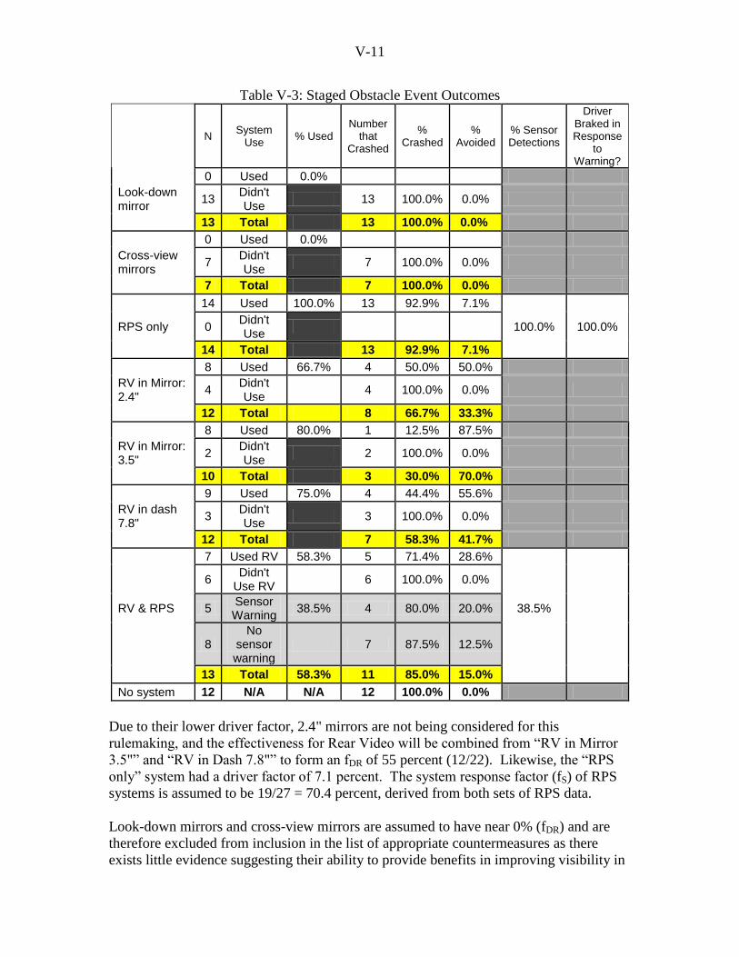
V-11

Table V-3: Staged Obstacle Event Outcomes

N System

Use % Used

Number that

Crashed

% Crashed

% Avoided

% Sensor Detections

Driver Braked in Response

to Warning?

0 Used 0.0%

Look-down mirror

13 Didn't Use

13 100.0% 0.0%

13 Total 13 100.0% 0.0%

0 Used 0.0%

Cross-view mirrors

7 Didn't Use

7 100.0% 0.0%

7 Total 7 100.0% 0.0%

14 Used 100.0% 13 92.9% 7.1%

RPS only 0 Didn't Use

100.0% 100.0%

14 Total 13 92.9% 7.1%

8 Used 66.7% 4 50.0% 50.0%

RV in Mirror: 2.4"

4 Didn't Use

4 100.0% 0.0%

12 Total 8 66.7% 33.3%

8 Used 80.0% 1 12.5% 87.5%

RV in Mirror: 3.5"

2 Didn't Use

2 100.0% 0.0%

10 Total 3 30.0% 70.0%

9 Used 75.0% 4 44.4% 55.6%

RV in dash 7.8"

3 Didn't Use

3 100.0% 0.0%

12 Total 7 58.3% 41.7%

7 Used RV 58.3% 5 71.4% 28.6%

6 Didn't

Use RV 6 100.0% 0.0%

RV & RPS 5 Sensor Warning

38.5% 4 80.0% 20.0% 38.5%

8 No

sensor warning

7 87.5% 12.5%

13 Total 58.3% 11 85.0% 15.0%

No system 12 N/A N/A 12 100.0% 0.0%

Due to their lower driver factor, 2.4" mirrors are not being considered for this

rulemaking, and the effectiveness for Rear Video will be combined from “RV in Mirror

3.5"” and “RV in Dash 7.8"” to form an fDR of 55 percent (12/22). Likewise, the “RPS

only” system had a driver factor of 7.1 percent. The system response factor (fS) of RPS

systems is assumed to be 19/27 = 70.4 percent, derived from both sets of RPS data.

Look-down mirrors and cross-view mirrors are assumed to have near 0% (fDR) and are

therefore excluded from inclusion in the list of appropriate countermeasures as there

exists little evidence suggesting their ability to provide benefits in improving visibility in

V-12

certain areas behind the vehicle. Some evidence exists to show that cross-view mirrors

may produce a 33.4% potential backover crash reduction if a driver looks at a mirror once

prior to the start of a backing maneuver.27

Achieving this potential reduction is

dependent upon drivers actually using the mirrors, but the above research summarized in

Table 4 shows that even drivers familiar with the mirrors failed to use them.

It is worthwhile to mention that in all cases where the “RPS only” system provided an

alert, all drivers reacted in some way, and no drivers were able to avoid a collision. The

RPS systems used in these cases were both ultrasonic systems, and due to no similar

available data regarding radar systems, the fDR and fS for radar systems will be assumed to

be equal to that of ultrasonic systems, while the SCI case review accounted for the

increased range of the radar, reflected in a higher fA for radar. In general, drivers that

received a warning from a sensor (RPS), sometimes stopped the vehicle and then looked

out the rear window. When they were unable to visually see an obstruction, they

continued on and ran over the cardboard child figure. Participants‟ comments following

the conflict scenario were collected, confirming this progression of events. We assume

that this same driver reaction would have taken place regardless of whether the sensor

was ultrasonic or radar. That is to say that most drivers tend not to fully believe the

information provided by sensor systems.

Before proceeding into the calculation of benefits, one final note must be made. In all 20

cases, using either cross-view mirrors or look-down mirrors, the driver failed to avoid the

test object. The human factors testing provides our only information regarding the

driver‟s willingness to use the technology available to them. While, as mentioned earlier

in Chapter II, other sources may claim that “when drivers use them, mirrors provide

benefits,” there is no indication that even drivers familiar with the systems will decide to

use them. Finally, by concluding that fDR is 0% for mirrors, the overall effectiveness

given by (fA * fS* fDR ) must also equal 0%. In other words, no matter how many

backover cases are avoidable (fA) using mirrors, and despite even an assumption that the

system (fS) performs perfectly 100% of the time, if nobody‟s looking carefully at the

mirror while performing a backing maneuver, the system provides no benefits. For this

reason only, analysis of mirrors has been set aside for the remainder of the document. If

evidence of increased driver acceptance of this system is provided, mirrors will be

reintroduced to the benefits discussion, but as of right now, there is no evidence that they

will provide any benefits at all.

B. Benefits Calculations

Previous sections established the backover fatalities, F, which are comprised of an

estimated 228 light vehicles, (59 passenger cars, 68 sport utility vehicles, 29 vans, and 72

pickups). Applied next is the 55 percent estimate for successful driver reaction with

cameras and the 7 percent estimate for sensors, as fDR. Sensors also apply the 70 percent

detection rating for fS whereas Cameras are assumed to have fS = 100 percent. Finally,

27

Garrot, “The Ability of Rear-mounted Convex Mirrors to Improve Rear Visibility” http://www-

nrd.nhtsa.dot.gov/pdf/esv/esv21/09-0558.pdf

V-13

for the various systems, the avoidability percentages from the SCI case investigations are

used, selecting the cases marked “Yes” or “Possibly Yes” from the total number of cases.

Table V-4: Avoidability and Potential Lives Saved by Technology after Successful

Driver Reaction

Successful

Driver

Camera

Reaction

(fDR)

in 180o

camera view

in 130o

camera view

Ultra-sonic

Radar Sensor

Picks Up

Pedestrian

(Detection

Rating)

Successful

Driver

Sensor

Reaction

(fDR)

Avoidable (Y) 66% 50% 20% 24%

Avoidable (Y, PY) 90% 76% 49% 54%

55% Avoided (Y) 36% 27% 1% 1% 70% 7%

Avoided (Y, PY) 49% 41% 1% 2%

55% Lives Saved (Y) 82 62 1 2 70% 7%

Lives Saved (Y, PY) 112 95 3 3

In the lower portion of the above table, ( F * fA * fS * fDR ), has been calculated to

estimate the potential benefits of the different backover crash countermeasures. Below,

these numbers have been further broken down by using the same factors, but examining

the distribution of passenger cars and light trucks found in the fatality target population.

V-14

Table V-5: Estimated Lives Saved by Vehicle Type 55% for camera

OR 7%*for sensor

180o camera 130

o camera Ultrasonic Radar

Pass Car (Y) 21 16 0 0

LT (Y) 61 46 1 1

Total (Y) 82 62 1 2

Pass Car (Y,PY) 29 25 1 1

LT (Y,PY) 83 70 2 3

Total (Y,PY) 112 95 3 3

Table 6: Estimated Injuries Avoided by Vehicle Type 55% for camera

OR 7%*for sensor

180o camera 130

o camera Ultrasonic Radar

Pass Car (Y) 3,29028

2,492 51 61

LT (Y) 2,852 2,160 44 53

Total (Y) 6,141 4,652 95 114

Pass Car (Y,PY) 4,486 3,788 125 137

LT (Y,PY) 3,888 3,284 108 119

Total (Y,PY) 8,374 7,072 233 257

*55% refers to successful driver reaction for cameras, 7% refers to successful driver

reaction to ultrasonic or radar sensors. Note, some numbers are off by one, due to

rounding

Thus, the total number of lives saved from camera systems could be between 62 and 112,

and from sensor systems between 1 and 3. We assume the same effectiveness for injury

cases as we do for fatalities. Injury reduction would be between 4,652 and 8,374 for

cameras and between 95 and 257 for sensors.

C. Property Damage Only Crashes and Maintenance Costs

In a Preliminary Cost-Benefit Analysis of Ultrasonic and Camera Backup Systems29

,

NHTSA modeled benefits and costs (excluding injuries and fatality benefits) from a

societal perspective to determine cost effectiveness of such systems with regard to only

installation, and maintenance and repair costs, and the benefits derived from backing

avoidance. This model establishes that although benefits are generated when the driver

successfully avoids a crash, unexpected costs arise when the system is damaged or

destroyed in non-backing crashes, namely struck-from-the-rear collisions.

The findings of that analysis were that for a range of crash distributions (10 to 25 percent

of rear-damaged vehicles were backing, as opposed to 75 to 90 percent of rear-damages

vehicles were struck-from-the-rear), and for a range of driver factors (50% to 80%

successful driver reaction), none of the systems were nearly cost-effective. Overall, the

net costs with the old figures ranged from $45 to $468 per vehicle.

28

Calculated for example: 9138 Injuries * 54.54% driver factor * 66% camera avoidance factor 29

See NHTSA docket 2006-25579-2.

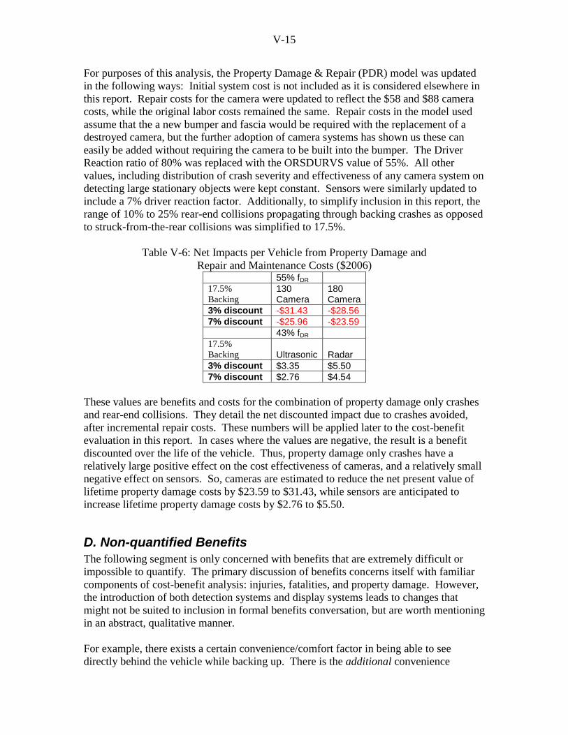
V-15

For purposes of this analysis, the Property Damage & Repair (PDR) model was updated

in the following ways: Initial system cost is not included as it is considered elsewhere in

this report. Repair costs for the camera were updated to reflect the $58 and $88 camera

costs, while the original labor costs remained the same. Repair costs in the model used

assume that the a new bumper and fascia would be required with the replacement of a

destroyed camera, but the further adoption of camera systems has shown us these can

easily be added without requiring the camera to be built into the bumper. The Driver

Reaction ratio of 80% was replaced with the ORSDURVS value of 55%. All other

values, including distribution of crash severity and effectiveness of any camera system on

detecting large stationary objects were kept constant. Sensors were similarly updated to

include a 7% driver reaction factor. Additionally, to simplify inclusion in this report, the

range of 10% to 25% rear-end collisions propagating through backing crashes as opposed

to struck-from-the-rear collisions was simplified to 17.5%.

Table V-6: Net Impacts per Vehicle from Property Damage and

Repair and Maintenance Costs ($2006) 55% fDR

17.5%

Backing 130 Camera

180 Camera

3% discount -$31.43 -$28.56

7% discount -$25.96 -$23.59

43% fDR

17.5%

Backing Ultrasonic Radar

3% discount $3.35 $5.50

7% discount $2.76 $4.54

These values are benefits and costs for the combination of property damage only crashes

and rear-end collisions. They detail the net discounted impact due to crashes avoided,

after incremental repair costs. These numbers will be applied later to the cost-benefit

evaluation in this report. In cases where the values are negative, the result is a benefit

discounted over the life of the vehicle. Thus, property damage only crashes have a

relatively large positive effect on the cost effectiveness of cameras, and a relatively small

negative effect on sensors. So, cameras are estimated to reduce the net present value of

lifetime property damage costs by $23.59 to $31.43, while sensors are anticipated to

increase lifetime property damage costs by $2.76 to $5.50.

D. Non-quantified Benefits

The following segment is only concerned with benefits that are extremely difficult or

impossible to quantify. The primary discussion of benefits concerns itself with familiar

components of cost-benefit analysis: injuries, fatalities, and property damage. However,

the introduction of both detection systems and display systems leads to changes that

might not be suited to inclusion in formal benefits conversation, but are worth mentioning

in an abstract, qualitative manner.

For example, there exists a certain convenience/comfort factor in being able to see

directly behind the vehicle while backing up. There is the additional convenience

V-16

distinct from and beyond the potential fatalities, injuries, and property damage. This

convenience/comfort factor is a reduction in anxiety or apprehension while backing up.

Similarly, the improved ability to parallel park (whose property damage benefits are

already discussed) may provide a decreased delay in traffic while a driver cautiously

parallel parks in one attempt rather than in multiple attempts.

If a display is used in the dash, other information could be provided, not only navigation,

but potentially safety warnings. It seems that the first rulemaking to introduce a display

suffers the installation cost, and subsequent rulemakings piggyback on the mandated

display to provide context-sensitive safety benefits. The display for a camera system has

the additional “benefit” of facilitating the introduction of other safety systems. The

incremental cost of installing those “other” systems will not take into account the cost of

the display, because they were already accounted for via the rear visibility rulemaking.

In this way, the non-quantifiable impact of mandating displays leads to the possibility of

the introduction of other safety mechanisms, or decreased costs in deploying said

mechanisms. All the preceding conversation regarding possible consequences is not

typical of cost-benefit analysis, is completely qualitative, and merely should be taken as a

simple reminder. The display unit in question will doubtless have purposes other than to

provide a display when the vehicle is in reverse and remain dormant and inactive

otherwise, and any other safety technology to use the display will not include display cost

in its analysis.

The comprehensive cost of an injury/fatality includes time lost on the job, and time lost at

home, but only for the case of the injured. The emotional well-being of the extended

family members, friends, and other associates of the injured is not included in cost-

benefit analysis. Even non-injured drivers in pedestrian crashes are not given injury

costs. Above and beyond the physical injuries sustained by the pedestrian victim, it can

be argued that the emotional distress of the driver should be counted, especially in cases

where the driver injures a child, and even more so when the child is their own. Cost data

for driver distress due to such “perceived guilt” or “shock” is not available for crashes, let

alone for crashes involving family member fatalities. More information would be

required for rigorous inclusion in a formal analysis, but this emotional response is

potentially one of the results of a backover crash, and its personal nature may place more

emotional weight behind it than an accident involving a total stranger to the driver.

The agency requests comments on these non-quantified benefits.

VI-1

VI. Costs The costs for improving rear visibility are found in both the installation and

maintenance/repair of the various parts for a variety of technological options. Systems

are comprised of some sort of sensing apparatus almost exclusively found in the rear of

the vehicle, usually located in the bumper or directly above the license plate. This is

important because some rear-end collisions (when the vehicle is struck in the rear by

another vehicle) will impact the backover avoidance system, possibly requiring

recalibration, repair, or replacement. In the report “Preliminary Cost-Benefit Analysis of

Ultrasonic and Camera Backup Systems” these costs were detailed, based upon a

methodology of “lifetime crashes.” The repair costs for cameras, when combined with

their benefits from avoiding property damage only crashes are evaluated in the previous

section, as they provide a net benefit.

The cost of installing one of these systems varies greatly with the type of system being

installed. Initial vehicle part costs (or manufacturer costs) were multiplied by 1.51 to find

the cost to consumers on a per-vehicle basis. The sensor systems (including a warning

buzzer) are less expensive than a camera system. We estimate the cost of an ultrasonic

system at $51-$89, an infrared system at $47, and a radar system at $92. For camera

systems, the display method is the primary discerning factor; a system with a camera and

a dashboard display may cost up to $189, but a vehicle that‟s already equipped with a

navigational device already has a screen and the total cost comes to $88.18.30

The

incremental cost for installing any system (sensor or camera) is decreased if the sensor‟s

warning or the camera‟s image is routed through an already present display or speaker

system. Thus, if a vehicle is already equipped with an in-dash navigation unit, no extra

display would be required, eliminating the cost of the display. Because estimated prices

for these systems have decreased over time, further comments for the proposed

installation rate, current availability, and cost of these systems will continue to be

welcomed, as are comments regarding alternative systems that would cost less and meet

the proposed statutory requirement.

Each camera system cost was estimated based on a collection of confidential industry

estimates and internal NHTSA estimates for small parts and the assembly process.

Camera prices (for the lens and light sensing apparatus) are estimated to average $30 for

130 degree cameras and $50 for 180 degree cameras. Wiring for dash display systems

was set to $8, but $11 for rear mirror display systems due to the wire navigating the A

pillar and climbing forward to the rear view mirror. Assembly labor was estimated at

$23.69/hr, and applied to a 3 minute installation time for a dash display system and

camera for an assembly cost of $1.20. Alternatively, the 3.5 minute installation time for

a mirror system, including the time to run the wire up the A pillar and around the

windshield, comes to $1.40. Supposing the vehicle was already equipped with a display

unit from a navigation system, the labor to simply install the camera would be 1 minute,

or $0.40. Estimates from various manufacturers and parts suppliers were submitted,

30

All cost numbers for these systems are comprised of confidential data from vehicle manufacturers, data

from dealerships, and data from system manufacturers. Teardown analysis of backover avoidance

technologies is forthcoming as of November 2010.

VI-2

however the costs for these systems seemed inflated to the price of large retail display

units and were therefore brought back to a manufacturer costs by division by a factor of

1.51. From this we estimate mirror displays cost at $73, and dash displays at $66. A

camera system with a rear-view mirror display costs between $173 and $203.

Table VI-1

Estimated Consumer Costs ($2007)

130 Mirror 180 Mirror 130 Dash 180 Dash

Entire Camera System Required $172.74 $202.94 $158.85 $189.05

Nav Unit Present, Cam & Wires needed $57.98 $88.18

Ultrasonic Radar

Sensor System $51.49 $92.26

For the purpose of this analysis, the number of vehicles equipped with cameras needed to

be compiled from a variety of sources. The 2008 Wards Automotive Yearbook provides

detailed sales for certain equipment for all 2007 cars. This, combined with comments

from the industry, led us to assume the following current distribution of cars sold. We

assumed that the distribution of the 22% of light trucks equipped with “rear object

detection” are 5% camera, 18% sensor, and 1% combined systems. We also assumed

that all camera-equipped systems already were equipped with a navigational unit in the

dash.

Table VI-2a

Estimated MY 2007 Backover Systems

Cars need display & Camera 93%

Cars w/ nav, no camera 7%

Cars fully equipped already 0%

Light Trucks need display & Camera* 82%

Light Trucks w/ nav, no camera* 13%

Light Trucks fully equipped already* 5%

*Assumes that the 22% trucks equipped with "rear object detection" are 5% camera, 18% sensor, and 1% overlap

*Assumes that all camera-equipped systems have navigation units in the dash

Regarding sensors, the installation rates were also taken from Wards, using the above

assumption to arrive at 4 percent of passenger cars and 18 percent of light truck vehicles

equipped with some sort of sensor system.

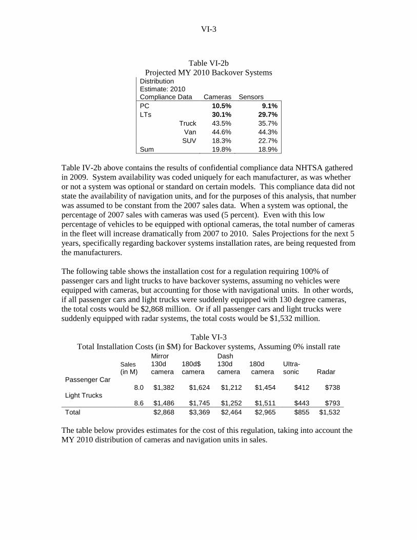
VI-3

Table VI-2b

Projected MY 2010 Backover Systems Distribution Estimate: 2010 Compliance Data Cameras Sensors

PC 10.5% 9.1%

LTs 30.1% 29.7%

Truck 43.5% 35.7%

Van 44.6% 44.3%

SUV 18.3% 22.7%

Sum 19.8% 18.9%

Table IV-2b above contains the results of confidential compliance data NHTSA gathered

in 2009. System availability was coded uniquely for each manufacturer, as was whether

or not a system was optional or standard on certain models. This compliance data did not

state the availability of navigation units, and for the purposes of this analysis, that number

was assumed to be constant from the 2007 sales data. When a system was optional, the

percentage of 2007 sales with cameras was used (5 percent). Even with this low

percentage of vehicles to be equipped with optional cameras, the total number of cameras

in the fleet will increase dramatically from 2007 to 2010. Sales Projections for the next 5

years, specifically regarding backover systems installation rates, are being requested from

the manufacturers.

The following table shows the installation cost for a regulation requiring 100% of

passenger cars and light trucks to have backover systems, assuming no vehicles were

equipped with cameras, but accounting for those with navigational units. In other words,

if all passenger cars and light trucks were suddenly equipped with 130 degree cameras,

the total costs would be $2,868 million. Or if all passenger cars and light trucks were

suddenly equipped with radar systems, the total costs would be $1,532 million.

Table VI-3

Total Installation Costs (in $M) for Backover systems, Assuming 0% install rate Mirror Dash

Sales (in M)

130d camera

180d$ camera

130d camera

180d camera

UItra-sonic Radar

Passenger Car 8.0 $1,382 $1,624 $1,212 $1,454 $412 $738 Light Trucks 8.6 $1,486 $1,745 $1,252 $1,511 $443 $793

Total $2,868 $3,369 $2,464 $2,965 $855 $1,532

The table below provides estimates for the cost of this regulation, taking into account the

MY 2010 distribution of cameras and navigation units in sales.

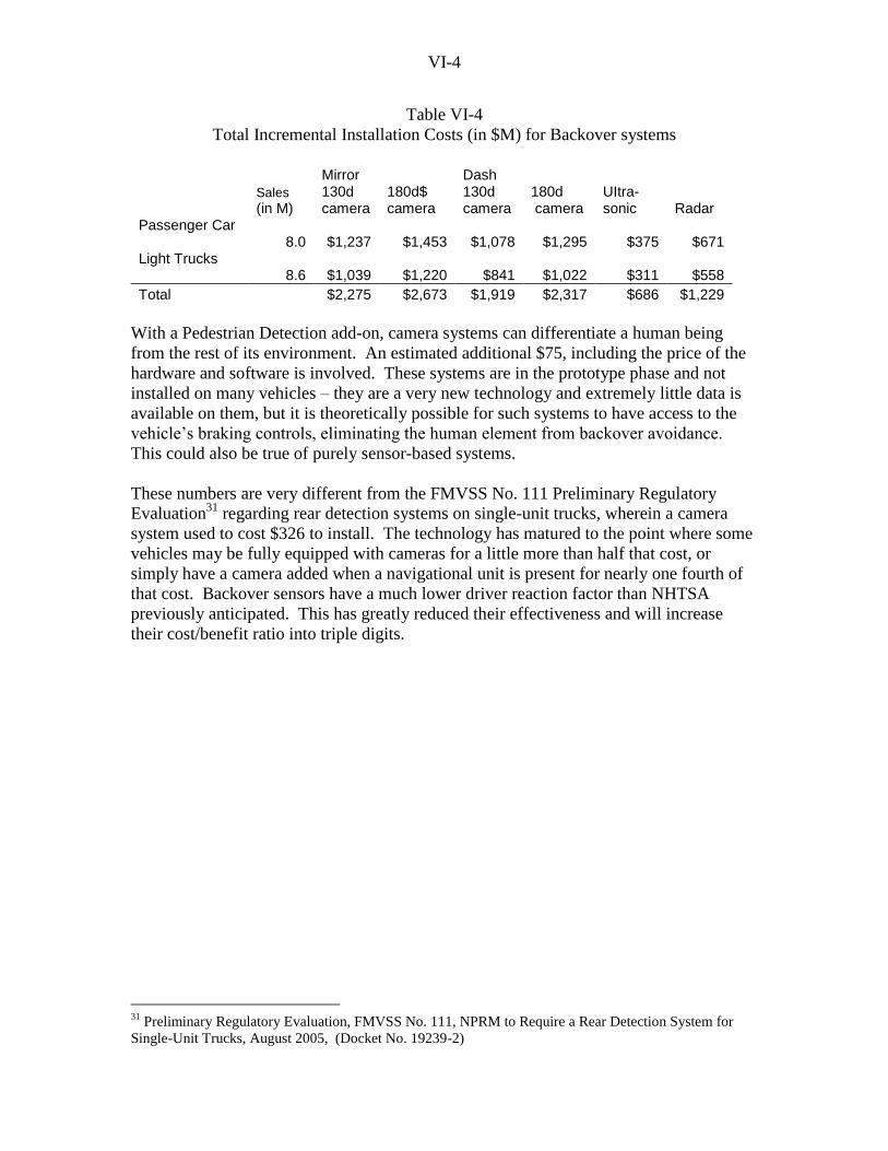
VI-4

Table VI-4

Total Incremental Installation Costs (in $M) for Backover systems

Mirror Dash

Sales (in M)

130d camera

180d$ camera

130d camera

180d camera

UItra-sonic Radar

Passenger Car 8.0 $1,237 $1,453 $1,078 $1,295 $375 $671 Light Trucks 8.6 $1,039 $1,220 $841 $1,022 $311 $558

Total $2,275 $2,673 $1,919 $2,317 $686 $1,229

With a Pedestrian Detection add-on, camera systems can differentiate a human being

from the rest of its environment. An estimated additional $75, including the price of the

hardware and software is involved. These systems are in the prototype phase and not

installed on many vehicles – they are a very new technology and extremely little data is

available on them, but it is theoretically possible for such systems to have access to the

vehicle‟s braking controls, eliminating the human element from backover avoidance.

This could also be true of purely sensor-based systems.

These numbers are very different from the FMVSS No. 111 Preliminary Regulatory

Evaluation31

regarding rear detection systems on single-unit trucks, wherein a camera

system used to cost $326 to install. The technology has matured to the point where some

vehicles may be fully equipped with cameras for a little more than half that cost, or

simply have a camera added when a navigational unit is present for nearly one fourth of

that cost. Backover sensors have a much lower driver reaction factor than NHTSA

previously anticipated. This has greatly reduced their effectiveness and will increase

their cost/benefit ratio into triple digits.

31

Preliminary Regulatory Evaluation, FMVSS No. 111, NPRM to Require a Rear Detection System for

Single-Unit Trucks, August 2005, (Docket No. 19239-2)

VII-1

VII. Cost Effectiveness & Benefit-Cost Analyses

The intent of the final rulemaking is to mitigate pedestrian backover crashes. This

section estimates the number of lives to be saved and injuries to be prevented per dollar

spent for the reduction in equivalent lives lost due to backover crashes. It should be

noted that the costs of the equipment needed to meet the requirements are incurred when

the vehicles are purchased, but the injury benefits and the property damage impacts of

rear visibility will accrue over the lifetime of the fleet. Therefore, discount factors are

applied to estimate the present value of injury benefits and property damage for a

meaningful comparison to costs.

Cost Effectiveness:

With respect to reduction in the number of fatalities and injuries, the agency estimates the

number of “equivalent fatalities” that would be prevented, or “equivalent lives saved,” a

concept that incorporates a reduction in both the number of fatalities and injuries. The

estimated equivalent lives saved and property damages prevented are discounted. The

costs are reduced by the amount of discounted property damage prevented to derive “net

costs.” These “net costs” are then compared to the estimated equivalent lives saved.

There is general agreement within the economic community that the appropriate basis for

determining discount rates is the marginal opportunity costs of lost or displaced funds.

When these funds involve capital investment, the marginal, real rate of return on capital

must be considered. However, when these funds represent lost consumption, the

appropriate measure is the rate at which society is willing to trade-off future for current

consumption. This is referred to as the "social rate of time preference," and it is generally

assumed that the consumption rate of interest, i.e., the real, after-tax rate of return on

widely available savings instruments or investment opportunities, is the appropriate

measure of its value.

Estimates of the social rate of time preference have been made by a number of authors.

Robert Lind TP

32PT estimated that the social rate of time preference is between zero and six

percent, reflecting the rates of return on Treasury bills and stock market portfolios. Kolb

and SheragaTP

33PT put the rate at between one and five percent, based on returns to stocks and

three-month Treasury bills. Moore and Viscusi TP

34PT calculated a two percent real time rate

of time preference for health, which they characterize as being consistent with financial

market rates for the period covered by their study. Moore and Viscusi's estimate was

TP

32PTLind, R.C., "A Primer on the Major Issues Relating to the Discount Rate for Evaluating National Energy

Options," in UDiscounting for Time and Risks in Energy Policy U, 1982, (Washington, D.C., Resources for the

Future, Inc.)

TP

33PTJ. Kolb and J.D. Sheraga, "A Suggested Approach for Discounting the Benefits and Costs of

Environmental Regulations,: unpublished working papers.

TP

34PTMoore, M.J. and Viscusi, W.K., "Discounting Environmental Health Risks: New Evidence and Policy

Implications," Journal of Environmental Economics and Management, V. 18, No. 2, March 1990, part 2 of

2.

VII-2

derived by estimating the implicit discount rate for deferred health benefits exhibited by

workers in their choice of job risk.

OMB Circular A-4 recommends agencies use both three percent and seven percent as the

“social rate of time preference”.

In the context of this particular regulatory evaluation of the efforts to improve rear

visibility in light vehicles, safety benefits occur when there is a potential crash severe

enough to result in occupant death or injury that would predictably be prevented by the

required technology. The benefits could occur at any time over the vehicle‟s lifetime.

This analysis assumes that crashes over the vehicle fleet‟s lifetime will occur in

proportion to the number of miles a given year‟s new vehicle fleet will be driven from

year to year as it ages. Tables VI-1a and VI-1b contain the vehicle miles of traveled

(VMT) by vehicle age and the survival probability schedules used in calculating age and

survival factors. The values in the column indicating the percentage of fleet travel that

would occur each year, i.e., weighted yearly travel, are used to distribute savings by year

of vehicle operation. The vehicle miles traveled (VMT) by vehicle age distribution is

used to determine the percentage of lifetime mileage that occurs each year that in turn is

used to calculate the discount factors by year for the three and seven percent discount

rates. The two right-hand columns show the weighted values for these discount factors.

These values are derived by multiplying the yearly discount factors by the share of

lifetime travel that occurs in the respective years and summing these factors over the 25

or 36 years. The values in the two columns are then summed to produce the following

multipliers for the respective discount rates:

For passenger cars, 0.8304 for a three percent discount rate and 0.6700 for a seven

percent discount rate, as shown in Table VII-1a.

For light trucks, 0.8022 for a three percent discount rate and 0.6303 for a seven percent

discount rate, as shown in Table VII-1b.

VII-3

Table VII-1a

Mid-Year Discount Factors, Passenger Cars

Age VMT (a) Survival

(b) (a) * (b)

% of VMT 3% 7%

Weighted 3%

Weighted 7%

1 14,231 0.99 14089 0.0926 0.9853 0.9667 0.0912 0.089518

2 13,961 0.9831 13725 0.0902 0.9566 0.9035 0.0863 0.0815

3 13,669 0.9731 13301 0.0874 0.9288 0.8444 0.0812 0.0738

4 13,357 0.9593 12813 0.0842 0.9017 0.7891 0.0759 0.0665

5 13,028 0.9413 12263 0.0806 0.8755 0.7375 0.0706 0.0594

6 12,683 0.9188 11653 0.0766 0.85 0.6893 0.0651 0.0528

7 12,325 0.8918 10991 0.0722 0.8252 0.6442 0.0596 0.0465

8 11,956 0.8604 10287 0.0676 0.8012 0.602 0.0542 0.0407

9 11,578 0.8252 9554 0.0628 0.7778 0.5626 0.0488 0.0353

10 11,193 0.7866 8804 0.0579 0.7552 0.5258 0.0437 0.0304

11 10,804 0.717 7746 0.0509 0.7332 0.4914 0.0373 0.0250

12 10,413 0.6125 6378 0.0419 0.7118 0.4593 0.0298 0.0193

13 10,022 0.5094 5105 0.0336 0.6911 0.4292 0.0232 0.0144

14 9,633 0.4142 3990 0.0262 0.671 0.4012 0.0176 0.0105

15 9,249 0.3308 3060 0.0201 0.6514 0.3749 0.0131 0.0075

16 8,871 0.2604 2310 0.0152 0.6324 0.3504 0.0096 0.0053

17 8,502 0.2028 1724 0.0113 0.614 0.3275 0.0070 0.0037

18 8,144 0.1565 1275 0.0084 0.5961 0.306 0.0050 0.0026

19 7,799 0.12 936 0.0062 0.5788 0.286 0.0036 0.0018

20 7,469 0.0916 684 0.0045 0.5619 0.2673 0.0025 0.0012

21 7,157 0.0696 498 0.0033 0.5456 0.2498 0.0018 0.0008

22 6,866 0.0527 362 0.0024 0.5297 0.2335 0.0013 0.0006

23 6,596 0.0399 263 0.0017 0.5142 0.2182 0.0009 0.0004

24 6,350 0.0301 191 0.0013 0.4993 0.2039 0.0006 0.0003

25 6,131 0.0227 139 0.0009 0.4847 0.1906 0.0004 0.0002

Total 152143 0.8304 0.6700

PT

VII-4

Table VII-1b

Mid-Year Discount Factors, Light Trucks T

Age VMT (a) Survival (b) (a) * (b) % of VMT 3% 7% Weighted 3% Weighted 7%

1 16,085 0.9741 15668 0.0871 0.9853 0.9667 0.0858 0.0842

2 15,782 0.9603 15155 0.0842 0.9566 0.9035 0.0806 0.0761

3 15,442 0.942 14546 0.0808 0.9288 0.8444 0.0751 0.0683

4 15,069 0.919 13848 0.0770 0.9017 0.7891 0.0694 0.0607

5 14,667 0.8913 13073 0.0726 0.8755 0.7375 0.0636 0.0536

6 14,239 0.859 12231 0.0680 0.85 0.6893 0.0578 0.0468

7 13,790 0.8226 11344 0.0630 0.8252 0.6442 0.0520 0.0406

8 13,323 0.7827 10428 0.0579 0.8012 0.602 0.0464 0.0349

9 12,844 0.7401 9506 0.0528 0.7778 0.5626 0.0411 0.0297

10 12,356 0.6956 8595 0.0478 0.7552 0.5258 0.0361 0.0251

11 11,863 0.6501 7712 0.0429 0.7332 0.4914 0.0314 0.0211

12 11,369 0.6042 6869 0.0382 0.7118 0.4593 0.0272 0.0175

13 10,879 0.5517 6002 0.0334 0.6911 0.4292 0.0230 0.0143

14 10,396 0.5009 5207 0.0289 0.671 0.4012 0.0194 0.0116

15 9,924 0.4522 4488 0.0249 0.6514 0.3749 0.0162 0.0093

16 9,468 0.4062 3846 0.0214 0.6324 0.3504 0.0135 0.0075

17 9,032 0.3633 3281 0.0182 0.614 0.3275 0.0112 0.0060

18 8,619 0.3236 2789 0.0155 0.5961 0.306 0.0092 0.0047

19 8,234 0.2873 2366 0.0131 0.5788 0.286 0.0076 0.0038

20 7,881 0.2542 2003 0.0111 0.5619 0.2673 0.0063 0.0030

21 7,565 0.2244 1698 0.0094 0.5456 0.2498 0.0051 0.0024

22 7,288 0.1975 1439 0.0080 0.5297 0.2335 0.0042 0.0019

23 7,055 0.1735 1224 0.0068 0.5142 0.2182 0.0035 0.0015

24 6,871 0.1522 1046 0.0058 0.4993 0.2039 0.0029 0.0012

25 6,739 0.1332 898 0.0050 0.4847 0.1906 0.0024 0.0010

26 6,663 0.1165 776 0.0043 0.4706 0.1781 0.0020 0.0008

27 6,648 0.1017 676 0.0038 0.4569 0.1665 0.0017 0.0006

28 6,648 0.0887 590 0.0033 0.4436 0.1556 0.0015 0.0005

29 6,648 0.0773 514 0.0029 0.4307 0.1454 0.0012 0.0004

30 6,648 0.0673 447 0.0025 0.4181 0.1359 0.0010 0.0003

31 6,648 0.0586 390 0.0022 0.4059 0.127 0.0009 0.0003

32 6,648 0.0509 338 0.0019 0.3941 0.1187 0.0007 0.0002

33 6,648 0.0443 295 0.0016 0.3826 0.1109 0.0006 0.0002

34 6,648 0.0385 256 0.0014 0.3715 0.1037 0.0005 0.0001

VII-5

35 6,648 0.0334 222 0.0012 0.3607 0.0969 0.0004 0.0001

36 6,648 0.029 193 0.0011 0.3502 0.0905 0.0004 0.0001

Total 179959 0.8022 0.6303

These multipliers are applied to the estimated number of equivalent fatalities prevented to

give the present values of estimated safety benefits for the respective discount rates.

A. Fatality and Injury Prevented Benefits:

As a primary measure of the impact of the rear visibility standard, this analysis will

measure the cost per equivalent life saved and also benefits in preventing property

damage involved in the crashes. In order to calculate a cost per equivalent fatality,

nonfatal injuries must be expressed in terms of fatalities. This is done by comparing the

value of preventing nonfatal injuries to the value of preventing a fatality. Comprehensive

values, which include both economic impacts and lost quality (or value) of life

considerations will be used to determine the relative values of fatalities and nonfatal

injuries. In the past, these values were taken from a study published by NHTSA when

the estimated economic value of preventing a human fatality was $3.0 million. TP

35PT In 2008,

the Department of Transportation has determined that the best current estimate of the

economic value of preventing a human fatality is $5.8 million in $2007. However,

relative value coefficients for preventing injuries of different severity have not been

developed. NHTSA is conducting research to revise the previously developed estimates.

The revised estimates will be published when they become available. In the interim, we

have adjusted the current estimates to reflect the revised $5.8 million statistical life for

both crash avoidance and crashworthiness Federal motor vehicle safety standards (see

Appendix A). Tables VII-2a and VII-2b show an example of how the comprehensive

values are used for each injury severity level, as well as the relative incident-based

weights for nonfatal injuries, AIS 1-5.

Table VII-2a

Process of Converting Nonfatal Injuries to Equivalent Fatalities

(Resulted from Rear Visibility Standard applied to Passenger Cars)

Injury Severity No. of Fatalities and

Injuries

Conversion Factor Equivalent Fatalities

(Undiscounted)

Fatalities 59 1.0000 59

AIS 5 29 0.6656 19

AIS 4 60 0.1998 12

AIS 3 420 0.0804 34

AIS 2 1162 0.0436 51

AIS 1 6,497 0.0028 18

Total 193

TP

35PT See Table A-1, The Economic Impact of Motor Vehicle Crashes 2000, DOT HS 809 446, NHTSA/DOT,

L. Blincoe, A. Seay, E. Zaloshnja, T. Miller, E.Romano, S. Luchter, R. Spicer, May, 2002.

VII-6

Table VII-2b

Process of Converting Nonfatal Injuries to Equivalent Fatalities

(Resulted from Rear Visibility Standard applied to Light Truck Vehicles)

Injury Severity No. of Fatalities and

Injuries

Conversion Factor Equivalent Fatalities

(Undiscounted)

Fatalities 169 1.0000 169

AIS 5 28 0.6656 19

AIS 4 57 0.1998 11

AIS 3 395 0.0804 32

AIS 2 1051 0.0436 46

AIS 1 5,589 0.0028 15

Total 292

The results in Tables VII-2a and -2b show that the installation of camera systems in

passenger cars would apply to a target population of 193 equivalent fatalities, whereas in

light truck vehicles it would apply to 292 equivalent fatalities.

PT

In Table VII-3, the safety benefits from Tables VII-2 have been discounted at three and

seven percent rates to express their present values over the lifetime of one model year‟s

production. The discount factors and the discounted target population fatal equivalents

are summarized in Table VII-3.

Table VII-3

Present Discounted Value of Fatalities within Target Population TP

36PT

(For equipping light vehicles with camera systems)

Fatal Equivalent Discount Rate Discounted Fatal Equivalent

193 (Pass. Cars) 0.8304 at 3% 160 0.6700 at 7% 129

292 (Light Trucks) 0.8022 at 3% 234 0.6303 at 7% 184

The discounted fatal equivalents in Tables VII-3 show that passenger car target

population is 129 equivalent lives discounted at seven percent and 160 equivalent lives

discounted at three percent.

B. Property Damage Prevented Benefits

Table VII-4, identical to Table VI-4 from the Cost section, presents the discounted values

of the estimated property damage prevented that the requirement would have on a per-

vehicle basis at the respective discount rates. As in the case for discounting the

equivalent fatality benefits, the numbers were derived by multiplying the estimated

amount of property damage prevented by the discount factors that were shown in Table

VII-3.

TP

36PT The discounted fatality numbers were rounded to the nearest integer.

VII-7

Table VII-4

Net Impacts per Vehicle from Property Damage and

Repair and Maintenance Costs ($2006) 55% fDR

17.5%

Backing 130 Camera

180 Camera

3% discount -$31.43 -$28.56

7% discount -$25.96 -$23.59

43% fDR

17.5%

Backing Ultrasonic Radar

3% discount $3.35 $5.50

7% discount $2.76 $4.54

C. Net Cost Per Equivalent Life Saved

The costs per equivalent life saved for light vehicles are computed using the annual net

cost figures (the sum of the installation costs from Chapter VI plus the discounted

property damage impacts above) and the discounted equivalent lives saved. All of the

calculations take into account the current installation rate, and thus benefits and costs are

both reduced to those generated by the rulemaking itself. These installation rates were

already produced for Table VI-2b, and the percentage of vehicles that need equipment are

multiplied by the appropriate sales numbers, and then these products (in “number of

cars”) is multiplied by either the installation cost (per car) or the per-car impact from

Property Damage to generate the corresponding values. Calculations have been made for

the various technologies at the 3% and 7% discount factor. The following tables detail

the equivalent lives saved, installation cost (the cost to implement the rulemaking by

installing the devices), lifetime cost (installation costs plus the impacts from Property

Damage and Repair and Maintenance, found in table VII-4 above), and cost per

equivalent life saved for all considered.

VII-8

Table VII-5a

Equivalent Lives Saved, Net Cost, and Cost per Equivalent Life Saved for Backover

Systems at the 3% and 7% Discount Rate

Passenger Cars and Light Trucks

Equivalent Lives Saved 3% discount rate

Installation Costs (in $M)

Lifetime Costs (incl. PDO crashes) (in $M) 3% discount rate

Net Cost/EQ Life Saved (in $M)

130 Mirror 127.4 $2,275.3 $1,861.3 14.6

130 Dash 127.4 $1,919.2 $1,505.1 11.8

180 Mirror 150.8 $2,673.1 $2,296.9 15.2

180 Dash 150.8 $2,316.9 $1,940.7 12.9

Ultrasonic 7.6 $685.8 $730.4 95.5

Radar 8.4 $1,228.8 $1,302.1 154.5

Equivalent Lives Saved 7% discount rate

Installation Costs (in $M)

Lifetime Costs (incl. PDO crashes) (in $M) 7% discount rate

Net Cost/EQ Life Saved (in $M)

130 Mirror 101.3 $2,275.3 $1,933.3 19.1

130 Dash 101.3 $1,919.2 $1,577.2 15.6

180 Mirror 120.0 $2,673.1 $2,362.4 19.7

180 Dash 120.0 $2,316.9 $2,006.2 16.7

Ultrasonic 6.1 $685.8 $722.6 118.8

Radar 6.7 $1,228.8 $1,289.4 192.3

From all of these values, we find that the lowest estimated cost per equivalent life saved

for cameras requires a 130 degree dash-display camera system, at the 3 percent discount

level, and would cost an approximate $11.8 million per equivalent life saved. The

highest camera estimate requires a 180 degree mirror-display camera system, at the 7

percent discount level, and would cost an approximate $19.7 million per equivalent life

saved. The lowest cost per equivalent life saved for sensor systems was $86.7 per life

saved, equipping ultrasonic systems at the 3 percent discount level. However, the highest

cost per equivalent lives saved for sensors was the radar system at the 7% discount level,

providing a cost of $211.9 million per life saved. For perspective, NHTSA estimates a

cost of $6.1 million per statistical life when valuing a reduction in premature fatalities, so

none of these systems are cost effective.

While a rulemaking that only requires light trucks to be equipped is within scope,

NHTSA is not proposing at this time that the fleet be equipped based on vehicle type.

Below are the costs and benefits for such an alternative.

VII-9

Table VII-5b

Equivalent Lives Saved, Net Cost, and Cost per Equivalent Life Saved for Backover

Systems at the 3% and 7% Discount Rate, by Vehicle Type

Equivalent Lives Saved Lifetime Costs, including PDO crashes (in $M)

PC Only 3% discount rate

Installation Costs (in $M)

3% discount rate

Net Cost/EQ Life Saved (in $M)

130 Mirror 59.4 $1,236.6 $1,011.6 $17.0

130 Dash 59.4 $1,078.4 $853.4 $14.4

180 Mirror 70.3 $1,452.8 $1,248.3 $17.7

180 Dash 70.3 $1,294.6 $1,090.2 $15.5

Ultrasonic 3.6 374.5 398.9 $111.2

Radar 4.0 671.1 711.1 $180.0

LT Only

130 Mirror 68.0 $1,038.7 $849.7 $12.5

130 Dash 68.0 $840.7 $651.7 $9.6

180 Mirror 80.5 $1,220.3 $1,048.6 $13.0

180 Dash 80.5 $1,022.3 $850.6 $10.6

Ultrasonic 4.1 $311.3 $331.5 $81.6

Radar 4.5 $557.8 $591.0 $132.1

Equivalent Lives Saved Lifetime Costs, including PDO crashes (in $M)

PC Only 7% discount rate

Installation Costs (in $M)

7% discount rate

Net Cost/EQ Life Saved (in $M)

130 Mirror 47.9 $1,236.6 $1,050.8 $21.9

130 Dash 47.9 $1,078.4 $892.6 $18.6

180 Mirror 56.7 $1,452.8 $1,283.9 $22.6

180 Dash 56.7 $1,294.6 $1,125.8 $19.8

Ultrasonic 2.9 374.5 394.6 $136.4

Radar 3.2 671.1 704.1 $220.9

LT Only

130 Mirror 53.4 $1,038.7 $882.6 $16.5

130 Dash 53.4 $840.7 $684.6 $12.8

180 Mirror 63.3 $1,220.3 $1,078.4 $17.0

180 Dash 63.3 $1,022.3 $880.5 $13.9

Ultrasonic 3.2 $311.3 $328.0 $102.8

Radar 3.5 $557.8 $585.2 $166.4

D. Benefit-Cost Analysis

Effective January 1, 2004, OMB Circular A-4 requires that analyses performed in support

of final rules must include both cost effectiveness and benefit-cost analysis. Benefit-cost

analysis differs from cost effectiveness analysis in that it requires that benefits be

assigned a monetary value, and that this value be compared to the monetary values of

costs to derive an estimate of net benefit. In valuing reductions in premature fatalities,

we used a NHTSA value of $6.1 million based on a value of $5.8 million per statistical

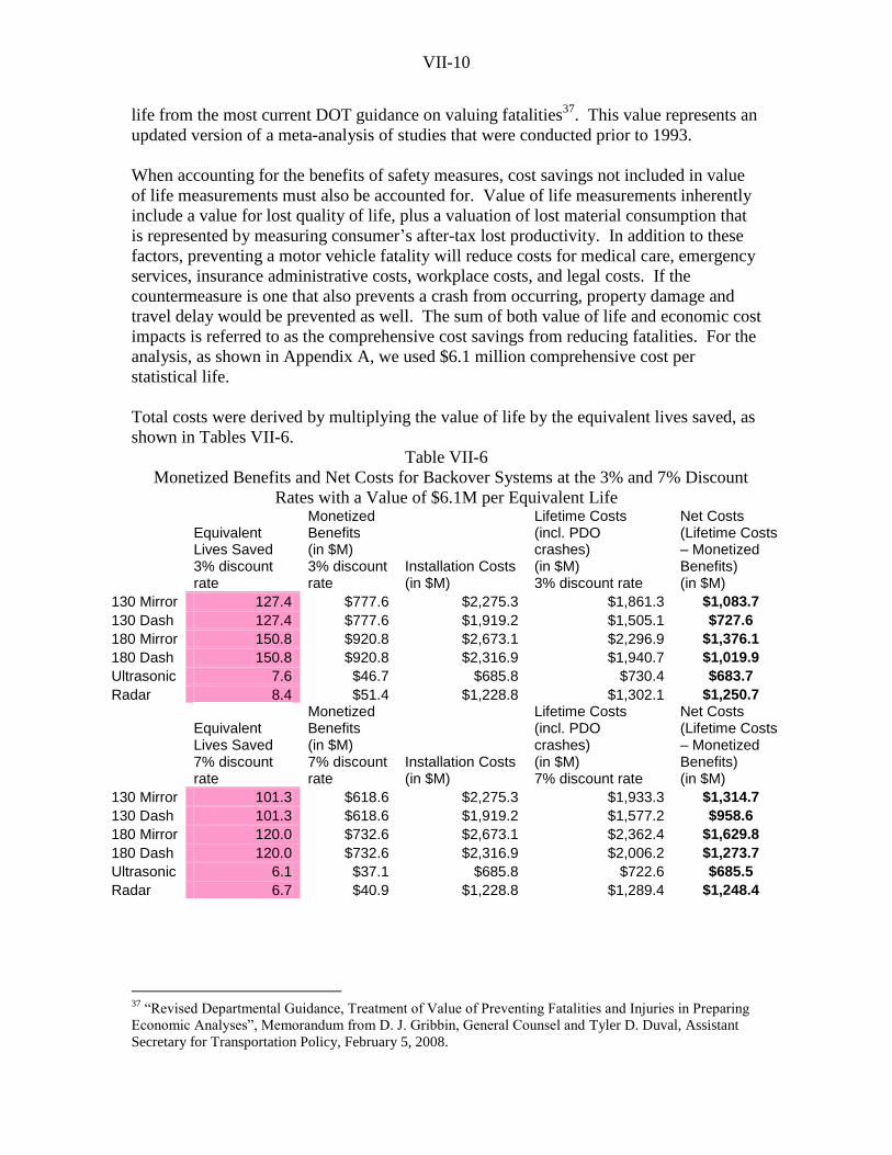
VII-10

life from the most current DOT guidance on valuing fatalities TP

37PT. This value represents an

updated version of a meta-analysis of studies that were conducted prior to 1993.

When accounting for the benefits of safety measures, cost savings not included in value

of life measurements must also be accounted for. Value of life measurements inherently

include a value for lost quality of life, plus a valuation of lost material consumption that

is represented by measuring consumer‟s after-tax lost productivity. In addition to these

factors, preventing a motor vehicle fatality will reduce costs for medical care, emergency

services, insurance administrative costs, workplace costs, and legal costs. If the

countermeasure is one that also prevents a crash from occurring, property damage and

travel delay would be prevented as well. The sum of both value of life and economic cost

impacts is referred to as the comprehensive cost savings from reducing fatalities. For the

analysis, as shown in Appendix A, we used $6.1 million comprehensive cost per

statistical life.

Total costs were derived by multiplying the value of life by the equivalent lives saved, as

shown in Tables VII-6.

Table VII-6

Monetized Benefits and Net Costs for Backover Systems at the 3% and 7% Discount

Rates with a Value of $6.1M per Equivalent Life

Equivalent Lives Saved 3% discount rate

Monetized Benefits (in $M) 3% discount rate

Installation Costs (in $M)

Lifetime Costs (incl. PDO crashes) (in $M) 3% discount rate

Net Costs (Lifetime Costs – Monetized Benefits) (in $M)

130 Mirror 127.4 $777.6 $2,275.3 $1,861.3 $1,083.7

130 Dash 127.4 $777.6 $1,919.2 $1,505.1 $727.6

180 Mirror 150.8 $920.8 $2,673.1 $2,296.9 $1,376.1

180 Dash 150.8 $920.8 $2,316.9 $1,940.7 $1,019.9

Ultrasonic 7.6 $46.7 $685.8 $730.4 $683.7

Radar 8.4 $51.4 $1,228.8 $1,302.1 $1,250.7

Equivalent Lives Saved 7% discount rate

Monetized Benefits (in $M) 7% discount rate

Installation Costs (in $M)

Lifetime Costs (incl. PDO crashes) (in $M) 7% discount rate

Net Costs (Lifetime Costs – Monetized Benefits) (in $M)

130 Mirror 101.3 $618.6 $2,275.3 $1,933.3 $1,314.7

130 Dash 101.3 $618.6 $1,919.2 $1,577.2 $958.6

180 Mirror 120.0 $732.6 $2,673.1 $2,362.4 $1,629.8

180 Dash 120.0 $732.6 $2,316.9 $2,006.2 $1,273.7

Ultrasonic 6.1 $37.1 $685.8 $722.6 $685.5

Radar 6.7 $40.9 $1,228.8 $1,289.4 $1,248.4

TP

37PT “Revised Departmental Guidance, Treatment of Value of Preventing Fatalities and Injuries in Preparing

Economic Analyses”, Memorandum from D. J. Gribbin, General Counsel and Tyler D. Duval, Assistant

Secretary for Transportation Policy, February 5, 2008.

VII-11

Our analysis of rear visibility results in costs that outweigh the benefits given the current

technology and our understanding of the target population and installation rates. A

reduction in lives lost to and injuries caused by backover accidents, in addition to benefits

from property damage only crashes, are expected, but the combination of the monetized

benefits and the cost of implementation and maintenance are a net cost between $236

million and $1.6 billion.

E. Potential Alternatives

In order to explore fully other possible rulemaking options, a variety of combinations of

technology were examined, specifically, ones in which light trucks were equipped with a

camera system, and passenger cars were given no extra equipment, a similar camera,

radar, or ultrasonic systems. The results of examining such combinations are available

below. Note the camera/radar and camera/ultrasonic options have decreased costs

compared to mandating cameras for both vehicle types, but have a higher cost per life

saved. It would not fulfill the requirements of the statute to require cameras for light

trucks and nothing for passenger cars; those numbers are provided only as a point of

comparison. Also, the camera/radar option has a higher net cost associated with it than

simply mandating cameras for both, and will most likely not be viable on those grounds.

Comments on these alternatives and suggestions of others are welcome.

Rear Visibility Options

Discounted at 3%

($Millions of 2007)

Installation

Costs*

Monetized

Benefits

Property

Damage

Costs

Net

Costs

Net Cost per

Equivalent

Life Saved

LT Camera

PC Camera

$1,919 to

$2,275

$778 $ -414 $727 to

$1,084

$11.8 to

$14.6

LT Camera

PC Radar

$1,512 to

$1,710

$439 $ -149 $924 to

$1,122

$18.9 to

$21.7

LT Camera

PC Ultrasonic

$1,215 to

$1,413

$437 $ -165 $613 to

$811

$14.7 to

$17.4

LT Camera

PC Nothing

$841 to

$1,039

$415 $ -189 $237 to

$435

$9.6 to

$12.5

*The range of camera costs assumes 130 degree camera with the display in the dash (lower cost)

to the display in the mirror (higher cost)

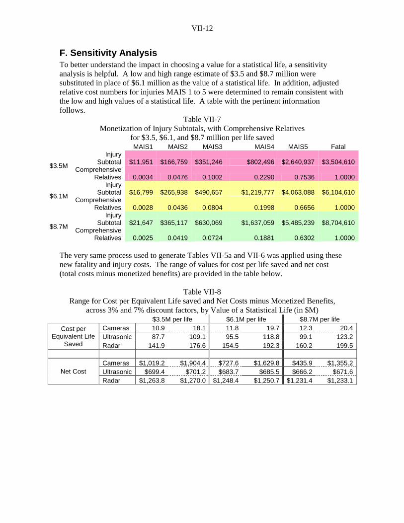
VII-12

F. Sensitivity Analysis

To better understand the impact in choosing a value for a statistical life, a sensitivity

analysis is helpful. A low and high range estimate of $3.5 and $8.7 million were

substituted in place of $6.1 million as the value of a statistical life. In addition, adjusted

relative cost numbers for injuries MAIS 1 to 5 were determined to remain consistent with

the low and high values of a statistical life. A table with the pertinent information

follows.

Table VII-7

Monetization of Injury Subtotals, with Comprehensive Relatives

for $3.5, $6.1, and $8.7 million per life saved MAIS1 MAIS2 MAIS3 MAIS4 MAIS5 Fatal

$3.5M

Injury Subtotal $11,951 $166,759 $351,246 $802,496 $2,640,937 $3,504,610

Comprehensive Relatives 0.0034 0.0476 0.1002 0.2290 0.7536 1.0000

$6.1M

Injury Subtotal $16,799 $265,938 $490,657 $1,219,777 $4,063,088 $6,104,610

Comprehensive Relatives 0.0028 0.0436 0.0804 0.1998 0.6656 1.0000

$8.7M

Injury Subtotal $21,647 $365,117 $630,069 $1,637,059 $5,485,239 $8,704,610

Comprehensive Relatives 0.0025 0.0419 0.0724 0.1881 0.6302 1.0000

The very same process used to generate Tables VII-5a and VII-6 was applied using these

new fatality and injury costs. The range of values for cost per life saved and net cost

(total costs minus monetized benefits) are provided in the table below.

Table VII-8

Range for Cost per Equivalent Life saved and Net Costs minus Monetized Benefits,

across 3% and 7% discount factors, by Value of a Statistical Life (in $M) $3.5M per life $6.1M per life $8.7M per life

Cost per Equivalent Life

Saved

Cameras 10.9 18.1 11.8 19.7 12.3 20.4

Ultrasonic 87.7 109.1 95.5 118.8 99.1 123.2

Radar 141.9 176.6 154.5 192.3 160.2 199.5

Net Cost

Cameras $1,019.2 $1,904.4 $727.6 $1,629.8 $435.9 $1,355.2

Ultrasonic $699.4 $701.2 $683.7 $685.5 $666.2 $671.6

Radar $1,263.8 $1,270.0 $1,248.4 $1,250.7 $1,231.4 $1,233.1

VIII-1

VIII. Regulatory Flexibility Act and Unfunded Mandates Reform Act Analysis

A. Regulatory Flexibility Act

The Regulatory Flexibility Act of 1980 (5 U.S.C §601 et seq.) requires agencies to

evaluate the potential effects of their proposed and final rules on small business, small

organizations and small Government jurisdictions.

5 U.S.C §603 requires agencies to prepare and make available for public comments initial

and final regulatory flexibility analysis (RFA) describing the impact of proposed and

final rules on small entities. Section 603(b) of the Act specifies the content of a RFA.

Each RFA must contain:

1. A description of the reasons why action by the agency is being considered;

2. A succinct statement of the objectives of, and legal basis for a final rule;

3. A description of and, where feasible, an estimate of the number of small entities

to which the final rule will apply;

4. A description of the projected reporting, recording keeping and other compliance

requirements of a final rule including an estimate of the classes of small entities

which will be subject to the requirement and the type of professional skills

necessary for preparation of the report or record;

5. An identification, to the extent practicable, of all relevant Federal rules which

may duplicate, overlap or conflict with the final rule;

6. Each regulatory flexibility analysis shall also contain a description of any

significant alternatives which accomplish the stated objectives of applicable

statutes and which minimize any significant economic impact on small entities.

1. Description of the reason why action by the agency is being considered

NHTSA is proposing this action to carry out the requirements of the Cameron

Gulbransen Kids Transportation Safety Act of 2007.

2. Objectives of, and legal basis for, the final rule

The Act requires the agency to conduct rulemaking to expand the required field of view

to prevent backover incidents.

3. Description and estimate of the number of small entities to which the final rule will

apply

The final rule will affect motor vehicle manufacturers. There are no light truck

manufacturers that are small businesses. However, there are six domestically owned

small passenger car manufacturers.

Business entities are defined as small business using the North American Industry

Classification System (NAICS) code, for the purpose of receiving Small Business

Administration assistance. One of the criteria for determining size, as stated in 13 CFR

121.201, is the number of employees in the firm. For establishments primarily engaged

VIII-2

in manufacturing or assembling automobiles, light and heavy duty trucks, buses, motor

homes, or motor vehicle body manufacturing, the firm must have less than 1,000

employees to be classified as a small business.

We believe that the rulemaking would not have a significant economic impact on the

small vehicle manufacturers because the systems are not technically hard to develop or

install and the cost of the systems ($160 to $200) is a small proportion (less than half of

one percent) of the overall vehicle cost for most of these specialty cars. The exception is

Standard Taxi ($200/$25,000 = 0.8 percent of the sales price). Since every manufacturer

needs to meet the standard, the proposal would have no effect on competition. However,

it does raise the overall cost, and could affect sales in a small way.

Currently, there are six small passenger car motor vehicle manufacturers in the United

States. Table VIII-1 provides information about the 6 small domestic manufacturers in

MY 2007. All are small manufacturers, having much less than 1,000 employees.

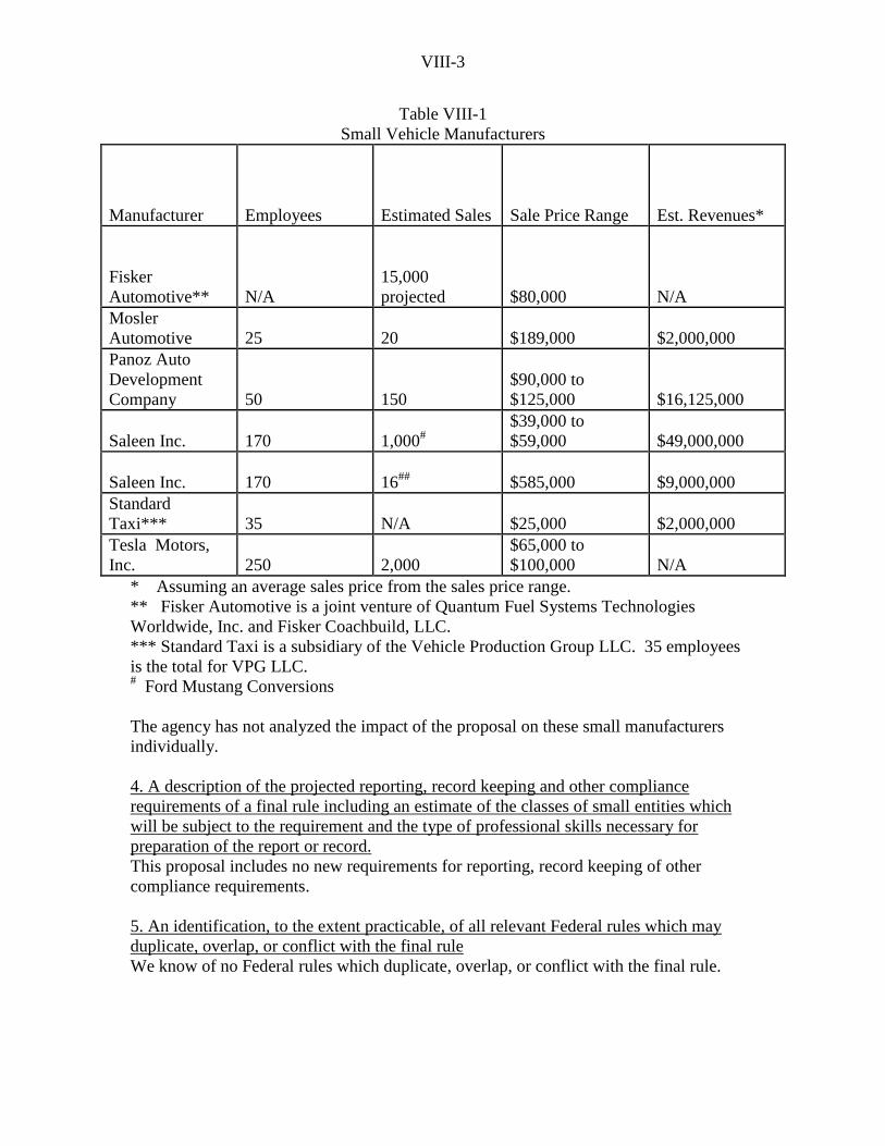
VIII-3

Table VIII-1

Small Vehicle Manufacturers

Manufacturer

Employees

Estimated Sales

Sale Price Range

Est. Revenues*

Fisker

Automotive**

N/A

15,000

projected

$80,000

N/A

Mosler

Automotive

25

20

$189,000

$2,000,000

Panoz Auto

Development

Company

50

150

$90,000 to

$125,000

$16,125,000

Saleen Inc.

170

1,000#

$39,000 to

$59,000

$49,000,000

Saleen Inc.

170

16##

$585,000

$9,000,000

Standard

Taxi***

35

N/A

$25,000

$2,000,000

Tesla Motors,

Inc.

250

2,000

$65,000 to

$100,000

N/A

* Assuming an average sales price from the sales price range.

** Fisker Automotive is a joint venture of Quantum Fuel Systems Technologies

Worldwide, Inc. and Fisker Coachbuild, LLC.

*** Standard Taxi is a subsidiary of the Vehicle Production Group LLC. 35 employees

is the total for VPG LLC. # Ford Mustang Conversions

The agency has not analyzed the impact of the proposal on these small manufacturers

individually.

4. A description of the projected reporting, record keeping and other compliance

requirements of a final rule including an estimate of the classes of small entities which

will be subject to the requirement and the type of professional skills necessary for

preparation of the report or record.

This proposal includes no new requirements for reporting, record keeping of other

compliance requirements.

5. An identification, to the extent practicable, of all relevant Federal rules which may

duplicate, overlap, or conflict with the final rule

We know of no Federal rules which duplicate, overlap, or conflict with the final rule.

VIII-4

6. A description of any significant alternatives to the final rule which accomplish the

stated objectives of applicable statutes and which minimize any significant economic

impact of the proposal on small entities.

The agency is considering a variety of alternatives and knows of no other alternatives that

can achieve the stated objectives and minimize the impacts on small entities.

B. Unfunded Mandates Reform Act

The Unfunded Mandates Reform Act of 1995 (Public Law 104-4) requires agencies to

prepare a written assessment of the costs, benefits, and other effects of proposed or final

rules that include a Federal mandate likely to result in the expenditures by States, local or

tribal governments, in the aggregate, or by the private sector, of more than $100 million

annually (adjusted annually for inflation with base year of 1995). Adjusting this amount

by the implicit gross domestic product price deflator for 2007 results in $130 million

(119.816/92.106 = 1.30). The assessment may be included in conjunction with other

assessments, as it is here.

IX-1

IX. Probabilistic Uncertainty Analysis

This chapter identifies and quantifies the major uncertainties in the cost-effectiveness and

net benefit analyses and examines the impacts of these uncertainties. Throughout the

course of these analyses, many assumptions were made, diverse data sources were used,

and different statistical processes were applied. The variability of these assumptions,

data sources, and statistical processes potentially would influence the estimated

regulatory outcomes. Thus, all these assumptions, data sources, and derived statistics can

be considered as uncertainty factors for the regulatory analysis. The purpose of this

uncertainty analysis is to identify the uncertainty factors with appreciable variability,

quantify these uncertainty factors by appropriate probability distributions, and induce the

probabilistic outcomes accompanied with degrees of probability or plausibility. This

facilitates a more informed decision-making process.

A Monte Carlo statistical simulation technique38

is used to accomplish the process. The

technique is to first randomly select values for those uncertainty factors from their pre-

established probability distributions. The selected values then are fed back to the cost-

effectiveness and net benefit analysis process to generate all possible outcomes. The

process is run repeatedly. Each complete run is a trial. Crystal Ball®39

, a spreadsheet-

based risk analysis and forecasting software package which includes the Monte Carlo

simulation technique tool, was chosen to automate the process. In addition to simulation

results, Crystal Ball® also provides the degree of certainty (or confidence, or credibility)

that is associated with the simulated results. The degree of certainty provides the

decision-makers an additional piece of important information to evaluate the outcomes.

The analysis starts by establishing mathematical models that imitate the actual processes

in deriving cost-effectiveness and net benefits, as shown in previous chapters. The

formulation of the models also allows analysts to conveniently identify and categorize

uncertainty factors. In the mathematical model, each variable (e.g., cost of technology)

represents an uncertainty factor that would potentially alter the model outcomes if its

value were changed. Variations of these uncertainty factors are described by appropriate

probability distribution functions. These probability distributions are established based

on available data. If data are not sufficient or not available, professional judgments are

used to estimate the distribution of these uncertainty factors.

After defining and quantifying the uncertainty factors, the next step is to simulate the

model to obtain probabilistic results rather than single-value estimates. The simulation

38

See a: Robert, C.P. & Casella, G., Monte Carlo Statistical Methods, Springer-Verlag New York, Inc.,

1999, and

b: Liu, J.S., Monte Carlo Strategies in Scientific Computing, Springer-Verlag New York, Inc., 2001

(Or any statistics books describing the Monte Carlo simulation theory are good references for

understanding the technique).

39

A registered trademark of Decisioneering, Inc. (now a unit of Oracle company)

IX-2

repeats the trials until certain pre-defined criteria40

are met and a probability distribution

of results is generated. Note that the uncertainty analysis did not examine the technology

“look-down mirrors” since the mean benefit estimated in the previous chapter is 0.

A. Simulation Models

Mathematical models were built to imitate the process used in deriving cost-effectiveness

and net benefits as developed in previous chapters. Both the cost-effectiveness and net

benefit models comprise three principal components: injury benefits, property damage

savings/costs, and vehicle technology costs. These three components are discussed

separately in the following sections.

A.1 Injury Benefit Component

In the cost-effectiveness model, injury benefits are represented by fatal equivalents (FEs)

reduced. In the net benefit model, injury benefits are represented by their monetary

value, which is the product of comprehensive cost per life saved and FEs. Since benefits

(fatalities and injuries reduced) were already expressed as FEs in the cost-effectiveness

model, the net benefit model is just one step removed from the cost-effectiveness model.

Therefore, the FE model is discussed first.

FEs is derived through the following steps:

1. Establishing baseline fatal and injury populations

2. Deriving initial injury benefits (i.e., fatalities and MAIS 1-5 injuries eliminated

by the proposal),

3. Adjusting the initial injury benefits to account for technology installation rate for

MY 2010 fleet passenger vehicles (2010-based adjustment factor)

4. Deriving FEs by multiplying the injury benefits by their corresponding injury-to-

fatality ratios, and

5. Discounting FEs to derive the discounted net benefits over the vehicle‟s life.

Therefore, FEs can be represented by the following mathematical formula for each of the

technologies examined in the PRIA:

40

The pre-defined criteria may change with each uncertainty analysis. In this case, we require a 99 percent

precision in mean for each simulated outcome such as total costs, cost-effectiveness, and net benefits as

described later.

IX-3

(1) ----- d*a*]r *e*T[FEs ii

6

1j

jij

2

1i

Where,

Tij = target population, i=1 for PCs and i=2 for LTVs; j=1 as MAIS j injuries with

j=6 as fatalities

e = effectiveness of the technology against the target population

rj = MAIS j injury-to-fatality ratio with j=6 as fatalities

ai = 2010-based adjustment factor

di = cumulative lifetime discount factor, either at 3 or 7 percent discount rate.

The effectiveness “e” defined here is essentially the product of three independent factors:

(1) the percentage of cases that were found to be “avoidable”, i.e., avoidability ( fA), the

percentage of cases in which the system performs and provides the needed information

(fS), and the percentage of cases where drivers will recognize the information from the

system and act appropriately to actually avoid a crash (fDR). Therefore, e can be further

expanded as:

e = fA * fS * fDR

Also, ai, the 2010-based adjustment factor is basically equal to 1 minus the technology

installation rate in MY 2010 passenger vehicle fleet.

The product of the target population (Tij) and the corresponding technology effectiveness

rate (e) represents the initial injury severity j benefits for the ith

vehicle type (= Tij*e =

Tij* fA * fS * fDR). Multiplying the injury severity j benefits by its corresponding injury-

to-fatality ratio [= Tij*e * ri]) derives its FEs. Summed over the injury severity (index j)

thus derives the total FEs for the ith

vehicle type type (=6

1j

jij r *e*T ). The initial FEs

then were adjusted to 2010 level to account for technology installation rate by

multiplying it by the 2010-based adjustment factor ai [=6

1j

jij r *e*T * ai)]. Finally, the

total FEs are discounted either at a 3 or 7 percent rate to reflect the net benefits of the rule

over a vehicle‟s life.

FEs is the basic benefit measurement for estimating cost-effectiveness. For net benefits,

FEs are translated into monetary value. If M denotes the cost per fatality, benefit in the

net benefit calculation is equal to M*FEs. Hence, the benefit component for net benefits

is:

ii

6

1j

jDRSAij

2

1i

ii

6

1j

jij

2

1i

d*a*]r*f*f*f*T[*M

d*a*]r*e*T[*MFEs*M

IX-4

A.2 Lifetime Property Damage Savings (S)

Property damage savings include the benefits of eliminating backing over crashes and the

costs for technology repair/maintenance from property damage only and rear-end crashes.

Property damage savings are realized over a vehicle‟s life and would be discounted at 3

and 7 percent. Therefore, S can be represented by the following mathematical formula:

2

1i

iii a * v*uS

Where,

ui = discounted (at 3 or 7 percent) unit lifetime property damage savings for

affected

vehicles, with i=1 as PCs and j=2 as LTVs

vi = number of new vehicles

ai = 2010-based adjustment factor.

A.3 Vehicle Technology Cost Component

Vehicle technology cost (VC) is the product of technology cost per affected vehicle and

the number of affected vehicles. The number of affected vehicles can be derived by

multiplying the total number of new vehicles and the proportion of vehicles that need to

install the technology (i.e., number of new vehicles * 2010-based adjustment factor).

The 2010-based adjustment factor used in the cost component is further segregated by

implementation options (full or partial system). The vehicle technology cost of the

proposal can be represented as: 2

1i

2

1j

ijiij a *v*cVC

Where, VC = vehicle technology cost

cij = technology cost per affected vehicle, i=1 for PCs and i=2 for LTVs;

j=1 for full system and j=2 for partial system

vi = number of new vehicles

aij = 2010-based adjustment factor.

Note that, the 2010-based adjustment factor ai used in the FE model is the sum of

corresponding full (ai1) and partial system adjustment factor (ai2), i.e., ai = ai1 + ai2. The

full and partial systems primarily are for camera systems. A full system includes a

camera and a display system. A partial system only includes a camera. The partial

system would be required for vehicles that already are equipped with an in-dash

navigation unit.

A.4 Cost-Effectiveness Model and Net Benefit Model

After the fatal equivalents, property damage savings/costs, and vehicle technology cost

were established, the cost-effectiveness model (CE) is calculated as the ratio of net costs

IX-5

(NC) to fatal equivalents (FEs) where NC is equal to vehicle technology cost (VC) minus

lifetime property damage savings (S). The cost-effectiveness model (CE) has the format:

FEs

SVC

FEs

NCCE

The net benefit is the difference between benefits expressed in monetary value and the

net cost. Thus, the net benefit model (NB) has the format:

VCSFEs*M

NCFEs*MNB

Where, M is the cost per fatality.

B. Uncertainty Factors

Each parameter in the above cost-effectiveness and net benefit model represents a major

category of uncertainty factors. Therefore, there are ten major categories of uncertainty

factors that would impact the cost-effectiveness: (1) target crash population, Tij, (2)

avoidability, fA, (3) system performance factor, fS, (4) driver factor, fDR, (5) 2010-based

adjustment factors aij, (6) injury-to-fatality ratios, ri, (7) cumulative lifetime discount

factors, di, (8) discounted unit lifetime property damage savings, ui, (9) technology cost

per affected vehicle, ci, and (10) number of new vehicles, vi. The net benefit model has

one additional uncertainty factor (11) cost per life, M, in addition to ten for the cost-

effectiveness model.

Target population, Tij, is important to benefit estimates because it defines the crash

population of risk without the proposal. Fatal and injury target populations were derived

from three data systems: FARS, GES, and NiTS. The major uncertainties in this factor

arise from reporting errors in NiTS and survey errors in GES. The reporting errors in

NiTS are not available due to the lack of an established off-roadway crash baseline to

which NiTS can be compared. Consequently, the overall variation of the target

population is unknown. However, given that NiTS has sufficient sample and that

sampling systems including GES generally allow a 5 percent sampling error, a normal

distribution with a standard error as 10 percent of the mean is considered sufficient to

describe variations of the target populations.

Note that probability functions for target fatal and MAIS injury populations cannot be

established independently because their relative ratios are expected to regress to the mean

relative ratios as reported in the crash databases. To address this interdependency issue,

the analysis first established the variation for the overall target population (i.e., all injury

and fatalities). After establishing the variation (i.e., a normal distribution with 10 percent

of the mean as one standard deviation), the overall target population was distributed into

fatalities and MAIS injuries. The distribution was based on their mean proportions.

These mean proportions are treated as constants.

IX-6

Avoidability fA, is significant since it would affect the effectiveness of the proposed

technology. The sources of its uncertainty include the bias inherent in the expert

judgments and the representativeness of cases where fA were derived from. Since a team

of reviewers first accessed the value of fA independently for each of the selected cases

and then they jointly resolved any discrepancies, the point estimate of fA for each case is

considered to be a fair assessment. Furthermore, the sample cases that were reviewed by

the team are adequate to represent backing over crashes. Therefore, the agency believes

that the range between the avoidable percentage and the combined percentage of

“avoidable”, “possibly avoidable”, and “possibly not avoidable” is sufficient to capture

the variation for fA. In order words, for each technology examined by the PRIA, the

value of fA would fall between these two percentages.

Due to the range constraint, beta probability distributions are chosen to describe the

variations for fA for its flexibility and capability of setting distribution boundary. In

addition to lower and higher bounds, a beta distribution has two more parameters, α and

β, that determine the shape of the beta distribution. The values of α and β were

established by setting the mean of the distribution as the combined percentage of

“avoidable” and “possibly avoidable” cases.

System performance factor, fS, addresses the limitation of the technologies and would

also affect the effectiveness of technologies. However, this factor is primarily used in

determining the reliability of sensor-based systems such as ultrasonic and radar systems.

It would not affect the camera systems. Sources of uncertainty for fS include

experimental errors and production variation. Based on expert assessment and the

agency‟s experience with manufacturers‟ production reliability of vehicle safety systems,

a 10 percent performance variation is considered to be sufficient to account for the

majority of the uncertainties associated with fS. Any value within this range is expected

to have an equal chance to be the true system performance. Thus, the analysis treats fS as

uniformly distributed for the ultrasonic and radar systems. It is treated as constant with

value of 1 since it does not impact the camera systems.

Driver factor, fDR, also affects the effectiveness of the technologies examined in the

PRIA. The sources of its uncertainty include, but are not limited to, experimental errors,

representativeness of drivers used for the experiment, driving environment, and driver

conditions. Variations for these uncertainty sources are unknown. Nevertheless, the

analysis treats the values of fDR as normally distributed to account for the impact of this

factor. One standard deviation is set to be 10 percent of the mean.

2010-based adjustment factors, aij, are used to adjust the initial benefits and costs to 2010

level. The source of its uncertainty primarily is from projection errors. Since, aij would

impact both benefits and costs of the proposal in similar magnitude. Variations for these

factors thus would not be expected to increase the uncertainty level for cost-effectiveness

and net benefit measurements. Therefore, this factor is treated as a constant.

Injury-to-fatality ratios, rj, reflect the relative economic impact of injuries compared to

fatalities based on their estimated comprehensive unit costs. They were derived based on

IX-7

the 2007 update of the most current 2002 crash cost assessment41

. The crash cost

assessment itself is a complex analysis with an associated degree of uncertainty. At this

time, these uncertainties are also unknowns. Thus, the variation in these ratios is

unknown and the analysis treats these ratios as constants.

Cumulative lifetime discount factors, di, represent the present discount factor over the

vehicle‟s life. These factors are derived based on the agency study on vehicle miles

traveled and vehicle survivability42

. Variation of these factors comes from vehicle

mileage surveys, national vehicle population, and statistical process. These uncertainties

cannot be quantified at this time. Thus, the analysis treats these factors as constants.

Discounted unit lifetime property damage savings, ui, is expected to have certain level of

variability. Its variations come from many sources: the probability that a vehicle over its

lifespan would be involved in property damage only or rear-end crashes, the cost of

repairing/replacing the proposed technology, annual vehicle miles traveled, survival

probability of the vehicle, and the discount rate. Variations for these sources are

unknown at this time. Given its impact on the overall cost of the proposal, the

uncertainty analysis treats the distribution of ui similar to that of the technology cost

which is treated as uniformly distributed (see below). In other words, the value of ui is

treated as uniformly distributed with a 10 percent deviation from the mean, i.e., 0.9*mean

≤ ui ≤ 1.1*mean.

Technology cost per affected vehicle, ci, is a concern. The sources of cost uncertainties

arise from, but are not limited to, maturity of the technologies/countermeasures and

potential fluctuation in labor and material costs (e.g., due to economics from production

volume). According to professional judgments of NHTSA cost analysts and contractors,

the cost generally will fall within 10 percent of the point estimate shown in the cost

chapter. Any cost within this range would have equal chance to be the true cost. Thus,

the analysis treats the cost as uniformly distributed.

Number of new vehicles, vi, is an uncertainty factor that would impact the cost estimates.

Although, vehicle sales have gradually increased over time, they are subject to annual

variation due to changes in economic conditions, which are difficult to predict as

evidenced in 2007-2009 recession. Thus, vi is treated as a constant.

The ten factors discussed above would impact the cost-effectiveness outcome. The net

benefit model has an additional factor, the cost of statistical life, M.

Cost per statistical life, M, is an uncertainty factor for net benefits. The cost is based on

recent meta-analyses of the wage-risk value of statistical life (VSL). These meta-

analyses deployed different statistical methodologies and assumptions. But, generally,

these studies show that an individual‟s willingness-to-pay (WTP) for reduction in

41

The Economic Impact of Motor Vehicle Crashes 2000, NHTSA DOT HS 809 446, May 2002 42

Vehicle Survivability and Travel Mileage Schedules, Technical Report, DOT HS 809 952, January 2006

(Docket No. 22223-2218)

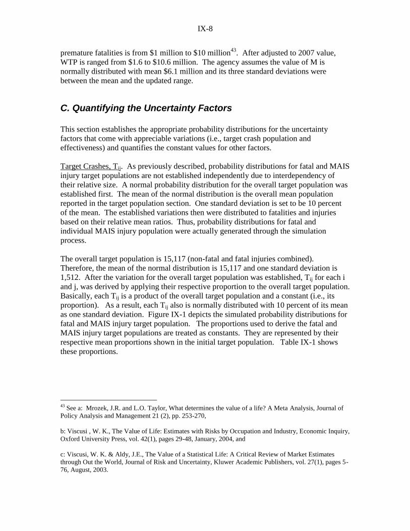
IX-8

premature fatalities is from $1 million to $10 million43

. After adjusted to 2007 value,

WTP is ranged from $1.6 to $10.6 million. The agency assumes the value of M is

normally distributed with mean $6.1 million and its three standard deviations were

between the mean and the updated range.

C. Quantifying the Uncertainty Factors

This section establishes the appropriate probability distributions for the uncertainty

factors that come with appreciable variations (i.e., target crash population and

effectiveness) and quantifies the constant values for other factors.

Target Crashes, Tij. As previously described, probability distributions for fatal and MAIS

injury target populations are not established independently due to interdependency of

their relative size. A normal probability distribution for the overall target population was

established first. The mean of the normal distribution is the overall mean population

reported in the target population section. One standard deviation is set to be 10 percent

of the mean. The established variations then were distributed to fatalities and injuries

based on their relative mean ratios. Thus, probability distributions for fatal and

individual MAIS injury population were actually generated through the simulation

process.

The overall target population is 15,117 (non-fatal and fatal injuries combined).

Therefore, the mean of the normal distribution is 15,117 and one standard deviation is

1,512. After the variation for the overall target population was established, Tij for each i

and j, was derived by applying their respective proportion to the overall target population.

Basically, each Tij is a product of the overall target population and a constant (i.e., its

proportion). As a result, each Tij also is normally distributed with 10 percent of its mean

as one standard deviation. Figure IX-1 depicts the simulated probability distributions for

fatal and MAIS injury target population. The proportions used to derive the fatal and

MAIS injury target populations are treated as constants. They are represented by their

respective mean proportions shown in the initial target population. Table IX-1 shows

these proportions.

43

See a: Mrozek, J.R. and L.O. Taylor, What determines the value of a life? A Meta Analysis, Journal of

Policy Analysis and Management 21 (2), pp. 253-270,

b: Viscusi , W. K., The Value of Life: Estimates with Risks by Occupation and Industry, Economic Inquiry,

Oxford University Press, vol. 42(1), pages 29-48, January, 2004, and

c: Viscusi, W. K. & Aldy, J.E., The Value of a Statistical Life: A Critical Review of Market Estimates

through Out the World, Journal of Risk and Uncertainty, Kluwer Academic Publishers, vol. 27(1), pages 5-

76, August, 2003.

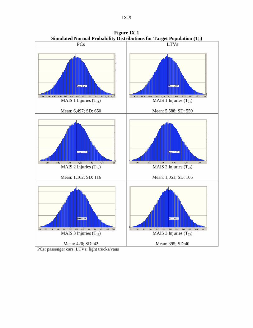
IX-9

Figure IX-1

Simulated Normal Probability Distributions for Target Population (Tij)

PCs LTVs

MAIS 1 Injuries (T11)

Mean: 6,497; SD: 650

MAIS 1 Injuries (T21)

Mean: 5,588; SD: 559

MAIS 2 Injuries (T12)

Mean: 1,162; SD: 116

MAIS 2 Injuries (T22)

Mean: 1,051; SD: 105

MAIS 3 Injuries (T13)

Mean: 420; SD: 42

MAIS 3 Injuries (T23)

Mean: 395; SD:40 PCs: passenger cars, LTVs: light trucks/vans

IX-10

Figure IX-1 - Continued

Simulated Normal Probability Distributions for Target Population (Tij)

MAIS 4 Injuries (T14)

Mean: 60; SD: 6

MAIS 4 Injuries (T24)

Mean: 57; SD: 6

MAIS 5 Injuries (T15)

Mean: 29; SD: 3

MAIS 5 Injuries (T25)

Mean: 28; SD: 3

Fatalities (T16)

Mean: 59; SD: 6

Fatalities (T26)

Mean: 169; SD: 17

PCs: passenger cars, LTVs: light trucks/vans

IX-11

Table IX-1

Constant Values for Distributing Target Population

PCs LTVs

MAIS 1 0.4187 0.3602

MAIS 2 0.0749 0.0677

MAIS 3 0.0271 0.0255

MAIS 4 0.0039 0.0037

MAIS 5 0.0019 0.0018

Fatalities 0.0038 0.0109

Column Total 0.5302 0.4698

Avoidability fA.. Values of fA are assumed to be beta distributed and bounded by the

percentage of avoidable cases and the combined percentage of “avoidable”, “possibly

avoidable”, and “possibly not avoidable” cases. The shape parameters α and β of the

beta distribution function were determined by ensuring that the mean of the distribution is

equal to the percentage of avoidable and possible avoidable cases. Figure IX-2 depicts

the beta distribution for each of the technologies examined in the PRIA. Due to the range

and mean constraints, as shown, these distributions tend to be negatively skewed, i.e., a

distribution with a relatively longer tail towards the lower end of values.

System performance factor, fS. The system performance factor represents the average

performance of sensors. Thus, it only impacts sensor-based ultrasonic and radar systems.

Its effect on these two systems is assumed to be identical. Values of fS are treated as

uniformly distributed. Since the factor does not apply to the camera systems, it is set to

be 1.

Two parameters maximum (fSMax) and minimum (fSMin) are required to establish a

uniform distribution for fs. With these two parameters, the uniform distribution can be

represented as:

The mean of the distribution is set to be the point estimate presented in the previous

chapter. The maximum and minimum of fs are assumed to be a 10 percent deviation from

the mean, i.e., 0.9*mean ≤ fs ≤ 1.1*mean. Therefore, for ultrasonic and radar systems,

the mean of fs is 70.37 percent, fSMin = 63.33 percent, and fSMax = 77.41 percent.

IX-12

Figure IX-2

Beta Distributions for Avoidability Factor (fA)

by Technology

180

o View Camera

Minimum: 66%; Maximum: 94%

Mean: 90%

α = 11; β = 2

130

o View Camera

Minimum: 50%; Maximum: 86%

Mean: 76%

α = 5.5; β = 2

Ultrasonic

Minimum: 20%; Maximum: 68%

Mean: 49%

α = 3; β = 2

Radar

Minimum: 24%; Maximum: 74%

Mean: 54%

α = 3; β = 2

Driver factor, fDR. This factor varies depending on whether the technology of interest is a

camera- or sensor-based system. Values for this factor are assumed to be normally

distributed for both systems. One standard deviation is set to be the 10 percent of the

mean. Figure IX-3 depicts the normal distribution for fDR.

IX-13

Figure IX-3

Normal Distribution for Driver Factor (fDR)

Camera Systems

(180o and 130

o View)

Mean: 55%; SD: 6%

Sensor-Based Systems

(Ultrasonic and Radar)

Mean: 7%; SD: 1%

2010-based adjustment factors, aij. The analysis treats these factors as constant. They

vary by vehicle types (i.e., PCs and LTVs) and technology types. Table IX-2 lists these

constants. As shown, for camera systems, a11 = 82.2%, a12 = 7.3%, a21 = 56.7%, and a22

= 13.2%. For sensor-based systems, a11 = 90.9%, a12 = 0.0%, a21 = 70.3%, and a22 =

0.0%. Note that the factor ai used in the FE model is the sum of full and partial system

factors as shown in the table. For example, a1 = 89.5% and a2 = 69.9% for camera

systems and a1 = 90.9% and a2 = 70.3% for sensor-based systems.

IX-14

Table IX-2

Constant Values for 2010-Based Adjustment Factors (aij) by Technology and

Vehicle Type

Detection Technology PCs LTVs

Camera Systems

(180o and 130

o View)

Full System

Partial System*

Total

82.2%

7.3%

89.5%

56.7%

13.2%

69.9%

Sensor-Based Systems

(Ultrasonic and Radar)

Full System

Partial System*

Total

90.9%

0.0%

90.9%

70.3%

0.0%

70.3%

*Needed only the camera, only applicable to camera-based systems

Injury-to-fatality equivalent ratios (ri). These factors are treated as constants. Table IX-3

lists the injury-to-fatality equivalent ratios which are used to translate non-fatal injuries to

fatal equivalents.

Table IX-3

Injury-To-Fatality Equivalence Ratios (rj)*

Injury-To-Fatality Equivalence Ratios

MAIS 1 (r1) 0.00275

MAIS 2 (r2) 0.04356

MAIS 3 (r3) 0.08037

MAIS 4 (r4) 0.19981

MAIS 5 (r5) 0.66558

Fatality (r6) 1.00000

Cumulative lifetime discount factors (di). These factors are treated as constants. At a 3

percent discount, d1 = 0.8304 for PCs and d2 = 0.8022 for LTVs. At 7 percent discount,

d1 = 0.6700 for PCs and d2 = 0.6303 for LTVs.

Unit lifetime property damage savings, ui. The analysis treats these factors as uniformly

distributed. Table IX-4 lists the maximum and minimum values that are used to

establish the uniform distribution. The mean values are also presented in the table. Note

that negative values represent cost. As shown, both cameras systems would save

property damage costs at both discount rates. In contrast, the ultrasonic and radar

systems would not.

IX-15

Table IX-4

Discounted Unit Lifetime Property Damage Savings Per Vehicle (ui)

Parameters for Uniform Distribution by Technology Type and Discount Rate

(2007 Dollar)

@3% Discount Mean Minimum Maximum

180o View Camera $28.56 $25.70 $31.42

130o View Camera $31.43 $28.29 $34.57

Ultrasonic -$3.35 -$3.69 $-3.02

Radar -$5.50 -$6.05 -$4.95

@7% Discount Mean Minimum Maximum

180o View Camera $23.59 $21.23 $25.95

130o View Camera $25.96 $23.36 $28.56

Ultrasonic -$2.76 -$3.04 $-2.48

Radar -$4.54 -$4.99 -$4.09

Note: negative numbers represent cost

Technology cost per affected vehicle, ci. The analysis assumes the cost factors are

uniformly distributed. As described earlier, a uniform distribution would be established

by a maximum and a minimum value. Based on expert judgment and the agency‟s

experience with cost assessment, a 10 percent cost fluctuation from the mean cost is

believed to be sufficient to describe the overall technology cost variation. The cost varies

by technology and its installation options. Table IX-5 lists the cost per affected vehicle

by technology and installation options. These costs represent the investments paid now

for future benefits and thus no discounting is needed.

IX-16

Table IX-5

Parameters for Uniform Distribution for Technology Cost per Affected Vehicle (ci)

by Technology Type and Installation Option

(2007 Dollar) Technology – Installation Mean Minimum Maximum

180o View Camera – Mirror $202.94 $182.65 $223.24

130o View Camera – Mirror $172.74 $155.47 $190.02

180o View Camera – Dashboard

Full System

Camera Only (Partial System)

$189.05

$88.18

$170.15

$79.37

$207.96

$97.00

130o View Camera – Dashboard

Full System

Camera Only (Partial System)

$158.85

$57.98

$142.97

$52.19

$174.74

$63.78

Ultrasonic $51.49 $46.34 $56.64

Radar $92.26 $83.03 $101.49

Number of new vehicles, vi,. These factors are constant. The total number of passenger

vehicles is 16.6 million. Of these, 8,000,000 are PCs, and 8,600,000 are LTVs. In other

words, v1 = 8,000,000 and v2 = 8,600,000

Cost per fatality, M, is an uncertainty factor for net benefits. The value of M largely

depends on the value of statistical life (VSL). The cost is based on recent meta-analyses

of the wage-risk value of VSL. These meta-analyses deployed different statistical

methodologies and assumptions. But, generally, these studies show that an individual‟s

willingness-to-pay (WTP) for reduction in premature fatalities is from $1 million to $10

million44

. In the past, when a $3.0 million VSL was the DOT guideline for cost-benefit

analysis, the agency used this $1-$10 million as the range for M and assumed the value of

M is normally distributed with its mean equal to $5.5.million. However, in 2008 DOT

has issued a new guideline requiring a $5.8 million VSL to be used for cost-benefit

analysis. The corresponding comprehensive cost is estimated to be $6.1 million in 2007

dollars. To reflect this change and to be consistent with the cost-benefit analysis

described in the previous chapters, the normal distribution for M has been revised to

reflect the comprehensive cost per fatality. Thus, the distribution for M has a mean of

44 See a: Mrozek, J.R. and L.O. Taylor, What determines the value of a life? A Meta

Analysis, Journal of Policy Analysis and Management 21 (2), pp. 253-270, b: Viscusi , W. K., The Value of Life: Estimates with Risks by Occupation and Industry, Economic Inquiry,

Oxford University Press, vol. 42(1), pages 29-48, January, 2004, and

c: Viscusi, W. K. & Aldy, J.E., The Value of a Statistical Life: A Critical Review of Market Estimates

through Out the World, Journal of Risk and Uncertainty, Kluwer Academic Publishers, vol. 27(1), pages 5-

76, August, 2003.

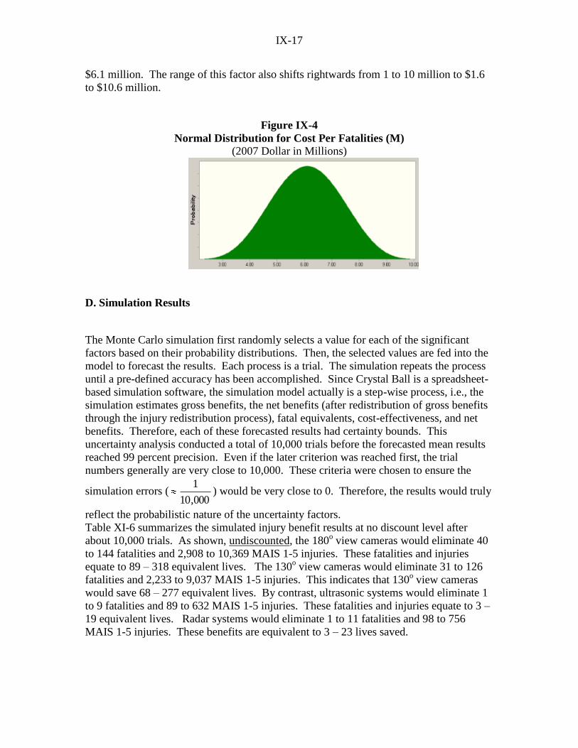
IX-17

$6.1 million. The range of this factor also shifts rightwards from 1 to 10 million to $1.6

to $10.6 million.

Figure IX-4

Normal Distribution for Cost Per Fatalities (M)

(2007 Dollar in Millions)

D. Simulation Results

The Monte Carlo simulation first randomly selects a value for each of the significant

factors based on their probability distributions. Then, the selected values are fed into the

model to forecast the results. Each process is a trial. The simulation repeats the process

until a pre-defined accuracy has been accomplished. Since Crystal Ball is a spreadsheet-

based simulation software, the simulation model actually is a step-wise process, i.e., the

simulation estimates gross benefits, the net benefits (after redistribution of gross benefits

through the injury redistribution process), fatal equivalents, cost-effectiveness, and net

benefits. Therefore, each of these forecasted results had certainty bounds. This

uncertainty analysis conducted a total of 10,000 trials before the forecasted mean results

reached 99 percent precision. Even if the later criterion was reached first, the trial

numbers generally are very close to 10,000. These criteria were chosen to ensure the

simulation errors (000,10

1) would be very close to 0. Therefore, the results would truly

reflect the probabilistic nature of the uncertainty factors.

Table XI-6 summarizes the simulated injury benefit results at no discount level after

about 10,000 trials. As shown, undiscounted, the 180o view cameras would eliminate 40

to 144 fatalities and 2,908 to 10,369 MAIS 1-5 injuries. These fatalities and injuries

equate to 89 – 318 equivalent lives. The 130o view cameras would eliminate 31 to 126

fatalities and 2,233 to 9,037 MAIS 1-5 injuries. This indicates that 130o view cameras

would save 68 – 277 equivalent lives. By contrast, ultrasonic systems would eliminate 1

to 9 fatalities and 89 to 632 MAIS 1-5 injuries. These fatalities and injuries equate to 3 –

19 equivalent lives. Radar systems would eliminate 1 to 11 fatalities and 98 to 756

MAIS 1-5 injuries. These benefits are equivalent to 3 – 23 lives saved.

IX-18

Table IX-6

Simulated Injury Benefits (No Discount)

180o View

Camera

130o View

Camera

Ultrasonic Radar

Fatalities Reduced

Mean 84 71 4 5

Range 40 – 144 31 – 126 1 – 9 1 – 11

90% Certainty 64 – 104 53 – 90 3 – 6 3 – 7

MAIS Injuries Eliminated

Mean 5,998 5,107 299 331

Range 2,908 – 10,369 2,233 – 9,037 89 – 632 98 – 756

90% Certainty 4,626 – 7,480 3,831 – 6,500 181 – 428 205 – 469

Equivalent Lives Saved

Mean 184 157 9 10

Range 89 – 318 68 – 277 3 – 19 3 – 23

90% Certainty 142 – 229 117 – 199 6 – 13 6 – 14

Tables IX-7 and IX-8 summarize the simulated cost-effectiveness and net benefit results

at 3 and 7 percent discount, respectively. As shown in Table IX-7, at a 3 percent discount

rate, the 180o view camera systems would save 116 - 187 equivalent lives with a 90

percent certainty. With the same level of certainty, the 130o view camera systems would

save 96 - 162 equivalent lives, the ultrasonic systems would save 5 - 11 equivalent lives,

and the radar systems would save 5 - 12 equivalent lives.

With the same 90 percent certainty, the net cost would range from $1.7 (dashboard

systems) to $2.5 billion (mirror systems) for the 180o view camera systems, $1.3 to $2.1

billion for the 130o view camera systems, $0.7 to $0.8 billion for the ultrasonic systems,

and $1.2 to $1.4 billion for the radar systems.

At a 7 percent discount rate, as shown in Table IX-8, the 180o view camera systems

would save 92 - 149 equivalent lives with a 90 percent certainty. At this certainty level,

the 130o view camera systems would save 76 - 129 equivalent lives. Both ultrasonic and

radar systems each would save 4 - 9 equivalent lives.

The net cost would range from $1.8 to $2.6 billion for the 180o view camera systems,

$1.4 to $2.1 billion for the 130o view camera systems, $0.7 to $0.9 billion for the

ultrasonic systems, and $1.2 to $1.4 billion for the radar systems (cost ranges are similar

to those at 3% discount rate due to rounding).

IX-19

All four technologies examined in the PRIA are not cost effective based on the $6.1

million per fatality and $0 net benefit measurements. At both discount rates, none of the

four technologies would have chance to produce a cost per equivalent fatality of no more

than $6.1 million. Also, none of these technologies would generate a positive net benefit.

IX-20

Table IX-7

Simulated Cost-Effectiveness and Net Benefits

(2007 Dollar)

@3% Discount Camera Systems

Technology Costs* 180

o View

Mirror

130o View

Mirror

180o View

Dashboard

130o View

Dashboard

Mean $2,673 M $2,276 M $2,317 M $1,919 M

Total Range $2,406 – $2,940 M $2,048 – $2,503 M $2,085 – $2,548 M $1,728 – $2,111 M

90% Certainty Range $2,433 – $2,914 M $2,070 – $2,480 M $2,122 – $2,512 M $1,756 – $2,083 M

Equivalent Lives Saved

Mean 150 128 150 128

Total Range 73 – 259 56 – 226 73 – 259 56 – 226

90% Certainty Range 116 – 187 96 – 162 116 – 187 96 – 162

Lifetime Property Damage

Savings

Mean $376 M $414 M $376 M $414 M

Total Range $339 – $414 M $373 – $455 M $339 – $414 M $373 – $455 M

90% Certainty Range $342 – $410 M $377 – $451 M $342 – $410 M $377 – $451 M

Net Cost**

Mean $2,297 M $1,862 M $1,941 M $1,505 M

Total Range $1,993 – $2,600 M $1,593 – $2,130 M $1,678 – $2,208 M $1,275 – $1,737 M

90% Certainty Range $2,056 – $2,539 M $1,654 – $2,069 M $1,743 – $2,138 M $1,336 – $1,674 M

Lifetime Property Damage Cost

Cost-Effectiveness (CE)

Mean $15.7 M $15.0 M $13.2 M $12.1 M

Total Range $8.2 – $33.1 M $7.6 – $36.4 M $6.8 – $27.2 M $6.0 – $29.4 M

90% Certainty Range $11.9 – $20.3 M $11.1 – $19.9 M $10.1 – $17.2 M $9.0 – $16.1 M

Certainty that CE ≤ $6.1 M 0% 0% 0% 0%

Net Benefit (NB)

Mean -$1,383 M -$1,083 M $-1,029 M $-727 M

Total Range -$2,248 to -$93 M -$1,873 to $21 M -$1,874 to $359 M -$1,457 to $420 M

90% Certainty Range -$1,825 to -$909 M -$1,469 to -$667 M -$1,441 to -$578M -$1,086 to -$333M

Certainty that NB > $0 0% 0% 0% 0.2%

M: million

* No discount required, same for all discount rates

** = Technology Cost – Lifetime Property Damage Savings

IX-21

Table IX-7 - Continued

Simulated Cost-Effectiveness and Net Benefits

(2007 Dollar)

@3% Discount Sensor Systems

Technology Costs* Ultrasonic Radar

Mean $686 M $1,229 M

Total Range $617 – $754 $1,106 – $1,352

90% Certainty Range $524 – $747 $1,118 – $1,339

Equivalent Lives Saved

Mean 7 8

Total Range 2 – 16 2 – 19

90% Certainty Range 5 – 11 5 – 12

Lifetime Property Damage Savings

Mean -$45 M -$73 M

Total Range -$49 to -$40 M -$81 to -$66 M

90% Certainty Range -$49 to -$41 M -$80 to -$67 M

Net Cost**

Mean $731 M $1,302 M

Total Range $657 – $803 M $1,172 – $1,432 M

90% Certainty Range $669 – $792 M $1,191 – $1,413 M

Cost-Effectiveness (CE)

Mean $104.8 M $168.0 M

Total Range $44.1 – $349.3 M $63.1 – $574.0 M

90% Certainty Range $67.5 – $162.7 M $109.8 – $255.5 M

Certainty that CE ≤ $6.1 M 0% 0%

Net Benefit (NB)

Mean -$585 M -$1,252 M

Total Range -$786 to -$555 M -$1,410 to -$1,063 M

90% Certainty Range -$752 to -$618 M -$1,366 to -$1,139 M

Certainty that NB > $0 0% 0%

M: million

* No discount required, same for all discount rates

** = Technology Cost – Lifetime Property Damage Savings

IX-22

Table IX-8

Simulated Cost-Effectiveness and Net Benefits

(2007 Dollar)

@7% Discount Camera Systems

Technology Costs* 180

o View

Mirror

130o View

Mirror

180o View

Dashboard

130o View

Dashboard

Mean $2,673 M $2,276 M $2,317 M $1,919 M

Total Range $2,406 – $2,940 M $2,048 – $2,503 M $2,085 – $2,548 M $1,728 – $2,111 M

90% Certainty Range $2,433 – $2,914 M $2,070 – $2,480 M $2,122 – $2,512 M $1,756 – $2,083 M

Equivalent Lives Saved

Mean 119 102 119 102

Total Range 58 – 206 44 – 180 58 – 206 44 – 180

90% Certainty Range 92 – 149 76 – 129 92 – 149 76 – 129

Lifetime Property Damage

Savings

Mean $311 M $342 M $311 M $342 M

Total Range $280 – $342 M $308 – $376 M $280 – $342 M $308 – $376 M

90% Certainty Range $283 – $339 M $311 – $373 M $283 – $339 M $311 – $373 M

Net Cost**

Mean $2,363 M $1,934 M $2,006 M $1,577 M

Total Range $2,065 – $2,660 M $1,672 – $2,194 M $1,750 – $2,266 M $1,354 – $1,800 M

90% Certainty Range $2,122 – $2,603 M $1,727 – $2,140 M $1,810 – $2,203 M $1,411 – $1,744 M

Cost-Effectiveness (CE)

Mean $20.2 M $19.6 M $17.2 M $15.9 M

Total Range $10.8 – $43.3 M $9.9 – $47.5 M $9.0 – $35.2 M $7.8 – $38.7 M

90% Certainty Range $15.5 – $26.2 M $14.6 – $25.9 M $13.2 – $22.0 M $11.9 – $21.1 M

Certainty that CE ≤ $6.1 M 0% 0% 0% 0%

Net Benefit (NB)

Mean -$1,635 M -$1,314 M -$1,279 M $-958 M

Total Range -$2,397 to -$607 M -$1,955 to -$391 M -$1,983 to -$155 M -$1,559 to -$29 M

90% Certainty Range -$2,020 to -$1,231 M -$1,648 to -$960 M -$1,634 to -$902 M -$1,264 to -$628 M

Certainty that NB > $0 0% 0% 0% 0%

M: million

* No discount required, same for all discount rates

** = Technology Cost – Lifetime Property Damage Savings

IX-23

Table IX-8 - Continued

Simulated Cost-Effectiveness and Net Benefits

(2007 Dollar)

@7% Discount Sensor Systems

Technology Costs* Ultrasonic Radar

Mean $686 M $1,229 M

Total Range $617 – $754 $1,106 – $1,352

90% Certainty Range $524 – $747 $1,118 – $1,339

Equivalent Lives Saved

Mean 6 7

Total Range 2 – 13 2 – 15

90% Certainty Range 4 – 9 4 – 9

Lifetime Property Damage Savings

Mean -$37 M -$60 M

Total Range -$40 to -$33 M -$67 to -$54 M

90% Certainty Range -$40 to -$33 M -$66 to -$55 M

Net Cost**

Mean $723 M $1,289 M

Total Range $651 – $795 M $1,161 – $1,418 M

90% Certainty Range $661 – $784 M $1,179 – $1,400 M

Cost-Effectiveness (CE)

Mean $130.3 M $209.1 M

Total Range $54.8 – $435.6 M $78.6 – $718.8 M

90% Certainty Range $83.9 – $202.3 M $136.7 – $318.0 M

Certainty that CE ≤ $6.1 M 0% 0%

Net Benefit (NB)

Mean -$686 M -$1,249 M

Total Range -$782 to -$568 M -$1,401 to -$1,068 M

90% Certainty Range -$751 to -$622 M -$1,362 to -$1,137 M

Certainty that NB > $0 0% 0%

M: million

* No discount required, same for all discount rates

** = Technology Cost – Lifetime Property Damage Savings

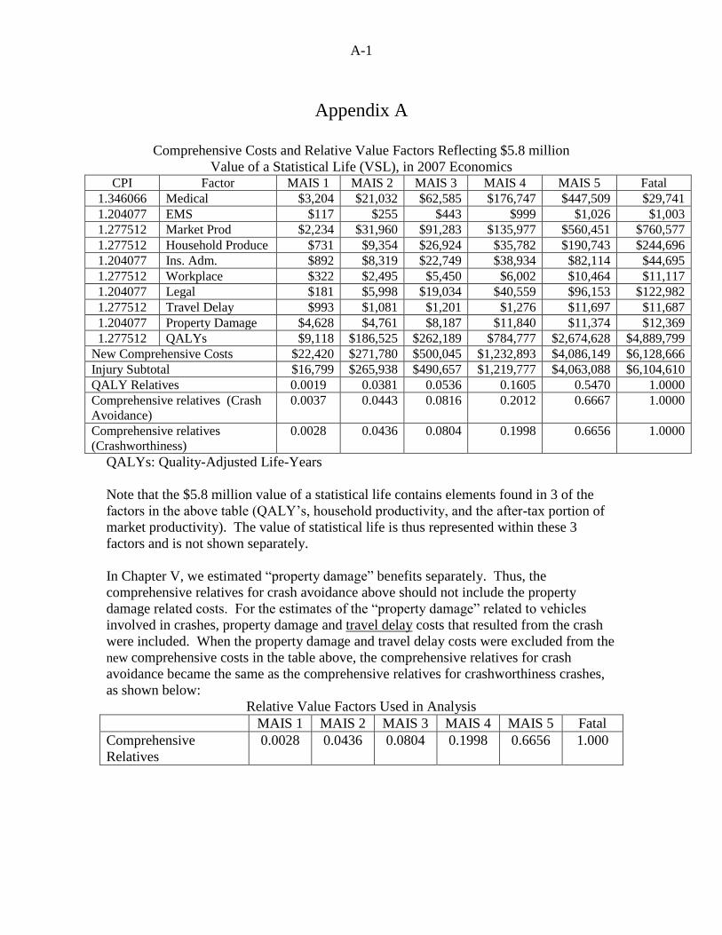
A-1

Appendix A

Comprehensive Costs and Relative Value Factors Reflecting $5.8 million

Value of a Statistical Life (VSL), in 2007 Economics CPI Factor MAIS 1 MAIS 2 MAIS 3 MAIS 4 MAIS 5 Fatal

1.346066 Medical $3,204 $21,032 $62,585 $176,747 $447,509 $29,741

1.204077 EMS $117 $255 $443 $999 $1,026 $1,003

1.277512 Market Prod $2,234 $31,960 $91,283 $135,977 $560,451 $760,577

1.277512 Household Produce $731 $9,354 $26,924 $35,782 $190,743 $244,696

1.204077 Ins. Adm. $892 $8,319 $22,749 $38,934 $82,114 $44,695

1.277512 Workplace $322 $2,495 $5,450 $6,002 $10,464 $11,117

1.204077 Legal $181 $5,998 $19,034 $40,559 $96,153 $122,982

1.277512 Travel Delay $993 $1,081 $1,201 $1,276 $11,697 $11,687

1.204077 Property Damage $4,628 $4,761 $8,187 $11,840 $11,374 $12,369

1.277512 QALYs $9,118 $186,525 $262,189 $784,777 $2,674,628 $4,889,799

New Comprehensive Costs $22,420 $271,780 $500,045 $1,232,893 $4,086,149 $6,128,666

Injury Subtotal $16,799 $265,938 $490,657 $1,219,777 $4,063,088 $6,104,610

QALY Relatives 0.0019 0.0381 0.0536 0.1605 0.5470 1.0000

Comprehensive relatives (Crash

Avoidance)

0.0037 0.0443 0.0816 0.2012 0.6667 1.0000

Comprehensive relatives

(Crashworthiness)

0.0028 0.0436 0.0804 0.1998 0.6656 1.0000

QALYs: Quality-Adjusted Life-Years

Note that the $5.8 million value of a statistical life contains elements found in 3 of the

factors in the above table (QALY‟s, household productivity, and the after-tax portion of

market productivity). The value of statistical life is thus represented within these 3

factors and is not shown separately.

In Chapter V, we estimated “property damage” benefits separately. Thus, the

comprehensive relatives for crash avoidance above should not include the property

damage related costs. For the estimates of the “property damage” related to vehicles

involved in crashes, property damage and travel delay costs that resulted from the crash

were included. When the property damage and travel delay costs were excluded from the

new comprehensive costs in the table above, the comprehensive relatives for crash

avoidance became the same as the comprehensive relatives for crashworthiness crashes,

as shown below:

Relative Value Factors Used in Analysis

MAIS 1 MAIS 2 MAIS 3 MAIS 4 MAIS 5 Fatal

Comprehensive

Relatives

0.0028 0.0436 0.0804 0.1998 0.6656 1.000

B-1

Appendix B

Year/Make/Model Vehicle Type

Laser BZ50x

50

Laser BZ50x

20

Laser BZ50x

8

Laser BZ50x

6

Laser Sight Dist

Backing

Risk

2008 Mazda Mazda6 4-door Car 932 376 164 123 21.0 1.5

2008 Hyundai Accent 4-door Car 938 391 198 141 25.3

2003 Nissan Sentra 4-door Car 974 344 154 104 17.4 1.6

2008 Hyundai Azera 4-door Car 1167 494 233 173 29.6

2008 Nissan Versa 5-door Car 1184 435 144 99 17.4

2005 Volkswagen Jetta 4-door Car 1227 666 249 179 31.6 1.6

2008 Dodge Caliber 4-door Car 1253 652 249 159 31.6

2009 Hyundai Sonata 4-door Car 1299 631 281 207 29.4

2007 Chevrolet Monte Carlo 2-door Car 1300 479 175 136 22.4 2.1

2008 Volkswagen New GTI 3-door Car 1332 441 154 109 19.8

2007 Ford Five Hundred 4-door Car 1372 651 235 170 29.9 2

2008 Honda Fit 5-door Car 1384 491 161 101 20.3

2008 Volkswagen New Beetle 3-door Car 1388 477 155 100 13.8 1.4

2008 Volvo S80 4-door Car 1393 604 229 152 29.1

2008 Toyota Prius 5-door Car 1415 642 257 191 12.1 1.9

2008 Pontiac G6 4-door Car 1436 733 313 226 39.5 1.6

2008 Ford Focus 4-door Car 1489 726 289 216 36.6

2008 Honda Accord 4-door Car 1499 742 264 174 33.5

2008 Mazda Mazda3 4-door Car 1545 689 285 200 36.1 1.9

2006 BMW 3-Series 4-door Car 1546 788 318 232 40.0

2009 Acura RL 4-door Car 1547 641 271 202 34.4

2008 Dodge Charger 4-door Car 1552 755 283 199 35.9

2008 Kia Spectra 4-door Car 1558 710 255 169 26.1

2005 Saturn Ion 4-door Car 1561 863 380 290 47.9 1.1

2008 BMW 5-Series 4-door Car 1584 756 234 156 29.8

2005 Chrysler 300 4-door Car 1619 816 303 228 38.3 2.3

2008 Buick Lucerne 4-door Car 1620 792 325 240 41.0

2008 Infiniti EX35 Stationwagon Car 1668 641 274 202 34.5

2008 Hyundai Elantra 4-door Car 1676 755 270 192 28.1

2008 Volkswagen Jetta 4-door Car 1681 803 301 207 31.9

2008 Chevrolet Aveo 4-door Car 1685 671 255 182 32.3

2009 Subaru Legacy 4-door Car 1689 866 344 250 37.2

2006 Volkswagen Passat 4-door Car 1693 852 339 257 42.8

2008 Toyota Avalon 4-door Car 1704 819 298 198 37.6

2005 Cadillac STS 4-door Car 1753 891 366 266 45.9

2008 Ford Fusion 4-door Car 1825 878 363 273 39.5

2007 Lexus ES 4-door Car 1848 867 370 270 40.3

2009 Toyota Corolla Matrix 5-door Car 1848 875 360 260 40.1

2008 Dodge Dakota Quad Cab Pickup 1508 606 201 139 25.6 4.6

2007 Chevrolet 1500 Silverado Crew Cab

Pickup 1586 767 311 235 39.4

2008 Honda Ridgeline Pickup 1662 652 255 200 30.8

2008 GMC 1500 Sierra Regular Cab Short Bed

Pickup 1664 729 345 259 43.6

2008 Ford F-150 Super Cab Long Pickup 1804 939 395 297 49.3

B-2

Bed

2005 Honda CR-V SUV 1217 545 191 140 24.4 3.1

2008 Chevrolet Trailblazer SUV 1268 602 239 158 30.3 3.1

2005 Ford Explorer SUV 1284 435 157 121 19.0 3

2008 Jeep Wrangler SUV 1323 679 302 216 38.1

2008 Hyundai Santa Fe SUV 1350 528 206 141 26.3

2007 Dodge Magnum SUV 1369 619 218 155 27.8 2

2008 Kia Sportage SUV 1408 639 266 191 33.8

2008 Jeep Grand Cherokee SUV 1411 674 248 178 31.5 3.4

2009 Chevrolet HHR SUV 1475 715 274 194 34.6

2008 Toyota RAV4 SUV 1516 713 279 204 28.0

2008 Toyota 4Runner SUV 1518 655 201 128 25.6 4.1

2008 Honda CR-V SUV 1538 595 217 161 27.6

2007 Suzuki Grand Vitara SUV 1547 760 252 161 31.3

2006 Honda Pilot SUV 1594 775 290 190 36.6 3.3

2008 Saturn Vue SUV 1625 839 337 243 42.4

2008 Scion xB SUV 1625 820 298 211 37.5

2008 Ford Edge SUV 1648 866 327 227 41.1

2008 Ford Expedition EL SUV 1664 698 280 201 35.5

2008 Chevrolet 1500 Suburban SUV 1778 838 374 274 46.9

2007 Jeep Commander SUV 1792 941 400 300 50.0 4

2008 Chevrolet Equinox SUV 1805 877 387 294 48.5 2.9

2008 Ford Taurus X SUV 1814 843 349 249 41.3 2.3

2008 Subaru Tribeca SUV 1842 943 400 300 50.0

2008 Mazda CX-9 SUV 1880 873 365 272 40.4

2007 Cadillac Escalade SUV 1890 843 352 261 44.3

2008 Saturn Outlook SUV 1955 956 400 300 50.0

2008 Chevrolet 1500 Avalanche SUV 2010 923 387 290 48.8

2008 Dodge Caravan Wagon Van 1174 595 200 139 25.5

2006 Chrysler PT Cruiser Wagon Van 1265 573 215 140 24.0

2005 Chevrolet Uplander Wagon Van 1442 796 333 246 41.9 3.2

2007 Honda Odyssey Wagon Van 1812 874 335 235 42.1 5.1

2008 Ford E-250 Cargo Van 2500 1000 400 300 50.0 5.3