autonomous trading and investing - worcester polytechnic institute
TRANSCRIPT

WORCESTER POLYTECHNIC INSTITUTE
Autonomous Trading and Investing
Interactive Qualifying Project Report
Jason Howell Walter McIntyre
Vinnie McMahon
5/26/2013

2
Contents Abstract ......................................................................................................................................................... 5
Introduction .................................................................................................................................................. 6
The Importance of Investing and Saving ................................................................................................... 6
Investing in the Modern Day..................................................................................................................... 6
Background ................................................................................................................................................... 7
Characteristics of Different Trading Styles ............................................................................................... 7
Trading Markets ........................................................................................................................................ 8
The News ................................................................................................................................................... 9
Understanding Monetary Policy ............................................................................................................... 9
Intermarket Analysis ............................................................................................................................... 11
Sectors in the Stock Market .................................................................................................................... 13
Industry Groups ...................................................................................................................................... 15
Sector Rotation ....................................................................................................................................... 15
Stock Market Indices ............................................................................................................................... 17
Trading System Development ................................................................................................................. 18
Manual and Automated Trading Styles .................................................................................................. 18
Basic Strategy Techniques ...................................................................................................................... 19
Advanced Strategy Techniques ............................................................................................................... 20
Expectancy and Profitability ............................................................................................................... 20
Position Sizing ..................................................................................................................................... 21
Exploiting the Majority........................................................................................................................ 21
Entry and Exit Rules ................................................................................................................................ 22
Trading Indicators ................................................................................................................................... 23
Support and Resistance ...................................................................................................................... 23
Trend Lines .......................................................................................................................................... 24
Moving Averages ................................................................................................................................. 24
The multiplier (weight) allows it so that more recent data is taken to be more important than past
data. In Figure 10, the differences between simple and exponential moving average can be seen
visually.9 .................................................................................................................................................. 25
Bollinger Bands ................................................................................................................................... 26
Average True Range ............................................................................................................................ 26

3
Precision Trading System .................................................................................................................... 27
Chandelier Exit .................................................................................................................................... 28
Yo-Yo Exit ............................................................................................................................................ 28
Modified Parabolic Exit ....................................................................................................................... 29
Stock Screening ....................................................................................................................................... 30
Back-Testing and Optimization ............................................................................................................... 32
Methodology ............................................................................................................................................... 33
Jason Howell’s Trading Strategy ............................................................................................................. 33
Problems with Two Line EMA System and Attempted Solutions ....................................................... 34
Entry Rules .......................................................................................................................................... 34
Exit Rules ............................................................................................................................................. 36
Position Sizing ..................................................................................................................................... 37
Ben McIntyre’s PTS Strategies ................................................................................................................ 38
PTSmulti Objectives ............................................................................................................................ 39
PTSrocket Objectives .......................................................................................................................... 42
PTStrending Objectives ....................................................................................................................... 45
System Part 3: by Vinnie McMahon ........................................................................................................ 47
Exit Types: Which is best suited for stocks? ....................................................................................... 52
Results ......................................................................................................................................................... 54
Results of Jason Howell’s Strategy .......................................................................................................... 54
Results of Vinnie McMahon’s Strategy ................................................................................................... 57
Results of Ben McIntyre’s PTS Strategies ................................................................................................ 60
Expectancy, Expectunity, and System Quality .................................................................................... 60
Optimization Results ........................................................................................................................... 61
Strategy Performance Reports ............................................................................................................ 64
Performance Charts ............................................................................................................................ 65
PTSrocket Performance Chart ............................................................................................................. 68
Walk-Forward Analysis ........................................................................................................................ 70
Conclusion and Future Work ...................................................................................................................... 73
Jason Howell’s EMA Strategy .................................................................................................................. 73
Vince McMahon’s System ....................................................................................................................... 73
Ben McIntyre’s PTS Strategies ................................................................................................................ 74

4
References .................................................................................................................................................. 74
Appendix A: Jason’s Code ........................................................................................................................... 76
Appendix B: Ben’s Code .............................................................................................................................. 82
PTSmulti code ......................................................................................................................................... 82
PTStrending Code .................................................................................................................................... 84
PTSrocket Code ....................................................................................................................................... 87

5
Abstract Trading is a course of action that was created thousands of years ago as a means to survive.
Modern day trading now relates to investing into companies and is now much more extensive.
Computers have allowed nearly instant trading from across the world so that the trader can make profit
from their home. Computers also allow completely autonomous trading that a person can just watch
make profit while they do other things throughout their day. Throughout this paper, a lot of different
trading techniques and strategies are addressed including Lebau’s exits, PTS strategies, and more.

6
Introduction
The Importance of Investing and Saving
People invest for so many different reasons. Some do it for enjoyment, some do it for a
living, and many others do it with the future in mind. So many things in life are investments and
often aren’t realized to be. For example, going to college is an investment in oneself. Students
pay for education and knowledge with the hope of getting much more than they paid initially
from a future job. The cars that we drive are investments (normally quite poor ones) and so are
the homes we live in. Investing is vital to being successful in life, and the people who realize this
take investing a step further.
Someday we all want to retire, unless we really love our jobs! The only way to retire is if
there is still income, or if a sufficient amount of money has been saved over the years with
retirement in mind. By investing in things such as a 401k, income can still be had after retiring.
Parents who want to ease the burden of paying a college loan will invest and save years in
advance to prepare for the expensive schools that their children may someday attend. Investing
and saving is also extremely important when it comes to being ready for the unexpected. When
your car blows its engine or when you have a sudden illness, having extra money saved could
be the difference between hitting a speed bump and driving off a financial cliff. Investing and
saving is incredibly important for both the present and especially for the future.
Investing in the Modern Day
In the past people would just throw their money into a savings account and watch the
dismal interest rates add to their investment very, very slowly. Nowadays, in modern America,
the options are plentiful when it comes to investing. The stock, currency, options, and futures

7
markets are easily accessible and have more volume than ever before with the average
American being able to participate in trading of all kinds. Accounts like IRAs, Roth IRAs, and
401k’s are broadening the options available when preparing for retirement. The major
difference in the modern United States compared to the past is that people are now taking
more control over their investing and saving. Instead of paying others to work with their money
and gain only a small amount, many are taking matters into their own hands because they
believe they can succeed in investing themselves.
Investing has become increasingly more accessible with the computer age and the
internet. People no longer have to pay giant commissions to trade stocks because competition
between brokers such as Scottrade, E-trade, and Fidelity has significantly driven down trading
costs. People that want to learn investing can now learn massive amounts of information and
strategy online (while treading carefully of course) and then implement it by using one of many
trading platforms such as Tradestation. Computer code has even made some types of trading
automated. Intelligent investors can work a day job and have their automated system trade for
them while they’re at work, making investing nearly hands free. With advancements in
technology, investing has become an important part in the lives of many people around the
world.
Background
Characteristics of Different Trading Styles
There are many different trading styles which suit the many different types of people
who trade. Trading can be mentally difficult, so not everybody can adapt to each style of

8
trading. Flash traders take advantage of technology to buy and sell in the blink of an eye. They
often rent real estate that is close in proximity to the exchange’s servers, particularly the New
York Stock Exchange (NYSE). The length of the wires to the main servers are actually very
important in this type of trading because flash traders buy very large amounts of shares and sell
them after a very small change in price to make profit. A scalper, who makes trades in a matter
of minutes, tries to play the “noise” in the stock market and will also buy and sell in large
volume to overcome the price of commission. Day traders will play the market while it’s open
but will never hold a position overnight in fear of what the next day’s open may bring. The
advantage of this type of trading is that the traders can sleep at night knowing that they don’t
have any open positions. Swing traders may hold positions for a few days or a few weeks.
There are intermediate-term and long-term position traders who generally buy and hold
stocks. They do this because they believe that the firm in which they are investing is on the rise
(or on the downfall if they are shorting). This type of investing can be mind-wracking for most
people because they could see the stock prices drop for a few days or even a few weeks at a
time. Their capital will also be tied up for longer and be at more risk due to market exposure.
The main advantage of this type of trading is that traders trade far less, which means they don’t
rack up commission costs and they don’t spend their entire day in the market. This is
convenient for those who work full time and aren’t available when the market is open.
Trading Markets
When developing a system, a trader must decide which market they will be trading in.
There are many options, such as stocks, bonds, currency, options, mutual funds, and ETFs, and
they all have their own properties that require trading systems tailored towards them. Taxes

9
and regulations must always be considered; stock trading is extremely regulated and tax-heavy,
but trading currency pairs has less restrictions and complications such as commission costs.
Some of the taxes involved in trading stocks can be avoided if an investor convinces the IRS that
he or she is in fact a “trader,” which is a step up from just being considered an “investor.”
The News
The importance of the news cannot be underestimated when it comes to trading. TV
channels such as CNN have stock-related news throughout the day. Many websites, such as
Bloomberg and Yahoo Finance also provide up to date market news. When things like quarterly
reports are released they can have a huge impact on a company’s stock value. If the profits are
less than expected, one can expect the value of the company’s shares to drop. Conversely, if a
company’s profits exceed expectations, people could start buying like crazy and drive prices up.
National and global events can also have an enormous impact on the currency market.
The recent crisis in Europe has been negatively affecting markets all over the world. Due to the
possibility of countries of the European Union leaving the Euro, some people are hesitant to
invest amid fear that a chain reaction could occur, causing the global economy to go into
disarray. Terrible events, such as the 9/11 terrorist attacks or the Fukishima nuclear disaster,
can also sway the economy greatly. If traders do not stay up to date on the news, they could
miss out on an opportunity or lose a large amount of money.
Understanding Monetary Policy Capitalist economies are regulated by their central banks, who adjust interest rates in order to
sway the economy in what they believe to be the right direction. It is believed that these central banks
follow something quite similar to the Taylor Rule, which was coined by John Taylor.

10
Another equation that is crucial to understanding monetary policy is the Levy-Kalecki Profits
Equation, which provides relationships between government deficit, private sector balance, current
account balance, and the unemployment rate. The equation can be used in the following form:
Gross Profits (after taxes) = Investment Spending + [Consumption Out of Profits - Saving Out
of Wages] + [Gov’t Spending – Gov’t Tax Revenue] + [Exports - Imports].
In a more understandable form, the Levy-Kalecki equation can be viewed as:
Private Sector Balance + Government Sector Balance = Current Account Balance.
This equation explains why the U.S. Government usually carries a deficit. If the government sector has a
surplus, and the current account balance is negative, then the private sector would have a deficit, which
is highly detrimental to the economy and actually causes deflation.
The Levy-Kalecki Profits Equation also provides a relationship between the unemployment rate
and the private sector balance. The unemployment rate decreases as the private sector enters a deficit,
however the private sector gains debt which can lead to future economic instability. In addition, the
Levy-Kalecki equation relates the dollar to the government deficit; as the deficit becomes larger the
value of the dollar falls. The Levy-Kalecki Profits Equation helps give a basic understanding of the
relationships between the private and government sectors, as well as the unemployment rate.
Aggregate demand is a highly important concept when it comes to understanding the state of a
country’s economy. The Gross Domestic Product is an indicator of the strength of an economy. The
equation is as follows: Y = C + G + I + [X – M]. Y is the Nominal GDP. C is the consumer expenditure and G
It = Inf
t* + r
t* + a*(Inf
t- Inf
t*) + b*(y
t – y
t*)
• It = Target Federal Funds Rate
• Inft = Rate of inflation (measured by GDP deflator)
• Inft* = Desired rate of inflation
• rt* = Real interest rate consistent with full employment (usually thought to be 2%)
• yt = Real GDP
• yt* = Potential real GDP
11
is the government expenditure, and I is both fixed investments and inventory investments. [X-M] is net
exports, or exports - imports. This is a very basic view of the way GDP is calculated.
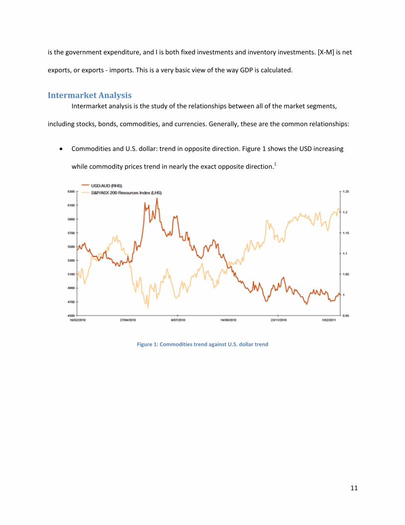
Intermarket Analysis Intermarket analysis is the study of the relationships between all of the market segments,
including stocks, bonds, commodities, and currencies. Generally, these are the common relationships:
Commodities and U.S. dollar: trend in opposite direction. Figure 1 shows the USD increasing
while commodity prices trend in nearly the exact opposite direction.1
Figure 1: Commodities trend against U.S. dollar trend

12
Commodities and bonds: trend in opposite direction as seen in Figure 2.2
Figure 2: Commodities and bond trends over 3 years.
Stock prices and bond prices: trend in same direction as seen in Figure 3.
Figure 3: Stock and bond prices over 12 years
The U.S. Dollar index and the Reuters Commodities Index trend in the opposite direction 90% of the
time.3 A lower value of the dollar is good for commodities because when the U.S. dollar is lower it
entices other countries to purchase American goods, therefore boosting exports. Higher demand for

13
American commodities means prices will go up. On the contrary, raising commodity prices can be seen
as a sign of future inflation. The Federal Reserve counters this by raising interest rates, and as a counter
effect bonds prices will drop.
Figure 4: U.S. dollar and gold over 10 years
There is a strong negative relationship between the U.S. dollar and gold prices as seen in Figure
4.4 When people see that the economy is weak or struggling, they buy precious metals, such as gold,
that won’t lose their value when the economy sinks. Oppositely, when the economy is doing well people
no longer feel the need to be safe and buy gold, so the demand drops and the prices also drop. The
dollar and oil prices are also negatively correlated.
Another interesting correlation between stocks and bonds is the fact that (almost) always the
curve for bond prices will peak before stock market. In addition, stocks hit their peak before the
commodities do. This means that bonds are an indicator of upcoming changes in the stock market, and
stocks are an indicator of upcoming changes in the commodities market.
Sectors in the Stock Market The market is made up of 10 main sectors:

14
1. Healthcare (Johnson & Johnson, Pfizer, GlaxoSmithKline)
2. Financials (Wells Fargo, JP Morgan Chase, Berkshire Hathaway)
3. Oil and Gas (Exxonmobil, Chevron, Royal Dutch Shell)
4. Utilities (Southern Co., Duke Energy, National Grid)
5. Consumer goods (Coca Cola, Proctor & Gamble, Toyota Motors)
6. Technology (Google, Apple, IBM, Microsoft)
7. Industrials (General Electric, Raytheon, 3M)
8. Telecommunications (AT&T, Verizon, Vodafone)
9. Consumer Services (Wal-Mart, Amazon, Home Depot)
10. Basic (E.I. DuPont de Nemours, Syngenta, BHP Billiton)
Figure 5: Main sectors of the stock market broken into industries.

15
All of these sectors are broken up into smaller industry groups, and then individual stocks on the
smallest level.5 Figure 5 shows a map of all of the main sectors and the individual industries current
status designated by color. Dark green designates an industry doing well and dark red designates an
industry doing poorly. A basic trading strategy is to monitor the sectors, find out which sector is the
strongest, find the strongest industry group within that sector, and then buy shares of the strongest
stocks in that group. This can also be done the other way around by shorting the weakest stocks of the
weakest sector.
Industry Groups Industry groups and futures can be tied closely. For example, industry groups that are heavily
affected by changes in interest rates (utilities, financials) will often rise when bonds prices rise.
Commodity-related stocks will do well when the commodities they are related to are going up in price.
For example, a spike in aluminum prices would highly benefit the stock of Alcoa Co, an aluminum
producer. A rise in oil prices is good for energy companies such as Shell and Chevron, but since stocks
generally lead commodities, an increase in the stocks of Shell would be an indicator of raising oil prices
in the near future.
Sector Rotation Throughout the economic cycle, big money-moving institutions, such as banks, transfer, or
“rotate,” their investments to different parts of the market. The amount of money they move can
actually change the prices of stocks, bonds, commodities, and other things, so it’s a wise decision to
follow these large companies and move your money with them.

16
Figure 6: Cyclical and defensive stocks over 2 years
Cyclical stocks and defensive stocks are always battling each other.6 Cyclical stocks are stocks
that fluctuate with the economy. When the economy is doing well, people tend to buy shares in cyclical
stocks because they are on the rise. When the economy is weak and bond prices are high, cyclical tend
to do poorly and people invest in defensive stocks, such as utilities, because they are hardly affected by
changes in the economy. Figure 6 shows that when the economy changes in direction, cyclical and
defensive stocks change roles.
The stock market always hits its trough before the economy does; i.e. the economy’s status is
largely based on how the stock market is doing. The price of oil has historically been the turning point of
the economy’s cycle; every recession since 1960 has followed a jump in oil prices. When the economy is
nearing the end of the “boom” part of its cycle, the Federal Reserve responds to inflationary pressure by
increasing interest rates. Next, oil and materials stocks will start to rise more slowly than the rest of the
economy, this is a sign that the economy has hit its peak and a downturn is imminent. When utilities and
staple-related stocks start doing better, that is a sign that people fear a recession and are investing in
things that people need, such as food and electricity, because they are low-risk. Sector rotation is a cycle
that goes hand in hand with the economy. Smart investors will exploit the cycle.

17
Stock Market Indices The three main stock market indices are the Dow Jones Industrial Average (DJIA), Standard &
Poor’s 500 (S & P 500) and the NASDAQ 100. The DJIA started in 1896 and began as an average of the
prices of the top 12 companies on the New York Stock Exchange, which at the time were all industrial
corporations due to the industrial revolution. Today, the Dow is a price-weighted index, which means
that the stocks with higher prices contribute more to the DJIA’s value. It also consists of 30 corporations
now, and they aren’t all industrial.
Since 1946, the S&P 500 has been a market value-weighted index, which means each stock in
the index is weighted based on its market value. The S&P 500 is widely known as the index that best
represents the stock market as a whole. A committee chooses the top 500 large cap stocks based on
factors such as liquidity, market size, and industry, and puts them all in one index.
In 1985, the NASDAQ 100 was created in order to capture the technology stocks that were
developing at the time. It, like the S&P 500, is also a market-weighted index, but it differs because it is
mainly comprised of technology stocks such as Microsoft, Cisco, and Facebook. Figure 7 show how all
three indices trend similarly because they are trying to represent the economy. These are the three
most commonly used indices; however there are many more indices available for use by different types
of traders.7
Figure 7: NASDAQ 100, S&P 500, and DJIA replica stocks that show the trend of the economy over 13 years.

18
Trading System Development There are trading systems, such as Tradestation, that make it easy to plot a symbol on a chart
and conduct a variety of analytics, such as implementing indicators, back testing, and optimization. Most
platforms are only used for research and testing, but some like Tradestation are also brokers and can be
used to buy and sell financial items while also conducting research, providing live news feeds, a scanner,
and a computer language used to develop trading strategies.
Any trading system must have these key components:
A clearly stated objective
A market to trade (stocks, bonds, futures, etc.)
A time period over which trades would occur (minutes, months, years)
Entry and exit rules
Position sizing and risk management rules
System Monitoring techniques
Asset allocation rules
Manual and Automated Trading Styles Manual and automated trading are similar on many levels but also take different personalities to
successfully trade. Manual trading is when a human directly offers a trade for a stock in some way.
Automated trading is when a human creates a program that will trade for them. These programs are run
through a software trading platform such as Tradestation.
Manual trading takes a personality where the human has to know exactly how the stock will
move in the future. News is one major part for the manual trader. If a trader worries or is impatient

19
when looking at a stock, it can drastically harm his net profit. One well known fact about manual traders
is that they must stick to their own rules to get good results.
Automated traders can have various types of personalities. A program that is based on one or
more mathematical algorithms will always follow the rules that are programmed into it. The idea of
automated trading is that there is some scientific motion that stocks usually move in and a program
should be able to recognize it and use it to their advantage. News still will affect someone who trades
autonomously and can actually harm a program from running as desired. A manual trader can use a
program to create indicators like an automated trader but still make the choices manually instead of
relying on a computer to successfully trade.
Basic Strategy Techniques
There are several basic strategy techniques that are necessary to know to trade successfully.
Three of the strategy techniques are trend following, volatility trading, and specialized trading. Each of
these techniques can be successful if used appropriately.
A trend following system is probably the easiest strategy technique to learn. A trend following
strategy uses the long term ups and downs to gain profit. It is called a trend following strategy because it
follows the up and down trends of the stocks. It is fairly simple and can be very affective.
A volatility strategy is a little more complex but still understandable. Volatility is practically how
much noise there is in a system. The more spikes there is up and down in a stock, the more volatility it
has. A volatility strategy uses the large ups and downs of a stock to gain profit in a smaller period of
time.
20
A specialized strategy is exactly what it sounds like, a strategy that is specific for a special
scenario. The variety of a specialized strategy is endless. Examples of specialized strategies are ones that
look for news related spikes, morning trading, night trading, or even directionless trading.
Advanced Strategy Techniques
Expectancy and Profitability
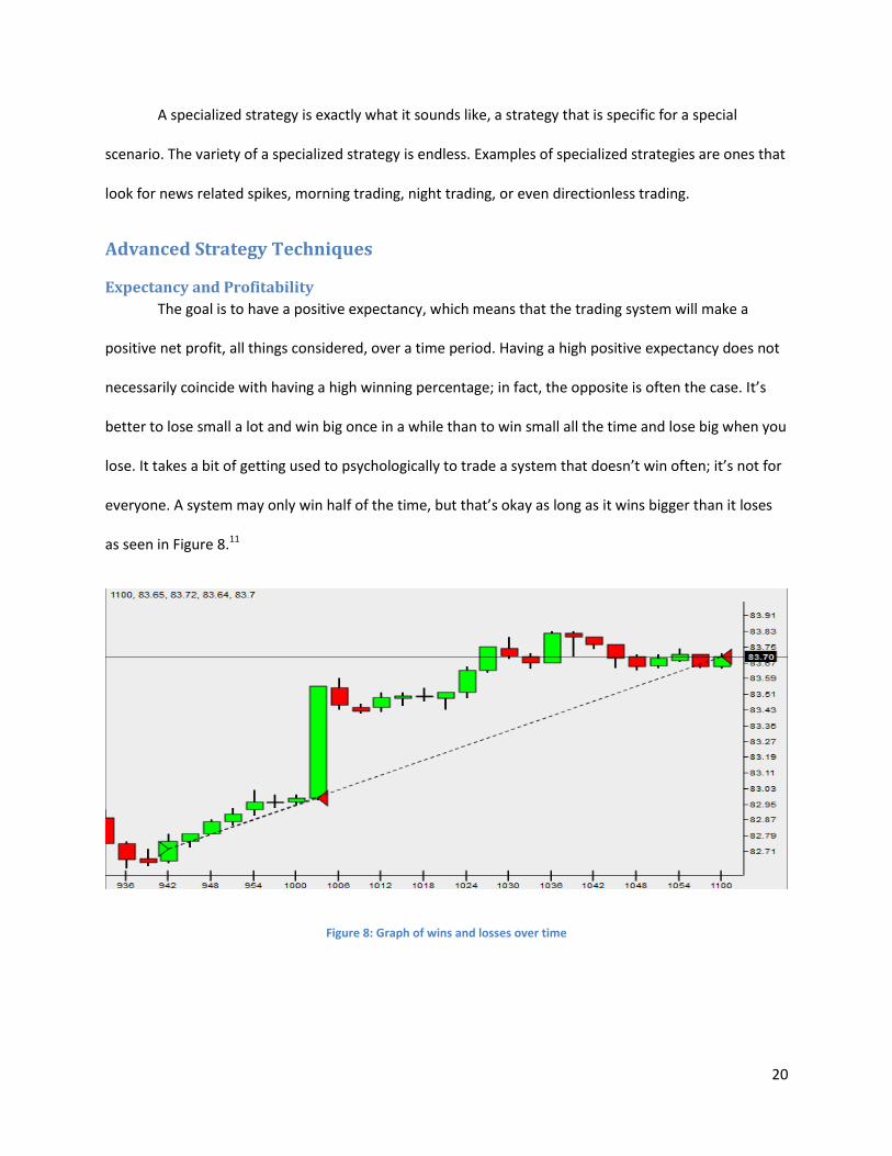
The goal is to have a positive expectancy, which means that the trading system will make a
positive net profit, all things considered, over a time period. Having a high positive expectancy does not
necessarily coincide with having a high winning percentage; in fact, the opposite is often the case. It’s
better to lose small a lot and win big once in a while than to win small all the time and lose big when you
lose. It takes a bit of getting used to psychologically to trade a system that doesn’t win often; it’s not for
everyone. A system may only win half of the time, but that’s okay as long as it wins bigger than it loses
as seen in Figure 8.11
Figure 8: Graph of wins and losses over time

21
Expectancy is the average profit (or loss) per dollar that is put at risk in a trade. E = ∑ Ri / n
where R is the risk multiple and n is the number of trades. The breakeven point is the point at which
profit begins to occur; in this case E = 0. The Profitability Rule goes as follows:
P = 1 / [ 1 + ( WAverage / LAverage )], where W/L is the average amount of winning trades over average losing
trades. It goes to show that as long as a system wins big, it doesn’t need to win frequently to be
profitable. The Profitability Factor determines if a system is profitable; it is the summation of winning
trades divided by the summation of losing trades. If the number is greater than one, then the system is
profitable. The above trading basics form a basis for which a trading system can be constructed. Some
traders can handle only winning occasionally (but they win big) and others, especially traders that are
trading for another person, must utilize a system that has a high winning percentage in order to keep
their customers from getting worried.
Position Sizing
Position sizing rules involve the size of the position taken, i.e. the amount of shares bought, in a
trade. These rules determine the potential reward for a given trade and also determine what the loss
could be in a trade. The goal is to find the optimal amount of shares to buy. If too many are bought, it is
likely that the trader’s system will hit maximum drawdown before it can begin to make gains. If too little
are bought, then commission costs could outweigh any gains that were made. Position sizing techniques
usually go together with entry and exit rules, the most popular technique being anti-Martingale
(increase position after gains, decrease after loss).
Exploiting the Majority
A quality trading system must have some sort of creativity and be different, even slightly, than
the majority of systems. One of the best ways to gain an edge on other investors is to understand
common trading practices and exploit them. Many traders will trade predictably, follow the crowd,
overreact to price drops, or have very low patience. If a smart trader can figure out when the masses are

22
going to trade, he or she can almost predict where the market is going to move, thus vastly increasing
expectancy. In addition to being creative, having a strong exit strategy and trading in a liquid market are
also imperative to having a profitable trading system.
Entry and Exit Rules
Entry rules determine how a system will get into the market and how often. Entry rules are the
first step of a trading system, but they are also can be one of the least important; this is ironic because
traders tend to spend a good amount of their time searching for the right stock to buy. Entry rules have
one job—to make sure that the system picks up all stocks that fit the trader’s criteria.
Entry rules can be divided into setup entry rules and trigger entry rules. Setup rules determine if
the market is generally favorable for the system to trade. They don’t initiate trades; they just observe
the state of the market by looking at things such a sector rotation, the news, the economic calendar,
patterns, and psychology of the masses. Trigger rules tell the system (if automated) to “pull the trigger”
and trade immediately. Trigger rules confirm the setup rules validity by picking up on a price move in the
same direction indicated by the setup rules, and then choosing a certain order type (market, limit, etc.)
to get into the market with.
Exit rules, which are extremely important and relevant to the expectancy of the system, come in
four categories, the first being Discretionary. These rules are made to prevent the system for failing due
to inability to operate as desired. For example, if the computer used to trade freezes or crashes, these
rules will be able to detect the problem and take action to prevent loss. It also notices when the
market’s liquidity has dropped and when firms that the trader invests in are being sold or are merged.
Inactivity Rules are made to sell positions that have been stagnant and held for a long time, therefore
generating risk without generating profit. The length of time that is considered “too long” is based on
the average trade duration of the system and the amount of price change that deems a financial

23
instrument stagnant is based on the volatility of the instrument that is being traded. There are also
Profit Exit Rules, which have the goal of exiting a position at the point at which it is unlikely any more
profit will be gained from the position. These rules can be designed to sell shares in a staggered manner
so that the trader can slowly exit a position. Finally, it’s important to have Loss Exit Rules, which prevent
losses from becoming too large. The goal of these exit rules is to determine, based on volatility and
price, if a position has failed at accomplishing the trader’s goals and consequently sell.
Trading Indicators
Support and Resistance
Support and resistance are one of the underlying concepts that must be understood by a trader.
Support is simply the price at which demand stops the price from declining any lower; this is known as
the “floor.” Resistance is a resistance to an increase in price due to selling; this is often called the
“ceiling.” Identifying floors and ceilings is crucial to trading successfully. Traders use tools like trend
lines, regression channels, and Fibonacci sequences and also look at recent and historical highs/lows to
determine if a price is at a floor or ceiling. The most important thing to identify is a breakthrough, which
is when a stock breaks through a resistance or falls through a support. When a stock breaks through the
ceiling, the ceiling often becomes a new floor. On the contrary, a floor often becomes a new ceiling
when a stock drops through.8 An example ceiling and floor of a stock can be seen in Figure 9.

24
Figure 9: Support and resistance of a stock
Trend Lines
Trend lines, which are made of two or more price points, continue as a straight line into the
future and are used as a support or resistance line. Up trends (which are drawn from lowest-low to
highest-low) and down trends (highest-high to lowest-high) can be easily made using computer
software, which also can help with determining breakthroughs. Trend lines can either be semi-log or
arithmetic; semi-log often gets a straight line and arithmetic produces multiple straight lines, which
change in steepness. Steepness is very important because it is a sign of how quickly something is
trending. If a stock price is going upwards at a slight, consistent pace and then suddenly the slope
increases greatly, the stock may have broken through the resistance.
Moving Averages
Moving averages are another way of determining points of support and resistance. The most
common forms are the simple moving average and exponential moving average. Both moving averages

25
are used as trend following indicators. These indicators normally are used as an indicator for the
direction of trend that the stock is currently moving in.
The simple moving average is the most basic mathematically. The simple moving average is
calculated by summing up the close of the stock over a period of time and dividing by the number of
stock closes over that period of time. It is mathematically the same as taking an averaging of any set of
data.
The exponential moving average uses weights to create a moving average that is closer to being
the actual stock. The exponential moving average (EMA) calculation can be seen below:
EMA = {Close - EMA(previous day)} x multiplier(weight) + EMA(previous day)
The multiplier (weight) allows it so that more recent data is taken to be more important than past data.
In Figure 10, the differences between simple and exponential moving average can be seen visually.9
Figure 10: Simple and Exponential Moving Average

26
Bollinger Bands
Bollinger bands are an indicator that also works as support and resistance. Bollinger bands
normally consist of two bands that anticipate the highest high and lowest low of the stock. If a
breakthrough occurs through one of the bands, it is likely that it will continue in that direction for a
short period of time. Bollinger bands are simply calculated as the simple moving average plus or minus
the standard deviation of the simple moving average. The Bollinger band technique can be fairly
effective in spotting breakthroughs as seen in Figure 11.13
Figure 11: Bollinger Bands with breakouts
Average True Range
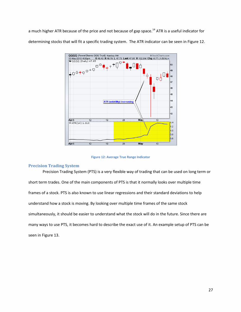
The average true range (ATR) is an indicator that measures volatility. This indicator does not
show direction of the stock but how large of a range the stock normally is within. The true range is
calculated by simply seeing the largest difference between the previous close and the current high or
low. ATR is normally used on a daily, weekly, or monthly basis to determine how a stock normally
moves. The ATR value is dependent on the stock that it is being applied to. A higher cost stock will have
27
a much higher ATR because of the price and not because of gap space.14 ATR is a useful indicator for
determining stocks that will fit a specific trading system. The ATR indicator can be seen in Figure 12.
Figure 12: Average True Range Indicator
Precision Trading System
Precision Trading System (PTS) is a very flexible way of trading that can be used on long term or
short term trades. One of the main components of PTS is that it normally looks over multiple time
frames of a stock. PTS is also known to use linear regressions and their standard deviations to help
understand how a stock is moving. By looking over multiple time frames of the same stock
simultaneously, it should be easier to understand what the stock will do in the future. Since there are
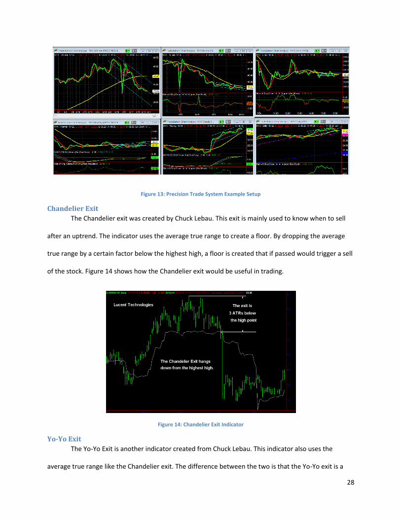
many ways to use PTS, it becomes hard to describe the exact use of it. An example setup of PTS can be
seen in Figure 13.
28
Figure 13: Precision Trade System Example Setup
Chandelier Exit
The Chandelier exit was created by Chuck Lebau. This exit is mainly used to know when to sell
after an uptrend. The indicator uses the average true range to create a floor. By dropping the average
true range by a certain factor below the highest high, a floor is created that if passed would trigger a sell
of the stock. Figure 14 shows how the Chandelier exit would be useful in trading.
Figure 14: Chandelier Exit Indicator
Yo-Yo Exit
The Yo-Yo Exit is another indicator created from Chuck Lebau. This indicator also uses the
average true range like the Chandelier exit. The difference between the two is that the Yo-Yo exit is a

29
factor below the current close rather than the highest high. Similarly, when this line is passed, a sell is
trigger to show that an uptrend is finished. This exit is not normally used alone and is used to find
volatility abnormalities in the opposing direction. Figure 15 shows how a Yo-Yo exit would create a sell
trigger before the stock drops too much.
Figure 15: Yo-Yo Exit Example
Modified Parabolic Exit
The Modified Parabolic exit is the final of the three exits created by Chuck Lebau. This exit uses a
trailing stop that moves closer and closer to the current price as new highs are made. There is an
acceleration factor that is used with the Modified Parabolic exit that sets how fast the floor will move up
when new highs are met. Figure 16 shows how a Modified Parabolic exit works by showing the floor as
white dots.

30
Figure 16: Modified Parabolic Exit Indicator
Stock Screening The best way to find stocks that meet the criteria of a trading system is to utilize stock
screeners. The two basic types are fundamental stock screeners and technical screeners, both of which
can be either online or downloadable to a computer for quick and easy (but not always free!) access.
Fundamental stock screeners use numerical data (i.e. quantitative data) to filter the massive
amount of stocks into small piles that meet criteria chosen by the trader. This is a quick way to stumble
upon stocks that might have been otherwise overlooked had they not been found by the screener. Also,
traders may question their criteria after seeing the scanner grab stocks that they would rather not trade.
A common problem with fundamental scanning is that the user applies too many criteria and the
scanner only returns a very small amount of stocks. Other stocks that, for example, meet 5 out of 6 of
the criteria won’t show up in the scanner, which could result in the trader missing out on some near-
ideal stocks. Stubborn stock screening will not yield good results; being flexible and adjusting
parameters is very important. After scanning possibly multiple times, it’s imperative to research the
stocks that appear in the screen, especially the ones that you know very little about. A stock may appear

31
in a screen that looks perfect, but upon further research the trader may find that this particular stock is
predicted to take a turn for the worse in the future. Fundamental screening can be very effective as long
as there are defined objectives and criteria and research is done after scanning for stocks. Figure 17
shows an example of a scan from Google Finance. 10
Figure 17: Scan from Google Finance
When screening, it’s very important to do a secondary scan in addition to the primary scan to
avoid getting certain stocks just by coincidence. The goal of primary screening is to find the stocks that
meet the trader’s objectives by offering a comparison between a firm’s numbers and the numbers of
something else, such as the market as a whole or possibly another firm. A common problem with
primary screening is that the trader set up the screener in such a way that it as counter-productive
objectives. For example, scanning for dividend stocks and stocks that are showing signs of growth would
potentially cancel each other out.

32
Secondary screening is a more “fine” filter that makes sure the stocks that made it through the
primary screen did not get there because they coincidentally fit through the screen, but because they
truly meet the trader’s objectives. For example, a primary screen may find stocks that have risen more
than 5% over the past week. The secondary screen may come through and weed out all of the stocks
that have a very low price because the cost of commission would outweigh the gains of the smaller-
priced stock. There are many sites and also some trading platforms that can do these types of scans.
Back-Testing and Optimization Back-testing and optimization are methods used to produce and perfect a trading system. They
can use exhaustive techniques that take time to review past data or they can use probabilistic
techniques that use prediction and past data. When back-testing it is important to avoid looking at the
noise of a chart and look closely at the actually movement. It’s also extremely important to realize that a
system that worked well in back-testing will not necessarily work well in the future. Walk-forward
analysis can be done to see how a trading system may perform in the future.

33
Methodology
Jason Howell’s Trading Strategy
My trading system is a long term and trend-following, the basis of it is a crossing two
line exponential moving average system. This means that the exponential moving average
(EMA) of a particular symbol, on a particular time frame, for certain number of bars back, is
compared to the EMA for the same symbol, on the same time frame, but for a different number
of bars back. The system trades Google stock on 80 minute bars. I used 80 minute bars
because they produced the most net profit in back testing when compared against many
different bar lengths. Several of the bar lengths that were tested were 30, 35, 60, 66, 70, 80
and 90 minutes. There are two important things to take way from the results of these tests.
One, as previously stated the 80 minute bar length worked best and two; the 30, 60 and 90
minute bar lengths work the poorest. This could be because the 30, 60 and 90 bar lengths are
more commonly used. The general idea of a simple two line EMA system is that when the EMA
that looks at the shorter number of bars back, (the short EMA), is greater than the EMA that
looks at more bars back, (the long EMA) the market is bullish. Conversely, if the reverse is true
then the market is bearish. So, in general, when the short EMA crosses over the long EMA that
particular symbol is likely to increase, and one should consider entering a long position or
exiting a short position. Furthermore, when the short EMA crosses under long EMA that
particular symbol is likely to decrease, and one should consider entering a short position or
exiting a long position. This alone, however, does not make for a good system; there are a few
problems with just using a simple two line EMA system.

34
Problems with Two Line EMA System and Attempted Solutions
One major problem with simply using a two line EMA crossing system is that it does not
give you all the information about if a symbol will move up or down. If the short EMA crosses
over the long EMA, that is merely one indication that the symbol might move up in the near
future. It is best to tweak this type of system or to use it with another indicator. Since the
system I made only takes long positions the most basic entry rules I could use would be to buy
long x number of shares after the short EMA crosses over the long EMA. The most basic exit
strategy would be to sell x number of shares after the short EMA crosses under the long EMA.
Instead of doing that I decided to tweak the entry rules to make them more selective and to use
a more sophisticated exit strategy. I will get into the details of my strategy and how I got there
in a later section. For now I will go through more problems with
Entry Rules
The first idea I had to tweak the two line EMA crossing system was designed to avoid
getting in and out of the market too frequently. With a simple two line EMA crossing system it
is possible for the short EMA to cross over the long EMA and then cross back under on the next
bar. If you have a long only system like I do, and this is all you had for entry and exit strategies
then you would buy long and then sell on the very next bar. This causes a few problems. One, if
that trade was a winning trade, it probably wasn’t very profitable just because it was only held
for one bar which means commission will have a greater impact on it, and might turn some
seemingly winning trades into losing trades. Of course this problem can basically be ignored if
you use a large enough position size, because a $16.00 commission probably won’t be enough
to make a winning trade become a losing trade if you are trading several hundred shares of
Google for example. Another problem is that when an entry or exit rule is met, the system will

35
buy/sell “at next bar”. So, in this case it would buy long on the bar that the short EMA crossed
under the long EMA and sell on the next bar. This is the opposite of what you would want to do,
you would have bought long right when the system was indicating the symbol would move
down because the bar before it indicated the symbol would move up. So it could be possible
that the short EMA went over the long EMA by only a penny and then went below the next bar
by only a penny. If that happens then the symbol is basically just moving sideways and you
would be just trading the noise and probably losing money overall. So, it is logical to try to
avoid this problem.
The general solution to this problem that I used was to wait for the short EMA cross
over and get far enough above the long EMA. This tries to make sure the symbol has enough
momentum in the direction you want before you take a position. So now the obvious question
is how far is far enough. I tried a few ways to solve this problem. The first way I tried looked at
the quotient between the value of the short EMA and the value of the long EMA. This quotient
had to be greater than a certain value in order for a position to be taken. That value was
optimized in TradeStation. It should be noted that this value should be slightly greater than
one. If it is one that means that the value for the short EMA and long EMA are exactly equal;
that is to say it is a crossing point. Let’s assume that TradeStation optimizes this value to 1.05,
this means the price of the short EMA has to be at least 1.05 times greater than the long EMA
before a position is taken. A second method I tried was dividing the short EMA by the sum of
the short EMA and long EMA and wait for that quotient to get above a certain optimizeable
threshold before taking a position. In this case a crossing point where both EMAs are equal
occurs when this quotient is 0.5. The system would only take a position if this quotient went

36
above the threshold, which might be something like 0.505. The last method I tried, and the one
I finally used in my strategy, was simply looking at the difference between the short EMA and
the long EMA. Like the others, this system would not take a position until the difference
between the short EMA and the long EMA was great enough. Again this number can be
optimized. If TradeStation optimizes this number to 1.0 for example, that means the system
will not take a position unless the short EMA gets at least $1.00 above the long EMA. I decided
to use this method for my system’s entry strategy simply because out of the three, it worked
the best in back testing. By that I mean, the entry using the difference between the EMA’s
optimized to the most net profit. The optimizations were done in mid-February of 2013 on
Google using 35 minute bars and 100 days back. The exit was kept the same for these
optimizations.
Exit Rules
After finding that these tweaks worked well for the entry I tried the same three
methods for the exit. For the exit strategy it made the most sense to wait to sell until the two
EMAs got close enough together again. Let’s consider the difference method for an example. If
TradeStation optimized the difference to 1.0 then the difference between the short EMA and
the long EMA would have to fall below $1.00 before the position was sold. I tried all exits with
their respective entries and the difference method still worked the best. After looking at many
different graphs showing historical testing of that system it was clear that it left the market too
late. By that I mean the price of the stock peaked, went down some and then was sold. This
didn’t occur every trade of course, but it was a definite pattern. Another thing I noticed was
that the price peaked close to when the short EMA started decreasing. From this observation I

37
decided to change the exit strategy to one that sold the position after the short EMA decreased
for two consecutive bars and also decreased by a great enough amount. These two
parameters are designed to insure that the price of the stock has actually peaked and that it is
unlikely to go higher. I decided to wait for the short EMA to decrease for two consecutive bars
instead of just one because one bar wasn’t enough evidence for me that the stock price
wouldn’t continue to go up. I wanted to avoid instances where the short EMA would decrease
by a few cents for two bars in a row, knocking me out of the market, only for the price of the
stock to increase right after. The way I decided to avoid this scenario was by creating a
threshold amount that the short EMA would have to decrease by before the position was sold.
This amount is an input that you can optimize in TradeStation. A little while later I decided to
change my exit strategy again. First I tried to incorporate Charles LeBeau’s three stops into my
system. His three stops are the “Chandelier” exit, the “Yo-Yo” exit, and the “Modified
Parabolic” exit. The “Chandelier” stop is set at a point some distance (about three average true
ranges) below the highest high since the trade was made. The “Yo-Yo” stop is a stop set some
distance (usually about 2 average true ranges) below the most recent close. The “modified
parabolic” stop is a stop that gets closer to the price of the stock the longer the position is held.
I originally tried using these three exit strategies in combination with the last one described
above. However, it became evident through back testing that using just Charles LeBeau’s exit
strategies worked the best and it is the exit strategy my final system uses.
Position Sizing
The last part of the code I did was for position size. Many traders agree that an Anti-
Martingale strategy works best for position size. An Anti-Martingale strategy is one where your

38
position size increases after a winning trade and decreases after a losing trade. The way I
implemented this was by initially risking a certain percentage of the capital I had for the
simulation ($100,000). I then increased or decreased the amount I risked for each trade
depending on the previous trade. If the previous trade was a winning trade, the amount risked
would be increased by a certain percentage for the next trade. If the previous trade was a
losing trade then amount risked would be decreased for next trade. These percentages don’t
need to be equivalent but they should be relatively close or else a long string of either losing or
winning trades could distort your equity curve because of this unlikely event. You should
determine the initial percentage of your starting capitol that you are willing to risk before your
first trade. For my system, the percent of initial capitol risked on the first trade is 40%. This
number can vary greatly and should be what you are personally comfortable with. You should
also determine the percent increase after a winning trade and the percent decrease after a
losing trade. For my system, I increased the position size by 5% after each winning trade and
decreased it by 4% for each losing trade.
Ben McIntyre’s PTS Strategies Several PTS strategies were implemented to determine which of the strategies was the most
profitable. There are three different attempts at using a linear regression and PTS to create a successful
system. The first attempt was named PTSrocket for the use of a volatility detecting strategy introduced
inside of a PTS article. The second attempt was named PTStrending because it used a trending technique
with ceilings and floors. The last attempt was named PTSmulti because it used trending tactics with
multiple time frames to find the dynamics of the stock.

39
PTSmulti Objectives
The overall goal of the PTS multiple time frame (PTSmulti) strategy is to help understand the
dynamics of a stock and use them to create trade with profit. The PTSmulti strategy is an imitation of a
manually traded PTS strategy in [1]. High winning percentage is fairly important but only small losses
should be made by the PTSmulti strategy. There is an aim to have a low max drawdown. The PTSmulti
strategy should be robust across most markets and most time frames. This strategy should only spend
time in the market where larger differences in price occur and very little to no time spent in a
directionless environment. This strategy also does not trade overnight or within a certain time period of
the morning. This is due to the fact that a lot of volatility or unexpected change in stock value occurs at
this time. Depending on the time period that the user chooses, the time commitment can be very small.
The strategy must be very simplistic and easy to optimize so that too much time isn’t spent out of the
market.
Particular stocks for PTSmulti
Choosing the correct stocks for a strategy can greatly improve performance. The PTSmulti
strategy was created for trending stocks. A higher daily average true range is preferred due to the fact
that this means that the stock is always moving in a downtrend or uptrend. The more noise and volatility
at the close, the harder it is for the strategy to find the optimal values. A smaller time period naturally
has more volatility so finding the dynamics of these stocks is much more difficult. For this reason, the
strategies performance for a smaller time period is less effective than a larger time period. A high
liquidity for the stock is very important because without liquidity, it is much harder to make trades occur
when the strategy wants them to. This strategy was mainly tested on Google from time periods of 20 to
80 minutes.
Entries and Exits for PTSmulti
The PTSmulti strategy was an autonomous strategy that used two linear regressions in different
time frames and their slopes to determine when to buy and sell. When an optimized slope value was

40
passed above, the strategy would buy. When this optimized slope value was passed below, the strategy
would sell. This was implemented as only one linear regression in one time frame and then with two
linear regression in two time frames. When two time frames were used, both optimized slope values
had to be passed to buy and it would sell when only the smaller time frame linear regression’s slope was
below an optimized value. This strategy had to be implemented in a single chart rather than using
separate time frame charts like seen in a tradition PTS strategy. Figure 18 shows how the strategy would
be implemented with one time frame. Figure 19 shows how the strategy was implemented with two
time frames.
Figure 18: PTSmulti with only one linear regression
As seen in Figure 18, when the slope, red line, crosses over the optimized slope value, blue line,
it signals a trade to occur. It practically is buying when the graph starts going upwards and sells when
the graph starts going downward. This simple strategy can work in any trending environments that are
mostly going upward. A simple way to filter out the bad trades is by adding a longer time period linear
regression that looks at the overall trend of the stock.

41
Figure 19: EasyLanguage for PTSmulti with one linear regression
Figure 20: PTSmulti with two linear regressions
Figure 20 shows the PTSmulti strategy with two linear regressions. The trades will now only
occur when both of the slopes of the linear regressions are greater than their corresponding optimized
slope factors. The blue and red lines remain the same as for the one linear regression. The cyan line is
the optimized factor for the longer linear regression slope, and the yellow line is the slope of the larger
linear regression. By comparing Figure 18 and Figure 20, it can be seen that no trades have been
changed. The reason why the larger linear regression is placed in is to take out the bad trades as seen in
Figure 22.

42
Figure 21: EasyLanguage for PTSmulti with two linear regressions
Figure 22: PTSmulti with two linear regression filtering
In Figure 22, there are no trades being made because the longer linear regression is now under
the optimized slope factor. Without the longer linear regression, trades would occur that would cause
loss because of the overall downtrend of the stock.
PTSrocket Objectives
The overall goal of the PTSrocket strategy is to use the large, quick changes in stock price to gain
profit. The PTSrocket strategy is an imitation of a manually traded PTS strategy. High winning percentage

43
is very important because this strategy is not traded very often along the same stock. The PTSrocket
strategy should be robust across most markets and only the smallest time frames. This strategy should
only spend time in the market where larger differences in price occur and no time spent in a
directionless environment or trending environment. The time commitment for this strategy is very
small. The strategy must be very simplistic and easy to optimize so that too much time isn’t spent out of
the market.
Particular stocks for PTSrocket
The PTSrocket strategy was created to trade on stocks that have a high volatility over a short
period of time. The stocks that are best to trade are ones that have news about them coming out soon.
This is due to the fact that large changes in stocks usually occur when news is revealed. The less volatility
that the stock normally has without news being revealed is better for this strategy. Having less volatility
normally allows the detection of large change to be much easier. A smaller time period is needed so that
the PTSrocket strategy can react faster. Using a larger time period stock would never be very effective
for trading based on news. A high liquidity for the stock is very important because without liquidity, it is
much harder to make trades occur when the strategy wants them to. This strategy was tested on the 1
minute time frame on multiple stocks that had large spikes of change because of news.
Entries and Exits for PTSrocket
The PTSrocket strategy was an autonomous strategy that mimicked a news relative manually
traded strategy. The idea of the system was fairly simple in that it created a ceiling and floor and used
the volume of the stock as an indicator. If the volume of the stock was higher than normal and the close
of the stock passed a ceiling or floor, a trade would be made to go along with the breakthrough or
breakdown. The ceiling and floor were optimized factors plus the current linear regression value. In the
manually traded strategy, the ratio between the average volume and current volume were used as an
indicator for telling if the stock seemed like it was going to breakthrough a ceiling or floor. The ratio of

44
current volume to average volume was also an indicator as the fuel of the rocket. If the ratio was large,
the rocket would continue going in the same direction. If the ratio was approaching 1, then there would
no longer be a rocket. The slope of the linear regression was also tested as a trigger of when to sell or
buy. For example, after buying during an uptrend breakthrough, if the slope of the linear regression
starts to turn downward by a certain factor, it would sell due to the fact that the stock is moving away
from the previous uptrend. A buy stop was later introduced into the breakthroughs to see if it would
take fewer losses. The parameters being optimized for the simplest version were the length of the linear
regression, the length for the average of the volume ratio, the factor added to the linear regression
value for the ceiling, the volume ratio that must be passed to make a trade, the volume ratio that must
be passed to end a trade, and the slope that would determine to sell after an uptrend. A basic code
example is shown in Figure 23.
Figure 23: PTSrocket simple variation of code
The variables BuyRat, SellRat, buyNum, and SellSlope are directly optimized numbers while
slope, LRV, and VolRatioAvg are affected by optimizing the length of the linear regression and length for
the average of the volume ratio. LRV is the current linear regression value. The variable tempBought is

45
just used for guaranteeing that 100 contracts are used for every trade. Figure 24 shows an example for
the desired trades that PTSrocket will make.
Figure 24: The best scenario and intent for PTSrocket
PTStrending Objectives
The overall goal of the PTStrending strategy is to use the up and down trends of stocks to gain
profit. High winning percentage isn’t very important as long as it only loses small amounts of money.
The PTStrending strategy should be robust across most markets and larger time frames. This strategy
should only spend time in the market where uptrend and downtrend occur and little to no time spent in
a directionless environment. The time commitment for this strategy can be all day long depending on
the stock and time frame chosen. The strategy must be very simplistic and easy to optimize so that too
much time isn’t spent out of the market.
Particular stocks for PTStrending
The PTStrending strategy was created to trade on stocks that have low volatility and very little
time being directionless. A higher daily average true range is preferred due to the fact that this means
that the stock is always moving in a downtrend or uptrend. The more noise and volatility at the close,
the harder it is for the strategy to find the optimal values. Smaller time periods have more volatility at
the close so larger time periods are more likely to get profit. A high liquidity for the stock is needed to
create trades. This strategy was mainly tested on Google from time periods of 20 to 80 minutes.

46
Entries and Exits for PTStrending
The PTStrending strategy was an autonomous strategy that used a linear regression and
standard deviations to buy and sell with the trend of the stock. The standard deviations of the linear
regression were used as ceilings and floors. There are many different ways to play ceilings and floors but
this strategy mainly looked at buying and selling related to the ceiling. The strategy would buy when the
slope was greater than some value or when the close broke through the ceiling. The strategy would sell
when the slope was less than some value or when the close broke through the floor. Buy stops were
also tested on this strategy to guarantee that a breakthrough was occurring. An offset was used on the
linear regression to make sure that the last close of the stock wasn’t used to detect breakthrough or
breakdowns. The simplest PTStrending code can be seen in Figure 25, and an example seen in Figure 26.
Figure 25: Simplest PTStrending code

47
Figure 26: PTStrending example
System Part 3: by Vinnie McMahon This portion of the overall system analyzes an article written by Mike Bryant in the Breakout
Bulletin from 2007, which has a focus on basic exit strategies. The article provides a very interesting bit
of EasyLanguage that allows traders to utilize different exit strategies using an “on/off” switch in the
code, which also contains one very basic entry rule:
Inputs: ChanLen (20), NBEnt (20), FrATR (1.0), MALen (20); Var: ATR (0), MarkPos (0), TrailOn (FALSE); ATR = Average(TrueRange, 20); MarkPos = MarketPosition; Buy next bar at Highest(H, ChanLen) + 1 point stop; Sell short next bar at Lowest(L, ChanLen) - 1 point stop; If MarkPos <> 0 and MarkPos <> MarkPos[1] then TrailOn = FALSE; { Trade entered this bar so reset trail flag } {Exit at N bars since entry} {If MarketPosition = 1 and BarsSinceEntry = NBEnt then Sell next bar at market; If MarketPosition = -1 and BarsSinceEntry = NBEnt then

48
Buy to cover next bar at market;} {Exit using a money management stop} {If MarketPosition = 1 then Sell next bar at EntryPrice - FrATR * ATR stop; If MarketPosition = -1 then Buy to cover next bar at EntryPrice + FrATR * ATR stop;} { Exit with a trailing stop } {If MarketPosition = 1 and TrailOn = FALSE and (Close - EntryPrice) > FrATR * ATR then TrailOn = TRUE; If MarketPosition = 1 and TrailOn then Sell next bar at (EntryPrice + 0.5 * (C - EntryPrice)) stop; If MarketPosition = -1 and TrailOn = FALSE and (EntryPrice - Close) > FrATR * ATR then TrailOn = TRUE; If MarketPosition = -1 and TrailOn then Buy to cover next bar at (EntryPrice - 0.5 * (EntryPrice - C)) stop;} { Exit at a profit target } {If MarketPosition = 1 then Sell next bar at EntryPrice + FrATR * ATR limit; If MarketPosition = -1 then Buy to cover next bar at EntryPrice - FrATR * ATR limit;} { Exit on a moving average crossover } {If MarketPosition = 1 and C < Average(C, MALen) then Sell next bar at market; If MarketPosition = -1 and C > Average(C, MALen) then Buy to cover next bar at market; } { Exit on RSI movement } {If MarketPosition = 1 and RSI(C, 14) crosses above 70 then Sell next bar at market; If MarketPosition = -1 and RSI(C, 14) crosses below 30 then Buy to cover next bar at market; }
The segments in green, separated by spaces, are the various exit strategies employed by Bryant.
To activate a strategy, simply remove the brackets surrounding the “If” statements and click the “Verify”
check mark in the Tradestation Development Environment. Then in the chart area, right-click and press
“Format Strategies” and add the strategy to the chart.
In order to understand the code, one must first be familiar with the exit rules that it utilizes.
Novice traders often focus much more on the entry into the market instead of the exit, which is a
49
terrible idea even though it seems to make sense. Traders focus so much on things such as moving
averages and breakout but do not know when the right time to sell/buy to cover is. Bryant says that exit
rules are “the principal method of controlling the intrinsic risk/reward characteristics of a trading
system, whether the system looks for a quick profit or holds the trade through the market's ups and
downs depends on the exits.” Exit rules can be the difference between cutting a loss short or letting the
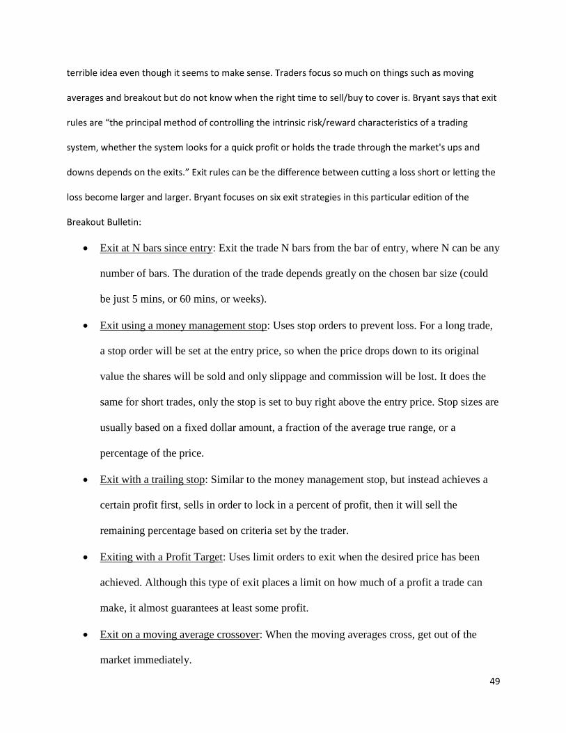
loss become larger and larger. Bryant focuses on six exit strategies in this particular edition of the
Breakout Bulletin:
Exit at N bars since entry: Exit the trade N bars from the bar of entry, where N can be any
number of bars. The duration of the trade depends greatly on the chosen bar size (could
be just 5 mins, or 60 mins, or weeks).
Exit using a money management stop: Uses stop orders to prevent loss. For a long trade,
a stop order will be set at the entry price, so when the price drops down to its original
value the shares will be sold and only slippage and commission will be lost. It does the
same for short trades, only the stop is set to buy right above the entry price. Stop sizes are
usually based on a fixed dollar amount, a fraction of the average true range, or a
percentage of the price.
Exit with a trailing stop: Similar to the money management stop, but instead achieves a
certain profit first, sells in order to lock in a percent of profit, then it will sell the
remaining percentage based on criteria set by the trader.
Exiting with a Profit Target: Uses limit orders to exit when the desired price has been
achieved. Although this type of exit places a limit on how much of a profit a trade can
make, it almost guarantees at least some profit.
Exit on a moving average crossover: When the moving averages cross, get out of the
market immediately.

50
Exit on RSI Movement: uses the Relative Strength Index to determine if it is time to get
out of the market. The equation compares the average loss to the average gain: RSI = 100
– 100/(1+RS) where RS is avg Gain/avg Loss.
In the Breakout Bulletin, Bryant came up with this system with the goal of trading futures
markets. He conducted a series of tests using crude oil (CL), E-mini Russell 2000 (ER2), Japanese Yen (JY),
T-bonds (US), and wheat (W) and then placed the data in an Excel spreadsheet for comparison as seen in
Figures 26 and 27.
Figure 27: Excel Spreadsheet of Bryant's Tests Part 1
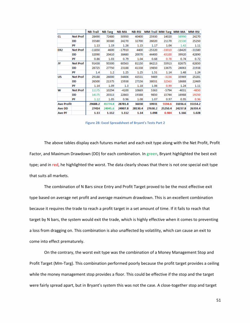
51
Figure 28: Excel Spreadsheet of Bryant's Tests Part 2
The above tables display each futures market and each exit type along with the Net Profit, Profit
Factor, and Maximum Drawdown (DD) for each combination. In green, Bryant highlighted the best exit
type; and in red, he highlighted the worst. The data clearly shows that there is not one special exit type
that suits all markets.
The combination of N Bars since Entry and Profit Target proved to be the most effective exit
type based on average net profit and average maximum drawdown. This is an excellent combination
because it requires the trade to reach a profit target in a set amount of time. If it fails to reach that
target by N bars, the system would exit the trade, which is highly effective when it comes to preventing
a loss from dragging on. This combination is also unaffected by volatility, which can cause an exit to
come into effect prematurely.
On the contrary, the worst exit type was the combination of a Money Management Stop and
Profit Target (Mm-Targ). This combination performed poorly because the profit target provides a ceiling
while the money management stop provides a floor. This could be effective if the stop and the target
were fairly spread apart, but in Bryant’s system this was not the case. A close-together stop and target

52
makes for a very small trading window, which means many small trades are made instead of less large
ones. This is bad because it induces heavy commission costs and does not allow profits to run.
The most consistent overall exit was the Target Exit and the worst overall was the RSI due to the
low profit, high drawdown, and low profit factor. The trailing stop method’s results appear to be all over
the place, probably because the trailing stop’s lock-in percentage depends on the market. The Breakout
Bulletin provides an excellent example of why exits are so important when it comes to trading
successfully. Different markets respond differently to certain exit types which means that careful
choosing of exits and optimization is required to find the exit type best suited to a particular system.
Bryant tested multiple exit types on some symbols from the futures market, but many people don’t like
to trade futures. My goal is to find out which exit is suited for the stock market.
Exit Types: Which is best suited for stocks?
My objective was to test out Bryant’s EasyLanguage code on Tradestation, but use it to find the
best exit type for Google stock on the daily bar. The reason I chose Google on the daily bar is because I
am familiar with Google and because I wanted to make a system that would suit the average person
who works 8:00-5:00 every day and doesn’t have time to keep constantly looking at the stock market.
Trading on the daily bars usually means less trades than trading on, say, 30 minute bars, which allows
traders to go about their day and not constantly have to worry about what the stocks are doing.
I used a particular set of steps to test each of the exit types for GOOG – daily. First, I entered the
Tradestation Development Environment and uploaded the code from the Breakout Bulletin. Next, I
removed the brackets around one individual exit type in the code and verified it to make sure there
were no errors in the EasyLanguage. Next, I inserted the strategy into the Google-daily chart and
optimized the four inputs (which are at the beginning of the code) using two years of historical data.
Finally, I analyzed the optimization and performance results and based their level of success on four

53
important factors: net profit, profit factor, maximum drawdown (as a percentage of initial capital), and
the number of trades made over the two-year span.

54
Results
Results of Jason Howell’s Strategy
The next two screenshots are the optimized inputs for the LeBeau exit strategy and my
EMA entry strategy respectively. These values were obtained after an optimization at the end
of April looking 100 days back and were left unchanged till the end of May while more trades
were made. The optimizations can be seen in Figures 29 and 30.
Figure 29: Lebau Exits Optimization
Figure 30: Jayson's EMA Optimization

55
Figures 31-33 show the equity curve and performance summary of the 25 trades made
from the 19th of February 2013 to the 25th of May 2013. Trades 22-25 were made after the
optimization. Some important things to notice, the system made 25 trades, in 100 days with a
56% winning percentage and a 2.94 profit factor. Those stats are pretty good, one piece of data
that can cause some concern is the return on initial capital vs. the buy & hold return. Ideally you
would want the return on initial capital to be higher than the buy & hold return; in this case
however, it was not, 5.41% vs. 8.87%. That being said however, a 5.41% return on initial capital
in 100 days isn’t so bad.
Figure 31: Equity Curve of Jason's Strategy

56
Figure 32: Performance Report of Jayson's Strategy Part 1

57
Figure 33: Performance Report of Jayson's Strategy Part 2
Results of Vinnie McMahon’s Strategy As expected, some of the exits performed well and others performed poorly. I was originally
going to modify Bryant’s simple entry strategy, but it was so effective at getting into the market and
making the perfect amount of trades (for a person who works full time) that I felt it did not need
modification. Also, it kept the trader in the market over 95% of the time, which helped gather the
highest possible amount of data regarding the exit types.

58
The best overall performer was the “N Bars since Entry” exit type, primarily due to it yielding the
highest net profit of the group. Its maximum drawdown was relatively low at 8.82% of the initial capital
of $100,000. It had a solid profit factor of 2.40 and only 27 trades were made over the two year span of
back-testing. The “Trailing Stop” and “Money Management Stop” exits were also quite effective with
their high profit factors and the lowest drawdown of the bunch, but the net profits of these exits types
were not as high as the N Bars exit. The charts and results can be seen below in Figures 34-39 and the
below table.
Figure 34: Exit at N bars since entry
Figure 35: Exit using a money management stop

59
Figure 36: Exit with a trailing stop
Figure 37: Exit at a profit target
Figure 38: Exit on a moving average crossover

60
Figure 39: Exit on RSI movement
GOOG-daily bar Trailing
Stop
N Bars since Entry
MM Stop Prof.
Target MA
Crossover RSI
Net Profit $33,093 $38,159 $29,735 $31,509 $23,203 $24,447
Max Drawdown (% of initial capital)
8.06% 8.82% 8.06% 9.93% 10.91% 10.88%
Profit Factor 2.56 2.4 2.4 1.7 1.87 1.61
Number of Trades 24 27 22 41 29 43
ChanLen 10 10 10 10 10 10
NBEnt 10 22 10 8 8 8
FrATR 2 -1 3 3 -1 -1
MALen 10 10 10 10 16 10
Results of Ben McIntyre’s PTS Strategies
Expectancy, Expectunity, and System Quality
Expectancy, Expectunity, and System Quality are important measurements to help understand
how well strategies perform. Expectancy is a calculation to help describe the amount of money the
system will make. Expectunity is the annualized expectancy by incorporating the number of

61
opportunities over a period of time with the expectancy. The system quality is a number that is
calculated based on the average winning trades and the number of trades made. All three
measurements can be seen for each PTS strategy in the below table.
20 day PTSrocket
40 day PTSmulti
40 day PTStrending
Expectancy 0.19 0.91 0.49
Expectunity 452.37 192.35 221.31
System Quality 5.88 3.74 6.64
Fraction Money Allocated to Each
System 0.36158598 0.230144905 0.408269114
The fraction of money allocated to each system is based purely on the system quality number.
The system quality number is slightly tilted for PTSrocket because it was traded on the 1 minute chart
where more opportunities occur but was also tested on a shorter time duration of 20 days to help even
out the opportunities. PTSmulti and PTStrending were both traded on a 20 minute time frame with the
same 40 days on the same stock, so there is no skew between them. The expectancy of PTSmulti is
about double of the PTStrending expectancy, but the system quality of the two strategies shows that
PTStrending is a better strategy. Other measurements are needed to completely determine which
system is the best.
Optimization Results
Optimization is very important for perfecting any strategy. Optimizing a strategy is an easy way
to find the best variables for getting the most profit. All of the following optimizations were purely trying
to find the most profitable solution and limitations on the variables were used to make sure that outliers
were not produced. The below table shows the top results for the optimization of PTSmulti.

62
The optimization report for the PTSmulti strategy that expectancy, expectunity, and system
quality were seen in Figure x can be seen in Table x. From the results of the optimization, there seems to
be two main combinations of variables. There is a lot of iteration of these variables so it doesn’t seem
like any of them are truly outliers. Depending on how the stock continues to act, either of these two
combinations have potential for making profit. The net profit, total trades, and percent profitable value
are generally around the same area so it is clear that the variables are not random, and there is a chance
to use a walk-forward process to gain more profit in the future.
Length
Length2 buySlope buySlope2 Net Profit Gross Profit Gross Loss Total
Trades % Profitable
7 52 0.01 0.2 1425 2049 -624 15 60
7 53 0.01 0.2 1420 1987 -567 16 62.5
14 30 0.11 0.18 1397 1999 -602 14 78.5714286
13 31 0.04 0.1 1377 2231 -854 20 60
13 30 0.04 0.13 1374 2152 -778 19 63.1578947
7 53 0.01 0.18 1355 2049 -694 16 56.25
13 30 0.04 0.12 1350 2145 -795 19 63.1578947
13 30 0.04 0.11 1339 2256 -917 20 65
14 31 0.11 0.1 1330 2282 -952 19 68.4210526
14 30 0.11 0.13 1327 2203 -876 18 72.2222222
7 55 0.01 0.2 1324 1949 -625 15 60
7 53 0.01 0.19 1317 2049 -732 16 56.25
14 30 0.11 0.12 1303 2196 -893 18 72.2222222
14 30 0.11 0.11 1292 2307 -1015 19 73.6842105
14 30 0.11 0.19 1288 1890 -602 14 78.5714286
14 31 0.1 0.1 1286 2132 -846 18 61.1111111

63
Length sellSlope buyNum sellNum Net
Profit Gross Profit
Gross Loss
Total Trades
% Profitable
20 -0.65 0.3 0.3 5215 11736 -6521 69 43.4782609
20 -0.7 0.3 0.3 5290 11602 -6312 64 43.75
20 -0.45 0.27 0.3 5194 12067 -6873 88 44.3181818
20 -0.5 0.27 0.3 5244 12616 -7372 84 42.8571429
20 -0.55 0.27 0.3 5334 12383 -7049 78 43.5897436
20 -0.6 0.27 0.3 5439 12139 -6700 71 43.6619718
20 -0.65 0.27 0.3 5469 11990 -6521 69 43.4782609
20 -0.7 0.27 0.3 5544 11856 -6312 64 43.75
20 -0.75 0.27 0.3 5285 11746 -6461 61 45.9016393
20 -0.8 0.27 0.3 5345 11528 -6183 57 45.6140351
20 -0.85 0.27 0.3 5360 11543 -6183 56 44.6428571
20 -0.9 0.27 0.3 5360 11543 -6183 56 44.6428571
20 -0.95 0.27 0.3 5375 11558 -6183 55 43.6363636
20 -1 0.27 0.3 5375 11558 -6183 55 43.6363636
20 -0.35 0.24 0.3 5235 13032 -7797 100 45
The optimization of PTStrending seems fairly stable with no outliers as seen in the above table.
After optimizing the four variables in PTStrending, the only variable that changes a lot is sellSlope. The
variables of Length,sellSlope, and sellNum hint that the system does not want to sell very often because
they are near the optimization limit that was set. The length being longer makes it harder for the slope
to change rapidly for the linear regression. The sellNum is also fairly high and unlikely to occur often.
The variables values definitely make sense for this stock because it is mainly trending upward for the
entire duration. The percent profitable is all around 43% but that is much less than the 60% of PTSmulti.
The total number of trades of PTStrending, about 69, is also much greater than the average total
number of trades of PTSmulti with 17. Even though PTStrending has a much less percent profitable
number and many more trades that create commission costs, PTStrending still makes more than three
times the net profit of PTSmulti on the same stock during the same time period.

64
The optimization of PTSrocket can be seen in the above table. There doesn’t seem to be any
extreme outliers in the optimization. The total number of trades is extremely high for the intended use
of PTSrocket. PTSrocket was intended to sense high volume and breakthroughs to catch high volatility
motion. The percentage profitable is slightly understandable because there is definitely the possibility of
false positives. Since PTSrocket is more of a specialized strategy it is understandable that the profit is not
extremely high over 20 days. The performance reports and charts will help understand how well these
strategies truly performed.
Strategy Performance Reports
From taking the important information from the strategy performance reports generated in
Tradestation, the table below was created. By analyzing the average win and average loss of PTSrocket,
it becomes obvious that the strategy did not perform completely as intended. PTSmulti has much less
VolRatioLength Length BuyRat BuyNum SellRat SellSlope Net
Profit Gross Profit
Gross Loss
Total Trades
% Profitable
10 16 5 0.2 -15 -0.4 4652 9357 -4705 86 45.3488372
10 10 5 0.2 -15 -0.4 4844 10104 -5260 87 48.2758621
10 10 5 0.19 -15 -0.4 4842 10102 -5260 87 48.2758621
10 10 5 0.18 -15 -0.4 4783 10105 -5322 87 49.4252874
10 8 5 0.18 -15 -0.4 4658 10356 -5698 91 46.1538462
10 10 5 0.17 -15 -0.4 4724 10124 -5400 88 48.8636364
10 8 5 0.17 -15 -0.4 4673 10371 -5698 91 46.1538462
10 10 5 0.16 -15 -0.4 4724 10124 -5400 88 48.8636364
10 8 5 0.16 -15 -0.4 4777 10388 -5611 91 46.1538462
10 10 5 0.15 -15 -0.4 4675 10124 -5449 89 48.3146067
10 8 5 0.15 -15 -0.4 4857 10466 -5609 91 46.1538462
10 10 5 0.14 -15 -0.4 4689 10198 -5509 89 48.3146067
11 8 5 0.14 -15 -0.4 4592 10181 -5589 81 46.9135802
10 8 5 0.14 -15 -0.4 4798 10509 -5711 91 46.1538462
10 10 5 0.13 -15 -0.4 4659 10198 -5539 90 47.7777778

65
risk but also less reward while PTStrending has much more risk for much more reward. The ratio
between average win and average loss of both PTSmulti and PTStrending are large enough to make both
strategies profitable over the long run.
20 day PTSrocket
40 day PTSmulti
40 day PTStrending
Profit Factor 1.57 3.28 1.88
Average Win 233 227 423
Average Loss -116 -104 -175
Net Profit 3396 1425 5544
Percent Profitable 43.96% 60% 43.70%
Performance Charts
Performance charts describe the net profit over time to help show how well strategies
performed. The more consistent and upward trending of the chart, the more stable and profitable the
strategy seems to be. Performance charts also can also provide a visual of how different a strategy can
perform in different time periods.
PTSmulti performance chart
Three different optimizations and performance reports were analyzed for PTSmulti. The only
differences between the three optimizations were the number of days back that the strategy was
applied to. All three optimizations had PTSmulti being run on a 20 minute time frame. Figure 40 shows
the performance chart of PTSmulti over 20 days.

66
Figure 40: Performance Chart of PTSmulti over 20 days
This performance chart shows that PTSmulti is fairly stable over 20 days. The chart does not
spike up and down rapidly but is sloped slightly upward with no big drops. This strategy definitely
appears to create low risk but low profit.

67
Figure 41: Performance chart of PTSmulti over 40 days
Figure 41 displays the performance chart of PTSmulti over 40 days. It can be seen that there is a
larger slope than with PTSmulti over 20 days. Even though the slope is steeper, the total profit is much
less. The strategy still seems to be fairly stable and not have any enormous losses.
Figure 42: Performance Chart of PTSmulti over 80 days

68
The performance chart of PTSmulti over 80 days can be seen in Figure 42. This performance
chart has even more trades and a more volatility than the other performance charts. The net profit is
slightly higher than the performance chart for 20 days but doesn’t seem to be as stable. From the
performance charts, it appears that the 20 day optimization is best for a walk-forward analysis.
PTSrocket Performance Chart
Figure 43: Performance Chart of PTSrocket over 20 days
The performance chart of PTSrocket can be seen in Figure 43. The performance report is fairly
volatile but that is understandable for this specialized strategy. The only problem with the performance
chart is the excessive number of false positives. The best performance chart for this strategy would have
very large increases of profit like seen at around trade 42 and fewer false positives. The performance
report shows that this strategy needs slightly more filtering to identify the false positives better.

69
PTStrending Performance Chart
Similarly to PTSmulti, the PTStrending strategy was tested on three different durations of time.
The three durations were 20 days, 40 days, and 80 days on the same stock that PTSmulti was tested on.
The PTStrending strategy was optimized on a 20 minute time frame just like PTSmulti.
Figure 44: Performance Chart of PTStrending over 20 days
The performance chart of PTStrending over 20 days can be seen in Figure 44. From the
performance report, it can be seen that it isn’t completely stable. The strategy does make profit over
time but has wild ups and downs for a trending strategy. The performance report of PTSmulti is much
more stable even though it creates less profit. The performance report makes it seem like it may be
more unlikely for the PTStrending strategy to succeed in a walk-forward analysis.

70
Figure 45: Performance Chart of PTStrending over 40 days
The PTStrending performance chart over 40 days can be seen in Figure 45. This performance
report shows that the strategies optimization is not very good for almost the first half of the trades.
Despite the very bad trades, the strategy still made more profit than the previous 20 day optimization. It
may seem that a 30 day optimization may fit better for this strategy for the most profit. The
performance chart also has many more trades and it makes it possible that the good trades are just
caught in large volatile moments that PTSrocket would normally catch. It becomes unlikely that this time
period is fit for optimizing the strategy with a walk-forward analysis.
Walk-Forward Analysis
Walk-forward analysis allows a strategy to be optimized so it is likely that it will make profit in
the future. Only certain strategies will successfully pass walk-forward analysis tests. These tests use
probability and Monte Carlo techniques on previous strategy tested data to optimize a strategy for the
future. PTSmulti and PTStrending were only looked at for walk-forward analysis because PTSrocket
seemed like it wasn’t nearly complete to attempt a walk-forward analysis.

71
PTSmulti Walk-Forward
After running a walk-forward analysis with PTSmulti, mixed results were found. There are tests
that must be passed for the walk-forward analysis to completely succeed. Figure 46 shows that not all of
the tests were passed. Through back testing, only a few optimizations had good results.
Figure 46: Walk-Forward Test Results of PTSmulti
After running the walk-forward analysis, a Monte Carlo Simulation was run. From the Monte
Carlo analysis, it is possible that the strategy will do well but has about a 30% chance that it will lose
money. It is preferred to have a Monte Carlo analysis that shows that no loss is possible. Figure 47
shows the probability of gaining a specific total return with PTSmulti.
Figure 47: Monte Carlo Results of PTSmulti

72
PTStrending Walk-Forward
A walk-forward analysis was also run with PTStrending. The results for PTStrending were fairly
similar to PTSmulti. Coincidently, the same tests that failed for PTSmulti had also failed for PTStrending
as seen in Figure 48. This strategy just has potential but the Monte Carlo analysis will show more.
Figure 48: Walk-Forward Test Results of PTStrending
The Monte Carlo analysis is also very similar to that of PTSmulti. It seems like there is about a
much more likely chance that you will break even with this strategy. There is only about a 10% chance
that you will lose money as seen in Figure 49. What is unfortunate is that it also seems fairly difficult to
make money. This strategy may make little money but still isn’t at its best to trade on the real market.
Figure 49: Monte Carlo Results of PTStrending

73
Conclusion and Future Work
Jason Howell’s EMA Strategy
Overall, this system isn’t quite ready for trading with real money yet. I would first want
to run Monte Carlo analysis on the system to learn the characteristics of the system so I can
know what to expect. Also I would want to do a few months of real time testing, instead of
mostly just back testing, to see how the system holds up and then make any adjustments as
they arise. Finally I would want to test the strategy on many more symbols and more time
frames other than Google on 80 minute bars and see what combination work well. One thing I
could do in the future would be to put bunch of different stocks and data about them into
RapidMiner and run some auto correlation on them to from groups and see if certain groups
have certain characteristics that might work better with my system.
Vince McMahon’s System The “Profit Target” exit did not perform as well as it did in the futures market. Net profit was
decent, but it had a somewhat high maximum drawdown or 9.93% and a profit factor of only 1.7. In
addition, it made 41 trades, nearly double the amount of some of the other exit types. The “Moving
Average Crossover” and “RSI Movement” exits both performed very poorly, yielding low profits, high
maximum drawdown, and mediocre profit factor.
The testing of exit types using Google goes to show how different markets react to
different strategies. What worked well in the futures market did not necessarily work well with Google
in the stock market. Exiting a trade is perhaps the most important part of trading and must be looked at
very carefully when coming up with an automated trading system. One size does not fit all when it

74
comes to exits; using back-testing and optimization can help find the ideal exit type for a particular
trading strategy and lead to a system that cuts its losses short and lets its profits run.
Ben McIntyre’s PTS Strategies All three PTS strategies can be upgraded in some way. The PTSrocket strategy has a problem
with not filtering out enough of the false positives and it begins to optimize based on those false
positives. There must be another indicator to help show when news is causing an alteration in normal
stock behavior. PTStrending is slightly unpredictable even though it can make profit. It has more risk
than desired and may not be completely stable. The PTStrending strategy could have included position
sizing to help the strategy make much more money. PTSmulti is fairly stable but doesn’t have much
profit compared to PTStrending. PTSmulti also doesn’t optimize great for the a walk-forward analysis. A
kalman filter should be introduced to see if the dynamics of the stock tend to be in more of a pattern
without all of the volatility that the stock normally shows. PTSmulti also can have position sizing applied
to it but it wouldn’t have as great of an affect because the strategy is intended to filter out the bad
trades.
References 1. “Top Currency Strategies”, Drew Corbett, Beta Shares,
<http://www.asx.com.au/images/resources/201112-top-currency-strategies-image.gif> 2. <http://www.riskelia.com/blog/wp-
content/uploads/2013/04/040213_0919_Commodities1.png> 3. <www.economicpopulist.com> 4. <http://1.bp.blogspot.com/-JdyDWlsq5mU/T1Onc9OkqQI/AAAAAAAABK4/MgG93t8-
NxE/s1600/Gold+vs+Dollar+Chart.PNG> 5. “SmartMoney Map of the Market”, <http://www.smartmoney.com/map-of-the-market/> 6. <http://static.alsosprachanalyst.com/2012/07/Defensive-vs-cyclicals.png> 7. <http://ispyetf.files.wordpress.com/2012/09/spy-dia-qqq.png> 8. <http://www.swing-trade-stocks.com/image-files/support-and-resistance.png> 9. <http://stockcharts.com/school/doku.php?id=chart_school:technical_indicators:moving_averag
es> 10. <http://1.bp.blogspot.com/_ZaGO7GjCqAI/R_LQjOpQvYI/AAAAAAAAIX4/ge6ED2HBc8Q/s640/go
ogle-finance-stock-screener.png> 11. “Frog-Trades Simulator“, <http://vantharp.com/images/frog-tradesimulator.jpg>

75
12. “Bollinger Bands”, StockCharts–ChartSchool, http://stockcharts.com/school/doku.php?id=chart_school:technical_indicators:bollinger_bands
13. “Average True Range (ATR)”, StockCharts–ChartSchool, <http://stockcharts.com/help/doku.php?id=chart_school:technical_indicators:average_true_range_a>
14. “PTS Precision Trading System“, Mel Raimen, <http://www.precisiontradingsystem.com/>

76
Appendix A: Jason’s Code The following eight screenshots display the exit strategy easy language code I finally
ended up using. This code was written by a trader known on the TradeStation forums as Goose.
He wrote the code in 2004 after attending a lecture held by Mr. LeBeau on his exits. Goose had
made a note that, The GlobalVariable.dll must be installed in the TradeStation()/Program
folder:
https://community.tradestation.com/discussions/DATA/2003122132553_GlobalVariabl
e.zip
He also noted that you need to make sure the BarsBack is set to 150 in both the
Format/Strategy/Properties and Format/Indicator set-ups. Also I want to point out that I
commented out the code for shorts because my system is long only.

77

78

79

80
The next three screenshots are the easy language code for the entry strategy I used, it also has
the latest exit strategy I used before I implemented the LeBeau exits; it is commented out
however.
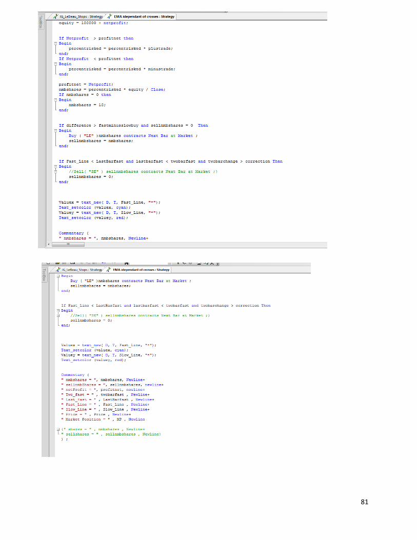
81
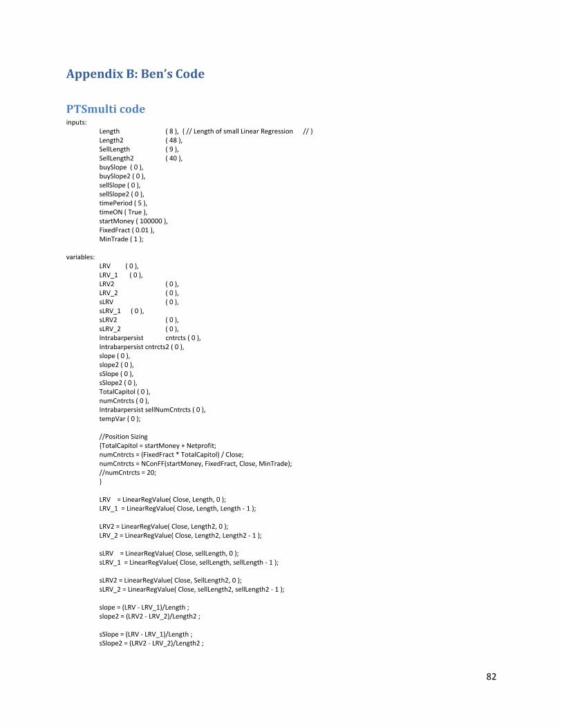
82
Appendix B: Ben’s Code
PTSmulti code inputs: Length ( 8 ), { // Length of small Linear Regression // } Length2 ( 48 ), SellLength ( 9 ), SellLength2 ( 40 ), buySlope ( 0 ), buySlope2 ( 0 ), sellSlope ( 0 ), sellSlope2 ( 0 ), timePeriod ( 5 ), timeON ( True ), startMoney ( 100000 ), FixedFract ( 0.01 ), MinTrade ( 1 ); variables: LRV ( 0 ), LRV_1 ( 0 ), LRV2 ( 0 ), LRV_2 ( 0 ), sLRV ( 0 ), sLRV_1 ( 0 ), sLRV2 ( 0 ), sLRV_2 ( 0 ), Intrabarpersist cntrcts ( 0 ), Intrabarpersist cntrcts2 ( 0 ), slope ( 0 ), slope2 ( 0 ), sSlope ( 0 ), sSlope2 ( 0 ), TotalCapitol ( 0 ), numCntrcts ( 0 ), Intrabarpersist sellNumCntrcts ( 0 ), tempVar ( 0 ); //Position Sizing {TotalCapitol = startMoney + Netprofit; numCntrcts = (FixedFract * TotalCapitol) / Close; numCntrcts = NConFF(startMoney, FixedFract, Close, MinTrade); //numCntrcts = 20; } LRV = LinearRegValue( Close, Length, 0 ); LRV_1 = LinearRegValue( Close, Length, Length - 1 ); LRV2 = LinearRegValue( Close, Length2, 0 ); LRV_2 = LinearRegValue( Close, Length2, Length2 - 1 ); sLRV = LinearRegValue( Close, sellLength, 0 ); sLRV_1 = LinearRegValue( Close, sellLength, sellLength - 1 ); sLRV2 = LinearRegValue( Close, SellLength2, 0 ); sLRV_2 = LinearRegValue( Close, sellLength2, sellLength2 - 1 ); slope = (LRV - LRV_1)/Length ; slope2 = (LRV2 - LRV_2)/Length2 ; sSlope = (LRV - LRV_1)/Length ; sSlope2 = (LRV2 - LRV_2)/Length2 ;

83
numCntrcts = 100; If Time > (930+ (timePeriod*Length)) and Time <= 1545 then Begin If slope > buySlope then Begin if tempVar = 0 and slope2 > buySlope2 then begin Buy ("Buy") numCntrcts contracts next bar at market; sellnumCntrcts = numCntrcts; tempVar = 1; end; end Else Begin Sell ("Sell") sellnumCntrcts contracts next bar at market; tempVar = 0; end; { If slope < sellSlope then Begin if tempVar = 0 then //and slope2 < sellSlope2 then begin Sellshort ("Short") numCntrcts contracts next bar at market; sellNumCntrcts = numCntrcts; tempVar = 1; end; end Else Begin Buytocover ("Cover") sellNumCntrcts contracts next bar at market; tempVar = 0;; end; } end Else if Time >= 1545 and timeOn then Begin Sell ("SellEnd") sellNumcntrcts contracts next bar at market; BuytoCover ("CoverEnd") sellNumcntrcts contracts next bar at market; tempVar = 0; end; {// Simplist form of strategy If slope > buySlope then Begin Buy ("Buy") 100 contracts next bar at market; end Else begin Sell ("Sell") 100 contracts next bar at market; end; } Commentary ( " Close: ", Close, " BuySlope: ", buySlope, " Slope: ", slope, " Time: ", time, " Gap: ", (930+ (5*Length))

84
);
PTStrending Code inputs: Length ( 27 ), //opt val { // Length of Linear Regression // } LengthS ( 27 ), Offset ( 1 ), BuyStop ( .13 ), buySlope ( 0 ), sellSlope ( 0 ), buyNum ( 0 ), sellNum ( 0 ), timeDisplay ( 75 ), { //75 for 20 min, 100 for 5 min, } BeginDate ( 0 ), { // Choose Zero to use full length // } BeginTime ( 0 ), { // Choose Zero to use full time // } EndDate ( 0 ), { // Choose Zero for Current Day // } EndTime ( 0 ), { // Choose Zero for Current Time // } NumDevsUp ( 1 ), { // Standard deviations for upper // } NumDevsDn ( -1 ), { // Standard deviations for lower // } NumDevsUpS ( 1 ), { // Standard deviations for upper // } NumDevsDnS ( -1 ), { // Standard deviations for lower // } LRColor ( Cyan ), { // Color for Linear Regression Line // } UBColor ( BLUE ), { // Color for Upper Boundary // } LBColor ( BLUE ); { // Color for Lower Boundary // } variables: VolumeValue ( 0 ), VolTotal ( 0 ), AvgVol ( 0 ), DayAvgVol ( 0 ), FirstDate ( 0 ), FirstTime ( 0 ), UpperBandS ( 0 ), LowerBandS ( 0 ), UpperBand_1S ( 0 ), LowerBand_1S ( 0 ), UpperBand ( 0 ), LowerBand ( 0 ), UpperBand_1 ( 0 ), LowerBand_1 ( 0 ), {UpperBand2 ( 0 ), LowerBand2 ( 0 ), UpperBand_2 ( 0 ), LowerBand_2 ( 0 ), UpperBand3 ( 0 ), LowerBand3 ( 0 ), UpperBand_3 ( 0 ), LowerBand_3 ( 0 ),} LRV ( 0 ), LRV_1 ( 0 ), SDev ( 0 ), LRVS ( 0 ), LRV_1S ( 0 ), SDevS ( 0 ), TL_LRV ( 0 ), TL_UB ( 0 ), TL_LB ( 0 ), TL_UB2 ( 0 ), TL_LB2 ( 0 ), TL_UB3 ( 0 ), TL_LB3 ( 0 ), cntrcts ( 0 ), slopeWasUp ( false ),

85
Intrabarpersist slope ( 0 ), prevSlope ( 0 ), ChngSlope( 0 ), tempBought ( 0 ); { Linear Regression Display } //gets starting date if BeginDate = 0 then FirstDate = date[ Length - 1 ] else FirstDate = BeginDate; //gets starting time if BeginTime = 0 then FirstTime = time[ Length - 1] else FirstTime = BeginTime; LRV = LinearRegValue( Close[Offset], Length, 0 ); LRV_1 = LinearRegValue( Close[Offset], Length, Length - 1 ); SDev = StandardDev( Close[Offset], Length, 1 ); LRVS = LinearRegValue( Close, Length, 0 ); LRV_1S = LinearRegValue( Close, Length, Length - 1); SDevS = StandardDev( Close, Length, 1); UpperBand = LRV + NumDevsUp * SDev; LowerBand = LRV + NumDevsDn * SDev; UpperBand_1 = LRV_1 + NumDevsUp * SDev; LowerBand_1 = LRV_1 + NumDevsDn * SDev; UpperBandS = LRVS + NumDevsUpS * SDevS; LowerBandS = LRVS + NumDevsDnS * SDevS; UpperBand_1S = LRV_1S + NumDevsUpS * SDevS; LowerBand_1S = LRV_1S + NumDevsDnS * SDevS; { UpperBand2 = LRV + NumDevsUp * 2*SDev; LowerBand2 = LRV + NumDevsDn * 2*SDev; UpperBand_2 = LRV_1 + NumDevsUp * 2*SDev; LowerBand_2 = LRV_1 + NumDevsDn * 2*SDev; UpperBand3 = LRV + NumDevsUp * 3*SDev; LowerBand3 = LRV + NumDevsDn * 3*SDev; UpperBand_3 = LRV_1 + NumDevsUp * 3*SDev; LowerBand_3 = LRV_1 + NumDevsDn * 3*SDev;} { The value of (LRV - LRV_1)/Length is the slope of the line Displays all of the slopes on the screen } if Mod(Time,timeDisplay)=0 then //If Date = 1130115 and Time = 1330 then Begin TL_LRV = TL_New( FirstDate, FirstTime, LRV_1, date, time, LRV ); TL_UB = TL_New( FirstDate, FirstTime, UpperBand_1, date, time, UpperBand ); TL_LB = TL_New( FirstDate, FirstTime, LowerBand_1, date, time, LowerBand ); { TL_UB2 = TL_New( FirstDate, FirstTime, UpperBand_2, date, time, UpperBand2 ); TL_LB2 = TL_New( FirstDate, FirstTime, LowerBand_2, date, time, LowerBand2 ); TL_UB3 = TL_New( FirstDate, FirstTime, UpperBand_3, date, time, UpperBand3 ); TL_LB3 = TL_New( FirstDate, FirstTime, LowerBand_3, date, time, LowerBand3 ); }

86
TL_SetColor( TL_LRV, LRColor ); TL_SetColor( TL_UB, UBColor ); TL_SetColor( TL_LB, LBColor ); { TL_SetColor( TL_UB2, RED); TL_SetColor( TL_LB2, RED); TL_SetColor( TL_UB3, Yellow); TL_SetColor( TL_LB3, Yellow); } TL_SetBegin( TL_LRV, FirstDate, FirstTime, LRV_1 ); TL_SetBegin( TL_UB, FirstDate, FirstTime, UpperBand_1 ); TL_SetBegin( TL_LB, FirstDate, FirstTime, LowerBand_1 ); { TL_SetBegin( TL_UB2, FirstDate, FirstTime, UpperBand_2 ); TL_SetBegin( TL_LB2, FirstDate, FirstTime, LowerBand_2 ); TL_SetBegin( TL_UB3, FirstDate, FirstTime, UpperBand_3 ); TL_SetBegin( TL_LB3, FirstDate, FirstTime, LowerBand_3 ); } TL_SetEnd( TL_LRV, date, time, LRV ); TL_SetEnd( TL_UB, date, time, UpperBand ); TL_SetEnd( TL_LB, date, time, LowerBand ); { TL_SetEnd( TL_UB2, date, time, UpperBand2 ); TL_SetEnd( TL_LB2, date, time, LowerBand2); TL_SetEnd( TL_UB3, date, time, UpperBand3 ); TL_SetEnd( TL_LB3, date, time, LowerBand3); } end; { LRV = LinearRegValue( Close, Length, 0 ); LRV_1 = LinearRegValue( Close, Length, Length - 1 ); SDev = StandardDev( Close, Length, 1 ); } prevSlope = slope; slope = (LRVS - LRV_1S)/Length ; ChngSlope = slope - prevSlope; If slope < sellSlope or Close < LRVS - SellNum then Begin If tempBought = 1 then Begin Sell ("Sell3rd") 100 contracts next bar at market; tempBought = 0; end; end; If Close > LRV + buyNum then Begin If tempBought = 0 then Begin Buy ("Buy") 100 contracts next bar at market; tempBought = 1; end; end; //Buy ("BuyStop") 1 contracts next bar at (High+BuyStop) stop; { If slope < sellSlope or Close < LowerBand2 then Begin
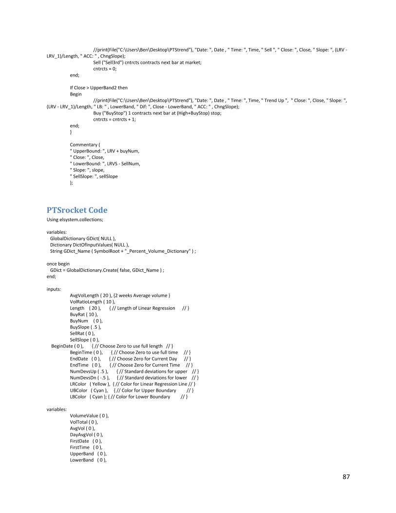
87
//print(File("C:\Users\Ben\Desktop\PTStrend"), "Date: ", Date , " Time: ", Time, " Sell ", " Close: ", Close, " Slope: ", (LRV - LRV_1)/Length, " ACC: " , ChngSlope); Sell ("Sell3rd") cntrcts contracts next bar at market; cntrcts = 0; end; If Close > UpperBand2 then Begin //print(File("C:\Users\Ben\Desktop\PTStrend"), "Date: ", Date , " Time: ", Time, " Trend Up ", " Close: ", Close, " Slope: ", (LRV - LRV_1)/Length, " LB: " , LowerBand, " Dif: ", Close - LowerBand, " ACC: " , ChngSlope); Buy ("BuyStop") 1 contracts next bar at (High+BuyStop) stop; cntrcts = cntrcts + 1; end; } Commentary ( " UpperBound: ", LRV + buyNum, " Close: ", Close, " LowerBound: ", LRVS - SellNum, " Slope: ", slope, " SellSlope: ", sellSlope );
PTSrocket Code Using elsystem.collections; variables: GlobalDictionary GDict( NULL ), Dictionary DictOfInputValues( NULL ), String GDict_Name ( SymbolRoot + "_Percent_Volume_Dictionary" ) ; once begin GDict = GlobalDictionary.Create( false, GDict_Name ) ; end; inputs: AvgVolLength ( 20 ), {2 weeks Average volume } VolRatioLength ( 10 ), Length ( 20 ), { // Length of Linear Regression // } BuyRat ( 10 ), BuyNum ( 0 ), BuySlope ( .5 ), SellRat ( 0 ), SellSlope ( 0 ), BeginDate ( 0 ), { // Choose Zero to use full length // } BeginTime ( 0 ), { // Choose Zero to use full time // } EndDate ( 0 ), { // Choose Zero for Current Day // } EndTime ( 0 ), { // Choose Zero for Current Time // } NumDevsUp ( .5 ), { // Standard deviations for upper // } NumDevsDn ( -.5 ), { // Standard deviations for lower // } LRColor ( Yellow ), { // Color for Linear Regression Line // } UBColor ( Cyan ), { // Color for Upper Boundary // } LBColor ( Cyan ); { // Color for Lower Boundary // } variables: VolumeValue ( 0 ), VolTotal ( 0 ), AvgVol ( 0 ), DayAvgVol ( 0 ), FirstDate ( 0 ), FirstTime ( 0 ), UpperBand ( 0 ), LowerBand ( 0 ),

88
UpperBand_1 ( 0 ), LowerBand_1 ( 0 ), LRV ( 0 ), LRV_1 ( 0 ), TL_LRV ( 0 ), TL_UB ( 0 ), TL_LB ( 0 ), SDev ( 0 ), Cts ( 0 ), ExpAv1(0), ExpAv2(0), longIn ( false ), shortIn ( False ), cntrcts ( 0 ), TotalTicks( 0 ), VolRatio( 0 ), VolRatioAvg( 0 ), tempBought ( 0 ), slope ( 0 ); { get global variables from other charts} If GDict.Contains( Date.toString() + "dayAvgVol2" ) then begin DayAvgVol = GDict[ Date.toString() + "dayAvgVol2" ] astype Double; end; {Average Volume Ratio (Up and Down) and Current Volume Ratio} {if Time > 1000 then begin } if BarType <= 1 or BarType >= 5 then begin TotalTicks = UpTicks + DownTicks ; if TotalTicks > 0 then VolRatio = 100 * ( UpTicks - DownTicks ) / TotalTicks else VolRatio = 0 ; VolRatioAvg = XAverage( VolRatio, VolRatioLength ) ; end; {End Else begin { need to figure out a way so that if a new day starts, it only looks at that day } VolRatio = 0; VolRatioAvg = 0; end; } {Average Volume and current Volume} if BarType >= 2 and BarType < 5 then begin VolumeValue = Volume ; AvgVol = AverageFC( Volume, AvgVolLength ) ; end else begin VolumeValue = Ticks ; AvgVol = AverageFC( Ticks, AvgVolLength ) ; end; { Linear Regression Display } //gets starting date if BeginDate = 0 then FirstDate = date[ Length - 1 ] else FirstDate = BeginDate;

89
//gets starting time if BeginTime = 0 then FirstTime = time[ Length - 1 ] else FirstTime = BeginTime; LRV = LinearRegValue( Close, Length, 0 ); LRV_1 = LinearRegValue( Close, Length, Length - 1 ); SDev = StandardDev( Close, Length, 1 ); UpperBand = LRV + NumDevsUp * SDev; LowerBand = LRV + NumDevsDn * SDev; UpperBand_1 = LRV_1 + NumDevsUp * SDev; LowerBand_1 = LRV_1 + NumDevsDn * SDev; slope = (LRV - LRV_1)/Length; {Strategy Two-VolumeRatio and Slope} if VolRatioAvg > BuyRat And Close > LRV + buyNum then // (was slope is within certain range, slope > BuySlope ), fuel is seen and breakthrough seen begin If tempBought = 0 then Begin Buy ("Buy2") 100 contracts next bar at market; tempBought = 1; end; end; if slope < SellSlope or VolRatioAvg < SellRat then //slope is going down or no fuel begin If tempBought = 1 then Begin Sell ("Sell2") 100 contracts next bar at market; tempBought = 0; end; end; {Strategy One-Volume and Slope} { if Volume/AvgVol > 1.6 then Begin if (LRV - LRV_1)/Length > 0 then Begin Buy ("Buy") 1 contracts next bar at market; print(File("C:\Users\Ben\Desktop\test2"), "Buy Slope: " , (LRV - LRV_1)/Length, " ratio: " , Volume/AvgVol); longIn = true; cntrcts = cntrcts + 1; End Else if (LRV - LRV_1)/Length < 0 then Begin Sellshort ("Short") 1 contracts next bar market; shortIn = true; cntrcts = cntrcts + 1; print(File("C:\Users\Ben\Desktop\test2"), "Short Slope: " , (LRV - LRV_1)/Length, " ratio: " , Volume/AvgVol); End; end; if shortIn And (LRV - LRV_1)/Length > 0 then Begin Buy to Cover ("Cover") cntrcts contracts next bar at market; print(File("C:\Users\Ben\Desktop\test2"), "Cover Slope: " , (LRV - LRV_1)/Length, " ratio: " , Volume/AvgVol); shortIn = false; end; If longIn And (LRV - LRV_1)/Length < 0 then Begin

90
Sell ("Sell") cntrcts contracts next bar at market; print(File("C:\Users\Ben\Desktop\test2"), "Sell Slope: " , (LRV - LRV_1)/Length, " ratio: " , Volume/AvgVol); longIn = false; End; }