i

Abstract

The pulsed plasma thruster (PPT) is an onboard electromagnetic propulsion device

currently being considered for use in various small satellite missions. The work

presented in this thesis is directed toward improving PPT performance using a control

engineering approach along with externally applied magnetic fields. An improved one

dimensional electromechanical model for PPT operation is developed. This slug model

represents the PPT as an LRC circuit with a dynamics equation for the ablated plasma.

The improved model includes detailed derivation for the induced magnetic field and a

model for the plasma resistance. A modified electromechanical model for the case of

externally applied magnetic fields is also derived for the parallel plate geometry. A

software package with a graphical user interface (GUI) is developed for the simulation of

various PPT types, geometric configurations, and parameters The simulations show

excellent agreement with data from the Lincoln Experimental Satellite (LES)-6, the LES-

8/9 PPT and the Univ. of Tokyo PPT. The control objective employed in this thesis

involves the maximization of the specific impulse and thrust efficiency of the PPT, which

are each directly related with the exhaust velocity of the thruster. This objective is

achieved through the use of an externally applied magnetic field as a system actuator. To

simulate an open-loop constant-input controller the modified electromechanical PPT

model is applied to the various PPT configurations. In this controller the external

magnetic field was applied as constant throughout or portions of the PPT channel. For

the Univ. of Tokyo PPT a magnetic field applied over the entire 6-cm long channel

increases the specific impulse and thrust efficiency by 10% over the case that the filed is

applied in the first 1.75 cm of the PPT channel. The magnitude of these increases

ii

compare well with the results of the UOT applied B-field experiments. For the LES-6

and LES-9 PPTs, the simulations predicts significant performance enhancements with

approximately linear increases for the specific impulse, thrust efficiency and impulse bit.

iii

Acknowledgements

The completion of this master’s thesis owes not only to my own effort, but to the help

and support of a number of individuals.

First of all, I would like to thank my future wife, Elizabeth Serrano, whose patience and

joy were the strength that brought this work to life.

I can’t thank the guys of CGPL enough for their friendship and camaraderie. Ryan,

Jimmy, Anton, you guys made my stay here at the lab that much more enjoyable and you

helped me in more ways than you know. You all are fantastic guys and I look forward to

what the future may have in store for us all.

I would also like to thank Professor Demetriou for the invaluable controls knowledge

ushered me into a new perspective in engineering. Additionally, I would be remiss not to

thank Professor Blandino for conducting the aerospace department group meetings.

Those meetings were instrumental in providing a forum with which to communicate my

ideas and work.

I also would like to thank the Massachusetts Space Grant Consortium for their financial

support of this work.

Most of all, I’d like to thank Professor Nikos Gatsonis, who taught me to communicate

engineering information more accurately and effectively and worked tirelessly to provide

me with every resource I requested (and then some). I am a much better engineer from

having been your student. Thanks.

iv

Table of Contents

Abstract ................................................................................................................................ i

Table of Contents............................................................................................................... iv

List of Figures .................................................................................................................... vi

Nomenclature...................................................................................................................... x

1. Introduction............................................................................................................. 1

1.1. Pulsed Plasma Thrusters and Microspacecraft ................................................ 1

1.2. Review of PPT Electromechanical Modeling................................................... 8 1.2.1. Parallel-Plate PPT ........................................................................................... 8 1.2.2. Coaxial PPT .................................................................................................. 13

1.3. Review of Applied Magnetic Field PPT......................................................... 18

1.4. Objectives and Approach............................................................................... 20

2. An Improved Electromechanical PPT Model ....................................................... 23

2.1. Introduction 23

2.2. Generalized Electromechanical Model for a Parallel-Plate PPT .................... 25 2.2.1. Parallel-Plate Self-Induced Magnetic Field .................................................. 26 2.2.2. Parallel-Plate Inductance Model ................................................................... 29 2.2.3. Mass Distribution Model .............................................................................. 30 2.2.4. Parallel-Plate Plasma Resistance Model....................................................... 31 2.2.5. Summary of the Parallel-Plate Electromechanical Model ............................ 34 a) Slug Operation .................................................................................................. 35 b) Snowplow Operation ............................................................................................ 37

2.2. Generalized Electromechanical Model for a Coaxial PPT ............................. 38 2.2.1. Coaxial Self-Induced Magnetic Field ........................................................... 39 2.2.2. Coaxial Electrode Inductance Model............................................................ 41 2.2.3. Coaxial Plasma Resistance Model ................................................................ 42 2.2.4. Summary of the Coaxial Electromechanical Model ..................................... 43 a) Slug Operation .................................................................................................. 44 b) Snowplow Operation ........................................................................................ 45

2.3. Electromechanical Model for an Applied Field PPT...................................... 45

v

3. Numerical Implementation, Software Implementation and Model Validation .... 51

3.1. Numerical Implementation ............................................................................. 51

3.2. Software Implementation................................................................................ 56

3.3. General Model Validation............................................................................... 58

3.4. Modified Model Validation ............................................................................ 62

4. Control Strategy and Analysis .............................................................................. 65

4.1. Control Objective and System ........................................................................ 65

4.2. Control Analysis ............................................................................................. 70 4.2.1. Reachability .................................................................................................. 72

5. Controller Simulations .......................................................................................... 75

5.1. 1984 UOT PPT ............................................................................................... 76

5.2. LES-6 .............................................................................................................. 78

5.3. LES-8/9 ........................................................................................................... 81

6. Conclusions and Recommendations ..................................................................... 84

6.1. Model Contributions, Analysis and Results.................................................... 84

6.2. Recommendations and Directions for Further Research ................................ 86

Appendix A. External Circuit Modified Models ............................................................. 88

References......................................................................................................................... 91

vi

List of Figures

Figure 1.1 Coaxial PPT cutaway. ...................................................................................... 4

Figure 1.2 Parallel plate PPT. ............................................................................................ 5

Figure 1.3 NASA GRC Laboratory PPT firing. ................................................................ 7

Figure 1.4 Parallel plate PPT components......................................................................... 9

Figure 1.5 Simplified electric circuit diagram. .................................................................. 9

Figure 1.6 Coaxial GFPPT Components ......................................................................... 14

Figure 1.7 PPT electric circuit diagram. .......................................................................... 14

Figure 2.1 PPT Types ...................................................................................................... 24

Figure 2.2 Parallel plate APPT. ....................................................................................... 25

Figure 2.3 Circuit model for parallel plate PPT............................................................... 25

Figure 2.4 Perfectly conducting one-turn solenoid.......................................................... 27

Figure 2.5 Ampere's Law applied throughout the current sheet ...................................... 28

Figure 2.6 Mass distribution function.............................................................................. 31

Figure 2.7 Plasma resistance model for LES-6 PPT........................................................ 33

Figure 2.8 Plasma resistance model for LES-8/9 PPT..................................................... 33

Figure 2.9 Coaxial GFPPT............................................................................................... 38

Figure 2.10 Circuit model of a coaxial PPT. ................................................................... 38

Figure 2.11 Coaxial PPT cutaway with uniform surface current..................................... 39

Figure 2.12 Coaxial Applied Magnetic Field PPT........................................................... 46

vii

Figure 3.1 General model simulation output using LES-6 thruster parameters. ............. 54

Figure 3.2 Nominal applied magnetic field PPT simulation (Bext =0.3 T)..................... 54

Figure 3.3 MATLAB® one dimensional PPT model GUI.............................................. 57

Figure 3.4 LES-6 circuit with voltage measurement. ...................................................... 59

Figure 3.5 LES-6 experiment and simulation comparison. ............................................. 60

Figure 3.6 LES-8/9 experiment and simulation comparison. .......................................... 61

Figure 3.7 Specific impulse and thrust efficiency validation comparison....................... 63

Figure 3.8 Impulse bit validation comparison. ................................................................ 63

Figure 4.1 Closed-loop and open-loop flow control........................................................ 65

Figure 4.2 Parallel plate PPT with external magnetic field applied via permanent

magnets. .................................................................................................................... 68

Figure 4.3 Open-loop controller using coupled external LCR circuit. ............................ 69

Figure 4.4 Closed-loop controller using coupled external circuit with voltage source. .. 70

Figure 5.1 1984 UOT PPT simulation current and distance (Bext = 0.3). ...................... 77

Figure 5.2 Specific impulse and thrust efficiency comparison........................................ 77

Figure 5.3 Impulse bit comparison. ................................................................................. 78

Figure 5.4 Effects of constant magnitude externally applied magnetic fields on current

sheet position and velocity for the LES-6................................................................. 79

Figure 5.5 Effects of constant magnitude externally applied magnetic fields on current

and capacitor voltage for the LES-6. ........................................................................ 80

Figure 5.6 Effects of accelerating magnetic fields on LES-6 performance. .................... 80

Figure 5.7 Effects of constant magnitude externally applied magnetic fields on current

sheet position and velocity for the LES-8/9.............................................................. 82

viii

Figure 5.8 Effects of constant magnitude externally applied magnetic fields on current

and capacitor voltage for the LES-8/9. ..................................................................... 82

Figure 5.9 Effects of accelerating magnetic fields on LES-8/9 performance.................. 83

ix

List of Tables

Table 1.1 UOT Applied Magnetic Field PPT Experimental Data ................................... 18

Table 3.1 General Model Validation ................................................................................ 58

Table 3.2 Experimental Parallel Plate PPT Data .............................................................. 58

Table 3.3 LES-6 simulation validation. ........................................................................... 61

Table 3.4 LES-8/9 simulation validation. ........................................................................ 62

x

Nomenclature

Symbol Definition ( SI Units )

A Current sheet cross sectional area (m2)

A Area vector (m2)

b Kinetic theory mass distribution coefficient (m-1)

0b Impact parameter (m)

B Total magnetic field vector (T)

extB Externally applied magnetic field (T)

indB Magnetic field vector due to PPT circuit self-inductance (T)

Bφ Azimuthal self-induced magnetic field (T)

fc Dynamic model damping term (N s m-1)

C Capacitance (F)

e Electron charge (C)

0E Energy stored on capacitor at 0t = (J)

cE Energy stored on capacitor (J)

BE Energy stored in magnetic field (J)

EΩ Energy dissipated in ohmic heating (J)

KEE Kinetic energy of current sheet (J)

f Drift vector field

F Total force vector acting on current sheet

indF Total Lorenz force due to self-inductance field (N)

LF Lorentz force (N)

g Acceleration due to gravity at sea level, 9.81 (m s-2)

xi

g Input vector field

g Photon momentum density (kg m s-1)

h Distance between electrodes in parallel plate geometry (m)

I Current (A)

bitI Impulse bit (N s)

spI Specific impulse (s)

j Current density field vector (A m-2)

k Boltzman constant, 1.3807e-23 (J K-1)

K Thermal conductivity of electron gas (W m-1 K-1)

K Surface current density vector (A m-1)

iK Surface current density (A m-1)

( )eKE Kinetic energy at exhaust (J)

l Channel length (m)

L Inductance (H)

0L Inductance at 0t = (H)

cL Internal inductance of the capacitor (H)

ceL Inductance due to current sheet moving down coaxial electrodes (H)

'ce

L Inductance per unit channel length for coaxial geometry (H m-1)

eL Inductance due to wires and leads (H)

peL Inductance due to current sheet moving down parallel plate electrodes (H)

'peL Inductance per unit channel length for parallel plate geometry (H m-1)

TL Total circuit inductance (H)

m Mass of current sheet (kg) 'm Mass per unit length (kg m-1)

0m Mass of current sheet at 0t = (kg)

em Mass of current sheet at exhaust (kg)

fm Propellant flow rate (kg s-1)

xii

im Ion mass (kg)

tm Total mass accumulated in current sheet during discharge (kg)

M Final spacecraft mass (kg)

0M Initial spacecraft mass (kg)

n Particle number density (m-3)

n Area normal vector

0n Neutral number density (m-3)

en Electron density (m-3)

p Particle momentum density (kg m s-1)

P Power delivered to circuit (J s-1)

fP Fraction of ionization and excitation accomplished at the expense of the

plasma thermal energy

P Particle stress tensor (N m-2)

Q Charge on capacitor (C)

r Radial distance (m)

ir Radius of inner electrode for coaxial geometry (m)

or Radius of outer electrode for coaxial geometry (m)

R Resistance (Ω)

0R Capacitor, wire and lead resistance (Ω)

cR Capacitor resistance (Ω)

eR Wire and lead resistance (Ω)

peR Electrode resistance (Ω)

pR Plasma resistance (Ω)

TR Total circuit resistance (Ω)

S Wall area (m2)

iS Electron-neutral collision term (m3 s-1)

t Time (s)

xiii

elt Electrode thickness for parallel plate geometry (m)

T Plasma temperature (K)

T Maxwell stress tensor (N m-2)

eT Electron temperature (K)

FT Thrust (N)

V Velocity (m s-1)

0V Voltage across capacitor at 0t = (V)

cV Voltage drop across capacitor (V)

w Width of electrodes in parallel plate geometry (m)

W Work (J)

1x Position state variable (m)

2x Charge on capacitor state variable (C)

3x Velocity state variable (m s-1)

4x Current state variable (A)

ex Current sheet exhaust velocity (m s-1)

sx Position vector of current sheet measured at the trailing edge of the current

sheet (m)

stx State vector

sx Position of current sheet measured at the trailing edge of the current sheet

(m)

z Charge number

α Mass distribution loading parameter

2α Two body recombination rate coefficient (m3 s-1)

3α Three body recombination rate coefficient (m6 s-1)

Γ Particle diffusion current (s-1)

δ Current sheet thickness (m)

xiv

tη Thrust efficiency

Λ Lamda parameter

PPTλ Total magnetic flux through PPT circuit (T m-2)

cλ Flux linkage through capacitor (T m-2)

eλ Flux linkage through wires and leads (T m-2)

peλ Flux linkage through the plate electrodes (T m-2)

Dλ Debye length (m)

yλ Total magnetic flux through magnetic yoke (T m-2)

0µ Magnetic permeability of free space, 1.2566e-6 (Wb A-1 m-1)

σ Conductivity (Ω-1 m-1)

pσ Plasma conductivity (Ω-1 m-1)

τ Characteristic pulse time (s)

1Φ Ionization-excitation potential per ion (V)

2Φ Excitation loss rate parameter (V s-1)

1

Chapter 1

Introduction 1. Introduction

1.1. Pulsed Plasma Thrusters and Microspacecraft

There is ongoing interest in the development of increasingly smaller, compact

satellites, in particular, for fleets or constellations of satellites to be used in current and

future missions. These missions, ranging from space-based interferometry to Department

of Defense radar and surveillance [Rayburn et al., 2005], could rely upon microspacecraft

with wet masses less than 100 kg [Mueller, 2000]. Evidence of microspacecraft interest

are the various programs that have been initiated by government and military institutions

intent on the development of microsatellite technology. The Air Force, for example, has

shown interest through its TechSat21 and University Nanosatellite Programs. The

TechSat21 program is intent on demonstrating the cost and functionality benefits of

replacing current large satellite system architecture with distributed networks of small

satellites [Cobb, 1999]. The University Nanosatellite program, has the goal of design,

fabrication and functional testing of small satellites [Campbell et al., 1999]. One of the

initial products of this program is the Ionospheric Observation Nanosatellite Formation

(ION-F). The operational goals of this three satellite formation are ionosphere science

measurements and a demonstration of formation flying [Campbell et al., 1999]. Integral

to the success of microsatellites flying in formation are the propulsion systems used to

maintain the relative positions of the spacecraft. In the case of the ION-F micro

2

satellites, an electric prolusion device, the micro pulsed plasma thruster (µPPT), with its

small discrete forces and overall fuel efficiency, was chosen to satisfy this requirement.

This device was chosen above other competing thrusters (e.g. cold gas thruster) due to

comparative mass savings benefits and its robust simplicity.

The significant advantages electric thrusters hold over their chemical counterparts

has led to such experiments as the Air Force Research Laboratory’s (AFRL) current

Microsatellite Propulsion Integration (MPI) mission. The objective of this experiment is

to “demonstrate greatly improved microsatellite maneuverability with low power electric

propulsion” [Johnson, et al., 2003]. It is certainly apparent from this abundance of

development and commitment that the market for electric propulsion, particularly for use

on small satellites, is on a continual rise.

The advantage electric propulsion has over chemical propulsion is a result of the

thrust production mechanism. Chemical propulsion relies solely upon gas dynamic

forces and effects for propellant acceleration. In contrast, electric propulsion

technologies, such as ion thrusters, Hall thrusters, colloid thrusters and pulsed plasma

thrusters (PPT), also have an electrostatic or an electromagnetic force component acting

on ionized propellant. The effective result of this difference is electric thrusters tend to

have exhaust velocities orders of magnitude greater than their chemical counterparts. A

quantification of the advantage of EP over chemical propulsion is found in the specific

impulse of the thrusters, defined as

.Fsp

f

TIm g

= (2.1)

where FT is the thrust, fm is the propellant mass flow rate and g is the acceleration of

gravity. While chemical thrusters have exhaust velocities and specific impulses upwards

3

of 4 km/s and 350 s, electric propulsion devices have exhaust velocities exceeding 30

km/s with specific impulses often greater than 1000 s. For given missions velocity

requirements, ,V∆ the “rocket equation” is

0ln ,spMV gIM

∆ =

(2.2)

where 0M is the initial spacecraft mass and M is the spacecraft mass after thruster

firing. Therefore, the increase in specific impulse results in less propellant mass being

needed for a given mission .V∆

While electric thrusters are more fuel efficient, this comes at an expense to the

instantaneous thrust level of these devices. Electric thrusters generate little more than a

few Newton’s of thrust, with many types of electric propulsion devices producing no

more than a few milli-Newton’s of thrust. Because of this, electric propulsion devices are

not suited for quick spacecraft maneuvers, such as orbit-raising on the order of hours or

days. However, for deep space exploration and a plethora of maneuvers; such as station

keeping, attitude control, slow orbit modifications and formation control, electric

thrusters continue to be the candidate of choice [Gagne, 2000].

Electric propulsion devices can be divided into several categories based on the

acceleration process involved: electrothermal, electrostatic, and electromagnetic. PPTs

are a form of electromagnetic propulsion, which has been in and around the industry

limelight for much of the history of electric propulsion. PPTs began to be developed

during the late 1950’s in facilities in Russia and the United States as a product of early

thermonuclear fusion experiments [Jahn et al., 2002]. Though PPT interest and

development reached a pinnacle in the mid 1960’s with several devices being flown on

4

spacecraft, by 1970 much of the early interest waned. In recent years, however, due to

the growing importance of small and micro-satellites, a renewed interest in PPTs has

arisen.

There are several types of PPTs currently under investigation. They are

categorized by the geometry of the electrodes and the propellant being utilized. The

electrode configurations are coaxial (Figure 1.1) or parallel plate (Figure 1.2) and the

propellants are gas or ablated solid.

Figure 1.1 Coaxial PPT cutaway.

5

Figure 1.2 Parallel plate PPT.

The gas-fed PPT (GFPPT) utilizes a gas for propellant, with the noble gasses (e.g.

xenon and argon) most often being used. It consists of a gas storage device, a gas inlet,

two electrodes spaced to form a channel, a sparking device and a main energy storage

capacitor. Historically, GFPPT required the use of fast acting valves; however, recent

developments of pulsing schemes for GFPPT have eliminated this need [Ziemer et al.,

1997]. The sparking device is embedded in one of the plates as a means to initiate the

gas ionization. Once an initial ionization is accomplished the main capacitor is

discharged across the electrodes. This creates an approximately axially symmetric

current sheet at the surface of the insulator. With current flowing through the complete

PPT circuit, a self-magnetic field is produced. This magnetic field interacts with the

current sheet by accelerating it through a ×j B Lorentz force. The direction of this force

is to increase the area of the PPT circuit loop. This electromagnetic force coupled with

gas dynamic forces act to accelerate the relatively dense current sheet entraining the

neutral gas further up the channel as it exits the thruster.

6

An ablative PPT utilizes a solid (generally Teflon) for propellant. It consists of a

spring fed piece of Teflon at the back a thruster channel, the two electrodes that form the

channel, a sparking device and a main energy storage capacitor. The sparking device is

located at the back of the thruster channel ensuring the creation of a current sheet along

the Teflon face. Once the sparking device is fired, the main capacitor is discharged. The

thermal flux and particle bombardment from the current ablates and ionizes a small

amount of the solid. With current flowing through the complete PPT circuit, a self-

magnetic field is produced. This magnetic field interacts with the current sheet by a

×j B Lorentz force as to increase the area PPT circuit loop. This force coupled with the

gas dynamic expansion forces accelerate the current sheet out of the thruster at velocities

upwards of 40 km/s [Vondra, 1970].

The beginnings of the PPT can be traced back to thermonuclear fusion programs

conducted in the United States and Russia during the 1950s. A derivative of these

programs was a family of plasma accelerators closely related to the GFPPT [Jahn et al.,

2002]. With these accelerators being modified for propulsion configuration, by the early

1960s both Russia and the United States had developed the first PPT systems [Jahn et al.,

2002]. The first flight-tested electric propulsion device was a Russian PPT flown on the

Zond-2 spacecraft in 1964 providing three-axis attitude control [Pollard et al, 1993]. For

several years after this first flight, development and testing continued in both Russia and

the United States resulting in the United States successfully flying PPTs on the LES-6

satellite for station keeping purposes. This early PPT work also resulted in several other

PPT thruster, notably the LES-8/9. Figure 1.3 shows a recent derivative of the LES-8/9,

the NASA Goddard Research Center (GRC) Laboratory PPT. This laboratory PPT was

7

utilized in experimental and modeling investigation as summarized in Gatsonis et al

(2001).

Figure 1.3 NASA GRC Laboratory PPT firing.

Despite the early successes with providing secondary propulsion, the majority of

the electric propulsion research throughout the 1970s was directed at producing primary

propulsion systems for large satellites. With only GFPPTs able provide the required level

of thrusting, PPT researchers ran into engineering limitations. These limitations were

with the massive capacitors and the lifetime requirements of fast-acting valves needed to

achieve high propellant mass utilization. As a result of these issues, by 1975, research

and development of GFPPTs waned [Pollard et al., 1993]. PPT research did continue on

at much diminished rate as the APPT was utilized as a secondary propulsion system on a

series of U.S. Navy satellites and in several experiments independently conducted by

China and the United States [Jahn et al., 2002].

Despite these flights, PPT research remained relatively dormant until the mid-

1990s when the development of power-limited satellites was initiated by an interest in

formations and constellations of small satellites. With improved capacitor technology,

the APPT was looked upon as a leading contender for a plethora of attitude control and

station keeping maneuvers on these low power satellites. This rekindled APPT

8

development has also sparked renewed interest in the GFPPT. Recent developments in

pulsing schemes have eliminated the need for fast-acting valves in GFPPTs. These recent

developments have once again brought the PPT back into the limelight of spacecraft

technology.

1.2. Review of PPT Electromechanical Modeling

Much research has been conducted at various industrial and academic facilities to

improve the design and performance characteristics of the PPT. In particular, a

significant amount of theoretical modeling has been performed ranging from low-order

one dimensional models [Jahn, 1968] to advanced MHD modeling [Mikellides, 1998].

This section specifically addresses the low-order slug/snowplow modeling that has been

performed. In the modeling review, the various one-dimensional electromechanical

models that have been derived and employed in the analysis and optimization of parallel-

plate and coaxial PPTs are addressed. These models are listed chronologically; however,

due to the great amount of previous work performed in this area, only models containing

unique advances over previous modeling efforts are listed.

1.2.1. Parallel-Plate PPT

The development of a simple one-dimensional mathematical model of parallel

plate PPT operation first appears in Jahn [1968]. It appears along with several other

heuristic models aimed at describing unsteady electromagnetic acceleration. In this

model the acceleration process and circuit components of the PPT are modeled as a

dynamical system interacting with an electrical system, that is, as an electromechanical

system.

9

Figure 1.4 Parallel plate PPT components.

The parallel plate PPT (shown in Figure 1.4) operates electrically as an LRC

circuit (Figure 1.5).

Figure 1.5 Simplified electric circuit diagram.

Accordingly, Jahn modeled the electrical system with the following circuit equation

( ) ( ) ( )'0 0

0

1 0.t

c pe sd dV LI RI V I d L L x I RIdt C dt

τ τ + + = − + + + = ∫ (2.3)

where '0 0, , , , , , , and c pe sV L I V C L L x R are, respectively, the voltage across the

capacitor, total circuit inductance, circuit current, initial voltage, capacitance, initial

inductance, inductance per unit length for parallel plate electrodes, current sheet position

10

(measured at the trailing edge of the current sheet) and circuit resistance. This equation is

a statement of Kirchoff’s voltage law for the circuit appearing in Fig 1.5. By

approximating the parallel plates as quasi-infinite in width ( ) ,w h>> the parallel plate

inductance per unit length, ' ,peL can be written as

'0 ,pe

hLw

µ= (2.4)

where 0, and h w µ are, respectively, the distance between parallel plate electrodes, the

width of the electrodes and the magnetic permeability. Though the resistance of the

plasma, ,pR may be time varying in an unknown manner, Jahn lumped it into a constant

circuit resistance term .R Dynamically, the entire mass in the current sheet was

presumed to be accelerated as a single unit or “slug”. Under this assumption, Jahn

represented the dynamical system of his PPT model through Newton’s Second Law as

( ) ' 21 ,2s pe

d mx L Idt

= (2.5)

where 0 ,m m= the mass of the current sheet, is taken as being constant throughout the

process. The term on the right corresponds to the ×j B electromagnetic force acting on

the current sheet. In this model the gas dynamic forces acting on the current sheet are

presumed to be negligible.

The slug model was used extensively in the investigation of the Lincoln

Laboratories LES family of parallel plate PPTs beginning with Waltz [1969] and the

LES-6 thruster. The equations in Waltz remain unchanged from Jahn’s model with the

exception that the conservation of energy for the circuit was utilized instead of the circuit

equation (Kirchoff’s voltage law). The conservation of energy for the system was found

11

by expanding the circuit equation, multiplying each term in the circuit equation by

I CV= − and integrating it with respect to time

( ) ( )' 2 2 ' 2 20 0 0

0 0

1 1 1 1 ,2 2 2 2

t t

pe s c pe pL L x I CV L Id R R I d CVτ τ+ + + + + =∫ ∫ (2.6)

where 0R is the resistance due to the capacitor, wires and leads and pR is the plasma

resistance. The terms in (2.6) represent, respectively, the energy stored in the magnetic

field, the capacitor energy, the kinetic energy supplied to the slug, ohmic heating losses

and the total energy for the system.

An improved electromechanical model appeared in Vondra [1970] in an attempt

to improve the LES-6 design. While the circuit equation of this slug model remained

unchanged, Vondra made a significant change to the dynamical equation, writing the

momentum balance in terms of the Maxwell stress tensor ,T the particle stress tensor ,P

the particle momentum density ,p and photon momentum density .g Here, the

divergence of the Maxwell stress tensor gives the particle electromagnetic force density

and the divergence of the particle stress tensor gives the gas dynamic force density.

These are related to the particle momentum density and the photon momentum density

through the following momentum equation,

( ) ( ) 0.T P dV p g dVt∂

∇ ⋅ + + + =∂∫∫∫ ∫∫∫ (2.7)

This equation was simplified through various assumptions and calculus manipulation to,

' 20

0

1 ,2

t

pe sL I hwnkT dt m x + = ∫ (2.8)

whose time derivative is

12

( ) ' 20

1 ,2s pe

d m x L I hwnkTdt

= + (2.9)

where k is Boltzman’s constant, n is the particle number density and T is the plasma

temperature. In comparing this equation with previous models it is seen that there is an

extra force term acting on the slug. This force models the gas dynamic forces

accelerating the slug away from the Teflon face.

The next appearance of a parallel plate APPT slug model was in a thesis aimed at

optimizing the LES-8/9 APPT [Leiweke, 1996]. This model is identical to Waltz except

that two different inductance models were analyzed. In addition to the original

inductance model run in previous work, a specialized “fringe” inductance model was

developed. The original model approximated the system by assuming quasi-infinite

parallel plate geometry. “Fringe” effects are those effects due to finite parallel plate

geometry. The “fringe” inductance model attempted to model these effects under the

premise that parallel plate geometries made these effects non-negligible. However, after

comparing the results of each model to real LES data it was found that the original

inductance model produced more accurate results.

Another attempt to improve on the inductance model was presented by Burton et

al [1998]. This model incorporates finite-width and non-zero plate thickness effects of

real rectangular parallel plate conductors

( )0 3 ln 0.22 ,2pe s s el

el

hL x x h w tw t

µπ

= + − + + +

(2.10)

where elt is the plate thickness. Differentiating (2.10) with respect to the current sheet

position leads to an inductance per unit length down the channel of the PPT given by

13

' 0 3 ln .2pe

el

hLw t

µπ

= + +

(2.11)

The most recent modification to the parallel plate slug model appears in a paper

by Gatsonis and Demetriou [2004]. This work is the first attempt of its kind at utilizing

the slug model to develop a feedback controller aimed at optimizing the exhaust velocity

of the PPT. The regular integro-differential system of equations is utilized in this model,

with the notable exception of damping and control terms being added in the momentum

equation. The control term here is assumed to be an externally applied magnetic field,

( ) ' 21 ,2s pe ext f s

d mx L I IhB c xdt

= + − (2.12)

where extB and fc are, respectively, the external field strength and frictional damping

coefficient.

1.2.2. Coaxial PPT

The majority of one-dimensional PPT modeling throughout the last 40 years has

been developed for coaxial GFPPTs (Figure 2.3). The geometric and operational

differences of these thrusters with ablative PPTs call for different one-dimensional

models than those utilized in the previously discussed parallel plate PPTs. The

appearance of a simple one-dimensional mathematical model of coaxial GFPPT operation

first appears in Hart [1962] seven years before the first parallel plate PPT model. Hart

developed this model to describe the operating conditions of a predecessor of the coaxial

GFPPT; the gas-fed plasma gun.

14

Figure 1.6 Coaxial GFPPT Components

This model constitutes the first known appearance of the snowplow model in literature.

At first glance there is very little difference between this model and the simple slug

models previously discussed. As for the slug models, Hart’s snowplow model was a

dynamical system interacting with an electrical system. The electrical system was

modeled as an LRC circuit, shown in Figure 2.4, exactly as it was for the parallel plate

PPT with no differences.

Figure 1.7 PPT electric circuit diagram.

Kirchhov’s voltage law applied across this circuit yields the circuit equation,

( ) ( ) ( )'0 0 0

0

1 0,t

ce s pdV I d L L x I R R I

C dtτ τ − + + + + = ∫ (2.13)

with 'ceL being the inductance per unit coaxial electrode length, given by

15

' 2 ln ,oce

i

rLr

=

(2.14)

where or and ir are, respectively, the outer and inner electrode radii.

For the dynamical system, the current sheet was modeled as an initial mass, 0 ,m

being accelerated electromagnetically down the channel gap with a distribution of gas

throughout the channel. The snowplow model diverges from the slug model at this point

with initial current sheet mass “sweeping up” this downstream mass as it accelerates

down the channel. This current sheet effectively acts as a piston as it travels out of the

thruster.

Just as in the previous parallel plate models, the two systems (electrical and

dynamical) were connected by equating the change in momentum of the current sheet to

the impulse acting on it. The force acting on the current sheet “piston” due to the Lorentz

force acting on it was modeled as before

2'12

.L ceF L I= (2.15)

Thus, Newton’s second law of motion for the system is,

( ) ' 212s cemx L

d Idt

= (2.16)

where ( )0'

sm m xm += and 'm was the mass per unit channel length.

Michels et al. (1966) developed a highly modified version of Hart’s snowplow

model. One major adaptation allowed for a variable initial mass-loading distribution.

This allowed for a gas distribution over the range between constant mass distributions

16

over the channel ( )1α = to the slug model case with all mass located at the back of the

thruster channel ( )0α =

1

1

0 1 1 ,sxm ml

α−

= − −

(2.17).

where and lα are, respectively, the mass loading parameter and the channel length.

Additionally, this model incorporated the effect of wall drag, ionization, and radiation

losses through an additional variable, the plasma temperature, .T With three unknowns,

this model is described by a coupled, three integro-differential equation system. These

three equations are the circuit equation (Kirchhoff’s Law), the momentum equation, and

the plasma energy equation. The circuit equation for the system was derived by

differentiating the circuit-energy equation and dividing by ,I

( ) ( ) ( ) ( )'0

0

1 t

ce sdI d L L x t I t RI t

C dtτ τ = + + + ∫

( ) ( ) ( ) ( ) ( )

1 21 1 .

i i

m t m tdP T TI t dt m m

− Φ +Γ + Φ

(2.18)

The terms 1 2, , , and im PΓ Φ Φ appearing in this equation are, respectively, the particle

diffusion current, ionization-excitation potential per ion, the excitation loss rate

parameter, the average ion mass and the fraction of ionization and excitation

accomplished at the expense of the plasma thermal energy. This circuit equation

includes terms for electrical energy lost by radiation and absorbed in both ionizing and

exciting particles swept up by the current sheet and in re-ionizing and re-exciting

particles that have diffused to the walls. The momentum equation had only one extra

17

term, which removes the forward momentum of every particle which strikes the wall.

Therefore, the equation of motion was given as

( ) ( ) ( ) ( )2'1 .2s ce i s

d mx t L I t m T x tdt

= − Γ (2.19)

The plasma energy equation is the most significant addition to the simple snowplow

model. It includes two heating sources, ohmic heating and the rate of heating due to

thermalization of kinetic energy. On the other hand, the equation includes four energy

loss terms. These are the losses associated with particle diffusion, ionization and

excitation losses, losses due to conduction of heat energy in the electron gas and

convective losses associated with the main electron conduction current. Accordingly, the

plasma energy equation is as follows,

( ) ( ) ( ) ( ) ( ) ( ) ( )2 2 23 1 31 12 2 2p s s

i

m td kT z R I t m x t kT z T x tdt m

+ = + − + Γ −

( ) ( ) ( ) ( ) ( )1 23 ,2i i wall

Im t m tP T T K T dS kT

m m e Φ +Γ + Φ − − ∇ −

∫ (2.20)

where , and K z e are, respectively, the thermal conductivity of the electron gas, the

average ion charge and the charge of an electron. Michels’ model is by far the most

advanced snowplow model published, in that it attempts to model many of the physical

phenomena that are occurring in the GFPPT. Models appearing after Michels’ model are

all the simple snowplow type like Hart’s. The only noteworthy exception to this was in

Ziemer and Choueiri’s [1998] coaxial GFPPT model. In this model the mass distribution

equation is derived from a one-dimensional kinetic theory description of a gas column

expanding out into a vacuum.

18

( )( ) 2

2*

' *0

0

sx t xbm t m m e dx

−= + ∫ (2.21)

1.3. Review of Applied Magnetic Field PPT

The first applied magnetic field study was performed by a group at the University

of Tokyo (UOT) during the years of 1976-1984. Over the course of these eight years,

three publications were released detailing the experimental investigations of a number of

thruster and applied field configurations (Table 2.1)

Table 1.1 UOT Applied Magnetic Field PPT Experimental Data

Publication Year 1978 1979 1984 Geometry Coaxial Parallel Plate Parallel Plate

Straight Parallel Plate

Flared Parallel Plate

Straight Inner Radius (cm) 0.4 - - - - Outer Radius (cm) 2.0 - - - - Gap Width (cm) - 1.8 4.0 4.0-6.0 4.0 5.0 Plate Width (cm) - 1.2 1.2 1.2-4.0 1.2

Channel Length (cm) 1.0 5.5 5.5 5.5 6.0 Initial Voltage (V) 1350-2300 1000-1500 2500 2500 2500 Capacitance (µF) 400 5.1 4.7 10 4.7 10 40

Initial Inductance (nH) 1500 -- 65 250 65 250 120 Mass Bit (µg) 130-530 6-18 10-55 5-55 60-320

External Field Type Axial Diverging

Accelerating Accelerating/ Retarding

Accelerating/ Retarding

Accelerating

Field Mechanism Electro Electro Electro/ Permanent

Electro/ Permanent

Permanent

In the preliminary experiments, electromagnets were applied to both coaxial and

parallel plate thruster geometries [Kimura et al., 1978]. In the case of the coaxial

geometry the applied magnetic field was axially diverging applied by a pulse-forming

network connected to a coil of wire wound around the outside of the outer electrode.

Two variations of this geometry were tested, one with the cathode as the inner electrode

and the other with the cathode as the outer electrode. While the results for both coaxial

variations showed improvements over nominal operation, with up to a 50% increase in

impulse bit with a 0.5 T external field, the parallel plate experiments showed significantly

19

better results. In the parallel plate case, the external magnetic field was applied

orthogonal to the current sheet in a direction that would produce an accelerating Lorentz

force for the first half wavelength of the capacitor discharge. This accelerating field was

applied by two magnetic coils, one on each side of the thruster channel, connected to a

pulse forming network. The results for impulse bit showed a 100% increase over the

nominal value, at an applied magnetic of only 0.2 T.

With this encouraging parallel plate result, the group shifted their applied

magnetic field investigation toward this geometry. In their next published work, both

electromagnets and permanent magnets were utilized in producing accelerating and

retarding external magnetic fields in parallel plate PPTs [Kimura, 1979]. The results for

this extensive investigation were slightly different than the preliminary investigation. For

the case of an accelerating external magnetic field, the impulse bit was found to initially

drop with an increase in applied magnetic field and then slowly increase thereafter. The

opposite was found to be the case for a retarding external magnetic field. For these

fields, there is an initial increase in impulse bit with magnetic field, then a slight decrease

thereafter. This result, when taken with the mass bit data, indicated that an applied

magnetic field could be used to change the thruster acceleration mechanism. A retarding

magnetic field was found to cause the thruster to operate predominately gas dynamically,

while an accelerating field causes the electromagnetic Lorentz force to predominate. The

specific impulse data for each applied field confirms this conclusion. For a retarding

field the specific impulse decreases with field strength with the opposite happening for an

accelerating magnetic field. In the case of the accelerating external field, at a field

strength of 0.35 T, the specific impulse increased at a rate as high as 2500 s per Tesla, the

20

thrust efficiency increased around 15 % per Tesla. The maximum decrease in impulse bit

for an accelerating field was around 30% and occurred at 0.1 T.

In their last work with accelerating magnetic fields, the Japanese group examined

the effects of accelerating magnetic fields in a single parallel plate geometry [Takegahara

et al., 1984]. Additionally, in this work, it appears that the mechanism for magnetic field

application was permanent magnets. The improvements in this case, were similar in

magnitude to the previous experiments, with an increase in specific impulse at a rate of

and 9000 s per Tesla and an increase in thrust efficiency of 30% per Tesla. The impulse

bit, in this case, exhibited a much more significant drop around 50% of its nominal value

at a field strength of 0.3 T.

After their 1984 work, the UOT group, for reasons unknown, abandoned their

pursuit of applied magnetic field PPTs and for 18 years the idea lay relatively dormant.

Only recently, in work here at WPI, have applied magnetic field PPTs been reexamined

[Gatsonis et al, 2004]. This modeling work addresses applied magnetic field PPTs from a

control engineering perspective by utilizing the fields as an actuator in the PPT system.

A closed-loop feedback controller was designed and simulated through an

electromechanical slug model. The feedback controller simulations presented in this

paper were shown to increase performance of the PPT through an increase in exhaust

velocity over the case of no control.

1.4. Objectives and Approach

With the recent interests in PPTs, research and investigations throughout industry

and academia have been numerous. Much of this effort has been conducted to optimize

thruster performance through a better understanding of the fundamental plasma dynamics

21

in the plume and electrode regions of the thruster. Despite this increase in research, the

prospect of using flow control engineering for PPT optimization has not been recently

addressed. This lack of control engineering is also the case for most other electric

propulsion devices. Flow control involves taking a flow system that has a set of inputs

and outputs (e.g. voltage, velocity, current, etc.) and manipulating the inputs to realize a

specific desired output. This type of control could be utilized to optimize such PPT

system performance parameters as the specific impulse and impulse bit using inputs such

as an external magnetic field.

This thesis is aimed at exploring the possibility of using flow-control for PPT

performance optimization. The introduction presents the PPT with its various types and

geometric configurations and discusses its accompanying history.

Objectives and Approach:

• Develop an improved electromechanical model for the parallel-plate PPT.

• Develop a software package modeling a general PPT with a graphical user interface

(GUI) to simulate various PPT types, geometric configurations, and parameters.

• Develop an electromechanical model modified to include externally applied magnetic

field effects.

• Using this modified model, examine the effects of externally applied magnetic fields

on PPT performance.

• Propose and design an open-loop controller to optimize the specific impulse and

thrust efficiency of a PPT.

The choice of one dimensional PPT plasma flow models is critical in this control

study and so a review of previously published models appearing over the last 40 years is

22

presented in chapter two. This chapter also details the equally important externally

applied magnetic field work performed at the University of Tokyo (UOT). Chapter three

presents the general one-dimensional PPT model and the modified version of this model

that includes applied magnetic field effects. Chapter four discusses the numerical scheme

employed in solving this model and details the GUI implemented for the general model.

Additionally, both the general and modified models are validated in this chapter. Chapter

five presents the control strategy and controller that were utilized in this study and

presents a brief control analysis of the modified model system. Chapter six presents the

simulation of the controller in various PPTs determining its effects on thruster

performance. Chapter seven presents the overall conclusions, addressing the results and

contributions of this work, and gives recommendations for future research.

23

Chapter 2

An Improved Electromechanical PPT

Model 2. An Improved Electromechanical PPT Model

2.1. Introduction

A low-order dynamical model is used to describe the current sheet motion in rectangular

and coaxial PPT geometries. Slug and snowplow models were chosen to accomplish this

due to their simplicity and proven accuracy. Furthermore, their simplicity warrant use as

tools for developing a control strategy for PPT operation. This strategy was implemented

and investigated by the use of a version of these models modified to include externally

applied magnetic field effects.

The basis of the one dimensional PPT model is to approximate the PPT system as

an electromechanical device with an electrical circuit interacting with a dynamical

system. The electric circuit is theoretically idealized in both models as a LCR circuit

with discrete, albeit moveable, elements. The physical law which is used to describe the

dynamics of the circuit is Kirchoff’s voltage law, which is itself derived from Maxwell’s

charge continuity equation for the circuit. In general, the inductance and current are

functions of time with all other parameters, including resistance, remaining constant over

the acceleration process. The dynamical system is idealized as an initial mass of plasma

being accelerated by a Lorentz ×j B force out of the thruster. Accordingly, the physical

24

law used to describe the situation is Newton’s second law of motion. The difference

between the slug and snowplow variations of the model is in the mass of the current

sheet. In the slug model, the initial mass is constant throughout the entire process. On

the other hand, in the snowplow model, the initial mass of plasma entrains additional

ambient gas mass as it propagates out of the thruster.

This chapter includes the derivations of both the general models for parallel plate

and coaxial PPT geometries as well as a modified model for the parallel plate geometry.

The derivation includes details of the self-induced magnetic field, the inductance model,

the plasma resistance model and the mass distribution model utilized for each geometry.

Beside the electrode geometry, PPTs are further classified as either ablative or gas-fed

based on the propellant utilized (Figure 2.1).

Parallel Plate Ablative PPT Coaxial Ablative PPT

Parallel Plate GFPPT Coaxial GFPPT

Figure 2.1 PPT Types

Variations of the electromechanical model specifically addressing these operating

regimes are presented for each geometry. Though not commonly investigated, the

parallel-plate GFPPT was modeled in this study, due in part to the recent experiments of

25

Ziemer et al. (1999 and 2000) examining these thrusters from an experimental

perspective. Generally, ablative PPTs have a constant mass bit equal to the initial mass,

0 ,m however, for side-fed ablative thrusters, the current sheet mass will increase as it

traverses down the channel, 0.tm ≠ This configuration can be simulated through

applying the snowplow model.

2.2. Generalized Electromechanical Model for a Parallel-Plate PPT

Figure 2.2 Parallel plate APPT.

The parallel plate PPT thruster, shown in Figure 2.2, with the moving discharge,

is described electrically as an LCR circuit as in Figure 2.3.

Figure 2.3 Circuit model for parallel plate PPT.

26

The inductance terms , and c pe eL L L are due, respectively, to the capacitor, the plate

electrode geometry and the wires and leads. The resistance terms , , and c e pe pR R R R are

due, respectively, to the capacitor, the wires and leads, the plate electrodes and the

plasma. Applying Faraday’s law around the circuit depicted in Figure 3.2 yields

( ) ( ) ( ) ,C T PPTdV t IR t tdt

λ = + (2.1)

where ( ) ( )T c e pe pR t R R R R t= + + + and ( )PPT tλ is the total flux linkage through the

PPT circuit. The flux linkage can be written in terms of the components of the PPT as

( ) ( ) ( ) ( ) ,PPT c e pet t t tλ λ λ λ= + + (2.2)

where the three terms on the right are, respectively, the magnetic flux due to the capacitor

inductance, the wire and lead inductance and the flux through the plate electrode channel.

Rewriting (2.2) in terms of the capacitor and wire and lead self-inductances yields

( ) ( ) ( ) ( ), ,PPT c e indelectrodes

t L I t L I t x y dλ = + + ⋅∫∫ B A (2.3)

where ,cL ,eL indB and A are, respectively, the capacitor self-inductance, the wire and

lead self-inductance, the self-induced field throughout the current sheet and an area

vector.

2.2.1. Parallel-Plate Self-Induced Magnetic Field

The magnetic field behind the current sheet is found by first assuming the

parallel-plate geometry can be approximated as quasi-infinite width, one-turn solenoid

composed of perfectly conducting sheets (Figure 2.4).

27

Figure 2.4 Perfectly conducting one-turn solenoid

Other than perfect conduction, this approximation also assumes that that each sheet has a

uniform current per unit width, K and that w h . These simplifications contrast with a

real parallel-plate PPT in the following ways. First, though the electrodes will have a

very high conductivity, which can be quite accurately approximated as infinite, the

plasma current sheet will have a finite conductivity. This finite plasma conductivity will

also lend to the current sheet having a thickness, ,δ in contrast to the sheet assumption.

Finally, most parallel plate geometries have that ,h w> and are expected to exhibit fringe

effects in contrast to the one-turn solenoid approximation.

The magnetic field contained within the one-turn solenoid will satisfy Ampere’s

continuity condition with the following boundary conditions on the perfect conductor

[Haus et al., 1989, pp 335]

0

0,ind

µ⋅ =Bn (2.4)

0

,ind

µ× =

Bn K (2.5)

where n is the normal area vector and K is the current per unit width vector. This gives

the magnetic field inside of the quasi-infinite width, one turn solenoid as

28

0 0ˆ ˆindIKw

µ µ= =B y y (2.6)

The magnetic field throughout the current sheet can be found by applying Ampere’s Law

to a surface S passing through the current sheet and using the magnetic field inside the

solenoid (2.6) as a boundary condition (Figure 2.5).

Figure 2.5 Ampere's Law applied throughout the current sheet

If the current density throughout the sheet is uniform and equal to

( ) ( ) ˆ,I t

twδ

= −j z (2.7)

then the magnetic field throughout the sheet will be given by,

( ) ( ) ( )0 ˆ, 1 .s

ind

I t x x tx t

wµ

δ −

= −

B y (2.8)

The magnetic field in front of the current sheet can be found similarly and is equal to

zero. Therefore, taking (2.6) and (2.8) together with zero field ahead of the current sheet

gives the full description of the magnetic field used in this model

29

( )

( ) ( )

( ) ( ) ( ) ( )

( )

0

0

ˆ , 0

ˆ, 1 , .

0,

s

sind s s

s

I tx x t

wI t x x t

x t x t x x tw

x x t

µ

µ δδ

δ

< <

−= − < < +

> +

y

B y (2.9)

2.2.2. Parallel-Plate Inductance Model

Going back the equation (2.3) and substituting the plate electrode magnetic field

(2.9) yields

( ) ( ) ( ) ( )( ) ( ) ( )( )

( )

0 00 0 0

1 .s s

s

x t x th hs

PPT c ex t

I t I t x x tt L I t L I t dydx dydx

w w

δ

λ µ µδ

+ −= + + + −

∫ ∫ ∫ ∫ (2.10)

Integrating the later two terms yields

( ) ( ) ( ) ( ) ( )0 0 .2PPT c e s

h ht L I t L I t x t I tw w

δλ µ µ = + + + (2.11)

The term in brackets in equation (2.11) is the self-inductance due to parallel-plate

electrodes,

( )( ) ( )( )( ) ( )0 0 2

pe spe s s

x t h hL x t x tI t w w

λ δµ µ= = + (2.12)

For an infinitesimally thin current sheet, 0,δ = the model reduces to

( )( ) ( )0pe s shL x t x tw

µ= (2.13)

Equation (2.13) is the same plate electrode inductance term appearing in Jahn’s [1968]

pulsed accelerator model.

The motion of the current sheet is described dynamically by Newton’s second

law,

30

( ) ( ) ( ),sd m t t tdt

= ∑x F (2.14)

where ( )m t is the mass of the current sheet and ( )t∑F is the sum of the forces acting

on it. In the generalized model, mass being accelerated is modeled as unsteady

throughout the process. Assuming the force acting on the current sheet is a ×j B Lorentz

force, ( ) ,L tF gives

( ) ( ) ( ) .s Lcurrentsheet

d m t t t dVdt

= = × ∫∫∫x F j B (2.15)

Substituting (2.7) and (2.9) into (2.15) yields

( ) ( ) ( )2

0 2ˆ 1 s

Lcurrentsheet

I t x x tt dxdydz

wµ

δ δ − = − =

∫∫∫F x

( ) ( )

( )

( )

( )2

20 0

1ˆ ˆ1 .2

s

s

x ts

x t

h I t x x t hdx I tw w

δ

µ µδ δ

+ − − =

∫x x (2.16)

Substituting this into (2.15) gives the dynamic equation for the electromechanical model

( ) ( ) ( ) 20

1 ˆ.2s

d hm t t I tdt w

µ= x x (2.17)

2.2.3. Mass Distribution Model

The mass of the current sheet was modeled as in Michels et al [1966]

( )1

1

0( ) 1 1 ,st

x tm t m m

l

α−

= + − −

(2.18)

where α is the mass distribution loading parameter, 0m is the initial current sheet mass

and tm is the additional mass entrained or taken up into the current sheet. This mass

function was chosen as it allowed for mass distributions ranging from a uniform

31

distribution down the channel at 0α = to a slug mass at an 1α = (all mass contained

within the current sheet at 0t = ). Figure 2.6 shows the mass of the current sheet as a

function of the distance traversed down the channel for various .α

Figure 2.6 Mass distribution function.

Utilizing this mass function the dynamic equation becomes

( ) ( ) ( ) ( ) ( ) 20

1 ,2s s

hm t x t m t x t I tw

µ+ = (2.19)

with ( )m t given by (2.18) and

( ) ( )( )

( ) 11 .

1t s sm x t x t

m tl l

αα

α

− = − −

(2.20)

2.2.4. Parallel-Plate Plasma Resistance Model

At this point nothing has been said about the plasma resistance, ( )pR t appearing

in the circuit equation (2.1). Ziemer et al. [2001] notes the importance this parameter has

on overall PPT performance and earlier noted the idea of using “... a more realistic model

of the plasma conductivity...” [1997] in a one dimensional PPT model. Previous one

dimensional models have utilized a constant value of resistance that was either

experimentally measured or that which yielded a best-fit with current and voltage

32

waveform experimental data [Leiweke, 1996]. As a means to increase the model’s

predictive capabilities, it was desirous to develop a plasma resistance model relying as

much as possible on first principles.

To incorporate a plasma resistance model, the plasma conductivity was

approximated by the Spitzer-Harm model assuming that the plasma is fully ionized and

singly charged [Mitchner et al., 1973]. The plasma resistance is then,

( ) ,pp

l hR tA wσ σ δ

= = (2.21)

where, pσ is the plasma conductivity and δ is the current sheet thickness. Since, the

diffusion of the self-magnetic field into the current sheet plasma will be governed by the

diffusion equation, the current sheet thickness can be estimated as the magnetic diffusion

depth (skin depth) [Haus et al., 1989];

0

,p

τδσ µ

= (2.22)

where τ is a characteristic pulse time equal to a quarter of the PPT ringing period. The

Spitzer conductivity is given as [Mitchner et al., 1973];

32

21.53 10 ,ln

ep

Tσ −= ×Λ

(2.23)

where, Λ is the ratio of the Debye length and the impact parameter,

13 2

7

0

1.24 10 .eD

e

Tb nλ

Λ = = ×

(2.24)

Taking equations (2.21),(2.22), (2.23) and (2.24) together yields the plasma

resistance model utilized throughout this work

33

13 2

70

34

ln 1.24 10

8.08

e

e

p

e

Tn

hRT w

µ

τ

× = (2.25)

The plasma resistance is mainly a function of the plasma temperature. Therefore,

applying an appropriate function for plasma temperature with time, would specify the

plasma resistance throughout the discharge. In this thesis, a constant value of plasma

temperature was utilized based on average plasma temperature measurements of similar

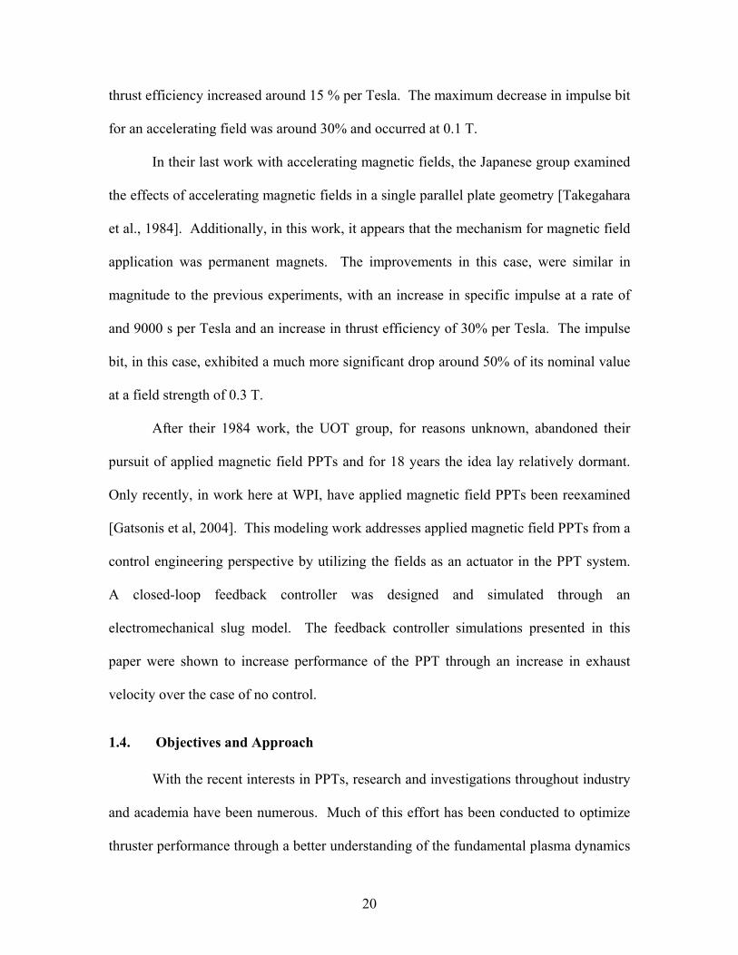
power level thrusters. Figures 2.7 and 2.8 display the plasma resistance versus plasma

temperature for the LES-6 and the LES-8/9 PPT for various electron number densities

using equation (2.25).

Figure 2.7 Plasma resistance model for LES-6 PPT.

Figure 2.8 Plasma resistance model for LES-8/9 PPT.

34

2.2.5. Summary of the Parallel-Plate Electromechanical Model

To wrap up this model derivation, the initial conditions of this system of two,

second order ODE’s must be specified. These are given as

( )0 0,sx = ( )0 0,sx = ( )0

0

0,t

I t dt=

=∫ ( )0 0.I = (2.26)

Taking the dynamic (2.17) and circuit (2.1) equations together with the initial conditions

(2.26) and substituting the mass distribution function (2.18) and the plasma resistance

model (2.25) constitute the generalized, one dimensional, parallel plate PPT model for

unsteady plasma acceleration,

( ) ( )( )00

1 t

c e pe pV I t dt I t R R R RC

− = + + + +∫

( ) ( ) ( ) ( )0 0 0 ,2c e s s

h h hL L x t I t x t I tw w w

δµ µ µ + + + + (2.27)

( ) ( ) 20

1 ,2s

d hmx t I tdt w

µ= (2.17)

( ) ( )1

1

0 1 1 ,st

x tm t m m

l

α−

= + − −

(2.18)

13 2

70

34

ln 1.24 10

8.08

e

e

p

e

Tn

hRT w

µ

τ

× = (2.25)

( )0 0,sx = ( )0 0,sx = ( )0

0

0,t

I t dt=

=∫ ( )0 0.I = (2.26)

This system can be solved for ( )sx t and ( )I t to and all other pertinent information, e.g.

velocity and voltage can be derived from this solution.

35

The energy equation for the circuit is of particular interest in this performance

optimization study. It can be derived from the circuit equation (2.27) by multiplying it by

( )I t and integrating over time,

( ) ( ) ( ) ( ) ( ) ( ) ( )2 2 2

0 0 0 0

1 1 .2 2

t t t t

c T T TdI t V dt I t L t dt R t I t dt I t L t dtdt = + + ∫ ∫ ∫ ∫ (2.28)

The term to the left equal sign may be evaluated by substituting for current,

( ) ( )cdV tI t C

dt= − (2.29)

This results in the energy equation for the PPT system.

( ) ( ) ( ) ( ) ( ) ( ) ( )2 2 2 220 0

0 0

1 1 1 1 .2 2 2 2

t t

c T T shCV C V t I t L t R I dt I x dtw

τ τ µ τ τ− = + + ∫ ∫ (2.30)

The first term on the left hand side represents the total energy stored in the capacitor at

0.t = The second term on the left hand side is the time varying energy stored in the

capacitor. The terms on the right are, respectively, the energy stored in the magnetic

field, the energy dissipated by Ohmic heating and the work done to accelerate the current

sheet mass.

a) Slug Operation

The generalized parallel plate PPT electromechanical model can be easily adapted

to the various operational modes of parallel plate PPTs. For example, in ablative PPTs

the propellant mass enters the current sheet very early in the acceleration process and is

accelerated electromagnetically together as one unit or “shot”. This model has been

come to be known as the one dimensional slug model of PPT operation. The GFPPT can

36

also be simulated by the slug model if the capacitor is discharged before the propellant

gas has been given enough time to expand away from the back of the GFPPT channel.

Mathematically, the generalized parallel plate PPT model can be easily

transformed into the slug model with a mass loading parameter 1α = . In this model, all

the propellant gas is assumed to be located all along the insulator face at 0t = . In the

limit that 1,α = there is no mass accumulation ( )( )0m t = as the current sheet travels

down the channel as a constant mass slug with , ( ) 0.m t m= Thus, the system of

equations with its accompanying initial conditions can be written as

( )00

1 t

V I t dtC

− =∫

( )( ) ( ) ( ) ( ) ( )0 0 0 ,2c e pe p c e s s

h h hI t R R R R L L x t I t x t I tw w w

δµ µ µ + + + + + + + + (2.27)

( ) ( ) 20 0

1 ,2s

hm x t I tw

µ= (2.31)

13 2

70

34

ln 1.24 10

8.08

e

e

p

e

Tn

hRT w

µ

τ

× = (2.25)

( )0 0,sx = ( )0 0,sx = ( )0

0

0,t

I t dt=

=∫ ( )0 0.I = (2.26)

Here, it can be seen that the only changes from the general one dimensional parallel plate

PPT model lie within Newton’s second law equation for the system (2.31).

37

b) Snowplow Operation

To model the majority of operational modes of GFPPTs, a variable current sheet

mass must be assumed. In the snowplow mode, the current sheet starts off with an

initially ionized mass or zero mass. This accelerating sheet sweeps up the mass it

encounters as it travels down the channel. Most snowplow models assume a constant

mass distribution throughout the channel ahead of the current sheet. This situation can be

modeled using a mass loading parameter equal to zero. Thus, the system of equations

with accompanying initial conditions becomes

( )00

1 t

V I t dtC

− =∫

( )( ) ( ) ( ) ( ) ( )0 0 0 ,2c e pe p c e s s

h h hI t R R R R L L x t I t x t I tw w w

δµ µ µ + + + + + + + + (2.27)

( ) ( ) ( ) ( ) 20

1 ,2s s

hm t x t m t x I tw

µ+ = (2.32)

( ) ( )1

1

0 1 1 ,st

x tm t m m

l

α−

= + − −

(2.18)

13 2

70

34

ln 1.24 10

8.08

e

e

p

e

Tn

hRT w

µ

τ

× = (2.25)

( )0 0,sx = ( )0 0,sx = ( )0

0

0,t

I t dt=

=∫ ( )0 0.I = (2.26)

If a non-uniform mass distribution is to be modeled, the general model (2.27), (2.32),

(2.18), (2.25) and (2.26) may be applied with a mass loading parameter between zero and

one. The kinetic gas theory mass model (2.21) described by Ziemer et al. [1998] can be

38

approximated using the mass distribution model (2.18) through the correct choice of

parameters α and .l

2.2. Generalized Electromechanical Model for a Coaxial PPT

Figure 2.9 Coaxial GFPPT.

Due to the operational similarity of coaxial PPTs with their parallel plate

counterparts, they can be modeled in the same way, as an electrical system interacting

with a mechanical system. As seen in comparing figure 2.10 with 2.3, the electrical

system is identical for both the coaxial and parallel plate one dimensional models with

the exception of the coaxial plate inductance term.

Figure 2.10 Circuit model of a coaxial PPT.

Accordingly, this general coaxial derivation is identical to the general parallel plate

derivation for equations (2.1) through (2.3) involving the circuit equation. Differences

39

arise due to the dissimilar induced magnetic fields and plasma current densities produced

by the devices.

2.2.1. Coaxial Self-Induced Magnetic Field

The induced magnetic field behind the current sheet within this coaxial conductor

can be found by applying Ampere’s Law to a surface S with radius r and an outer

contour C around the inner electrode (Figure 2.11) [Haus et al., 1989].

Figure 2.11 Coaxial PPT cutaway with uniform surface current.

The current in a coaxial conductor operated with a low characteristic pulse time will be

dominated by the skin effect. Accordingly, the current will flow nearly entirely on the

outer surface of the inner electrode and on the inner surface of the outer electrode. This

gives Ampere’s Law as

( ) ( )2 2

00 0

,i iB t rd K t rdπ π

φµ φ φ=∫ ∫ (2.33)

40

where Bφ is the self-induced azimuthal magnetic field and ( )iK t is the surface current

density on the inner electrode given by

( ) ( ) .2i

i

I tK t

rπ= (2.34)

Solving (2.33), substituting (2.34), and writing the azimuthal component as a vector field

gives

( ) ( )0 ˆ ,

2ind

I tt

rµ

π= − φB (2.35)

which fully describes the magnetic field in the region between the electrodes. The

current sheet current density will also have a different structure than for the parallel plate

geometry. Assuming the current is uniformly distributed throughout the sheet gives a

current density that varies in the radial direction between the electrodes as

( ) ( )ˆ.

2I t

trπδ

= − rj (2.36)

The magnetic field throughout the current sheet can be found by applying Ampere’s Law

in a similar way as was done for the parallel plate geometry. This gives the magnetic

field throughout the sheet as,

( ) ( ) ( )0 ˆ, , 1 .

2s

ind

I t x x tt x r

rµ

π δ −

= − −

φB (2.37)

The magnetic field in front of the current sheet can be found similarly and is equal zero

as it was for the parallel plate geometry. Taking (2.35) and (2.37) together with zero

field ahead of the current sheet gives the full description of the magnetic field used in this

general coaxial model

41

( )

( ) ( )

( ) ( ) ( ) ( )

( )

0

0

ˆ

ˆ

, 02

, , 1 , .2

0,

s

sind s s

s

I tx x t

rI t x x t

t x r x t x x tr

x x t

µπ

µ δπ δ

δ

− < <

−= − − < < +

> +

φ

φB (2.38)

2.2.2. Coaxial Electrode Inductance Model

Substituting (2.38) into equation (2.3) yields

( ) ( ) ( )PPT c et L I t L I tλ = + +

( )( ) ( ) ( )( )

( )2 2

0 00 0 0

1 ,2 2

s so o

i s i

x t x tr rs

r x t r

I t I t x x tr drdx r drdx

r r

δπ π

µ ϕ µ ϕπ π δ

+ −+ −

∫ ∫ ∫ ∫ ∫ ∫ (2.39)

which integrates to

( ) ( ) ( ) ( ) ( )0 0ln ln .2 4s o o

PPT c ei i

x t r rt L I t L I t I tr r

δλ µ µπ π

= + + +

(2.40)

This gives the coaxial electrode inductance model as

( )( ) ( )( )( )

( )0 0ln ln .

2 4ce s s o o

ce si i

x t x t r rL x tI t r r

λ δµ µπ π

= = +

(2.41)

Similar to the parallel-plate inductance model, for an infinitesimally thin current, 0,δ =

the model reduces to

( )( ) ( )( )( )

( )0 ln .

2ce s s o

ce si

x t x t rL x tI t r

λµ

π

= =

(2.42)

This coaxial inductance model is the same as found in Hart’s [1962] coaxial accelerator

model.

42

The motion of the coaxial current sheet described dynamically by Newton’s

second law (2.14). The Lorentz force for this geometry will be given by

( ) ( ) ( )2

00

ˆ1 ,2 2

s o

s i

x rs

Lx r

rI t I t x x t

drd dxr r

δ π

µ φπδ π δ

+ − = −

∫ ∫ ∫ xF (2.43)

which gives

( ) ( )

( )

( )

( )2

200

1ˆ ˆ1 ln .2 4

s o

s i

x t rs o

Lix t r

I t x x t rdx I tr r

δ µµπδ δ π

+ − = − =

∫ ∫F x x (2.44)

Substituting this into (2.15) gives the dynamic equation for the electromechanical model

( ) ( ) ( ) 20 ˆln .4

os

i

rd m t t I tdt r

µπ

=

x x (2.45)

2.2.3. Coaxial Plasma Resistance Model

The only other change to the general parallel plate model appears in the plasma

resistance model. With all other equations in this model remaining the same, the

resistance equation, in this coaxial geometry, will be written as

( )

,o ip

p o i

r rlRA r rσ σ δπ

−= =

+ (2.46)

where the area was taken at the average radius

( )2 .2

o io i

r rA r rδ π δπ+ = ⋅ = +

(2.47)

Substituting equations (2.22)-(2.24)into (2.46) yields the coaxial plasma resistance model

( )

13 2

70

34

ln 1.24 10

2.57 .

e

eo i

p

e o i

Tn

r rRT r r

µ

τ

× − =

+ (2.48)

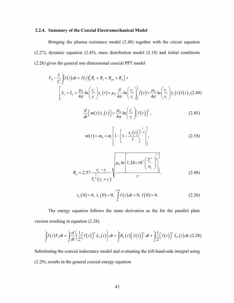
43

2.2.4. Summary of the Coaxial Electromechanical Model

Bringing the plasma resistance model (2.48) together with the circuit equation

(2.27), dynamic equation (2.45), mass distribution model (2.18) and initial conditions

(2.26) gives the general one dimensional coaxial PPT model

( ) ( ) 00

1 t

c e pe pV I t dt I t R R R RC

− = + + + +∫

( ) ( ) ( ) ( )0 00ln ln ln ,

4 4 4o o o

c e s si i i

r r rL L x t I t x t I tr r r

µ µδµπ π π

+ + + +

(2.49)

( ) ( ) ( ) 20 ln ,4

os

i

rd m t x t I tdt r

µπ

=

(2.45)

( ) ( )1

1

0 1 1 ,st

x tm t m m

l

α−

= + − −

(2.18)

( )

13 2

70

34

ln 1.24 10

2.57 .

e

eo i

p

e o i

Tn

r rRT r r

µ

τ

× − =

+ (2.48)

( )0 0,sx = ( )0 0,sx = ( )0

0

0,t

I t dt=

=∫ ( )0 0.I = (2.26)

The energy equation follows the same derivation as the for the parallel plate

version resulting in equation (2.28).

( ) ( ) ( ) ( ) ( ) ( ) ( )2 2 2

0 0 0 0

1 1 .2 2

t t t t

c T T TdI t V dt I t L t dt R t I t dt I t L t dtdt = + + ∫ ∫ ∫ ∫ (2.28)

Substituting the coaxial inductance model and evaluating the left-hand-side integral using

(2.29), results in the general coaxial energy equation

44

( ) ( ) ( )2 22 00 0

1 1 1 ln ln2 2 2 4 4

o oc c e s

i i

r rCV C V t I t L L x tr r

µ δµπ π

− = + + + +

( ) ( ) ( ) ( )2 20

0 0

ln .4

t to

T si

rR t I t dt I t x t dtr

µπ

+

∫ ∫ (2.50)

a) Slug Operation

The generalized coaxial PPT electromechanical model can be easily adapted to

the various operational modes of coaxial PPTs. A coaxial APPT can be modeled using a

“slug” mass model with a mass loading parameter 1.α = This slug model is also

applicable for a GFPPT operating with minimal propellant gas expansion. Thus, the

entire system of equations with its accompanying initial conditions can be written as

( ) ( ) ( )00

1 to i

c e pep o i

r rV I t dt I t R R RC r rσ δ

− − = + + + + + ∫

( ) ( ) ( ) ( )0 00ln ln ln ,

4 4 4o o o

c e s si i i

r r rL L x t I t x t I tr r r

µ µδµπ π π

+ + + +

(2.51)

( ) ( ) 200 ln ,

4o

si

rm x t I tr

µπ

=

(2.52)

( )

13 2

70

34

ln 1.24 10

2.57 .

e

eo i

p

e o i

Tn

r rRT r r

µ

τ

× − =

+ (2.48)

( )0 0,sx = ( )0 0,sx = ( )0

0

0,t

I t dt=

=∫ ( )0 0.I = (2.26)

45

b) Snowplow Operation

To model the majority of operational modes of coaxial GFPPTs, a current sheet

mass that is a function of sheet position was employed. As was done in the case of the

parallel plate snowplow model, this was done by using the mass distribution model with a

mass distribution parameter, 1.α < Using a mass distribution parameter equal to zero

simulates a uniform mass distribution throughout the channel. Thus, the entire system of

equations with its accompanying initial conditions is

( ) ( ) ( )00

1 to i

c e pep o i

r rV I t dt I t R R RC r rσ δ

− − = + + + + + ∫

( ) ( ) ( ) ( )0 00ln ln ln ,

4 4 4o o o

c e s si i i

r r rL L x t I t x t I tr r r

µ µδµπ π π

+ + + +

(2.53)

( ) ( ) ( ) ( ) ( ) 20 ln ,4

os s

i

rm t x t m t x t I tr

µπ

+ =

(2.54)

( ) ( )1

1

0 1 1 ,st

x tm t m m

l

α−

= + − −

(2.18)

( )

13 2

70

34

ln 1.24 10

2.57 .

e

eo i

p

e o i

Tn

r rRT r r

µ

τ

× − =

+ (2.48)

( )0 0,sx = ( )0 0,sx = ( )0

0

0,t

I t dt=

=∫ ( )0 0.I = (2.26)

2.3. Electromechanical Model for an Applied Field PPT

In order to simulate an applied magnetic field PPT the generalized

electromechanical PPT models must be modified. Specifically, external magnetic fields

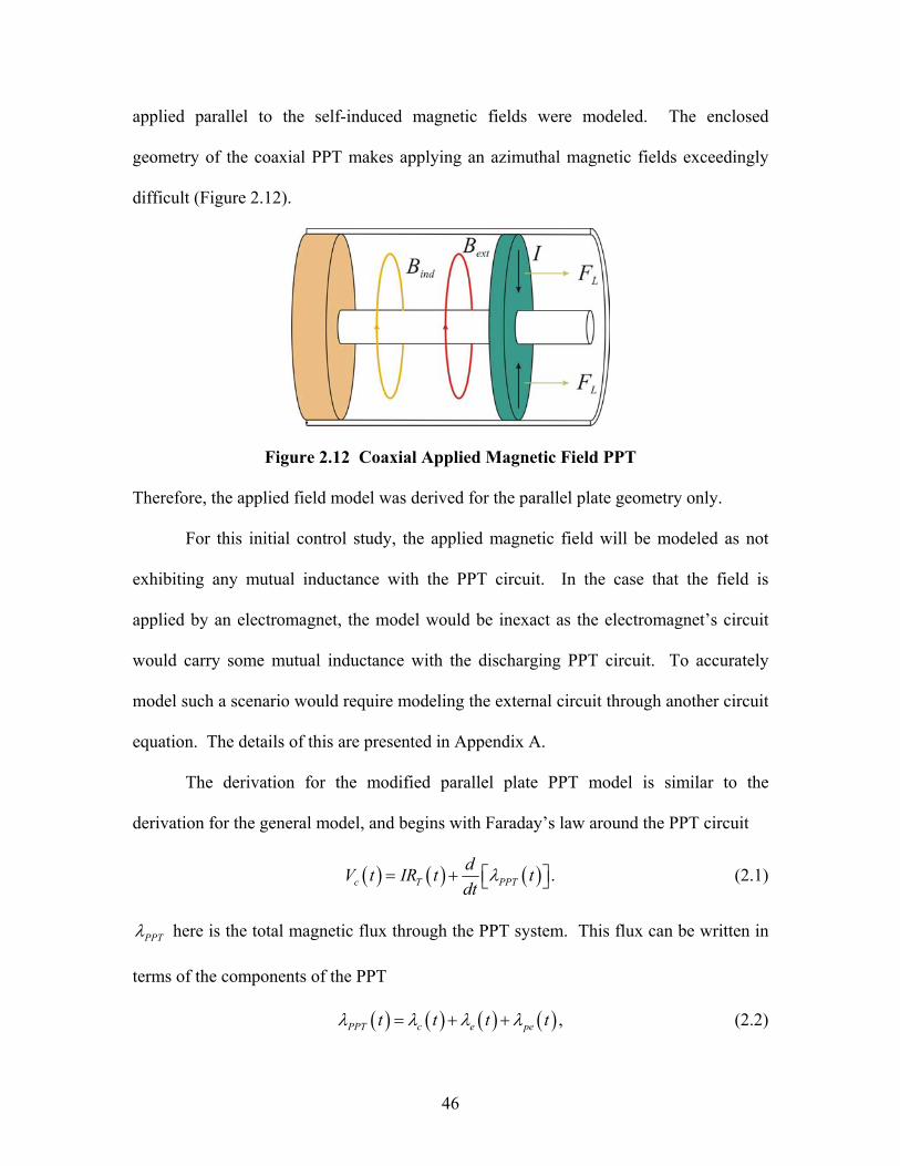
46

applied parallel to the self-induced magnetic fields were modeled. The enclosed

geometry of the coaxial PPT makes applying an azimuthal magnetic fields exceedingly

difficult (Figure 2.12).

Figure 2.12 Coaxial Applied Magnetic Field PPT

Therefore, the applied field model was derived for the parallel plate geometry only.

For this initial control study, the applied magnetic field will be modeled as not

exhibiting any mutual inductance with the PPT circuit. In the case that the field is

applied by an electromagnet, the model would be inexact as the electromagnet’s circuit

would carry some mutual inductance with the discharging PPT circuit. To accurately

model such a scenario would require modeling the external circuit through another circuit

equation. The details of this are presented in Appendix A.

The derivation for the modified parallel plate PPT model is similar to the

derivation for the general model, and begins with Faraday’s law around the PPT circuit

( ) ( ) ( ) .c T PPTdV t IR t tdt

λ = + (2.1)

PPTλ here is the total magnetic flux through the PPT system. This flux can be written in

terms of the components of the PPT

( ) ( ) ( ) ( ) ,PPT c e pet t t tλ λ λ λ= + + (2.2)

47

where the three terms on the right are, respectively, the magnetic flux due to the capacitor

inductance, the wire and lead inductance and the flux through the electrode channel.

Using the previous result for the self-induced magnetic field (2.9) and assuming the

external magnetic field is applied throughout the electrode channel and current sheet,

(2.2) may be written as

( ) ( ) ( ) ( ) ( )0 0 2PPT c e sh ht L I t L I t x t I tw w

δλ µ µ = + + + +

( ) ( )( )

( )( )

0 0 0

, , , , ,s s

s

x t x th h

ext extx t

B t x y dydx B t x y dydxδ+

+∫ ∫ ∫ ∫ (2.55)

where ( ), ,extB t x y is the magnitude of the external magnetic field. Assuming the applied

field has negligible spatial gradient over the electrode channel region yields

( ) ( ) ( ) ( ) ( ) ( ) ( )0 0 .2PPT c e s ext s

h ht L I t L I t x t I t hB t x tw w

δλ µ µ δ = + + + + + (2.56)

Substituting this into (2.1) gives the circuit equation for the modified system

( ) ( ) ( )( )00

1 t

c c e pe pV t V I d I t R R R RC

τ τ= − = + + + +∫

( ) ( ) ( ) ( ) ( ) ( ) 0 0 0 .2c e s s ext s

h h h dI t L L x t I t x t h B t x tw w w dt

δµ µ µ δ + + + + + + (2.57)

Notice that in comparing this equation with (2.27), the only modification is the addition

of the later term.

The dynamic equation derivation follows the general model with the only

deviation arising due to the difference in the magnetic field throughout the current sheet.

Taking the result from the parallel plate model and applying superposition gives the

magnetic field throughout the PPT

48

( )

( ) ( ) ( )

( ) ( ) ( ) ( ) ( )

( ) ( )

0

0

ˆ ˆ , 0

ˆ ˆ, 1 , .

ˆ ,

ext s

sext s s

ext s

I tB t x x t

wI t x x t

t x B t x t x x tw

B t x x t

µ

µ δδ

δ

+ < <

−= − + < < +

> +

y y

B y y

y

(2.58)

With a uniform current density throughout the current sheet

( ) ( ) ˆ,I t

twδ

= −j z (2.7)

the Lorentz force acting on the current sheet will be

( ) ( ) ( ) ( ) ( ) ( ) ( )( )

( )

0ˆ, 1s

s

x ts

s extcurrent x tsheet

I t h I t x x tt t t x dV B t dx

w

δ

µδ δ

+ − = × = − + =

∫∫∫ ∫F j B x

( ) ( ) ( )2

01 ˆ .2 ext s

h I t hI t B tw

µ + x (2.59)

Substituting this into Newton’s second law of motion yields

( ) ( ) ( ) ( ) ( )20

1 .2s ext

d hm t t I t hI t B tdt w

µ= + x (2.60)

Taking this dynamic equation with the circuit equation (2.57), the mass

distribution model (2.18), the resistance model (2.21)-(2.24) and initial conditions (2.26)

yields the parallel plate model modified to include an externally applied magnetic field.

( ) ( )( ) ( ) ( )0 0 00

12

t

c e pe p c e sh hV I d I t R R R R L L x t I t

C w wδτ τ µ µ − = + + + + + + + + ∫

( ) ( ) ( ) ( ) ( ) ( )0 ,s s ext s exth x t I t x t hB t x t hB tw

µ + + (2.57)

( ) ( ) ( ) ( ) ( )20

1 ,2s ext

d hm t t I t hI t B tdt w

µ= + x (2.60)

49

( ) ( )1

1

0 1 1 ,st

x tm t m m

l

α−

= + − −

(2.18)

13 2

70

34

ln 1.24 10

8.08

e

e

p

e

Tn

hRT w

µ

τ

× = (2.48)

( )0 0,sx = ( )0 0,sx = ( )0

0

0,t

I t dt=

=∫ ( )0 0.I = (2.26)

In the case of a constant external magnetic field, the final term of (2.57) will be zero.

This model was numerically integrated using the same method described in chapter 3 to

arrive at solutions for ( )I t and ( ).sx t

The energy equation for the circuit is again of interest with this modified model

and can be derived from the circuit equation following the procedure used for the general

model. Multiplying (2.57) by ( )I t and rearranging the terms gives the power equation

for the modified circuit,

( ) ( ) ( ) 2c TV t I t R I t= +

( ) ( ) ( ) ( ) ( ) ( ) ( )2 21 1 .2 2T T s ext

d dL t I t L t I t h x t B t I tdt dt + +

(2.61)

Substituting for the current in the capacitor power term on the right hand side

( ) ( )cdV tI t C

dt= − (2.29)

and integrating over time yields,

( ) ( )2 220

0

1 12 2

t

c TCV C V t R I dτ τ− = + ∫

50

( ) ( ) ( ) ( ) ( ) ( ) ( )2 2

0 0

1 1 .2 2

t t

T T s extdL t I t L I d h I x B ddt

τ τ τ τ τ τ τ+ + ∫ ∫ (2.62)

This modified energy equation is the same as the original equation apart from the last

term. This term accounts for the work performed by the circuit on the current sheet mass

due to the external magnetic field and the energy stored in the circuit magnetic field due

to the changing flux of the external magnetic field.

( ) ( ) ( ) ( ) ( ) ( ) ( ) ( ) ( )0 0 0

t t t

s ext s ext s extdh I x B d h x B I d h x B I ddt

τ τ τ τ τ τ τ τ τ τ τ τ= + ∫ ∫ ∫ (2.63)

51

3. Numerical Implementation, Software Implementation and Model Validation

Chapter 3

Numerical Implementation, Software

Implementation and Model Validation This chapter discusses several practical issues pertaining to the one dimensional

PPT models. Here, the numerical method employed in solving the model equations is

presented. Furthermore, the GUI software environment developed to change model

parameters and view the solution results is described. Finally, the model is validated for

the case of ablative PPTs by comparison with the LES-6 and LES-8/9 PPTs.

3.1. Numerical Implementation

The second order systems of coupled nonlinear integro-differential equations

were solved numerically for both coaxial [Equations (2.49), (2.45), (2.18), (2.48) and

(2.26)] and parallel plate geometries [Equations (2.27), (2.31), (2.18), (2.25) and (2.26)]

and slug and snowplow operating conditions. To accomplish this, each set of equations

were written as a system of four first-order differential equations through the following

state space variables

( ) ( )1 ,sx t x t= (2.64)

( ) ( )20

,t

x t I dτ τ= ∫ (2.65)

( ) ( )3 ,sx t x t= (2.66)

52

( ) ( )4 .x t I t= (2.67)

In this state space form the parallel plate slug model equations become

( ) ( )1 3 ,x t x t= (2.68)

( ) ( )2 4 ,x t x t= (2.69)

( ) ( )'

23 4

0

1 ,2

peLx t x t

m = (2.70)

( ) ( ) ( ) ( )

( )2 4 4 0

4

1

,T T

T

x t L t x t R x t VCx

L t

− − − + = (2.71)

( ) ( ) ( ) ( )1 2 3 40 0, 0 0, 0 0, 0 0,x x x x= = = = (2.72)

where ,T c e pe pR R R R R= + + + ( ) ( )T c e peL t L L L t= + + and pR is given by (2.48) and

( )peL t is given by (2.13).

The above nonlinear ordinary differential equation (ODE) system was integrated

numerically by implementing MATLAB’s® nonlinear ODE solvers. For initial

numerical solutions, LES 6 PPT parameters were used (Table 1). It was initially thought

that there would be possible issues with ODE stiffness and as such, the initial solvers

implemented were ode23s and ode15s. The validity and accuracy of these methods was

checked by verifying that system energy was conserved for both the general model and

the modified model. Since the circuit equation is a statement of energy conservation for

the electrical system this is a valid requirement for an acceptable method. Using the

terms in (2.30) the energy on the capacitor is given by

( ) ( ) 21 ,2c cE t C V t = (2.73)

53

where ( )cV t is the voltage on the capacitor. The voltage on the capacitor was calculated

at each timestep using

( ) ( ) ( )0 0 20

1 1 .t

cV t V I t dt V x tC C

= − = −∫ (2.74)

The energy dissipated by ohmic heating is given by

( ) ( ) ( ) ( ) ( )2 24

0 0

.t t

T TE t R I d R x t dτ τ τ τ τΩ = = ∫ ∫ (2.75)

The integral appearing in this equation was solved numerically using a trapezoidal sum.

The energy stored in the magnetic field is given by

( ) ( ) ( ) ( ) ( )2 20 0 1 4

1 1 .2 2B c e s c e

h hE t L L x t I t L L x t x tw w

µ µ = + + = + + (2.76)

Finally, the energy given to the accelerated current sheet is given by

( ) ( ) ( )2 20 0 3

1 1 .2 2KEE t m V t m x t = = (2.77)

The modified model has an extra term in its energy equation (2.62) in comparison with

the general model energy equation. This term accounts for the work performed by the

circuit on the current sheet mass due to the external magnetic field and the energy stored

in the circuit magnetic field due to the changing flux of the external magnetic field.

( ) ( ) ( ) ( ) ( ) ( ) ( ) ( ) ( )3 4 1 40 0 0

t t t

s ext ext extdh I x B d h x x B d h x x B ddt

τ τ τ τ τ τ τ τ τ τ τ τ= + ∫ ∫ ∫ (2.78)

Summing these components at each timestep yields the total energy throughout the

discharge. By choosing a sufficiently tight tolerance setting both stiff ODE solver

methods yielded solutions that conserved the system energy (Figure 4.1 and Figure 4.2).

54

Figure 3.1 General model simulation output using LES-6 thruster parameters.

Figure 3.2 Nominal applied magnetic field PPT simulation (Bext =0.3 T).

In addition to the stiff solver, the non-stiff solvers; ode23, ode45 and ode113,

were implemented in numerically integrating the systems. If the system has stiffness

55

issues, these solvers would be very inefficient arriving at a solution, requiring a

significant number of timesteps and run time to solve. However, these solvers were

generally found to integrate the system with fewer timesteps than the stiff solvers, leading

to the conclusion that the system is not particularly stiff. The solver chosen for use

throughout the thesis was the one that conserved system energy while minimizing the

tolerance, timesteps, and computer run time. This was determined to be ode45 at

absolute and relative tolerance levels of 1e-6. Ode45 is a single step method based on an

fourth and fifth order explicit Runge-Kutta formula called the Dormand-Prince pair

[Dormand et al., 1980].

Two solver schemes were implemented in solving the system. The MATLAB®

ODE solvers were applied in an automatic way by allowing them to determine the length

of each timestep. Depending on the input tolerance level, the solver automatically

determines the length of each timestep based upon the dynamics of the ODE at that

timestep. This results in a solution with the fewest number of calculations and timesteps

while maintaining the accuracy determined by the tolerance level. However, as a way to

implement more control over the solution, another method, utilized in the work by

Demetriou et al. [2003], was also implemented. This method requires user inputs for the

number of timesteps, tolerance and number of integration points in each timestep. The

method divides up the time interval into subintervals each the length of the timestep. A

MATLAB® ODE solver is applied over this interval using the solution from the last

timestep for its initial values. The solution is calculated over the timestep subinterval at a

number of points equal to the user input number of integration points. The final output is

taken as the solution at the endpoints of each subinterval. In addition to giving the user

56

more control in choosing the timestep length, this method will also generally give a more

accurate integration. The major drawback with this method is the computational run

time, taking up to minutes to arrive at a solution versus seconds with the automatic

solution method.

In addition to the energy being calculated, various other thruster performance

parameters were determined or calculated. The exhaust velocity was taken to be the

velocity at which the position of the current sheet was equal to the length of the thruster.

This system state is defined as

( )* ,e sx x t= (2.79)

where

( )* *: .t x t l= (2.80)

The specific impulse was calculated from the exhaust velocity as

,esp

xIg

= (2.81)

where g is the acceleration of gravity at sea level. To calculate the impulse bit, the

impulse acting on the current sheet was calculated as a function of time through

( ) ( ) 20

0

1 .2

t

bithI t I t dw

µ τ = ∫ (2.82)

This integral was solved numerically using the trapezoidal summation and the impulse bit

for the simulation was taken to be the impulse at the current sheet exit time.

3.2. Software Implementation

The general PPT model has the potential for 21 input parameters. With such a

significant number of model inputs, it was decided that a graphical user interface (GUI)

57

application should be developed to provide an easy means for changing model inputs and

visualizing simulation results. To accomplish this, MATLAB’s® Graphical User

Interface Development Environment (GUIDE) was utilized. GUIDE provides all the

necessary tools to design and write the code for a MATLAB® GUI. This allowed all of

the model inputs and resulting plots to be displayed in the same window. Figure 4.3

displays the PPT model GUI.

Figure 3.3 MATLAB® one dimensional PPT model GUI.

In the first user inputs section, the “Thruster Specifications” as user can change

the geometry settings, the circuit parameters, and plasma resistance model parameters.

Additionally, a user can turn the plasma resistance model off using a user input value of

resistance. In the second section, “Model Specifications” a user defines what type of

58

model will be simulated; slug, snowplow (constant density distribution) and snowplow

(variable density distribution). Additionally, here a user can simulate certain thrusters,

whose model parameter sets have been previously entered. The last user input section,

“Solver Specifications” allows a user control over how the system is solved. The user

can choose from the ‘automatic’ MATLAB® solver and the ‘manual’ solver. The

automatic solver only has options for changing the tolerance. Using the manual solver a

user can change the tolerance, number of timesteps and the number of integration points

throughout each timestep. Lastly, here a user specifies the total time domain the system

is solved over.

3.3. General Model Validation

The general model was validated for the case of a parallel plate ablative PPT

(Table 4.1).

Table 3.1 General Model Validation

Parallel Plate Coaxial

Slug Snowplow Slug Snowplow Ablative yes no no no Gas-Fed - - no no

In order to validate the general model, simulation results were compared with data (Table

4.2) from two parallel plate thrusters; the LES 6 [Vondra et al., 1970 and 1971] and the

LES 8/9 [Vondra et al., 1973], [Leiweke, 1996].

Table 3.2 Experimental Parallel Plate PPT Data

Thruster LES-6 PPT LES-8/9 PPT

Initial Voltage (V) 1360 1538 Capacitance (µF) 2 17

Capacitor Resistance (mΩ) 30 30 Initial Inductance (nH) 34 35

Gap Width (cm) 3 2.54

59

Plate Width (cm) 1 2.54 Channel Length (cm) 0.6 2.54

Mass Bit (µg) 10 28.5 Pulse Time (µs) 0.4 1.0

Plasma Temperature (eV) 1.5 5 Electron Density (m-3) 1e21 1e21

It should be noted that the value of capacitor and wire and lead resistance for the LES 8/9

was determined from the measured total resistance of 45 mΩ and a plasma resistance on

the order of 15 mΩ [Leiweke, 1996]. The average plasma temperature for the LES 8/9

was estimated based on langmuir probe plume measurements [Gatsonis et al., 2001].

Using this data as inputs into our model, simulation results were compared with

experimental data. The current and voltage waveforms for the LES-6 PPT were found in

Waltz [1969]. In this work, a voltage measurement was taken as closely as possible to

the capacitor terminals. Because the capacitor inherently has some internal resistance

and inductance, this measurement does not correspond to an actual capacitor voltage

measurement (Figure 4.4).

Figure 3.4 LES-6 circuit with voltage measurement.

However, from this data the actual circuit current was found by solving the following

second-order ODE

( ) ( ) ( ) ( ).m c cCV t I t R CI t L CI t= − − − (2.83)

60

This experimental data was then plotted along with the simulation data for comparison

(Figure 4.5).

Figure 3.5 LES-6 experiment and simulation comparison.

The vertical dotted line indicates the time at which the current sheet exits the thruster for

the simulation. The disagreement between the experiment and simulation can be mainly

attributed to the constant plasma resistance in the model. This value was calculated by

the plasma resistance model to be 0.074 Ω. In the real thruster, the plasma resistance will

vary as the plasma is being formed and as the electron temperature and number density

change. This modeling issue shows itself the most at the beginning of the discharge

while the plasma is being formed and is evident in the initial “hitch” in the derived

current waveform. According to Waltz [1969] the plasma resistance at this time achieves

a maximum of 0.3 Ω. Despite this, the overall dynamics of the PPT LCR circuit appear

to be well matched. Table 4.3 compares the exit velocity, specific impulse and impulse

bit of the actual thruster and this simulation [Vondra et al., 1970]

61

Table 3.3 LES-6 simulation validation.

Experimental Simulation

Exit Velocity (ms-1) 3000 2975 Specific Impulse (s) 312 303 Impulse Bit (µN-m) 32 30

The slight underprediction in performance values is likely due a combination of a

variable plasma resistance and the presence of gas dynamic effects in the real thruster.

For the LES 8/9, the experimental voltage waveform data was found published in

Leiweke [1996]. Like the LES-6, this voltage measurement did not correspond exactly

with the capacitor voltage due to the internal capacitor resistance and inductance. This

experimental waveform was plotted along with the simulation data for comparison

(Figure 4.6). Though no current waveform could be located throughout literature, the

experimental peak current of 19 kA was found published in Vondra et al. [1973].

Figure 3.6 LES-8/9 experiment and simulation comparison.

62

The vertical dotted line again indicates the time at which the current sheet exits the

thruster for the simulation. Like for the LES-6, the overall dynamics of the LCR circuit

appear to be fairly well matched. Though there is an under prediction in the voltage

reversal, the maximum simulation current of 20 kA compares very well with the actual

thruster (19 kA). The plasma resistance model gives a value of 0.011 Ω. Table 4.4

compares the exit velocity, specific impulse and impulse bit of the actual LES-8/9 and the

simulation [Vondra et al., 1973].

Table 3.4 LES-8/9 simulation validation.

Experimental Simulation

Exit Velocity (ms-1) 9810 9674 Specific Impulse (s) 1000 986 Impulse Bit (µN-m) 300 276

The comparison here is very similar to the LES-6. Again, the slight underprediction by

the model may be attributed to a variable plasma resistance and the presence of gas

dynamic effects in the real thruster. Looking at the results of both simulations, it can be

concluded that the one-dimensional model predicts parallel plate PPT performance very

well

3.4. Modified Model Validation

The modified model was validated for the case of a constant magnetic field

applied by permanent magnets. Modified model simulation results were compared with

data from the 1984 UOT parallel plate thruster. This data set was chosen due to its

relative completeness and also because permanent magnets were utilized in applying the

external magnetic field. This was the simplest case to validate and therefore provided a

solid baseline comparison. For model inputs, the data presented in Table 2.1 was

utilized. This data set was complete excepting resistance data. The plasma resistance

63

model was unable to be utilized due to a lack of plasma temperature and electron density

data for a high energy (125 J) PPT. Therefore, to complete the data set, the capacitor

resistance and plasma resistance were set to 0.03 Ω and 0.015 Ω, respectively, for all the

simulations. These values correspond closely to the values found in the LES-6 and LES-

8/9 thrusters. For each simulation, the external magnetic field was applied over the first

1.75 cm of the electrode length. This was in agreement with the experimental setup

described in the paper [Takegahara et al., 1984]. The mass distribution was modeled in

each simulation as a slug distribution with all the mass contained within the current sheet

at 0.t =

Figures 4.6 and 4.7 compare the simulation and experiment results [Takegahara et al.,

1984] for specific impulse, thrust efficiency and impulse bit.

Figure 3.7 Specific impulse and thrust efficiency validation comparison.

Figure 3.8 Impulse bit validation comparison.

64

While the simulation results show good overall agreement with the experimental

values, there did appear to be a general divergence between the two. As can be seen in

the figures, the simulation tends to over-predict the PPT performance with no applied

magnetic field, under-predict at the highest field value and give generally very good

agreement at the intermediate value. This deviation is most certainly due to the model

not accounting for gas dynamic effects. As discussed in Chapter 1, an accelerating

applied magnetic field has the effect of causing a parallel plate PPT to operate

electromagnetically versus gas dynamically. In these validation simulations the entire

measured mass bit was assumed accelerated electromagnetically. In reality, only a

fraction of the mass would be ionized and accelerated electromagnetically. The

remaining fraction of mass, would gas dynamically expand away from the thruster as a

cloud of neutrals. This phenomenon was particularly prevalent in the thruster utilized for

this validation. This is evidenced by the large decrease in mass bit (300 to 60 µg) with

accompanying increase in applied field strength. This conclusion would lead one to

wonder why the simulation was not more accurate at the higher value of applied magnetic

field. The likely answer to this is an under-estimation of the circuit resistance (capacitor

and plasma). Using a lower value of resistance in the simulation would have the effect of

shifting all the results up. This would cause a better matching of simulation and

experiment at the higher value of applied magnetic field and an increasing divergence

with decreasing applied field strength. However, despite this digression, the modified

model appears to, quite satisfactorily; predict the performance of a parallel plate PPT

under the influence of a constant magnetic field applied by permanent magnets.

65

4. Control Strategy and Analysis

Chapter 4

Control Strategy and Analysis

The overall objective of this work is the development of a control scheme to

optimize PPT performance. In this study, an open-loop flow controller was investigated,

developed and applied. An open-loop flow control system consists of a dynamic flow

model, a control objective, a flow actuator and an open-loop controller (Figure 5.1). The

actuator is some type of model input that can be utilized to control or manipulate the

model outputs.

Figure 4.1 Closed-loop and open-loop flow control.

A closed-loop or feedback flow control system consists of a dynamic flow model, a

control objective, flow actuator, flow sensor (model outputs) and a controller which

commands the flow actuator in response to flow sensor outputs.

4.1. Control Objective and System

There are a number of PPT performance parameters that could be optimized.

These include, but are not limited to, specific impulse, impulse bit, thrust efficiency and

66

thrust-to-power. The specific impulse and thrust efficiency were chosen for optimization

based on the current trends in PPT use on small satellites. On these satellites, an

advantage PPTs inherently have is in their small impulse bits. As such, increasing the

impulse bit will not be specifically addressed in this thesis. A high specific impulse on

the other hand is desirable as it reduces the propellant mass needed to satisfy the mission

∆V requirements.

The thrust efficiency of these devices is significantly lower than other electric

propulsion devices and offers considerable opportunity for improved performance.

Previous flight qualified PPTs have produced thrust efficiencies between 0.06 and 0.13

[Myers et al., 1994]. However, Burton et al. [1998] estimated that rectangular and

coaxial PPTs have a maximum possible efficiency of 0.44 and 0.60, respectively. The

thrust efficiency is given as the ratio of directed exhaust kinetic energy to energy initially

stored on capacitor

( )

22

220 0

0

12 .12

e ee e e

t

m xKE m xE CVCV

η = = = (3.1)

The specific impulse can also be written in terms of the mass-averaged exhaust velocity

as

.esp

xIg

= (2.81)

This shows that the specific impulse and thrust efficiency will be maximized by

maximizing the thruster exhaust velocity. Accordingly, the control objective is an

increase or maximization of thruster exhaust velocity over nominal operating conditions.

67

The flow actuator is the element of the control system that affects the model or

device in such a way as to manipulate it to produce some desired output. An externally

applied magnetic field was chosen to accomplish this task. It has recently been suggested

in literature that externally applied magnetic fields will increase PPT performance

[Burton et al., 1998], [Ziemer et al., 1999]. Furthermore, a group at the University of

Tokyo successfully utilized both permanent magnets and electromagnets to apply

external magnetic fields to parallel plate and coaxial laboratory PPTs [Kimura et al., 1978

and 1979]. Their experiments with the parallel plate PPTs show an increase in specific

impulse and thrust efficiency with the application of self-field augmenting external

magnetic fields [Takegahara et al., 1984]. Lastly, an external magnetic field can be

introduced to the general one-dimensional PPT model with relative ease through the

circuit equation. One drawback of external magnetic fields is the difficulty in

implementing them on coaxial PPTs. While parallel plate PPTs can be augmented with

magnetic fields quite readily, coaxial geometries are much less conducive to externally

applied magnetic fields (Figure 2.10). Because of this, the remainder of this thesis will

focus on the parallel plate geometry. In parallel plate PPTs, Lorentz force accelerating or

retarding fields may be applied with permanent magnets (Figure 5.2) or electromagnets

68

Figure 4.2 Parallel plate PPT with external magnetic field applied via permanent

magnets.

The controller is central to the control system, as it carries out the control strategy

by operating the flow actuators. Three configurations of control were identified for the

possibilities of simulation; open-loop constant input, open-loop variable input, and close-

loop control. In open-loop control, the command signal sent to the actuator by the

controller can be either a constant value or a function of time. In closed-loop control, the

command signal is a function of the sensor outputs. In this initial control study, an open-

loop controller having constant applied magnetic field strength was examined. Despite

this, all three will be briefly described here. Open-loop constant input control represents

the simplest case that could be applied. In this case, a constant magnitude magnetic field

is applied over a length of the PPT channel. This field may be applied either with

permanent magnets or electromagnets. An electromagnet may be utilized in this case by

the coupling of an external LCR circuit with the PPT circuit as seen in Figure 5.3.

69

Figure 4.3 Open-loop controller using coupled external LCR circuit.

The external LCR circuit must have a discharge time much greater than the PPT circuit

discharge time for the applied magnetic field to be quasi-static throughout the discharge.

A time-variable open-loop controller could be implemented by applying an external

magnetic field which varies over the length of the thruster channel through the use of a

permanent magnet. Alternatively, this controller could also be implemented by utilizing

an LCR circuit with a discharge time on the same order as the PPT discharge time. A

closed-loop controller could be applied through the use of a similar coupled external

circuit except, in this case, the capacitor would be replaced with a controllable voltage or

current source (Figure 5.4). The models, which arise in the case of external circuits, are

presented in Appendix A.

70

Figure 4.4 Closed-loop controller using coupled external circuit with voltage source.

4.2. Control Analysis

With the above model validated for the case of a constant applied magnetic field,

it is of interest from a controls engineering standpoint to analyze the resulting nonlinear

dynamic system. Using the previously defined state-space variables (2.64)-(2.67), and

assuming the plasma resistance is constant, the above modified model can be written in

state space as

1 3,x x= (3.2)

2 4 ,x x= (3.3)

23 0 4 3 4

1 ,2 ext

h m hx x x x Bmw m m

µ= − + (3.4)

( )

0 2 0 3 4 4 3 1

41

1

,T ext ext

T

hV x x x R x x hB x hBC wx

L x

µ − − − − − = (3.5)

where T c e pe pR R R R R= + + + and ( )1 0 1.T c ehL x L L xw

µ= + +

71

Defining the state vector field, the input vector field and the drift vector field,

respectively,

( )

( )( )( )( )

1

2

3

4

,st

x tx t

tx tx t

=

x (3.6)

( )( ) ( )

( )( )

41

3

0 1

00

,

c e

h x tt mx t h

hL L x tw

µ

− = − + +

g x (3.7)

( )( )( )

( )

2

1

0 1

000 ,

c e

tx t h

hL L x tw

µ

= −

+ +

g x (3.8)

( )( )

( )( )

( ) ( )

( ) ( ) ( ) ( ) ( )

( )

3

4

20 4 3

0 2 0 3 4 4

0 1

12 ,

1T

c e

x tx t

h mx t x tmw mt

hV x t x t x t R t x tC w

hL L x tw

µ

µ

µ

− = − − − + +

f x (3.9)

( ) ( )extu t B t= (3.10)

the above state space can be written as

( ) ( )( ) ( )( ) ( ) ( )( ) ( )1 2 ,t t t u t t u t= + +x f x g x g x (3.11)

72

Since only the case of a constant magnetic field has been validated and in order to help

simplify this analysis, the time derivative term appearing in the numerator in (3.5), will

be dropped resulting in the following state space system

( ) ( )( ) ( )( )1 .t t t u= +x f x g x (3.12)

In evaluating the equilibrium points in the drift vector field, ( )( ) ,tf x it can be

easily seen that this system is in equilibrium at the following points

( )

( )1

0 .00

e

x tV C

t

=

x (3.13)

Physically, this equilibrium line represents the location in the manifold spanned by the

state vector with the minimum total system energy. Since the location of the current

sheet, ( )1 ,x t does not affect the system energy, it can be located anywhere. The next

value in the vector, 0 ,V C corresponds with the point at which all charge initially on the

capacitor has left. The last two values correspond to states of no kinetic energy or circuit

energy. Based on this physical interpretation and with the knowledge the system satisfies

energy conservation through the circuit equation, this equilibrium point should be stable.

4.2.1. Reachability

The notion of reachability addresses the capability of a system’s input actuators to

bring the system to a different state. In other words, given the correct choice of input,

what can be said about the set of points that can be reached from the initial state in a

finite time [Nijmeijer et al., 1990]. For the goals of this study, in increasing the exhaust

velocity state, this question is critical. For nonlinear systems, several statements of

73

reachability exist, however, all of them are of local nature due to their inclusion of a

linearization of the system. This is due to the fact that, for a nonlinear system, a ‘large’

distance or a ‘long’ time may be required in order to reach points near some initial state

[Casti, 1985]. In addition to this local description, nonlinear systems also have

reachability specified as either strong or weak. The concept of strong reachability

contrasts with weak reachability in that, it provides for a symmetric statement of

reachability. That is, in weak reachability, some state may be reachable from some initial

state, but the converse would not be true, while in strong reachability, the states are both

reachable from each other. The reachability test conducted in this study, which provides

a statement of the system’s locally strong reachability, is found in Nijmeijer et al. [1990].

Like all statements of controllability and reachability, a relatively simple, albeit lengthy,

algebraic test, leads to a statement of a nonlinear system’s locally strong reachability.

This test involves the calculation of the determinant of the systems strong accessibility

algebra. If the determinant is nonzero, the input vectors contained within the strong

accessibility algebra are linearly independent, span n and the system is locally strongly

accessible.

( )0det 0C ≠ (3.14)

The strong accessibility algebra is given by

[ ]0 1 2 3 4, , , ,C = g g g g (3.15)

where

2 1 1[ ,[ , ] ] ,LB LB=g g f g 3 2 1[ ,[ , ] ] ,LB LB=g g f g 4 3 1[ ,[ , ] ] .LB LB=g g f g (3.16)

74

The brackets in (3.16) represent Lie bracket operations. These Lie bracket calculations

were found to be quite tedious for the PPT system, therefore MAPLE® was utilized to

perform them.

The result of this reachability test was that the system was found to be locally

strongly accessible as long as the velocity ( )3x t and the current ( )4x t are not both

equal to zero. This would physically make sense, as the external field would require

some current or some sheet movement in order to influence the system.

75

Chapter 5

Controller Simulations 5. Controller Simulations

The constant open-loop controller was simulated by the modified model for the

cases of the 1984 UOT PPT, the LES-6 and the LES-8/9. These thrusters represent a

broad range of PPT capacitor energy levels (1.8, 20 and 125 J) and parallel plate

geometries. Since each of these thrusters is ablative, the slug mass distribution model

was utilized. In the case of 1984 UOT PPT the experimental mass bit data was utilized in

the simulations. However, in the case of the LES-6 and LES 8/9 a constant value of mass

bit was simulated. Though this is in contrast with previous UOT experimental data,

which indicated an initial drop in mass bit with increasing field strength, for the purposes

of these simulations it is a sufficient approximation. It should also be noted that the UOT

PPTs all had propellant arrangements along the direction of the current sheet propagation.

This would result in thrusters that operate predominately gas-dynamically, with large

measured mass bits that would be reduced significantly with accelerating external

magnetic fields. These large mass bits are indeed represented experimentally in the UOT

measurements. For example, for a 14.5 J UOT PPT operating with no applied magnetic

field, the mass bit was measured to be over 60 µg, compared to 28.5 µg for and LES-8/9

operating at a higher 20 J [Kimura et al., 1979]. The LES-8/9 and LES-6, with their

propellant at the back of the channel, therefore, should be more ‘immune’ to mass bit

decreases with accelerating fields.

76

The external field was applied up until the end of the thruster channel or at the

point where the current reversal began. This later restriction results in order to apply only

an accelerating external field. With a constant direction and magnitude external field,

were the current to reverse with the current sheet still moving through the field, a

decelerating Lorentz force would result. Accordingly, for each thruster, it is assumed this

approach will maximize the effect of the controller on the exhaust velocity. For each

value of magnetic field strength, an initial simulation was run with the external field

applied over the entire length of the thruster channel to check for the presence of current

reversal. If the current did not reverse before the sheet exhausted, this simulation would

stand. However, if the current was found to reverse in the channel, the position this

reversal initiated was determined. A final simulation was then run, with the external field

applied up until this point. In the case of the LES-6 and LES-8/9 the mass bit utilized in

each simulation

5.1. 1984 UOT PPT

In the 1984 UOT PPT validation simulation presented in section 3.4, the external

field was applied only over the first 1.75 cm of the thruster channel. As can be seen in

Figure 6.1, while this will include the current peak, there is a portion of the discharge

with very high current for which an accelerating applied magnetic field is not being

applied. The points in the figure represent exhaust values, while the line represents the

time at which the current sheet is no longer influenced by the external magnetic field.

77

Figure 5.1 1984 UOT PPT simulation current and distance (Bext = 0.3).

In the present set of simulations, the external field was applied over the entire

length of the thruster channel. Through this, a comparison was made between applying a

magnetic field over a portion of the discharge versus the entire discharge. It should be

noted that the field was applied over the entire channel length as the simulation indicated

no current reversal for all cases. Figures 6.2 and 6.3 plot the comparison for specific

impulse, thrust efficiency and impulse bit over applied magnetic field strength. All plots

compare only simulation results.

Figure 5.2 Specific impulse and thrust efficiency comparison.

78

Figure 5.3 Impulse bit comparison.

As can be seen in these comparisons, the performance benefits increase with applied field

strength. At a field strength of 0.3 T, these improvements are on the order of 10% for

specific impulse and thrust efficiency, with the impulse bit showing only a slight

increase. Whether these performance improvements are worthwhile would depend upon

the modification needed to apply them. That, of course, would have to be answered in an

analysis of the hardware needed to apply these fields, which is beyond the scope of this

study.

5.2. LES-6

The LES-6 was simulated with accelerating applied field strengths of 0, 0.25, 0.5,

0.75 and 1.0 T. The mass bit utilized in these simulation was the experimentally

measured value of 10 µg. Since, the current was found to reverse before current sheet

exhaust, the external magnetic field was applied up until the point that current reversal

was initiated. The following plots (Figure 6.4) display the effect of the fields on the

current sheet position and velocity.

79

Figure 5.4 Effects of constant magnitude externally applied magnetic fields on

current sheet position and velocity for the LES-6.

As can be seen in Figure 6.4, by increasing the field strength, the exhaust velocity of the

thruster can be increased. However, this effect appears to diminish with increasing field

strength. The current and voltage waveforms are significantly modified by the emf

generated by the applied magnetic field. The following plots (Figure 6.5) show this

effect.

80

Figure 5.5 Effects of constant magnitude externally applied magnetic fields on

current and capacitor voltage for the LES-6.

As can be seen in the current waveforms, for all magnitudes of applied field, current

reversal occurs. For 0.75 and 1.0 T, however, this reversal is small and near the exit of

the thruster. Both the current and voltage waveforms exhibit a trend of decreasing

amplitude with increasing applied magnetic field strength. This effect on current was

observed in the UOT experiments [Kimura et al., 1979] and is most likely due to the emf

generated by the applied field in the PPT circuit. Figure 6.6 shows the performance

enhancements of externally applied magnetic fields.

Figure 5.6 Effects of accelerating magnetic fields on LES-6 performance.

81

These plots show significant performance enhancements with increasing

externally applied accelerating magnetic fields. Each performance term increases

approximately linearly as field strength, with the specific impulse increasing 740 s per

Tesla, the thrust efficiency increasing 28 % per Tesla and the impulse bit increasing 72

µN-s per Tesla.

5.3. LES-8/9

Like the LES-6, the LES-8/9 was also simulated with accelerating applied field

strengths of 0, 0.25, 0.5, 0.75 and 1.0 T. As will be seen in figure 5.8, the simulation

predicted no current reversal for all applied field strengths and so the field was applied

over the entire length of the channel. The plots in Figure 6.7 display the effects of the

fields on the current sheet position and velocity.

82

Figure 5.7 Effects of constant magnitude externally applied magnetic fields on

current sheet position and velocity for the LES-8/9.

The effects here are virtually the same as for the LES-6. The current and voltage

waveforms displayed in Figure 6.8 show the same characteristics as the LES-6, with

diminished peak amplitude.

Figure 5.8 Effects of constant magnitude externally applied magnetic fields on

current and capacitor voltage for the LES-8/9.

83

As can be seen in these current waveforms, there was no current reversal for any of the

cases with applied magnetic fields. Figure 6.9 displays the performance enhancements of

externally applied magnetic fields in this thruster.

Figure 5.9 Effects of accelerating magnetic fields on LES-8/9 performance.

These plots (Figure 6.9) show significant performance enhancements with

increasing externally applied accelerating magnetic fields. Each performance term

increases approximately linearly as field strength, with the specific impulse increasing

1471 s per Tesla, the thrust efficiency increasing 34 % per Tesla and the impulse bit

increasing 411 µN-s per Tesla.

84

Chapter 6

Conclusions and Recommendations 6. Conclusions and Recommendations

The work in this thesis was devoted to the development of a flow-control strategy

aimed at increasing the performance of PPTs. This strategy explored the use of

externally applied magnetic fields as actuators to bring the PPT system to a higher

exhaust velocity and thus improved performance state. The strategy employed the use of

a one dimensional model of PPT operation and so significant emphasis was placed on the

derivation and validation of this model. The model was validated for the case of parallel

plate APPTs, by comparison with LES-6 and LES-8/9 experimental data. To simulate

the controller a modified version of this validated model was derived and implemented.

This modified model was itself validated for the case of a constant magnitude external

magnetic field by comparison with experiments conducted at the UOT. Finally, the

proposed open-loop controller was simulated for the cases of the LES-6, the LES-8/9 and

a UOT thruster.

6.1. Model Contributions, Analysis and Results

The general PPT model utilized throughout this work was similar to those

appearing previously in literature but included a mass distribution model and a plasma

resistance model. The mass distribution model, appearing in Michels et al. (1966), was

employed as a convenient way to accommodate for variable mass distributions

throughout the thruster channel ranging from slug to snowplow. The plasma resistance

85

model, included in this work, was novel for one dimensional PPT modeling and was

based on the Spitzer plasma conductivity. In the modified model, the inclusion of an

external magnetic field, applied to the parallel-plate geometry, was likewise novel. In

this study, a time-variant magnetic field with negligible spatial gradient throughout the

channel was modeled.

A controls analysis was conducted examining the controllability of the modified

model. To assess controllability, the case of a constant applied magnetic field input was

examined. This nonlinear system was found to be controllable as long as the system

exhibited some current or current sheet velocity. For 0,t > a discharging PPT would

physically always satisfy this requirement.

An open-loop controller based on this system was simulated for use on the LES-6,

the LES-8/9 and the UOT PPT. The UOT simulation was a comparison of applying an

accelerating external magnetic field over the full length of the channel (6.0 cm) versus a

partial length (1.75 cm). The simulations showed that, despite an increase in

performance, these enhancements were only on the order of, at most, 10%. This indicates

that a majority of the performance improvement could be realized by applying a field

only over an initial section of the thruster channel.

The LES-6 and LES-8/9 simulations explored the general benefits realized by

applying constant magnitude external magnetic fields. These fields were applied over the

full length of the thruster channel, as long as current reversal did not occur before

exhaust. For the LES-6, the external field was applied only over a partial length of the

thruster channel due to current reversal. This length terminated at the point current

reversal occurred and varied with the external field strength applied, increasing with

86

increasing field strength. The LES-8/9 simulation did not display such current reversal

conditions in the channel and so the magnetic field was applied over the full length of the

channel.

Both the LES-6 and LES-8/9 simulations showed significant linear increases in

performance with increasing applied field strength. For the LES-6, these rates of

performance increase were 740 s per Tesla for specific impulse, 28 % per Tesla for thrust

efficiency and 72 µN-s per Tesla for the impulse bit. For the LES-8/9, the rates of

performance increase were 1471 s per Tesla for the specific impulse, 34 % per Tesla for

the thrust efficiency and 411 µN-s per Tesla for the impulse bit. While these

enhancements are significantly large, they are of similar order of magnitude to

improvements measured in the UOT applied field PPT experiments [Kimura, 1979].

6.2. Recommendations and Directions for Further Research

The main areas of recommendations for future research pertain to both theoretical

and experimental work. The recommendations for future theoretical work includes

examining variable open-loop and close-loop controllers and to perform a systems study

examining applied magnetic field PPT implementation on microspacecraft. The

recommendations for future experimental research pertains to a continuation of the work

performed at the UOT in investigating applied magnetic field PPTs.

With constant open-loop control having been examined in this work, the next step

would be to investigate variable open-loop controllers and close-loop (feedback)

controllers. The examination of feedback controller should be accompanied by an

analysis of the modified model that includes the second input term. Additionally, a study

87

addressing the feasibility of real-time application of feedback controllers should be

conducted.

A systems study investigating actual implementation of applied magnetic field

thrusters on spacecraft, particularly on microspacecraft, should be conducted. A study of

this nature has never been performed for applied field magnetic field PPTs and would

consider if the performance improvements of these PPTs warrant the penalties of added

mass and power. Specifically, the increase in dry mass of an applied magnetic field PPT

should be compared with the decrease in necessary propellant mass, which results from

an increase in specific impulse. Furthermore, if electromagnets are to be utilized in

generating the external field, a thrust efficiency including external circuit energy must be

examined.

A study involving a real applied magnetic field PPT would, naturally, provide the

ideal investigation of these thrusters. This type of experimental work is warranted by

more than just the results of this thesis. The parallel plate PPT experiments conducted at

UOT, while displaying the feasibility of implementing externally applied magnetic fields

to parallel plate PPTs, also showed the significant performance enhancements realized by

these fields. Like the UOT group, both permanent and electromagnet investigations

should be conducted aimed at confirming the simulation results presented in this work

and the UOT experimental results.

88

Appendix A

External Circuit Modified Models

Appendix A. External Circuit Modified Models

Though the case of an external circuit was not investigated in this study, the following

model derivations are for this case. The two external circuits being examined in this

appendix describe, respectively, the PPT circuit coupled with an external LCR circuit

(figure 4.3) and the PPT circuit coupled with external LR circuit with a controllable

voltage supply (figure 4.4). For these derivations the subscript 1 and 2 refer to the PPT

circuit and external circuit, respectively.

The circuit equation describing the PPT circuit coupled with the external LCR circuit

begins with a statement of Faraday’s law for each circuit.

( ) ( ) [ ]1 11 1 ,c T

dV t I R tdt

λ= + (A.1)

( ) ( ) [ ]2 22 2 .c T

dV t I R tdt

λ= + (A.2)

These equations may be expanded as

( )1 1 11 1 1 1 1 ,c c e p c e pe

dV t I R I R I R L I L Idt

λ − − − = + + (A.3)

( )2 2 22 2 ,c c c y

dV t I R L Idt

λ − = + (A.4)

89

where peλ is the magnetic flux through the PPT circuit plate electrodes and yλ is the

magnetic flux through the external circuit yoke. Assuming the external circuit coils

around the yoke as an -turnN very long cylindrical solenoid, these two terms may be

written as

2

0 1 0 2 ,spe s

xh N Ax I Iw d l

λ µ µ= + (A.5)

2

0 1 0 2 ,y sh N Ax I Iw d

λ µ µ= + (A.6)

where A and d represent, respectively, the cross sectional area of the loops and the total

length of the coil. Substituting (A.5) and (A.6) into equations (A.3) and (A.4) yields

( ) ( ) ( ) ( )1 1 1

2

0 1 1 1 0 1 1 0 2 20

ts s

c e p c e s sx xh N AV I d R R R I L L I x I x I I I

w d l lτ τ µ µ − − + + = + + + + +

∫ (A.7)

( ) ( )2 2 2

2

0 2 2 2 0 1 1 0 20

.t

c c s sh N AV I d I R L I x I x I Iw d

τ τ µ µ− − = + + +∫ (A.8)

The external circuit equation, (A.8) requires an additional two boundary conditions for

the external LCR circuit PPT system to be fully stated. These initial conditions would

depend upon how the external circuit would be operated, however, for the case that both

circuits are discharged at the same time, the following initial conditions would be

implemented,

( )0

20

0,t

I τ=

=∫ ( )2 0 0.I = (A.9)

The above two equations (A.7) and (A.8) and these initial conditions are the only

modifications to the general model introduced by coupling an external LCR circuit to the

PPT system.

90

For the case of a controllable voltage source, the same exact derivation would follow,

with the only divergence in the final external circuit equation (A.8) and initial conditions

( )2

2

2 0 1 1 0 2 ,c s sh N AV L I x I x I Iw d

µ µ= + + + (A.10)

where V is the voltage of the controllable voltage source. Since this equation is a first

order differential equation, only one boundary condition is required

( )2 0 0.I = (A.11)

91

References Burton, R.L., Turchi, P.J., “Pulsed Plasma Thruster,” Journal of Propulsion and Power,

Vol. 14, No. 5, September-October 1998, pp. 716-735.

Burton, R.L., Wilson, M.,J., Bushman, S.,S., “Energy Balance and Efficiency of the

Pulsed Plasma Thruster”, AIAA-1998-3808, 34th Joint Propulsion Conference,

Cleveland, OH, July 1998.

Butler, T.D., Henins, I., Jahoda, F.C., Marshall, J., Morse, R.L., “Coaxial Snowplow

Discharge,” The Physics of Fluids, Vol. 12, No. 9, 1969, pp. 1904-1916.

Campbell, M., Ruckner, A.P., Hwee, G., Ewig, R., Kaltenbach, S., Beltran, E., Lai, G.,

Carlson, E., Nadkarni, A., Parker, K., Carpenter, K., Peyton, M., Chung, S., Pillar,

S., Davenport, B., Shell, W.M., Forouhar, F., Titus, D., Halligan, J.K., Tucker,

M., Hammack, J., Vlachos, A., Hilstad, M.,“UW Dawgstar: One Third of ION-F,”

SSC9-III-4, Proceedings of the 13th AIAA/USU Conference on Small Satellites,

Logan, UT, 23-26 August 1999.

Casti, J.L., Nonlinear System Theory: Mathematics in Science and Engineering, Vol.

175, Academic Press, Inc., Florida, 1985, Chapter 4.

Cobb, R. “Techsat 21, Space Missions Using Distributed Micro-Satellite Systems,”

University Satellite Kickoff Meeting, January 1999.

Dormand, J.R. and P.J. Prince, “A Family of Embedded Runge-Kutta Formulae,” Journal

of Computational and Applied Mathematics, Vol. 6, 1980, pp. 19-26.

92

Gagne, M., “Triple Langmuir Probe Measurements and Numerical Modeling of Gas-Fed

Pulsed Plasma Thruster Plumes,” M.S. Thesis, Worcester Polytechnic Institute,

Department of Mechanical Engineering, Worcester, MA, May, 2000.

Gatsonis, N.A., DeMagistris, M., Erlandson, R.E., “Three-Dimensional

Magnetohydrodynamic Modeling of Plasma Jets in North Star Space

Experiment”, Journal of Spacecraft and Rockets, Vol. 41, No. 4, 2004, pp. 509-

520.

Gatsonis, N.A., Demetriou, M.A., “Prospects of Plasma Flow Modeling and Control for

Micro Pulsed Plasma Thruster,” AIAA-2004-3464, 40th Joint Propulsion

Conference, July 11-14, 2004.

Hart, P.J., “Plasma Acceleration with Coaxial Electrodes,” The Physics of Fluids, Vol. 5,

No. 1, January 1962.

Haus, A.H., Melcher, J.R., Electromagnetic Fields and Energy, Prentice-Hall, Englewood

Cliffs, New Jersey, 1989, Chapters 1, 8 and 10.

Jahn, R. G., Choueiri, E.Y., “Electric Propulsion,” Encyclodpedia of Physical Science

and Technology, 3rd Edition, Academic Press, San Diego, v.5, pp125-141, 2002.

Jahn, R.G., Physics of Electric Propulsion, McGraw-Hill, New York, 1968, Chapter 9.

Johnson, L., Bromaghim, D., “AFRL-0302 - Microsatellite Propulsion Integration

(MPI),” Deparment of Defense Space Experiments Review Board (SERB)

Presentation, November 4-6, 2003.

Leiweke, R.J., “An Advanced Pulsed Plasma Thruster Design Study Using One-

Dimensional Slug Modeling,” AFOSR Summer Research Program Final Report,

Phillips Laboratory, Kirkland Air Force Base, New Mexico, January 1996.

93

Michels, C.J., Heighway, J.E., Johansen, A.E., “Analytical and Experimental

Performance of Capacitor Powered Coaxial Plasma Guns,” AIAA Journal, Vol. 4,

No., 5, May 1966.

Mikellides, P.G., Turchi, P.J., “Modeling of Ablation-Fed Pulsed Plasma Thrusters,”

AIAA-1995-2915, 31nd Joint Propulsion Conference, San Diego, CA, July 10-12,

1995.

Mitchner, M., Kruger, C.H., Partially Ionized Gases, John Wiley & Sons, Inc.,

Indianapolis, IN, 1973, Chapter 2.

Mueller, J., “Thruster Options for Microspacecraft: A Review and Evaluation of the

State-of-the-Art and Emerging Technologies”, Micropropulsion for Small

Spacecraft, Progress in Astronautics and Aeronautics, Vol. 187, 2000, Chapter 3.

Myers, R.M., Oleson, S.R., Curran, F.M., Schneider, S.J., “Small Satellite Propulsion

Options”, AIAA-94-2997, 30th Joint Propulsion Conference, Indianapolis, IN,

June 1994.

Nijmeijer H., Van der Schaft, A., Nonlinear Dynamical Control Systems, Springer-

Verlag, New York, 1990, Chapter 3.

Pollard, J.E., Jackson, D.E., Marvin, D.C., Jenkin, A.B., Janson, S.W., “Electric

Propulsion Flight Experience and Technology Readiness,” 29th Joint Propulsion

Conference and Exhibit, Monterey, CA, June 28-30, 1993.

Rayburn, C. D., Campbell, M. E., Mattick T. A., “Pulsed Plasma Thruster System for

Microsatellites,” Journal of Spacecraft and Rockets, Vol. 42, No. 1, pp. 161-170,

2005.

94

Vondra R., Thomassen, K., Solbes, A., “A Pulsed Electric Thruster for Satellite Control,”

Proceedings of the IEEE, Vol. 59, No. 2, February 1971, pp. 271-277.

Vondra, R.J., Thomassen, K., Solbes, A., “Analysis of Solid Teflon Pulsed Plasma

Thruster,” Journal of Spacecraft and Rockets, Vol. 7, No.12, 1970, pp. 1402-

1406.

Waltz, P.M., “Analysis of a Pulsed Electromagnetic Plasma Thruster,” M.S. Thesis,

Massachusetts Institute of Technology, Department of Electrical Engineering,

Cambridge, MA, 1969.

Ziemer, J. K., Cubbin, E. A., Choueiri, E.Y., “Performance Characterization of a High

Efficiency Gas-Fed Pulsed Plasma Thruster,” AIAA-97-2925, Presented at the

33rd Joint Propulsion Conference, Seattle, WA, July 6-9, 1997.

Ziemer, J.K., Choueiri, E.Y., “A Characteristic Velocity for Gas-Fed PPT Performance

Scaling”, AIAA-2000-3432, 36th Joint Propulsion Conference, Huntsville, AL,

July 16-20, 2000.

Ziemer, J.K., Choueiri, E.Y., “Dimensionless Performance Model for Gas-Fed Pulsed

Plasma Thrusters,” AIAA-98-3661, 34th Joint Propulsion Conference, Cleveland

OH, July 14-17, 1998.

Ziemer, J.K., Choueiri, E.Y., “Scaling Laws for Electromagnetic Pulsed Plasma

Thrusters,” Plasma Sources Science and Technology, Vol 10, No. 3, August 2001,

pp. 395-405.

Ziemer, J.K., Choueiri, E.Y., Birx, D., “Trends in Performance Improvements of a

Coaxial Gas-Fed Pulsed Plasma Thruster,” IEPC-97-040, 25th International

Electric Propulsion Conference, Cleveland, OH, August 24-28, 1997.

95