AUTONOMOUS IDENTIFICATION OF MATRICES IN THE APNEA" SYSTEM

David Hensley Oak Ridge National Laboratory, Oak Ridge, T N 37831

ABSTRACT

The APNea System is a passive and active neutron assay device which features imaging to correct for nonuniform distributions of source material. Since the imaging procedure re- quires a detailed knowledge of both the detection efficiency and the thermal neutron flux for (sub)volumes of the drum of interest, it is necessary to identify which mocked-up ma- trix, to be used for detailed characterization studies, best matches the matrix of interest. A methodology referred to as the external matrix probe (EMP) has been established which links external measures of a drum matrix to those of mocked-up matrices. These measures by themselves are sufficient to identify the appropriate mock matrix, from which the neces- sary characterization data are obtained. This independent matrix identification leads to an autonomous determination of the required system response parameters for the assay analysis.

INTRODUCTION

The material of a drum matrix interferes with neutron assays by modifying the efficiency

with which signal neutrons from the drum are detected. It further affects active assay

by modifying the interrogating thermal neutron flux, in intensity, spatial distribution, and

temporal distribution. Since the imaging procedure used by the APiVea System requires a

detailed knowledge of both the detection efficiency and the effective thermal neutron flux,

it is necessary to select characterization data which best match the character of the drum

of interest - the characterization data provide the response information required by the

APNea imaging algorithms. Eqs. 1,2 are two of the basic equations used, respectively, to

perform passive and active imaging in the W N e a System. (A detailed discussion of these

and related equations is covered in Ref. 1.) The unknown source term for the drum sub-

volume h is p(h), and Y(d, 8, t ) is the measured yield. The system response functions are:

'APNea - It takes your breath away!

~ ( d , V,) , the efficiency for detector d to see an epithermal neutron emitted from V,, a cham-

ber (sub)volume; FZuz(V,, t ) , the thermal neutron flux available within V , at the time t , relative to the neutron generator pulse; and Fast(d, t ) , the detector response to the neutron

generator pulse. The coefficients A(d,B) normalize the Fast function to the current drum

matrix.

where V, = K(0)

Y ( d , 8, t ) = ~ ( d , V,) * p ( & ) * FZuz(V,, t ) + A(d, 6') * Fast(d, t )

The imaging algorithms of Ref. 1 have the general property that the response functions

need only be approximate for a good relative image to be obtained for both the passive

and active assays, but it is painfully obvious that the absolute intensity of the image, Le.

the desired assay result, depends directly on the accuracy of the magnitude of the response

functions. Since most of the information detailing the nature of the contents of a drum, either

from generator manifests or from x-ray or y-ray examination, does not address the neutronic

properties of the drum matrix directly, it is necessary to have a method for determining

independently the neutronic response information required for the assay analysis. What is

described here is a methodology for using external probes and monitors to identify, in as

direct a way as possible, the neutronic characteristics of a given matrix. This methodology,

dubbed the external matrix probe (EMP), is not dependent on input from other sources,

though it may be improved and/or verified by outside sources of information.

MOCK MATRIX

It is possible to mock up the gross properties of a matrix of interest fairly accurately. For

example, a dirt matrix can be approximated by clean dirt from the same site, by similar

dirt from that region, by similar dirt, period. The same applies for concrete rubble, Rashig

rings, compacted gloveboxs, or nasty Rocky Flats sludge. The mocked-up drum should then

have gross properties reasonably close to those of the drum of interest. As an other aspect

of mocking up the gross properties of the matrix, the same kind of drum should be used

including any liner or special packing material such as large plastic bags. It is assumed

(and required) that the mock matrix be azimuthally uniform, though it may be somewhat

radially nonuniform. A bird cage or other central structure is an acceptable form of radial

nonuniformity. The matrix may be grossly nonuniform in the vertical direction, though the

more uniform it is the more straightforward the preparation for the analysis is. The typical

vertical nonuniformity is a partially packed drum, Le., the top is empty. A less desirable

form results from layering a different kind of waste on top of existing waste, as is sometimes

the case when waste is generated at a slow rate. Moisture settling to the bottom could lead

to an especially annoying nonuniformity.

As mentioned previously, even at this initial level of mimicking, the corresponding re-

sponse functions are such that an accurate source image of the unknown drum can be gen-

erated, .although the overall intensity of the image will generally be uncertain. For the next

level of mimicking the unknown matrix, the mock matrix can be fine tuned by varying the

hydrogen content of the matrix, as this material most strongly affects epithermal signal neu-

trons and serves to thermalize the neutron generator pulse. Adding water or polyethylene

(poly) to the matrix generates a series of mock matrices, all of which will have the gross

properties of the drum of interest but which will differ slightly from one another because of

the varied amounts of hydrogen. Then if one is sufficiently fortunate, the optimum mock ma-

trix will be contained somewhere within this set of matrices. Notice that the mock matrices

fall into two category levels. First they have gross properties such as being soil or concrete

or glass. Second, they have subtle differences achieved by varying the hydrogen content. It

should be appreciated that introducing incremental quantities of hydrogen into a matrix so

that it is uniformly spread is not a simple task and that ultimately computer modeling of the

matrix within the APNea Unit will be needed to meet the requirements of making arbitrary

incremental changes to a mock matrix.

RESPONSE FUNCTIONS

What is done with each mock drum is to subject it to a number of internal measurements so

as to fully characterize it and to obtain the response functions used by the APNea imaging

algorithm. Fig. l b shows a top view of a calibration drum with 5 tubes at various radial

positions within which a 252Cf source or a small thermal neutron detector can be positioned

at various heights. The drum is then rotated through the eight 8 segments. The full panoply

of tubes to be calibrated is depicted in Fig. la. The 252Cf point source positioned in the

drum supplies r (d , V,), the absolute detection efficiency for each detector for each volume of

interest. Fig. 2 shows the response of the N2 detector to an internal 252Cf source as the source

is positioned at various radial positions with respect to N2. Also (a+) point sources can

be used similarly to characterize the system for neutrons emitted with an energy spectrum

different from that of fission neutrons. A thermal neutron detector positioned consecutively

in each volume in'the drum measures FZuz(V,, t ) , the thermal neutron flux associated with

the neutron generator pulses, where t is measured relative in time to the neutron generator

pulse. The Fast(d,t) function shape, which is observed to be matrix independent, can be

verified, and the Fast normalization coefficients, A(d, e) , for this matrix can be obtained.

In addition to the characterization measurements, the mock drum is subjected to the

full panoply of APNea System measurements, active, passive and EMP. The EMP and assay

measurements will be shown to link some appropriate mock matrix (matrices) to the matrix of

interest. The goal of this paper is to establish the link between APNea System measurements

(external measures) and the response functions (internal characteristics) used to image and

calculate the assay results.

EMP MEASURES FOR THE DETECTION RESPONSE

Two basic measurements, EMP(Xmit) and EMP(Scatter), are made to identify the appro-

priate mock matrix which is to supply ~ ( d , x), the detection efficiency response information

MT - M T D 1725 S 1730 RR 1704 ss - s47 931 SOIL 618 CONC - - SI40 330

Table 1:

1711 '21365 Empty chamber - 27901 Empty lined drum

1812 '2364 670 lbs of steel shot - <4 Mint condition Raschig rings

1698 - 1740 lbs steel shot 1057 '2499 47 lbs poly, 685 lbs steel

- 14368 420 lbs NFS soil 400 '23230 920 lbs ORNL concrete 411 '8974 140 lbs poly, 555 lbs steel

for the drum of interest. With a 252Cf source positioned at various heights outside but near

the drum, transmission measurements are made with three different detectors, a vertical wall

detector N2, a bottom detector B2, and a top detector T2, leading to EMP(N2), EMP(B2),

and EMP(T2), respectively. (See Fig. la for a schematic picture of the various detector

packs.) The advantages of the three different choices will be discussed in Ref. 2. The scat-

tering of neutrons off the drum matrix is measured as EMP(SlS2) by a pair of detectors,

S1 and S2, behind the point source. Features of these EMP measurements are very similar

to measurements that occur as part of the characterization studies. The EMP(N2) mea-

surement, for example, is simply an extension to a point outside the drum of the internal

measurements of Fig. 2 - it would be a point on this plot at (r , h ) = (-14,18). As de-

picted schematically in the linear plot in Fig. 2a, the EMP measurement covers only a small

part of the N2 detector's dynamic range, but, as depicted in the semi-log plot in Fig. 2b,

the dynamic range of this measurement must still be very large, covering over an order of

magnitude.

There are two key questions to be addressed as to whether the EMP(1Ymit) measurement

is sensitive to what the elements of e ( d , K ) are. One, does it reflect what the detection

----- - - -. - ...

efficiency for the core is? This is a crucial questions as an external measure may be only

loosely correlated with this (totally) internal response. Fig. 3a plots EMP(N2) against

N2(0,18), the response of detector N2 to a point source at (0,18) in matrices described in

Tab. 1. Names in the figure with an apostrophe appended indicate mock drums which didn’t

have a plastic liner as was later used in all of the drums shipped to the APNea for assay. The

empty-like matrices above 70% transmission in Fig. 3a don’t have any useful relationship to

EMP(N2). The points in the expanded Fig. 3b between 20% and 40% transmission appear

to be correlated in a meaningful way, but it must be realized that the total core detection

efficiencies listed in the table are nearly maximum for the various matrices down through SS, when compared with the M T matrix. Above N2(0,18) = 15000 there is so little loss of signal

neutrons, overall, that comparing efficiency measurements with transmission measurements

makes little sense. These matrices have so little hydrogen in them that, while neutrons may

scatter, they don’t get moderated and then absorbed. Below EMP(N2)=20%, however, there

is an excellent correlation between EMP(N2) and the detection efficiency for the core of the

matrices.

But the second questions has to do with N2(8,18) and N2(10,18), because the detection

efficiency for detector positions near the front edge of a drum clearly are very important

for imaging material in the annulus. Fig. 3c shows the relationship between EMP(N2)

and N2(10,18). Here the results are much less clear than those for N2(0,18). There is a

reasonable correlation for many of the interesting matrices, but the unusual brightness of

concrete has raised the CONC response far above the SZdO response, even though they have

essentially the same EMP(N2) value. It was discussed in Ref. 1 that this effect arises from

different scattering properties of the two matrices, and this result points out the difficulty of

defining a property by a measure that deals with a quite different property. A transmission

measurement is more affected by out-scattering, moderating, and absorbing, whereas the

scattering measurement is affected by in-scatter but little at all by absorbing or moderating.

For that reason an additional measure, EMP(SlS2), was included. This particular measure

now groups the matrices differently, as in Fig. 3d. Matrices with the greater scattering

brightness stand out well and are identified.

The conclusion is that it requires both EMF(Xmit) and EMF(Scatter) to identify the

gross properties of the passive matrix correctly, though generally, it will be EMF(Xmit)

which defines the fine features of the matrix. The combination of the two measures pins

down the actual neutronic properties of scattering, moderating, and absorbing that the

matrix exhibits. EMP(Xmit) defines the back annulus very well and the core fairly well, but

experiences some ambiguities for the front annulus. EMP(Scatter) then clarifies the response

for the front annulus.

EMP MEASURE FOR THE THERMAL FLUX RESPONSE

Fig. 4 depicts some of the internal thermal neutron flux information available from the active

characterization studies. The upper plot shows the distribution of flux in a drum, where the

neutron generator (NG) is indicated schematically to be on the right. The thermal flux

(integrated beginning at 300ps) is generally flat for the two empty matrices but drops from

front to back for actual matrices. The amount of flux is related to the amount of hydrogen in

the matrix. The steel based matrices have less internal flux as their hydrogen loading drops

from SI40 to SS. There is almost as little flux at the center of the SS matrix as there is in

the RR matrix. Flux leaks in from the APNea cavity, and this influx is most evident at back

positions for the weaker flux matrices, as the flux profile begins to increase at back positions.

The dieaway time information in the lower plot exhibits a clear minimum at T = 0. All

matrices show an increase in dieaway time at back positions where there is less fast matrix

flux mixing with the slower cavity flux penetrating the drum. The cavity dieaway time is

typically at least 200ps slower than that within the matrix. The times for the very low flux

matrices are difficult to calculate as many of the yields were so low.

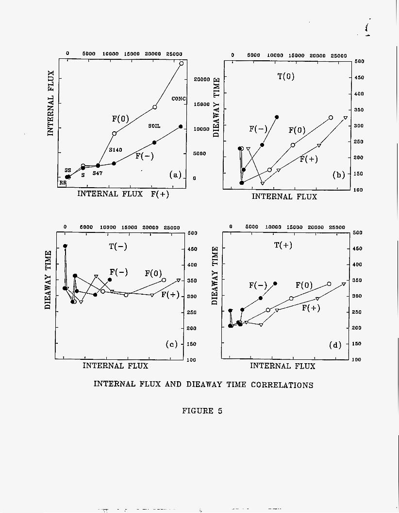
Fig. 5 shows some of these details in a different way. Fig. 5a shows the correlation between

flux measured in the front section of the drum, F(+), versus the flux in the center of the

drum, F(O), and the flux in the back section, F(-). The three flux profiles are clearly well

correlated. The three other plots show the dieaway time responses in the various sections

of the drum versus the flux results of Fig. 5a. Dieaway times, T(0) and T(+), correlate

well with flux for the four higher-flux matrices but the relationship becomes chaotic for the

three low flux cases. T(-), the dieaway time for the back section of a drum in Fig. 5c,

is not particularly well correlated with the flux magnitudes for any of the matrices - so

much cavity flux has leaked in that one is measuring largely cavity-flux times rather than

matrix- fl ux times.

To determine the appropriate thermal flux response, several EMP parameters are studied.

The most important come from the drum flux monitors (DFM), thermal-neutron flux moni-

tors which are shielded to be sensitive only to the surface of the drum and not to the cavity

walls. Of lesser importance are cavity flux monitors (CFM) which monitor flux in the space

between the drum and the chamber walls but which are not shielded from the walls. In both

cases, the flux measured by these monitors is analyzed for its time dependence in addition

to its magnitude. Fig. 6 shows the correspondence between the internal flux and some of the

external flux monitors, and Fig. 6a identifies the corresponding matrices. There is a very

usable correlation between external flux and internal flux for DFMs in Fig. 6a,b,c and even

for CFMs, though the CFM results in Fig. 6d exhibit some ambiguity. Especially pleasing

is the correlation with the drum core flux, F(O), since one wants the external measure to

correlate well with the totally internal parameter. The correlation with F(-) is acceptable

but somewhat problematical.

An interesting parameter might be the time dependence of the flux monitors, themselves.

Fig. 7 shows the correlation between the internal flux and the dieaway time of the flux

monitors, with matrices identified in Fig. 7c. The prognosis for using the monitor dieaway

times is reasonably good for predicting both F(0) and F(+) as seen in the figure for matrices

from S47up. The scatter in the DFM(4) results in Fig. 7a arise from fitting data with low

couting statistics. The results for F(-) are less clear and are indicative of the care which

must be exercised in order to identify the appropriate gross matrix. For S and below, the

leak-in of cavity flux distorts the results too much for most of the monitor times to be useful.

DFM(6), a monitor viewing the surface of the drum away from the generator, appears to

give interesting and useful results for the low flux matrices.

Since the desired flux response function, Flux( V,, t ) , is a function of the time relative

to the neutron generator pulse, it is important that the time character of the internal flux

' be identified. Ref. 1 discusses how the time variation of this function affects the ability of

the imaging algorithm both to image the core of the drum and to separate out the Fast interference for times under 700~s . Fig. 8 compares the external monitor flux measurements

with the internal flux dieaway times, with matrices identified in Fig. 8a. The DFM results

for S47and above are reasonable for T(0) and T(+). But, as usual, results for the weaker

flux matrices are ambiguous and results for all T(-) data are complicated and confusing. In

this comparison, the CFM time results in Fig. 8d are not nearly as useful as were the CFM flux correlations to the internal flux.

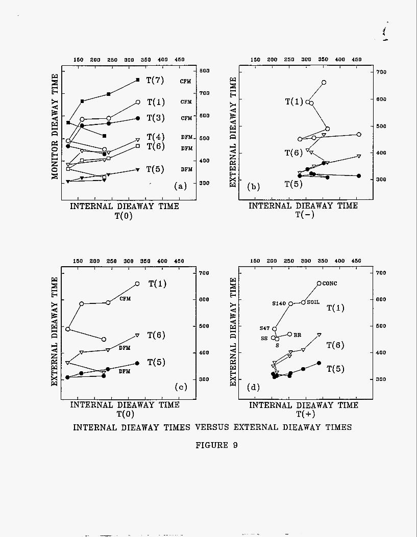
Fig. 9 compares the monitor dieaway times with those of the internal flux. Fig. 9a

compares the dieaway times of six monitors with T(O), the internal dieaway time at the core.

Notice that the CFM monitor times are several hundred microseconds longer than the times

for the DFM due to the longer dieaway time of the cavity. Again, the results are good for

S47 and above, but turn around for the weaker flux matrices. The matrices are identified

in Fig. 9d. The correlation for T(+) in Fig. 9d is also quite good, but there is little if any

simple correlation for T(-) in Fig. 9b. It is likely that pinning down the dieaway time of the

back drum section will require comparing the DFM results to those of the CFM to predict

what the mix of the two flux types is. Fortunately, the DFM results seem to specify the back

section flux fairly well, so specifying the back section dieaway times should be possible.

The dieaway times referred to up till now are single exponential fits to the data. It would

be unreasonable to expect that a single dieaway component is contributing, so this approach

is, at best, an approximation. Ref. 2 will discuss this point in more detail, as it affects the

accuracy with which the flux function can be designated.

Another interesting measure is the amount of the neutron generator pulse which is either

scattered off or transmitted through the drum matrix. The A(d, 0) coefficients in Eq. 2 gives

these measures. A(N2) is a beam transmission measure and A(Sl,S2) is a beam scatter

measure. These measures are of interest since they are the result of interactions with a

primary 14 MeV neutron pulse and not with the much lower energy fission neutrons. An

additional parameter being studied is the time dependence of the signal detectors, since their

response is related directly to the decay time of thermal flux in the drum. Both of these

measures appear to have worthwhile applications, but a detailed discussion of their character

would overwhelm this paper.

SELECTING A MATRIX

Fig. 10 compares the EMP measures for various calibration matrices with measurements

from an actual campaign of drums. Fig. 10a shows the basis for the selection of the matrix

for the efficiency response. The three campaign matrices shown here are soil, concrete rubble,

and Rachig rings. The EMP(SlS2) brightness of soil and Rachig rings is about the same,

near 140%, but the concrete rubble lies at a noticeably higher value, though not as high

as the 165% value for CONC. It seems quite reasonable that the concrete rubble would not

scatter as many neutrons from its surface as would the solid concrete. After the scattering

property is determined, then one looks to the EMP(N2) axis for the transmission value. The

soil matrices lie within the range of the CONC, SOIL, and S147matrices. The concrete

rubble has a somewhat higher transmission, so the appropriate matrix for it, in this case,

would be a combination of the previous three matrices and the 5’47 matrix.

Figs. lOb,c,d show the EMP determination of the calibration matrix for the flux response.

The mock matrices are indicated in the figures along with the campaign matrices. Rachig

rings lie in a clear section of the plot where minimal flux is detected. The concrete rubble

and the soil have different responses, depending on which flux monitor is chosen, but they

would fit a flux response similar to that of SOIL and CONC. In these figures it was possible

to draw a line that follows the increase in the internal flux. This is particularly helpful

when one is dealing with a situation as with DFM(6) in Fig. 10d. Here the mock values

clearly bend around and knowing how to follow the values can be very valuable. DFM(5) is

looking at the generator side of the drum, and DRM(6) is looking at the back of the drum.

The dieaway times for DFM(5) are lower and closer to the actual internal dieaway times.

DFM(6), by looking at the back of the drum, is much more sensitive to the influx of cavity

flux, and it records a somewhat longer dieaway time. The combination of these two measures

enable one to specify the front and back internal flux response as well as to fix the absolute

value of the internal flux. There are difficulties with the actual monitor values which will be

discussed in Ref. 2.

CONCLUSIONS

Since one recognizes the importance of the response functions to the final assay results,

the necessity of a way to specify these functions becomes apparent. The APNea System has

focused on three different but related goals. One goal has been to provide an accurate image,

accurate particularly in relative terms as was discussed in Ref. 1. The companion goal has

been to understand the properties of the APNea Unit and of the drum assay problem so

that mock matrices could be constructed that would supply the appropriate and necessary

response functions. This will not be an easy goal to achieve, since the generating of mock

matrices is a complicated challenge. The final goal has been to provide a defensible method

for identifying the fine-tuned response functions necessary for providing an accurate absolute

image. The EMP methodolgy depends on understanding the internal matrix characteristics

and to relating them to crucial external measures. Within a reasonable dynamic range

of matrices, the EMP methodolgy lays the foundation for an independent identification of

the neutronic characteristics of drums encountered in nondestructive assay situations where

the matrices cannot be directly examined. Determining and understanding the underlying

uncertainties in the final results constitute an exhausting endeavor which will be addressed

in Ref. 2. But the current methodology gives strong optimism that accurate and believable

results can be delivered by a method which is essentially independent of outside crutches.

ACKNOWLEDGMENTS

Larry Pierce was instrumental in fabricating the several mock matrices which were used

in this study. Even though he was not a happy camper when it came time to mix in various

quantities of dusty and rhoking vermiculite, he came up with good methods that provided

quality mock matrices. Jim Madison and Sherry Williams, who are tasked to the daily

operation of the APNea Unit, provided invaluable assistance in obtaining the bulk of the

characteriation and EMP information.

Oak Ridge National Laboratory is managed by Lockheed Martin Energy Systems, Inc.

for the U.S. Department of Energy under contract no. DE-AC05-840R21400. The submitted

manuscript has been authored by a contractor of the U.S. government. Accordingly, the U.S. Government retains a nonexclusive, royalty-free license to publish or reproduce the published

form of the contribution or allow others to do so for US. Government purposes.

REFERENCES

1. D.C. Hensley, “Source Imaging of Drums in the APNea System,” submitted to the

4th Nondestructive Assay and Nondestructive Examination Waste Characterization

Conference, Salt Lake City, Utah (October 24, 1995).

2. D.C. Hensley, “Uncertainty Considerations in the APNea System,” submitted to the

4th Nondestructive Assay and Nondestructive Examination Waste Characterization

Conference, Salt Lake City, Utah (October 24, 1995).

N2 1

w1

8 Segments

Reflector Neutron 1 Generator

N2

30

24

18

12

6

1

Figure: l b ) Schematic view of imaging voxels.

w2

Figure: l a ) 3He tube p lacement in the APNEA.

n

s Ll L1

N z

A I a E u

I V

c3 I4 El s cv z

A I I I I I

!2 w I I I I I V

-10 -5 0 5 10 I I I I I 18000

H=18 co Pv c

6000

4000

2000

0 DRUM RADIUS

-10 -5 0 5 10 I I I I I

3000

1000

300

100

N2 DETECTOR RESPONSE TO AN INTERNAL SOURCE

FIGURE 2

O X 202 40X 80% 80% 100% I 1 1 I I I

n a - rl

0- W

E - o

- 0

0

- t 0

0

0 . 0

0 YTD' HTD

HT'

I ! I I I I I

EMP(N2)

ox 10% 20% 302 40%

SS' 0

S'

O S 0 RR

547'

0 s47

0 SOIL

S140' CONC' ' 0

0 S140

I I I I

EMP(N2)

25000

n 20000 2

c'

z 4 W

15000

10000

5000

D

0 2 lox 20% 30% 402

20000 4

0 4

15000 ';3.' z

10000

5000

0 CONC' 0 SS'

0 S47'

S140' 0 s47

SOIL S140

0 S'

0 O s RR

EMP (N2)

120% 140% 180% I I I

CONC' 0

0 ss

S47' 0 s' 0

RR 0 s 0 . 0

S140'

SOIL 0 s47

S140

I I I

EMP(SlS2)

EMP(N2) AND EMP(S lS2) COMPARED TO N 2 RESPONSES

FIGURE 3

DISCLAIMER

This report w e prepared as an account of work sponsored by an agency of the United States Government. Neither the United States Government nor any agency thereof, nor any of their employees, makes any warranty, express or implied, or assumes any legal liability or responsi- bility for the accuraq, completeness, or usefulness of any information, apparatus, product, or process disclosed, or represents that its use would not infringe privately owned rights. Refer- ence herein to any specific commercial product, process, or service by trade name. trademark, manufacturer, or otherwise does not necessarily constitute or imply its endorsement, recom- mendation, or favoring by the United States Government or any agency thereof. The views and opinions of authors expressed herein do not necessarily state or reflect those of the United States Government or any agency thereof.

8000

7000

6000

5000

8000

7000

6000

5000

-10 - 5 0 5 10 I I I I

-10 -5 0 5 10

DRUM RADIUS INTERNAL FLUX AND DIEAWAY TIMES

FIGURE 4

30000

25000

20000

NG 15000

10000

5000

0

600

500

NG 400

300

200

100

0 5000 10000 15000 20000 25000

I

I I 1 I 1

INTERNAL FLUX F(+)

20000 w r: c 15000 $t

2 4 w 10000 c( n

5000

0

0 5000 10000 15000 20000 25000

1 500

T i 450 4 400

I I I I I I 1100

INTERNAL FLUX

w E

$.

4 W

z i2 E;

0 5000 10000 15000 20000 25000 500

450

400

-f 350

I I I 1 I I I 100 INTERNAL FLUX

0 5000 10000 15000 20000 25000

- (4 I I I I I I

INTERNAL FLUX

INTERNAL FLUX AND DIEAWAY TIME CORRELATIONS

500

450

400

350

300

250

200

150

100

FIGURE 5

0 5000 10000 15000 20000 25000 I I I 1 I l 1800

DFM(4)

- 600

- 400

1 I 1 I I 0 INTERNAL FLUX

0 5000 10000 15000 20000 25000 I I I I I I 7000

DFM( 6)

0 5000 10000 15000 20000 25000

I I 1 1 I I

INTERNAL FLUX

0 5000 10000 15000 20000 25000 8 1 I I I I 120000

CFM( 7)

100000

80000

60000

I 1 I I I I I I 40000 INTERNAL FLUX

INTERNAL FLUX VERSUS EXTERNAL FLUX

FIGURE 6

;i

z - +I M w - Z

r

x -

L - z

EXTERNAL DIEAWAY TIME Ull 1 I -

- 0 ra

u - 0

0 0 2 - W

z - E - 2

c 0

- 0

4 M

N 0 0 0 0

0 0 0

cn 0 0

r

x - n

- 0 W

% w w P 0 en 0

0 0 0 0

I - 0

u - 0

0 0

c u- o" p w o 0 l - g n e

O

N 0

- 0 0 0

N - u - 0

0 0

EXTERNAL DIEAWAY TIME I I I I

- 0

u n - 0

0 W 0

r I

c

4 - g w o 0

N 0

- 0 0 0

N u 0 0 0

+ W

m 0 0

0

r

x - z n a W

UI 0) 0 0 0 0 0

;3 d x

EXTERNAL DIEAWAY TIME I I

- 0

UI - 0

0 0

W I- U - Z O

% i o K c . c p - z

\ n a

- 0

N 0 0 0 0

N UI

- 0 0 0

n + W

n - P

W

I Q

w 0 0

4

n d W

Ilr 0 0

cn 0 0

- m 0 0

n I

W

I I

0 0 0

I 0 UI 0

i

EXTERNAL FLUX : n

0 e n

c 0 0

N 0 0

0 0 0

L 0 0

- P I - P\

EXTERNAL FLUX

I- 0 0

N 0 0

0 0 0

lb 0 0

O c N W P r n m 4 1 0 0 0 0 0 0 0

0 0 0 0 0 0 0 0 0 0 0 0 0 0

o ~ ~ m r n e ~ ~ . ~ 0 0 0 0 0 w P m 0 0 0 0 0 0 0 0

0 0 0 0

EXTERNAL FLUX c3 n n

a 0 W

W

c m o) c c 0 0 0 0 N 0 0 0 0 0 0 0 0 0 0 0 0 0 0 0

0 0

I- O 0

N 0 0

0 0 0

P 0 0

O r N W c m m < 0 0 0 0 0 0 0

0 0 0 0 0 0 0 0 0 0 0 0 0 0 0 0 0 0 0

0 0

EXTERNAL FLUX I 1 1 1 1 1

n d W

c3

W 1 . I 1 1 1 1 1

c 0 0

N 0 0

0 0 0

JI 0 0

160 200 260 300 350 400 460 150 200 250 300 350 400 450

CFM

CFM

DFM

DFM

DFM

(4 I I I 1 I I I I

INTERNAL DIEAWAY TIME T(O)

800

700

600

500

400

300

150 200 250 300 350 400 450

700

600

500

400

T(5) 1 3 0 0

I I I 1 I I 1 I INTERNAL DIEAWAY TIME

T(O)

I 1 I I I

I I I 1 , t I

INTERNAL DIEAWAY TIME T(-)

150 200 250 300 350 400 450

...& RR ss /" T(6) 6 T(5)

s

I I I I I I I

INTERNAL DIEAWAY TIME T(+)

i J

700

000

500

400

300

700

600

500

400

300

INTERNAL DIEAWAY TIMES VERSUS EXTERNAL DIEAWAY TIMES

FIGURE 9

c\ u h

rn 7 - W E

$I-

4 W z1

W

E

U

0 10 20 30

n z E

w - w E

$.-

2 -4 w n

40

I I I I I 800

-

RR

I I I

-

-

-

(4

CONC 0

700

600

500

SS' 0

CONC

5147 S147' 0

SOIL

BLE

I I I

EMP(N2)

50 180

160

140

120

CONC 0

& CONC

I I I I I I I 400 CFM( 1)

20000 40000 60000 80000

I I I I I

V

RR

(b) I I 1 I I

DFM(5)

2000 4000 6000 8000 10000 1 I I I I

CONC

RR 0

0 .3 @ti

CONC O0 0 0

w' SOIL

450

400

350

300

!SO

600

500

100

Efficiency a n d Flux Matrix De te rmina t ion

Figure 10