automated visual direction ldrd 38623 final...
TRANSCRIPT

SANDIA REPORT
SAND2004-6198 Unlimited Release Printed January 2005 Automated Visual Direction LDRD 38623 Final Report
Robert J. Anderson
Prepared by Sandia National Laboratories Albuquerque, New Mexico 87185 and Livermore, California 94550 Sandia is a multiprogram laboratory operated by Sandia Corporation, a Lockheed Martin Company, for the United States Department of Energy�s National Nuclear Security Administration under Contract DE-AC04-94AL85000. Approved for public release; further dissemination unlimited.

Issued by Sandia National Laboratories, operated for the United States Department of Energy by Sandia Corporation.
NOTICE: This report was prepared as an account of work sponsored by an agency of the United States Government. Neither the United States Government, nor any agency thereof, nor any of their employees, nor any of their contractors, subcontractors, or their employees, make any warranty, express or implied, or assume any legal liability or responsibility for the accuracy, completeness, or usefulness of any information, apparatus, product, or process disclosed, or represent that its use would not infringe privately owned rights. Reference herein to any specific commercial product, process, or service by trade name, trademark, manufacturer, or otherwise, does not necessarily constitute or imply its endorsement, recommendation, or favoring by the United States Government, any agency thereof, or any of their contractors or subcontractors. The views and opinions expressed herein do not necessarily state or reflect those of the United States Government, any agency thereof, or any of their contractors. Printed in the United States of America. This report has been reproduced directly from the best available copy. Available to DOE and DOE contractors from
U.S. Department of Energy Office of Scientific and Technical Information P.O. Box 62 Oak Ridge, TN 37831 Telephone: (865)576-8401 Facsimile: (865)576-5728 E-Mail: [email protected] Online ordering: http://www.osti.gov/bridge
Available to the public from
U.S. Department of Commerce National Technical Information Service 5285 Port Royal Rd Springfield, VA 22161 Telephone: (800)553-6847 Facsimile: (703)605-6900 E-Mail: [email protected] Online order: http://www.ntis.gov/help/ordermethods.asp?loc=7-4-0#online
2

SAND2004-6198Unlimited Release
Printed January 2005
Automated Visual DirectionLDRD 38623 Final Report
Robert J. AndersonMobile Robotics DepartmentSandia National Laboratories
P.O. Box 5800Albuquerque, New Mexico 87185-1125
Abstract
Mobile manipulator systems used by emergency response operators consist of an articulated robot arm, a remotely driven base, a collection of cameras, and a remote communications link. Typically the system is completely teleoperated, with the operator using live video feedback to monitor and assess the environment, plan task activities, and to conduct the operations via remote control input devices. The capabilities of these systems are limited, and operators rarely attempt sophisticated operations such as retrieving and utilizing tools, deploying sensors, or building up world models. This project has focused on methods to utilize this video information to enable monitored autonomous behaviors for the mobile manipulator system, with the goal of improving the overall effectiveness of the human/robot system. Work includes visual servoing, visual targeting, utilization of embedded video in 3-D models, and improved methods of camera utilization and calibration.
3
Acknowledgements
The work presented in this report represents a summary of work conducted in the last three years, with an emphasis on the most recent year’s work. Many Sandians and Sandia contractors contributed to the work presented within this report and should be acknowledged. Hanspeter Shaub and Chris Smith developed much of the visual snake algorithms used. Eric Gottlieb, Fred Oppel and others invented the Umbra software environment that was heavily utilized throughout this project. Dan Small developed the live video input capability within the Umbra framework. Mike McDonald generated much of the original Active Sketch code, based off of targeting code developed by Chris Wilson. Michael Saavedra developed the zoom camera housing and helped to keep much of the hardware running. Scott Gladwell developed planners that converted active sketch commands into robot actions. Phil Bennett provided the problems, the motivation and the customers to keep us focused on real tasks.
4

CONTENTS
ABSTRACT ............................................................................................................3
1 INTRODUCTION .........................................................................................7
2 AUTOMATIC TOOL PICK-UP WITH VISUAL SERVOING ............... 82.2 Statistical Pressure Snakes............................................................................ 82.3 Using Snakes For Tool-Pickups ................................................................... 92.4 Improving Tracking Reliability ..................................................................102.5 Implementation Details ...............................................................................102.6 Stages of Automated Visual Servoing ........................................................11
3 VISUAL TARGETING AND ACTIVE SKETCH ...................................133.1 Visual targeting ...........................................................................................133.2 Active Sketch ..............................................................................................133.3 Implementing Automatic Motion Behaviors ..............................................14
4 EMBEDDING VISUAL INFORMATION ...............................................17
5 IMPROVING CAMERA CALIBRATION .............................................185.1 Intrinsic Camera Calibration and the Distortion Model ............................. 185.2 Extrinsic Calibration and the Camera Calibration Tool .............................195.3 The Non-Perspective Pose Estimation Problem ......................................... 215.4 The Calibration Transform Loop................................................................ 225.5 Developing an Interactive Pose Estimation Tool ....................................... 235.6 Digital Zoom Camera Calibration .............................................................. 24
6 CONCLUSIONS ......................................................................................... 27
REFERENCE........................................................................................................28
APPENDIX A: CAMERA CALIBRATION TERMINOLOGY .........................29
APPENDIX B: USING THE EXTRINSIC/INTRINSIC REFERENCE MODEL32
APPENDIX C: SOLVING THE NON-PERSPECTIVE N-POINT PROBLEM 35
APPENDIX D: XML FORMAL FOR ZOOM CAMERA CALIBRATION ......39
DISTRIBUTION ..................................................................................................41
5

6

1.0 Introduction
Mobile manipulator systems, such as the RemotecAdvanced Manipulator (Figure 1) are used by emergencyresponse personnel to respond to threats posed by impro-vised explosive devices (IEDs). Existing commercial sys-tems are limited in their autonomous capability becausethey rely solely on operator interpretation of the live videoimages and direct operator control of the manipulator, i.e.,teleoperation. With this LDRD we have focused on devel-oping techniques to reduce the burden on the operator bydigitally sampling the live video image and developingalgorithms that use this information to semi-autono-mously control the remote manipulator system. The mobile response systems that have been considered,are all similar in setup. A remote vehicle is operated outof direct line of sight of the operator. A live video feed isbrought back to an operator console similar to one shownin Figure 2 and captured on a frame grabber attached to the operator control unit. Snapshots of thisvideo can be taken, and/or the live video stream used directly.A large number of tasks related to the utilization of video in the remote control of emergencyresponse vehicles have been conducted during the course of this LDRD. Automatic tool pickupshave been demonstrated using visual servoing algorithms based on statistical pressure snakes. Thealgorithms have proven to be robust despite the unstructured lighting conditions. The remotemanipulator is able to visually servo based off of the snake inputs to automatically grasp tools.This work is described in section 2.0. Visual servoing uses the continuous live video feed from the wrist camera. Visual targeting, on theother hand, utilizes a pair of snapshotsfrom a pair of calibrated cameras.Visual targeting and active sketch tech-nology have also been further developedwithin this project. With the activesketch framework simple primitives areused in a pair of stereo images. Select-ing these primitives enables a set of pos-sible actions for the operator to choosebetween. The latest active sketch imple-mentations are described in section 3.0. Embedded video provides context forlive video information and allows a cor-relation between live video data and vir-tual representations of the world. Workin embedded video for mobile responsesystem is described in section 4.0.Camera calibration is crucial for converting image data to robot action. Section 5.0 documentsdevelopments in camera calibrations, including the latest developments utilizing calibrated zoomcamera systems.
Figure 1: Remotec Advanced manipulator with target head
Figure 2. Remote Manipulator Operator Console
7

2.0 Automatic Tool Pick-Up With Visual Servoing
An emergency response robotic operator can deploy a wide variety of tools, depending on the taskat hand. Grappling hooks, explosive tools, X-ray equipment, chemical sniffers, small drills etc.,might all be utilized. In many cases, thesemay be picked up from a trailer, or from asecondary pack-mule robot, and the loca-tion of these tools with respect to the robotcannot be precisely known. Figure 3 illus-trates the retrieval of tools from a pack-mule robot.Teleoperating a tool grasp can be a slowprocedure, since the position and orienta-tion of the tool must be controlled pre-cisely to prevent damage to the tool or thetool holder. The tools themselves, how-ever, can be engineered for easy recogni-tion and retrieval. Tool grasps, aretherefore, an excellent candidate for auto-mation. In this section we describe how wehave utilized statistical pressure snakesand visual servoing to demonstrate auto-matic visual grasping for telerobotic sys-tems.
2.1 Statistical Pressure Snakes
Our approach to visual servoing utilizes statistical pressure snakes, based on the Perrin-Smithmodel [1]. A pressure snake is a mathematical construct representing a closed loop segmentedcontour on an image plane. The snake’s length and position is constantly being pushed by imagepressures, as it seeks to find a minimum energy solution. Regions of the image with a “good” fea-ture, such as its measured closeness to a desired color generate pressures that push out the snakefrom its interior, while contour tension tries to collapse the contour. Snakes can be initiated byeither starting at an initial selection point and growing the snake outward, or by using the entireregion and collapsing the snake around a region. In either case when the snakes are well tuned,they should expand or contract to follow the contours of a shape of interest after a few iterations.Snakes provide many advantages over other image processing techniques. First, the algorithm isfast. The computations are typically of order n, where n is the number of segments in the snake.This number can shrink or grow depending on the overall length of the snake contour, but is stillsmall compared to the image size. Only a small window of pixels around each vertex is all that isused for image analysis in a given iteration. Second, the snake allows for easy interaction with theuser. A simple button click can define a seed-region for growing a new snake. The evolution of thesnake algorithm is easily displayed by overlaying a snake drawing on the live video, so the opera-tor can monitor operations in real-time. The snake data structure can be queried for essential objectfeatures such as center, size and orientation, which can be used to drive the visual servoing opera-tions.
Figure 3: Pack-Mule Retrieval of Tools
8

The development of color based statistical pressure snakes under this LDRD has been well docu-mented in number of SAND reports and conference proceedings. [2-7]
2.2 Using Snakes For Tool-Pickups
Snakes help to define a region of interest for the robot system, but do not directly result in any use-ful operations. To become truly useful for the mobile manipulator system, information derivedfrom the snakes must be utilized as one part of a motion planning algorithm. In a completelyunstructured environment this is difficult, since the robot system has no method to transform gen-eral object contour information into a plan of action. By constraining the problem and controlling apart of the environment, however, a automated activity for the mobile manipulator can be devel-oped. This has been done for tool pickups.Industrial robots commonly pick up tools without visualservoing simply by moving to a series of pre-taught points.Mobile manipulator systems, on the other hand, typicallylack the structure and the precision required to pick uptools open loop. In many cases tools pickup locations areimprovised, tools are placed on trays or on tool racks with-out precise alignment locations. Tools may be deliveredoff of a mobile pack-mule, or retrieved from the back of atool trailer, without any precision a priori location infor-mation available to the robot. Mobile manipulators tend tobe less rigid, with more mechanical play and less accuratejoint calibration, so even if the tool position is preciselyknown, an open loop attempt to grab a tool may fail evenif the tool location with respect to the robot is preciselyknown. Industrial robots also work in a workcell wherehumans, and their corrupting influences are avoided. Toolsare always located in the same locations, because no-onewas allowed to move them away. Emergency response robots, however, work closely with humanoperators, and are thus subject to the whims of operators to move and deploy different tools.To enable automated tool pick-ups, we add a level of structure to the tools themselves. In particularwe place a colored rectangular patch at a known position and location offset from the tool pickuppoint. This patch is designed so it will be completely viewable from the gripper camera during theentire approach sequence. Figure 4 shows a colored patch attached to a telemanipulator tool, inthis case an X-ray source. By standardizing the distance and size of the rectangular patch, we candirectly convert the information gleaned from the active snake, to a motion plan to pick up a tool.Since the size of the rectangular patch is known a priori, the measured area in pixels of theenclosed snake contour maps directly to an absolute distance to the target. The principal axes ofthe rectangular block can be used for orientation alignment, and the center of the target is used todetermine the amount of translation needed. Thus a single rectangular block can be used to deter-mine four degrees-of-freedom of motion: x, y, z translation, and roll orientation in the image frame.In addition, by controlling the color of both the rectangular patch and its background, an extremelyrobust snake can be obtained.Pitch and yaw errors in the image plane for the rectangular block also result in skewing of the sidesof the rectangle, but the measurement sensitivity to pitch and yaw is far less than for the otherparameters and was not used.1 In practice, tools are oriented so that a standard vertical approach
Figure 4: Standardized Tool Pickup on an X-Ray source tool
9
is needed to make the grab, and no additional orientation alignment other than roll is needed. Onlyif the robot is operating in very hilly terrain and neither the robot nor the tool caddy can be placedon the same slope is this seen as a problem.
2.3 Improving Tracking Reliability
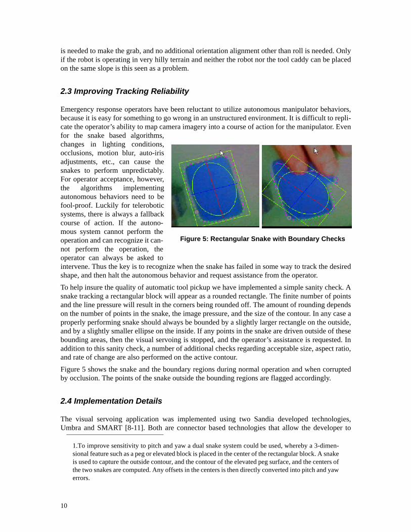
Emergency response operators have been reluctant to utilize autonomous manipulator behaviors,because it is easy for something to go wrong in an unstructured environment. It is difficult to repli-cate the operator’s ability to map camera imagery into a course of action for the manipulator. Evenfor the snake based algorithms,changes in lighting conditions,occlusions, motion blur, auto-irisadjustments, etc., can cause thesnakes to perform unpredictably.For operator acceptance, however,the algorithms implementingautonomous behaviors need to befool-proof. Luckily for teleroboticsystems, there is always a fallbackcourse of action. If the autono-mous system cannot perform theoperation and can recognize it can-not perform the operation, theoperator can always be asked tointervene. Thus the key is to recognize when the snake has failed in some way to track the desiredshape, and then halt the autonomous behavior and request assistance from the operator. To help insure the quality of automatic tool pickup we have implemented a simple sanity check. Asnake tracking a rectangular block will appear as a rounded rectangle. The finite number of pointsand the line pressure will result in the corners being rounded off. The amount of rounding dependson the number of points in the snake, the image pressure, and the size of the contour. In any case aproperly performing snake should always be bounded by a slightly larger rectangle on the outside,and by a slightly smaller ellipse on the inside. If any points in the snake are driven outside of thesebounding areas, then the visual servoing is stopped, and the operator’s assistance is requested. Inaddition to this sanity check, a number of additional checks regarding acceptable size, aspect ratio,and rate of change are also performed on the active contour. Figure 5 shows the snake and the boundary regions during normal operation and when corruptedby occlusion. The points of the snake outside the bounding regions are flagged accordingly.
2.4 Implementation Details
The visual servoing application was implemented using two Sandia developed technologies,Umbra and SMART [8-11]. Both are connector based technologies that allow the developer to
1.To improve sensitivity to pitch and yaw a dual snake system could be used, whereby a 3-dimen-sional feature such as a peg or elevated block is placed in the center of the rectangular block. A snakeis used to capture the outside contour, and the contour of the elevated peg surface, and the centers ofthe two snakes are computed. Any offsets in the centers is then directly converted into pitch and yawerrors.
Figure 5: Rectangular Snake with Boundary Checks
10

combine system modules to implement behaviors. Umbra is focused on graphics, visualization,and operator interaction. SMART is used for real-time servo control and teleoperation. Together,they provide a rich environment for advanced robotic systems.
Figure 6 Umbra Modules Used for Implementation
Figure 6 shows the icon representation of the relevant Umbra components in the system. An ACTIVE_SKETCH module provides a connection to the live camera frame grabber (via a DigiCam Umbra module). The vsSnake module uses the image connector as an input and implements the snake algorithm. The vsServo module takes the snake inputs and generates a velocity error command to drive the robot’s tool. The UMB_REG module provides a direction socket connection between Umbra’s connectors and SMART’s data registers, allowing the servo error command to directly drive the embedded robot controller. Finally, the USG_VIEWER is used to embed an Umbra scene graph visualizer within the application.
Figure 7 SMART Modules Used for Visual Servoing Implementation
Figure 7 shows the icon representation of the SMART modules used in the system. The REG_VEL receives the velocity error commands from the UMB_REG module. The ROTATE_KIN module rotates the velocities into the tool reference frame, the WOLVERINE_KIN converts tool speeds into joint speeds, and the WOLVERINE_JNTS module drives the robot.
2.5 Stages of Automated Visual Servoing
The visual servoing process for an automated tool grab is illustrated in Figure 8. First the robot ismoved to a point above the expected location of the tool. Initial snake acquisition is obtained byeither the operator clicking on the colored patch on the tool and growing the snake outward, or byshrinking a snake around the entire region until it collapses on the tool region of interest. Once avalid tool patch has been acquired, the visual servoing stage begins. During visual servoing the 4-
11
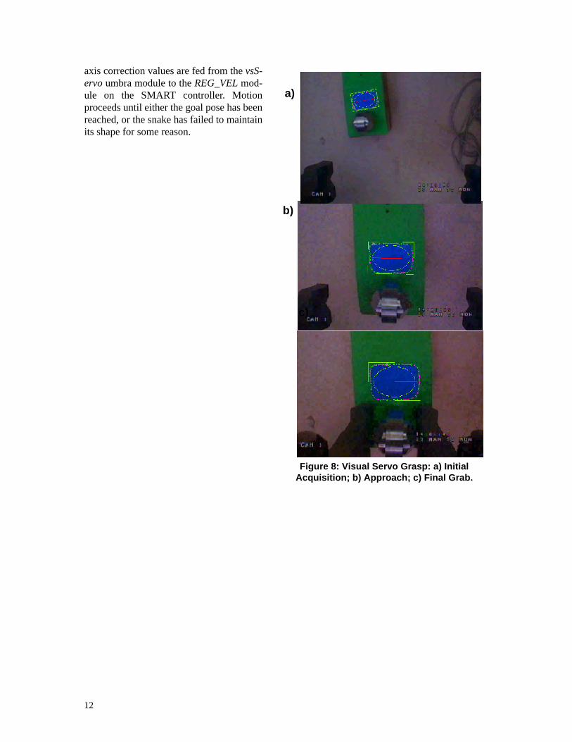
axis correction values are fed from the vsS-ervo umbra module to the REG_VEL mod-ule on the SMART controller. Motionproceeds until either the goal pose has beenreached, or the snake has failed to maintainits shape for some reason.
Figure 8: Visual Servo Grasp: a) Initial Acquisition; b) Approach; c) Final Grab.
a)
b)
c)
12

3.0 Visual Targeting and Active Sketch
Active Sketch and Visual Targeting have been the mainstay technologies for developing autono-mous behaviors for mobile manipulators. Although they were invented within prior researchprojects, they have been heavily utilized, developed and refined during the course of this project.In this section we define these approaches and document their current implementation as appliedto mobile robot control.
3.1 Visual targeting
Visual Targeting provides the basis for the more operation focused Active Sketch techniques, andhas been utilized by robotics researchers for years [13] Targeting requires a pair of calibrated cam-era snapshots to be taken of a common object viewed from different angles. Typically this is doneusing a calibrated stereo camera head, with snapshots being taken simultaneously, but this isn’talways the case. As an example, Figure 9 shows a Sandia developed stereo targeting head containing two fixedfocal length cameras mounted on a pan-tilt-unit, which is attached to a mast that is in turn attachedto the robot torso. The operator moves the PTU with a joystick to point both cameras at a target ofinterest, and then clicks a button to take a pair of snapshots.
The user then selects a common feature in bothimages. Using the mathematics of the calibratedcamera model, each pixel selected in space corre-sponds to a vector cast in 3-dimensional space.The pair of vectors from the two images corre-spond to a unique point in 3-D space, ideally thepoint of intersection of the two vectors, but moretypically due to image and calibration errors thepoint of nearest intersection of the two skew vec-tors. In summary, visual targeting simply uses tri-angulation of two calibrated camera images toodetermine the 3-D position of a point in space withrespect to the robot. And a feature so selected isconsidered “targeted”.
3.2 Active Sketch
Visual targeting in itself does not specify robotaction. All it specifies is the 3-D point of a featurein the robot’s workspace. For a robot to performan automatic action, however, much more infor-mation must be available. A robot task requiresmuch more than the 3-D position of a feature in
space. It requires a complete goal pose, consisting of a desired 6-DOF position and orientation ofthe robot’s gripper. It also requires an approach path, the series of joint angles that will safely takethe robot from its current location to the goal pose.
Figure 9: Visual Targeting Head on a Remotec Advanced Mobile Manipulator
13

The Active Sketch technology was developed at Sandia, [14,15] to bridge the gap between 3-Dposition targeting and robot action. With Active Sketch, the task is divided into two steps, theobject specification and the task specification. In our implementation, the available object specifi-cation tools are simple geometric primitives: a point, a line, two connected lines representing aplane, and three lines with a common vertex used to define a volume called a triad. Selecting thetool places a copy of the geometric primitive into both images, where they can be dragged to alignwith common features in the image plane. Rather then forcing the operator to completely match image features at each vertex, however,Active Sketch, utilizes the epi-polar constraint to substantially simplify the stereo matching prob-lem. The epi-polar constraint is a realization that the ray cast by selecting a pixel in a target image,corresponds to a line when viewed from a second range image. By limiting mouse selections inthe range image to points that lie along the constraint line, the search process becomes a onedimensional selection rather than a two dimensional selection. Not only is the likelihood of theoperator selecting the wrong feature substantially diminished, it is also possible to find alignmentseven when targets are completely occluded in the second image.
Figure 10 Stereo Snapshots of a pipe.One of the object specification tools are placed in the image plane, e.g., point tool, line tool, planetool, and triad tools, and then moved in alignment with common features in both images. Selectingand highlighting the object makes available a set of actions. An intelligent planner then uses the 3-D location data as a starting point for planning a path to execute the desired action. Figure 10shows a pair of stereo images taken within Active Sketch. A line tool if being used by the operator,and has been dragged over the features of interest, namely the axis of the pipe bomb.
3.3 Implementing Automatic Motion Behaviors
Figure 11 below shows a typical trajectory task control panel used for mobile manipulation. Itworks intimately with the Active Sketch environment. As different active sketch primitives arechosen, i.e., points, lines or surfaces, different motion macros become available. When no featureshave been selected only the fixed, “Canned Motion” routines are allowed. If a line tool is chosen,macros such as “Grab Pipe” or “Move Around Axis” become selectable.
14

Figure 11 Automated Control PanelThe automatic control panel also includes a large “VCR” controller. Play begins automaticallywhen a trajectory macro has been selected. The operator is free to pause, backup, change speeds,and resume motion as needed, simply by clicking on the interface buttons.For example, to grab a pipe, the operator first aims the stereocamera system at the pipe of interest, and takes the pair of snap-shots as in Figure 10. A Line tool is selected and dragged acrossthe image. Once the line is selected a series of line-based trajec-tory macros becomes available to the operator, as in Figure 12.By clicking on the appropriate button, the “Grab Pipe” motionplanner is called, and a path to grab the center of pipe from aboveis planned and initiated. The cameras are automatically slewedover to directly monitor the operation and the robot starts to exe-cute the planned motion. The operator monitors the motion, and ifneeded, can pause or add position corrections. A door opening task can be conducted in much the same fashion.In this case the line of interest is the hinge line of the door and the“Move Around Axis” button should be selected. Thisplanner will apply the right hand rule to the axis andsweep out an arc around the axis, starting with the robotscurrent grip point. Figure 12: Operator Line
Tool Macros
15
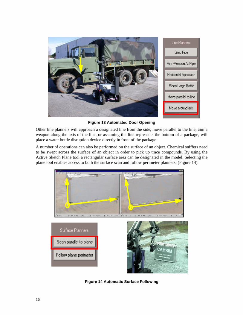
Figure 13 Automated Door OpeningOther line planners will approach a designated line from the side, move parallel to the line, aim aweapon along the axis of the line, or assuming the line represents the bottom of a package, willplace a water bottle disruption device directly in front of the package.A number of operations can also be performed on the surface of an object. Chemical sniffers needto be swept across the surface of an object in order to pick up trace compounds. By using theActive Sketch Plane tool a rectangular surface area can be designated in the model. Selecting theplane tool enables access to both the surface scan and follow perimeter planners. (Figure 14).
Figure 14 Automatic Surface Following
16

4.0 Embedding Visual Information
Another problem inherent in the utilization ofremote cameras is the tunnel vision phenomena.Operators lose spatial awareness of the live videofeed and are often unable to correctly interpretimagery. By embedding visual information within a3-D modelling environment this problem can belargely averted. During the course of this LDRD a number of visu-alization tools have been added to the system. Livecamera imagery has been embedded in correspon-dence with the graphical model, and video imageryis cast onto an embedded video screen. The opera-tor is able to change the level of transparency ofthe live video feed to move between live viewsand virtual views as needed.Image snapshots can also be taken and embeddedwithin the working model. Each snapshot has aworking image frustum associated with it whichcan be visually displayed. The images can be viewed from the original camera position and orien-tation, or from any other location. Figure 15 shows a pair of snapshots taken of a box from a dif-ferent points of view.The active sketch tool can be used to add geometry to the scene graph. By using the triad tool, boxshaped objects can be readily placed and visualized within the virtual world. This not only helpskeep the operator informed of objects in the robot’s workcell, but it also serves as a forensics tool,to help build up a working model of the robot’s environment. Figure 16 shows a box that has beenadded to the scene graph via the active sketch interface. The semi-transparent image lines up withthe 3-D geometry when viewed from the camera’s point of view.
Figure 16 Semi-Transparent Video overlay over a modeled box
Figure 15: Embedded Visual Model
17

5.0 Improving Camera Calibration
For the robot system to be able to perform operations semi-autonomously, precise 3-D measure-ments must be directly obtainable from the video feedback, and correlated from multiple cameraviews. This task is called camera calibration, and involves determining the mapping betweenimage plane coordinates and 3-D space. Good camera calibration is crucial for visually directedmobile manipulation systems. Appendix A summarizes the terminology and algorithms used forcomputing the calibration of a fixed focal length camera. Appendix B describes the decompositionof the camera calibration matrix into intrinsic and extrinsic representations.Mobile manipulator systems typically have a suite of cameras: a drive camera, a reverse camera,one or two wrist cameras, and a torso mounted pan and tilt targeting head. For visual targeting sys-tems, camera calibration has typically involved accurately calibrating a stereo pair of fixed focallength targeting cameras. These cameras are taken to a precision optical bench, where both intrin-sic and extrinsic camera parameters are measured and recorded. The calibrated stereo camera sys-tem is then attached to the robot, and the position offset is measured. Unfortunately, our experience with applying calibrated camera heads to mobile manipulation hasuncovered a number of problems with this approach. Off-line camera calibration works well in alab environment, but in the field, cameras are too easily jostled and moved from initial setup posi-tions. Small orientation alignment errors can lead to relatively large targeting errors. Cameramount points may change or degrade over time. All of this leads to error buildup for targetingoperations. The single stereo head is also problematic. To fit within the footprint of the robot, the spacing ofstereo cameras is typically ten inches or less. This small spacing reduces the accuracy of distancemeasurements. A torso mounted camera may also have issues with arm occlusion. The arm oftenneeds to be rotated out of the way for the targeting operations to succeed, reducing the both theoperational speed and advantages of autonomous operations. In addition, remaining cameras,such as drive, reverse and wrist cameras, are under-utilized. These cameras could provide valuableinformation from a different perspective, if calibration for randomly mounted cameras werestraight-forward. Camera calibration has, to date, relied on fixed focal length cameras. Unfortunately without zoomcapabilities, these cameras have limited utility. They work well for targeting operations on objectswith measurable features between 4” and 20” in length, but are unable to adequately target smallfeatures such as key-holes, or large features such as shipping crates, packages or buildings.This research project has begun to address these issues, but the work has not been completed. Wehave developed an interactive tool for calibrating cameras using a benchtop fixture. We havedeveloped a new algorithm for pose estimation which should ultimately allow improved in situcamera calibration. We have partially developed an interactive graphics tool for pose estimationwhich makes it possible to use any known geometric object as a possible calibration tool. We’vebegun to integrate calibrated zoom cameras into our environments and have developed a calibra-tion approach for these cameras. This section describes these most recent developments.
5.1 Intrinsic Camera Calibration and the Distortion Model
There is a significant body of work in camera calibration [16-18]. Typically camera calibration canbe divided into three stages, intrinsic and extrinsic calibration, and pose estimation. Intrinsic cali-bration involves the measurement of camera focal lengths, camera distortion, and pixel offsets.
18
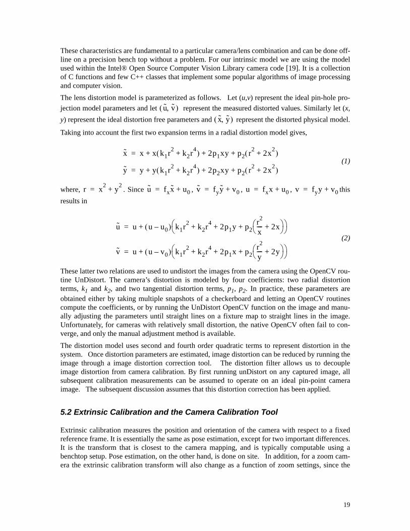
These characteristics are fundamental to a particular camera/lens combination and can be done off-line on a precision bench top without a problem. For our intrinsic model we are using the modelused within the Intel® Open Source Computer Vision Library camera code [19]. It is a collectionof C functions and few C++ classes that implement some popular algorithms of image processingand computer vision. The lens distortion model is parameterized as follows. Let (u,v) represent the ideal pin-hole pro-jection model parameters and let represent the measured distorted values. Similarly let (x,y) represent the ideal distortion free parameters and represent the distorted physical model.
Taking into account the first two expansion terms in a radial distortion model gives,
(1)
where, . Since , , , thisresults in
(2)
These latter two relations are used to undistort the images from the camera using the OpenCV rou-tine UnDistort. The camera’s distortion is modeled by four coefficients: two radial distortionterms, k1 and k2, and two tangential distortion terms, p1, p2. In practice, these parameters areobtained either by taking multiple snapshots of a checkerboard and letting an OpenCV routinescompute the coefficients, or by running the UnDistort OpenCV function on the image and manu-ally adjusting the parameters until straight lines on a fixture map to straight lines in the image.Unfortunately, for cameras with relatively small distortion, the native OpenCV often fail to con-verge, and only the manual adjustment method is available.The distortion model uses second and fourth order quadratic terms to represent distortion in thesystem. Once distortion parameters are estimated, image distortion can be reduced by running theimage through a image distortion correction tool. The distortion filter allows us to decoupleimage distortion from camera calibration. By first running unDistort on any captured image, allsubsequent calibration measurements can be assumed to operate on an ideal pin-point cameraimage. The subsequent discussion assumes that this distortion correction has been applied.
5.2 Extrinsic Calibration and the Camera Calibration Tool
Extrinsic calibration measures the position and orientation of the camera with respect to a fixedreference frame. It is essentially the same as pose estimation, except for two important differences.It is the transform that is closest to the camera mapping, and is typically computable using abenchtop setup. Pose estimation, on the other hand, is done on site. In addition, for a zoom cam-era the extrinsic calibration transform will also change as a function of zoom settings, since the
u v,( )x y,( )
x x x k1r2 k2r4+( ) 2p1xy p2 r2 2x2+( )+ + +=
y y y k1r2 k2r4+( ) 2p2xy p2 r2 2x2+( )+ + +=
r x2 y2+= u fxx u0+= v fyy v0+= u fxx u0+= v fyy v0+=
u u u u0–( ) k1r2 k2r4 2p1y p2r2
x---- 2x+⎝ ⎠⎛ ⎞+ + +⎝ ⎠
⎛ ⎞+=
v u u v0–( ) k1r2 k2r4 2p1x p2r2
y---- 2y+⎝ ⎠⎛ ⎞+ + +⎝ ⎠
⎛ ⎞+=
19

effective center of the camera model changes as a function of zoom. The pose estimation, shouldbe constant as a function of zoom setting. Figure 17 shows a interface tool that has been developed to calibrate cameras using a bench topfixture. Both the intrinsic and extrinsic parameters of the cameras can be calibrated with this tool,but not the final camera pose estimation. The intrinsic parameters can be computed in one of twomethods: the native method within OpenCV which takes a series of pictures of checkerboards andcomputes distortion parameters, and the fixture based method which computes the pin-hole cam-era model intrinsic parameters, and allows the distortion to be determined interactively.
Figure 17 Fixture based Camera Calibration Tool
20

The method requires a camera fixture containing a series of measured points. The points must not all be co-planar. In practice we have used either a series of posts on a precision optical bench, or a calibration fixture with a sliding panel containing a grid of known points. (see Figure 18)
Figure 18 Calibration Fixture with Adjustable depth feature.
5.3 The Non-Perspective Pose Estimation Problem
A camera can be carefully calibrated on a bench top, and then fail when placed on the robot due toinaccuracies in mounting the camera system. For visual targeting to work well, this last transfor-mation needs to be computed accurately. This transform is called the camera pose, and consists ofthe position and orientation of the image device with respect to the robot. The same problemarises when the position and orientation of known objects need to be known with respect to therobot’s position. Pose estimation focuses on just the orientation and position of a device, either a camera or targetedobject. In many cases, the imaging device is a single perspective camera with a single snapshot,with multiple features selected. In this case (assuming the pin-point model of the camera) all ofthe UV selections correspond to rays which all intersect at a common point. If three such well-determined points are selected, then a correct solution can be found algrebraically by solving apolynomial. In general, however, four possible solutions exist, and additional information mustbe used to determine the correct solution. This problem is called the P3P problem.To improve the accuracy of the P3P solution a number of researchers have extended the results toN points (N>3). By using the 3 point solution as an initial seed, further refinement and accuracy isobtained by adding more points to the system. The fourth point is often used to resolve the multi-ple solutions found from solving the algebraic equation. All points must still intersect at a commonpoint, however, for these approaches to work.In tracking operations a target object may have essentially the same perspective distortion over allfeature points. In this case, a weak perspective assumption can be made, and the equations can besimplified substantially. The POSIT algorithm is a highly efficient approach for computing cam-era frames for perspective systems using a weak perspective assumption. A number of general imaging devices (GIDs) don’t fit the perspective camera model, i.e., when theray segments don’t all intersect at a common point. This may occur with high distortion lenses,line cameras, or in our case, due to obtaining pose estimation from multiple camera views, from a
21
camera mounted on a PTU system. The non-perspective n point problem of finding a cameraobject pose is a variation of the PnP (Perspective N Point problem), without a common intersec-tion point [20]. Finding an effective means of solving this problem is critical for robot pose estima-tion for our mobile manipulators. In general, the problem amounts to finding the rotation matrix and translation offset between thecamera system and the object, by establishing a correspondence between objects in the imageframe (i.e., u, v coordinates) and objects in a world frame (x, y, z) coordinates. The rotation/transla-tion can be represented by 6 independent parameters, and thus by defining 3 UV-XYZ correspon-dences a solution for the rotation frame should be attainable.In Appendix D we develop an algorithm for iteratively solving the nPnP problem assuming a goodapproximate value for the rotation and offset has already been obtained. The algorithm is genericand can be used to find any unknown transformation given a sufficient number of image corre-spondences.
5.4 The Calibration Transform Loop
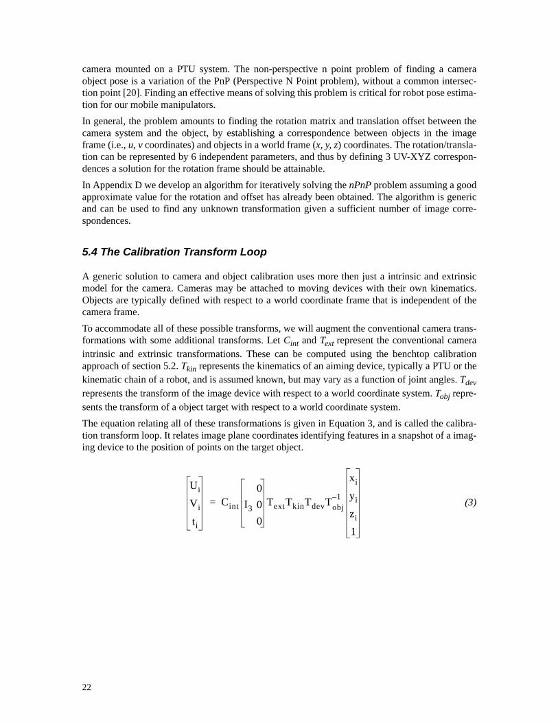
A generic solution to camera and object calibration uses more then just a intrinsic and extrinsicmodel for the camera. Cameras may be attached to moving devices with their own kinematics.Objects are typically defined with respect to a world coordinate frame that is independent of thecamera frame. To accommodate all of these possible transforms, we will augment the conventional camera trans-formations with some additional transforms. Let Cint and Text represent the conventional cameraintrinsic and extrinsic transformations. These can be computed using the benchtop calibrationapproach of section 5.2. Tkin represents the kinematics of an aiming device, typically a PTU or thekinematic chain of a robot, and is assumed known, but may vary as a function of joint angles. Tdevrepresents the transform of the image device with respect to a world coordinate system. Tobj repre-sents the transform of a object target with respect to a world coordinate system. The equation relating all of these transformations is given in Equation 3, and is called the calibra-tion transform loop. It relates image plane coordinates identifying features in a snapshot of a imag-ing device to the position of points on the target object.
(3)
Ui
Vi
ti
Cint I3
000
TextTkinTdevTobj1–
xi
yi
zi
1
=
22
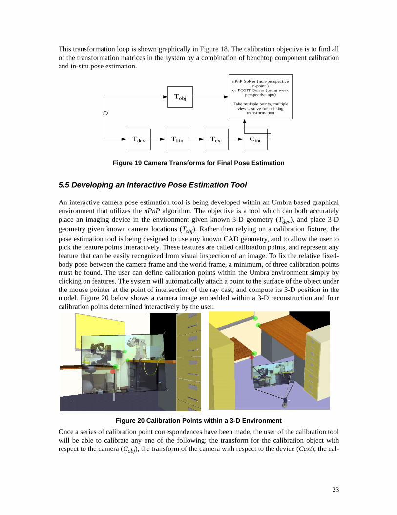
This transformation loop is shown graphically in Figure 18. The calibration objective is to find allof the transformation matrices in the system by a combination of benchtop component calibrationand in-situ pose estimation.
Figure 19 Camera Transforms for Final Pose Estimation
5.5 Developing an Interactive Pose Estimation Tool
An interactive camera pose estimation tool is being developed within an Umbra based graphicalenvironment that utilizes the nPnP algorithm. The objective is a tool which can both accuratelyplace an imaging device in the environment given known 3-D geometry (Tdev), and place 3-Dgeometry given known camera locations (Tobj). Rather then relying on a calibration fixture, thepose estimation tool is being designed to use any known CAD geometry, and to allow the user topick the feature points interactively. These features are called calibration points, and represent anyfeature that can be easily recognized from visual inspection of an image. To fix the relative fixed-body pose between the camera frame and the world frame, a minimum, of three calibration pointsmust be found. The user can define calibration points within the Umbra environment simply byclicking on features. The system will automatically attach a point to the surface of the object underthe mouse pointer at the point of intersection of the ray cast, and compute its 3-D position in themodel. Figure 20 below shows a camera image embedded within a 3-D reconstruction and fourcalibration points determined interactively by the user.
Figure 20 Calibration Points within a 3-D EnvironmentOnce a series of calibration point correspondences have been made, the user of the calibration toolwill be able to calibrate any one of the following: the transform for the calibration object withrespect to the camera (Cobj), the transform of the camera with respect to the device (Cext), the cal-
Tobj
Tdev Tkin Text Cint
nPnP Solver (non-perspectiven-point )
or POSIT Solver (using weakperspective apx)
Take multiple points, multipleviews, solve for missing
transformation
23

ibration of the camera device, (Tdev), or the intrinsic parameters for the camera. The final trans-formation, the internal kinematics of the camera device, (Tkin), is assumed known.
A minimum of three correspondences should be taken, but more is desirable to improve accuracy.There may only be a single image with lots of UV correspondence points, or there may be lots ofimages, with only a single correspondence point on each image, or a mixture of both. For instance,to calibrate a drive camera with respect to a robot, a series of individual snapshots must be takenwith the robot holding a robot tool. To best determine the Tobj transform tor a PTU system, on theother hand, a series of images from widely varying pan and tilt angles should be taken to optimizeorientation accuracy.A preliminary version of the Camera Pose Tool is shown in Figure 21 below. The tool allows mul-tiple snapshots to be taken of an environment. For each picture correspondence between the 3-Dcalibration balls and image features are determined interactively by the operator. A desired objectis selected which should have a consistent pose in all images. The graphical representation givesthe starting position and orientation for the iterative pose estimation algorithm. The pose is thenaccurately determined by executing the algorithm described in Appendix D.
Figure 21 Preliminary Pose Estimation Tool
5.6 Digital Zoom Camera Calibration
Compact calibrated digital zoom cameras, such as the SONY-FCB-10A (Fig. 22), have justrecently become available commercially. These cameras solve a critical problem inherent in exist-ing fixed field-of-view cameras system, namely, they can scale to the task at hand. Previous visualtargeting systems utilized for IED operations could only perform tasks on objects with featuresranging from 4" to 18" in length. Analog zoom cameras could not be used because they wereeither too bulky, or because the effective field-of-view could not be accurately measured or con-
24

trolled. The introduction of these new compact cameras, with repeatable, digitally assigned zoomcontrols has allowed us to reconsider approaches for digital targeting operations.To utilize these cameras as a precision targeting cameras, we designed a camera housing that accu-rately and repeatably attaches the camera to a Directed Perception pan and tilt unit, creating asmall fast single camera imaging system.
Figure 22 Sony FCB-10A with Customized Housing on PTU UnitWith a pair of these small PTU system mounted on a mobile manipulator as shown in Figure 23 itwill be possible to substantially improve visual targeting operations for mobile manipulators.Improved speed, improved field-of-view, and reduced issues with occlusion should all result aspart of this effort.
Figure 23 Mobile Manipulator With a Pair of Independent Zoom CamerasThe first step in utilizing these advanced cameras as part of a visual targeting system, is benchtopcalibration. Rather than just having a static set of intrinsic and extrinsic parameters for the camera,the calibration values for a zoom camera need to be adjusted whenever the zoom value has beenchanged. The allowable settings for zoom are essentially continuous, with over 10000 effectivesettings between full wide view and fully zoom. Our approach is to compute the bench top intrin-sic and extrinsic calibration values at a series of discrete settings, and use interpolation to estimate
25
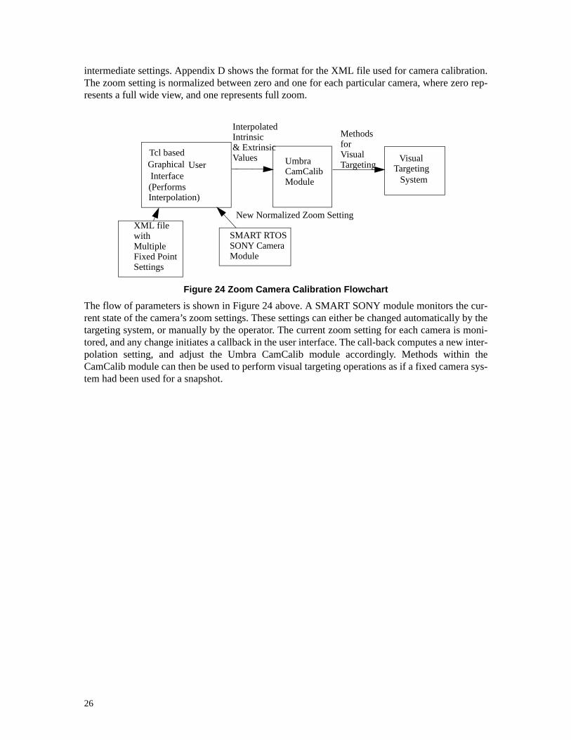
intermediate settings. Appendix D shows the format for the XML file used for camera calibration.The zoom setting is normalized between zero and one for each particular camera, where zero rep-resents a full wide view, and one represents full zoom.
Figure 24 Zoom Camera Calibration FlowchartThe flow of parameters is shown in Figure 24 above. A SMART SONY module monitors the cur-rent state of the camera’s zoom settings. These settings can either be changed automatically by thetargeting system, or manually by the operator. The current zoom setting for each camera is moni-tored, and any change initiates a callback in the user interface. The call-back computes a new inter-polation setting, and adjust the Umbra CamCalib module accordingly. Methods within theCamCalib module can then be used to perform visual targeting operations as if a fixed camera sys-tem had been used for a snapshot.
Tcl basedGraphical User Interface
UmbraCamCalibModule
SMART RTOSSONY CameraModule
New Normalized Zoom Setting XML filewith Multiple Fixed Point Settings
(PerformsInterpolation)
InterpolatedIntrinsic& ExtrinsicValues
MethodsforVisualTargeting
VisualTargeting
System
26
6.0 Conclusions
In this LDRD we have explored the use of visual imagery for automating operations with mobilemanipulator systems used in emergency response.During the course of this LDRD we demonstrated the use of statistical pressure snakes for auto-mating tool pickups. The experiment consisted of a 6-degree-of-freedom (DOF) robot system witha wrist mounted camera. Special made tool pickups were designed that contained a uniquely col-ored a rectangular block attached to a robot tool. The robot was able to automatically approach,align itself and grab the robot tool by responding to information gleaned from the snake. Toolalignment variations in 4-DOF, (3 translation, and z-axis rotation) could be readily accommodatedwith this approach. The snake algorithms proved to be robust in the unstructured lighting condi-tions typically seen by emergency response manipulators.We also further developed visual targeting and active sketch technologies. By providing simpleobject primitives to the operator, and a derived list of tasks based on the primitives, we’ve devel-oped an interface which is fast, intuitive and powerful for a wide range of activities, such as grasp-ing objects, opening doors and scanning surfaces.We demonstrated that live video imagery could be utilized by the robotic operators within a 3-Dmodelling environment. Operators are often plagued with a tunnel vision phenomena, where theyhave the video feed, but lose the context of the video. By embedding the video within a 3-D worldmodel, this problem is addressed. The operator is able to freely move from video perspective tooverview perspective and back. The 3-D world serves as a working environment to embed newinformation as it is received.Finally, several advancements in camera calibration have been made. An interactive, graphical toolfor bench top calibration of intrinsic and extrinsic camera parameters has been developed. Arobust algorithm for non-perspective n-point pose estimation has been developed, and is beingincorporated into an interactive pose estimation tool. New zoom camera systems have been inves-tigated, and a working continuously variable calibration model has been developed which is com-patible with existing targeting systems.
27
7.0 References
[1] D. Perrin and C. Smith, “Rethinking classical internal forces for active contour models,” Proceedings of the IEEE International Conference on Computer Vision and Pattern Recognition, 2001.
[2] HP Schaub & C.E. Smith, “Color Snakes for Dynamic Lighting Conditions on Mobile Manipulation Platforms”, Proceedings IEEE/RSJ International Conference on Intelligent Robots and Systems, Las Vegas, Oct. 2003
[3] H. Schaub, “Statistical Pressure Snakes based on Color Images”, SAND-Report 2004-1867.
[4] H. Schaub, “Visual Servoing Using Statistical Pressure Snakes,” SAND-Report 2004-1868.
[5] H. Schaub, “Extracting Primary Features of a Statistical Pressure Snake”, SAND-Report 2004 1869.
[6] H. Schaub, “Reading Color Barcodes using Visual Snakes,” SAND-Report 2004 1870.
[7] H. Schaub, “Matching a Statistical Pressure Snake to a Four-Sided Polygon and Estimating the Polygon Corners,” SAND 2004 1871.
[8]R. J. Anderson, “Modular Architecture for Robotics and Teleoperation”, U.S. Patent No. 5581666. Dec. 3, 1996.
[9]R. J. Anderson, “SMART: A Modular Control Architecture for Telerobotics,” IEEE Robotics and Automation Society Magazine, pp. 10-18, Sept. 95.
[10]R. J. Anderson, “SMART: A Modular Control Architecture for Telerobotics,” IEEE Robotics and Automation Society Magazine, pp. 10-18, Sept. 95.
[11]E. J. Gottlieb, M. McDonald and et. all, “The Umbra Simulation Framework as Applied to Building HLA Federates,” Proceedings of the 2002 Winter Simulation Conference, pp. 981-989
[12]E. J. Gottlieb, M. J. McDonald, and F.J. Oppel, “The Umbra High Level Architecture Interface,” Sandia Technical Report SAND2002-0675.
[13]G., DeSouza and A. Kark, “Vision for Mobile Robot Navigation: A Survey,” IEEE Transactions on Pattern Analysis and Machine Intelligence, vol. 24. no. 2, pp 237-267, 2002.
[14] R. W. Harrigan and P. C. Bennett, “Making Remote Manipulators Easy to Use”, Unmanned Ground Vehicle Technology III (SPIE International) Symposium, 2001 Orlando FL.
[15] M. McDonald, R.J. Anderson and S. Gladwell, “Active Sketch A New Human Interface”, Patent Application, filed Dec. 17, 2002. (Status pending)
[16] R. Y. Tsai, “A Versatile Camera Calibration Technique for 3D Machine Vision,” IEEE J. Robotics & Automation, RA-3, No. 4, August 1987, pp. 323-344.
[17] J. Weng, P. Cohen and M. Herniou, “Camera Calibration and Distortion Models and Accuracy Evaluation,” IEEE Transactions on Pattern Analysis & Machine Intelligence, vol. 14, no. 10, Oct. 1992., pp. 965-980.
[18] Z. Zhang, “A Flexible New Technique for Camera Calibration,” IEEE Transaction on Pattern Analysis and Machine Intelligence, Vol. 22, No. 11, Nov. 2000, pp. 1330-1334.
[19] http://developer.intel.com, “Open Source Computer Vision Library: Reference Manual,” Order Number: 123456-001.
[20] C-S Chen and W.Y. Chang, “Pose Estimation for Generalized Imaging Device via Solving Non-Perspective N Point Problem,” Proceedings of the 2002 IEEE International Conference on Robotics & Automation, Washington, DC, May 2002. pp. 2931-2937.
28

Appendix A: Camera Calibration Terminology
Camera calibration is the process of determining the relationship between 2-D image points and 3-D world points. There is a large body of work developing camera calibration approaches and techniques. This section defines the notation and provides an overview of the algorithms employed for computing the camera calibration (as used by the camCalib Umbra module).
A 3-D point, xi, is represented in homogenous coordinates as
(4)
and a 2-D image point (ui, vi) is represented in homogenous coordinates as
(5)
where
(6)
The mapping between the two frames utilizes the camera calibration matrix.
(7)
and is given by
(8)
It is possible to solve for the elements of C for a given camera by recording the u, v coordinates ofvarious points that are defined in x, y, z coordinates. Following the approach in [1], but applyingthe notation used here
xi
xi
yi
zi
1
=
ui
Ui
Vi
ti
=
uiUiti-----=
viViti-----=
Cc11 c12 c13 c14
c21 c22 c23 c24
c31 c32 c33 c34
c1
c2
c3
= =
ui Cxi=
29

(9)
Expanding the inner products and utilizing equation 6 gives the following mapping (where c34 hasbeen set to one since the scaling on the matrix is arbitrary).
(10)
This represents a linear equation in the unknown parameters cii which is valid for pair of xyz anduv parameters. By applying this equation to n sample pairs (x1 through xn) a overdetermined sys-tem of equations can result, as shown below:
(11)
Ui
Vi
ti
c11 c12 c13 c14
c21 c22 c23 c24
c31 c32 c33 c34
xi
yi
zi
1
=
xi yi zi 1 0 0 0 0 uixi– uiyi– uizi–0 0 0 0 xi yi zi 1 vixi– viyi– vizi–
c11
c12
c13
c14
c21
c22
c23
c24
c31
c32
c33
ui
vi
=
x1 y1 z1 1 0 0 0 0 u1x1– u1y1– u1z1–0 0 0 0 x1 y1 z1 1 v1x1– v1y1– v1z1– .
xn yn zn 1 0 0 0 0 unxn– unyn– unzn–0 0 0 0 xn yn zn 1 vnxn– vnyn– vnzn–
c11
c12
c13
c14
c21
c22
c23
c24
c31
c32
c33
u1
v1
.un
vn
=
30
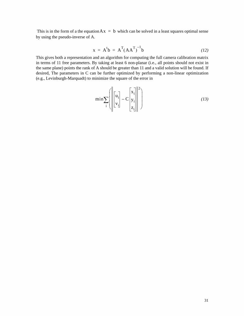
This is in the form of a the equation which can be solved in a least squares optimal senseby using the pseudo-inverse of A.
(12)
This gives both a representation and an algorithm for computing the full camera calibration matrixin terms of 11 free parameters. By taking at least 6 non-planar (i.e., all points should not exist inthe same plane) points the rank of A should be greater than 11 and a valid solution will be found. Ifdesired, The parameters in C can be further optimized by performing a non-linear optimization(e.g., Levinburgh-Marquadt) to minimize the square of the error in
(13)
Ax b=
x Atb AT AAT( )1–b= =
minui
vi
Cxi
yi
zi
–
2
⎝ ⎠⎜ ⎟⎜ ⎟⎜ ⎟⎛ ⎞
i∑
31
Appendix B: Using the Extrinsic/Intrinsic Reference Model
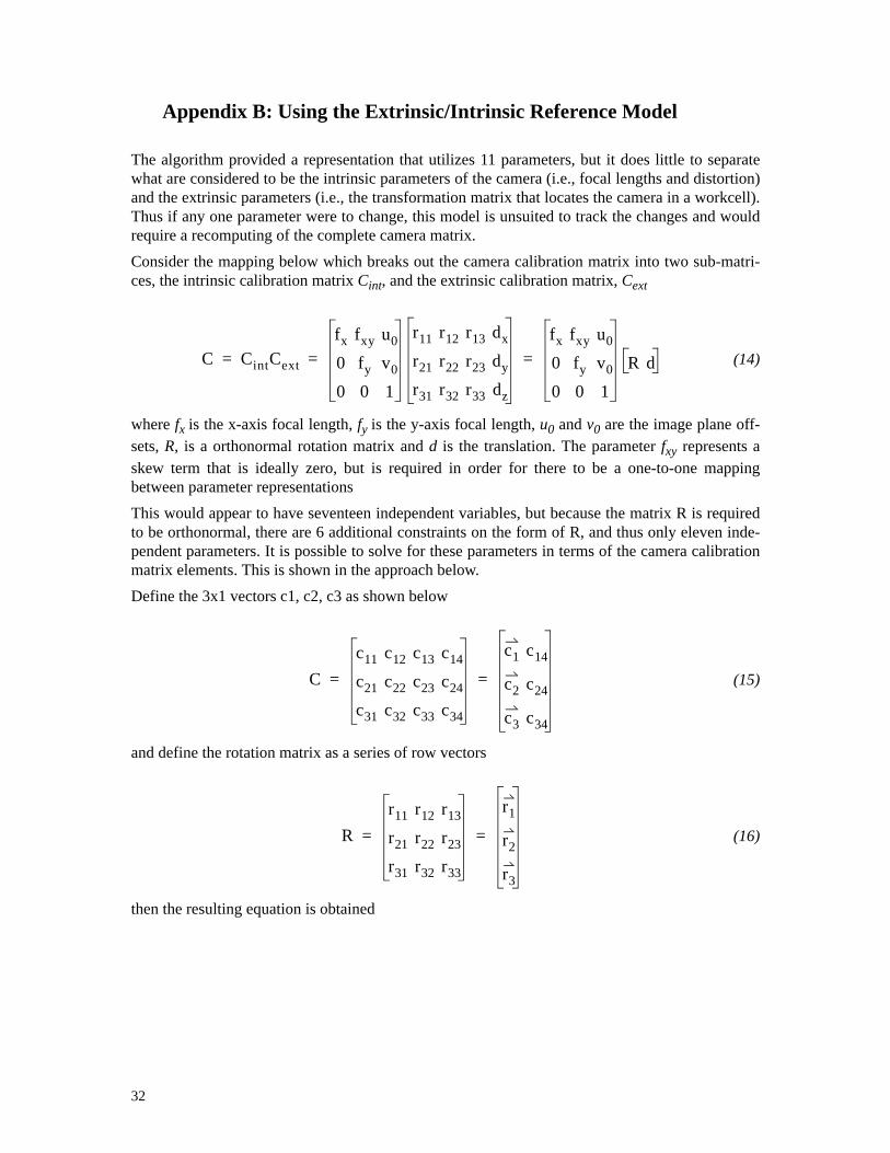
The algorithm provided a representation that utilizes 11 parameters, but it does little to separatewhat are considered to be the intrinsic parameters of the camera (i.e., focal lengths and distortion)and the extrinsic parameters (i.e., the transformation matrix that locates the camera in a workcell).Thus if any one parameter were to change, this model is unsuited to track the changes and wouldrequire a recomputing of the complete camera matrix.Consider the mapping below which breaks out the camera calibration matrix into two sub-matri-ces, the intrinsic calibration matrix Cint, and the extrinsic calibration matrix, Cext
(14)
where fx is the x-axis focal length, fy is the y-axis focal length, u0 and v0 are the image plane off-sets, R, is a orthonormal rotation matrix and d is the translation. The parameter fxy represents askew term that is ideally zero, but is required in order for there to be a one-to-one mappingbetween parameter representationsThis would appear to have seventeen independent variables, but because the matrix R is requiredto be orthonormal, there are 6 additional constraints on the form of R, and thus only eleven inde-pendent parameters. It is possible to solve for these parameters in terms of the camera calibrationmatrix elements. This is shown in the approach below.Define the 3x1 vectors c1, c2, c3 as shown below
(15)
and define the rotation matrix as a series of row vectors
(16)
then the resulting equation is obtained
C CintCext
fx fxy u0
0 fy v0
0 0 1
r11 r12 r13 dx
r21 r22 r23 dy
r31 r32 r33 dz
fx fxy u0
0 fy v0
0 0 1R d= = =
Cc11 c12 c13 c14
c21 c22 c23 c24
c31 c32 c33 c34
c1 c14
c2 c24
c3 c34
= =
Rr11 r12 r13
r21 r22 r23
r31 r32 r33
r1
r2
r3
= =
32

(17)
From the bottom row of this equation the following equalities:
(18)
Because the matrix C can be arbitrarily scaled and the vector r3 must have a unit norm, it is clearthe matrix must first be normalized accordingly.
(19)
In this case the term c34 is no longer unit valued, but directly gives the value for dz.
From the second row of Eq. 17,
(20)
Multiplying both sides by r3 and taking advantage of the orthonormal requirement on R gives
(21)
Once v0 is known then the focal length fy and rotation vector r3 can be retrieved by utilizing theunit value condition on r3.
(22)
(23)
The top row of Eq. 17 gives us
(24)
Using the same orthonormal constraints on R gives us
(25)
(26)
C
c1 c14
c2 c24
c3 c34
fx fxy u0
0 fy v0
0 0 1
r11 r12 r13 dx
r21 r22 r23 dy
r31 r32 r33 dz
fx fxy u0
0 fy v0
0 0 1
r1 dx
r2 dy
r3 dz
= = =
dz c34=
c3 r3=
C
C C
c312 c32
2 c332+ +
---------------------------------------=
c2 fyr2 v0r3+=
r3T
c2 r3T
fyr2 v0r3+( ) v0= =
fy c2 v0r3–=
r2c2 v0r3–
fy---------------------=
c1 fxr1 fxyr2 u0r3+ +=
u0 r3T
c1=
fxy r2T
c1=
33
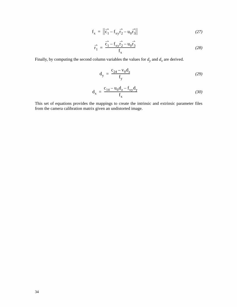
(27)
(28)
Finally, by computing the second column variables the values for dy and dx are derived.
(29)
(30)
This set of equations provides the mappings to create the intrinsic and extrinsic parameter filesfrom the camera calibration matrix given an undistorted image.
fx c1 fxyr2– u0r3–=
r1c1 fxyr2– u0r3–
fx---------------------------------------=
dyc24 v0dz–
fy------------------------=
dxc14 u0dz– fxydy–
fx-------------------------------------------=
34

Appendix C: Solving the non-Perspective n-Point problem
For a series of XYZ points attached to an object frame, viewed from a imaging device (i.e., PTUcamera), the imaging equation relating the image coordinates to XYZ points is given by
(31)
Typically may vary for each point taken but is well known, is known and fixed, isconsidered known (but may vary based on zoom settings), and the goal of the pose estimation is todetermine either or accurately, assuming every other transform is known for the givenview, and that the value for either of these transforms is fixed for multiple measurements.Without loss of generality equation 31 simplifies to
(32)
where depending on which transforms are known a priori.
or (33)
(34)
Defining the transform
(35)
it follows that
Ui
Vi
ti
Cint I3
000
TextTkinTdevTobj1–
xi
yi
zi
1
=
Tkin Text Cint
Tdev Tobj
Ui
Vi
ti
Cint I3
000
TATest
xi
yi
zi
1
=
xi
yi
zi
1
Tobj1–
xi
yi
zi
1
= TA TextTkin= Test Tdev=
xi
yi
zi
1
xi
yi
zi
1
= TA TextTkinTdev= Test Tobj1–=
TARA dA
03 1⁄ 1=
35

(36)
Representing the estimated transform using a first order approximation
(37)
where is the skew-symmetry operator, is the initial rotation estimate, is
the initial distance estimate, is the angular correction, and is the position correction.
(38)
substituting again gives
(39)
where
Ui
Vi
ti
Cint I3
000
TATest
xi
yi
zi
1
Cint RA dA Test
xi
yi
zi
1
= =
TestRest dest
03 1⁄ 1R0 X ∆θ( )R0+ d0 ∆d+
03 1⁄ 1= =
X( ) R0 eX θ0( )
= d0
∆θ ∆d
Ui
Vi
ti
Cint RA dAR0 X ∆θ( )R0+ d0 ∆d+
03 1⁄ 1
xi
yi
zi
1
=
CintRAR0
xi
yi
zi
CintRAX ∆θ( )R0
xi
yi
zi
CintRAd0 CintdA CintRA∆d+ + + +=
CintRAR0
xi
yi
zi
CintRAd0 CintdA+ CintRAX R0
xi
yi
zi⎝ ⎠⎜ ⎟⎜ ⎟⎜ ⎟⎛ ⎞
∆θ– CintRA∆d+ +=
uiti
viti
ti
λ10
λ20
λ30
λ11 λ12 λ13 λ14 λ15 λ16
λ21 λ22 λ23 λ24 λ25 λ26
λ31 λ32 λ33 λ34 λ35 λ36
∆θ∆d
+λ10
λ20
λ30
λ1
λ2
λ3
Φ+= =
36

(40)
(41)
(42)
Finally, solving for and substituting
(43)
(44)
(45)
This is of the linear equation form
A least squares fit is then obtained by taking multiple points and fitting the data.
(46)
(47)
λ10
λ20
λ30
CintRAR0
xi
yi
zi
CintRAd0 CintdA++=
Cint RA R0
xi
yi
zi
d0+
⎝ ⎠⎜ ⎟⎜ ⎟⎜ ⎟⎛ ⎞
dA+
⎝ ⎠⎜ ⎟⎜ ⎟⎜ ⎟⎛ ⎞
=
λ11 λ12 λ13
λ21 λ22 λ23
λ31 λ32 λ33
C– intRAX R0
xi
yi
zi⎝ ⎠⎜ ⎟⎜ ⎟⎜ ⎟⎛ ⎞
=
λ14 λ15 λ16
λ24 λ25 λ26
λ34 λ35 λ36
CintRA=
Φ
ti λ30 λ3Φ+=
ui λ30 λ3Φ+( )
vi λ30 λ3Φ+( )
λ10
λ20
λ1
λ2
Φ+=
λ30ui λ10–
λ30vi λ20–λ1 uiλ3–
λ2 viλ3–Φ=
bi AiΦ=
b1
b2
…bn
A1
A2
…An
Φ b AΦ= = =
Φ A⊥b ATA( )1–ATb= =
37

In summary, the algorithm is as follows.
First, compute the least squares equation 47 to solve for where
(48)
Second, compute a new rotation R matrix
(49)
Using the axis angle representation,
(50)
the new rotation matrix can be written as
(51)
Φ ∆θ∆d
=
Aiλ1 uiλ3–
λ2 viλ3–bi,
λ03ui λ01–
λ03vi λ02–= =
θ0 k 1+( ) θ0 k( ) ∆θ+=
R0 k 1+( ) eX θ0 ∆θ+( )
=
d0 k 1+( ) d0 k( ) ∆d+=
φ θ0=
kθ0θ0
----------=
R φ( )I3cos 1 φ( )cos–( )kkT
φ( )X k( )sin+ +=
38
Appendix D: XML Format for Zoom Camera Calibration
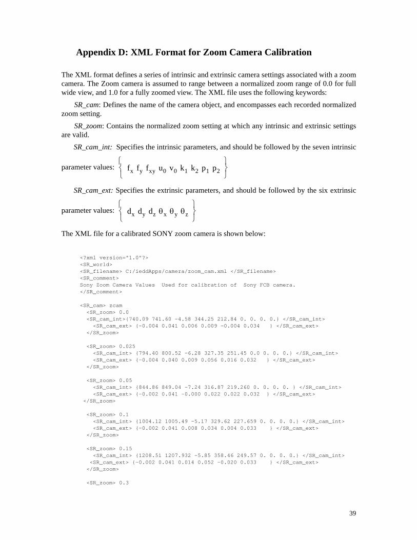
The XML format defines a series of intrinsic and extrinsic camera settings associated with a zoomcamera. The Zoom camera is assumed to range between a normalized zoom range of 0.0 for fullwide view, and 1.0 for a fully zoomed view. The XML file uses the following keywords:
SR_cam: Defines the name of the camera object, and encompasses each recorded normalizedzoom setting.
SR_zoom: Contains the normalized zoom setting at which any intrinsic and extrinsic settingsare valid.
SR_cam_int: Specifies the intrinsic parameters, and should be followed by the seven intrinsic
parameter values:
SR_cam_ext: Specifies the extrinsic parameters, and should be followed by the six extrinsic
parameter values:
The XML file for a calibrated SONY zoom camera is shown below:
<?xml version="1.0"?><SR_world><SR_filename> C:/ieddApps/camera/zoom_cam.xml </SR_filename><SR_comment>Sony Zoom Camera Values Used for calibration of Sony FCB camera.</SR_comment>
<SR_cam> zcam <SR_zoom> 0.0 <SR_cam_int>{740.09 741.60 -4.58 344.25 212.84 0. 0. 0. 0.} </SR_cam_int> <SR_cam_ext> {-0.004 0.041 0.006 0.009 -0.004 0.034 } </SR_cam_ext> </SR_zoom>
<SR_zoom> 0.025 <SR_cam_int> {794.40 800.52 -6.28 327.35 251.45 0.0 0. 0. 0.} </SR_cam_int> <SR_cam_ext> {-0.004 0.040 0.009 0.056 0.016 0.032 } </SR_cam_ext> </SR_zoom>
<SR_zoom> 0.05 <SR_cam_int> {844.86 849.04 -7.24 316.87 219.260 0. 0. 0. 0. } </SR_cam_int> <SR_cam_ext> {-0.002 0.041 -0.000 0.022 0.022 0.032 } </SR_cam_ext> </SR_zoom>
<SR_zoom> 0.1 <SR_cam_int> {1004.12 1005.49 -5.17 329.62 227.659 0. 0. 0. 0.} </SR_cam_int> <SR_cam_ext> {-0.002 0.041 0.008 0.034 0.004 0.033 } </SR_cam_ext> </SR_zoom>
<SR_zoom> 0.15 <SR_cam_int> {1208.51 1207.932 -5.85 358.46 249.57 0. 0. 0. 0.} </SR_cam_int> <SR_cam_ext> {-0.002 0.041 0.014 0.052 -0.020 0.033 } </SR_cam_ext> </SR_zoom>
<SR_zoom> 0.3
fx fy fxy u0 v0 k1 k2 p1 p2⎩ ⎭⎨ ⎬⎧ ⎫
dx dy dz θx θy θz⎩ ⎭⎨ ⎬⎧ ⎫
39

<SR_cam_int> {2314.0 2319.32 -15.74 321.77 139.95 0. 0. 0. 0.} </SR_cam_int> <SR_cam_ext> {-0.002 0.042 0.019 0.001 0.003 0.034 } </SR_cam_ext> </SR_zoom>
<SR_zoom> 0.4 <SR_cam_int> {3500.0 3500.0 0.0 320.0 240.0 0.0 0.0 0.0 0.0} </SR_cam_int> <SR_cam_ext> {-0.001 0.041 0.021 0.078 0.051 0.032 } </SR_cam_ext> </SR_zoom>
<SR_zoom> 1.0 <SR_cam_int> {29600.0 29600.0 0.0 320.0 240.0 0.0 0.0 0.0 0.0} </SR_cam_int> <SR_cam_ext> {-0.001 0.041 0.021 0.022 0.022 0.032 } </SR_cam_ext> </SR_zoom></SR_cam></SR_world>
40
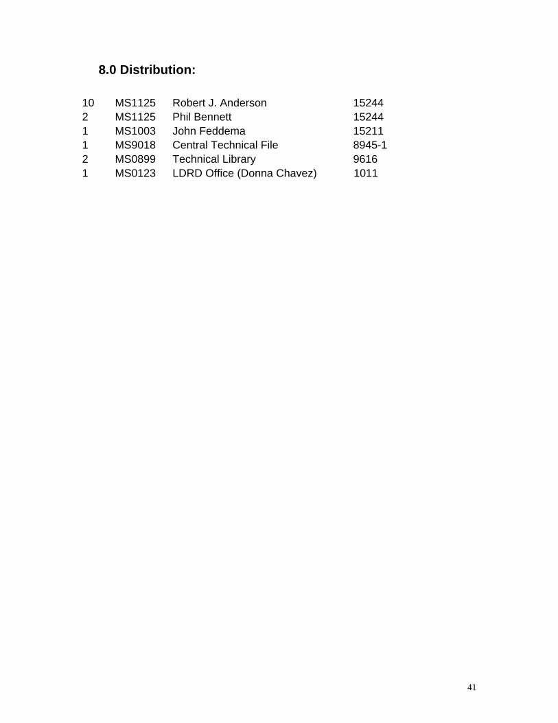
8.0 Distribution:
10 MS1125 Robert J. Anderson 152442 MS1125 Phil Bennett 152441 MS1003 John Feddema 152111 MS9018 Central Technical File 8945-12 MS0899 Technical Library 96161 MS0123 LDRD Office (Donna Chavez) 1011
41