EE225E/BIOE265 Spring 2012 Miki LustigPrinciples of MRI

Assignment 4

Due Feb 19, 2012

1. Finish reading Nishimura Ch.4 and Ch. 5.

2. Graphical interpretation of k-space. Consider the following (demodulated) signal which isobtained while scanning an unknown object with an unknown gradient waveform. Three candidategradient waveforms are shown below the received signal. For each of the three gradient waveforms,explain if it could have been the actual gradient used to acquire this MRI signal.

Bioeng 265 Prof. Steve Conolly

Homework #3 Due: Friday, 20 Feb, 2009

1. Nishimura 4.4

2. Assume at t=0 a constant gradient is on with G=10 mT/m. Let the object be

two delta functions at ! x0.(a) Derive the demodulated MRI signal with a constant gradient. (b) Explain from the received signal which half of k-space is available.(c) How could you recover the other half of k-space given a priori knowledge that the object is Real Valued? Explain.

3. Graphical interpretation of k-space.Consider the following (demodulated) signal which is obtained while scanning an unknown object with an unknown gradient waveform. Three candidate gradient waveforms are shown below the received signal. For each of the three gradient waveforms, explain if it could have been the actual gradient used to acquire this MRI signal.

S(t)

time

Ga(t)

Gb(t)

Gc(t)

1

2

1.

2

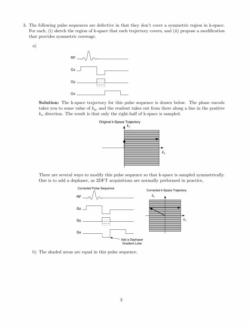
3. The following pulse sequences are defective in that they don’t cover a symmetric region in k-space.For each, (i) sketch the region of k-space that each trajectory covers, and (ii) propose a modificationthat provides symmetric coverage.

a)

Gx

Gy

Gz

RF

Solution: The k-space trajectory for this pulse sequence is drawn below. The phase encodetakes you to some value of ky, and the readout takes out from there along a line in the positivekx direction. The result is that only the right-half of k-space is sampled.

kx

kyOriginal k-Space Trajectory

There are several ways to modify this pulse sequence so that k-space is sampled symmetrically.One is to add a dephaser, as 2DFT acquisitions are normally performed in practice,

Gx

Gy

Gz

RF

kx

ky

Add a DephaserGradient Lobe

Corrected k-Space TrajectoryCorrected Pulse Sequence

b) The shaded areas are equal in this pulse sequence.

3

Gx

Gy

Gz

RF

Solution: The k-space trajectory for this pulse sequence is drawn below. They gradient goesto some −ky.max, and then goes to ky,max at a constant rate. While it is going in the positivedirection, Gx is oscillating sinusoidally. The kx position is then proportional to the integral of asine. However, this is never negative. The result is the k-space trajectory plotted below on theleft;

kx

kyOriginal k-Space Trajectory Corrected k-Space Trajectory

kx

ky

Acq 1Acq 2

Again, there are several ways to fix this trajectory. One option is to add a dephaser, as in (a).Another alternative is to add a second acquistion with the sign of Gx inverted. The result is thek-space trajectory plotted above on the right. The pulse sequence for this trajectory is plottedbelow, with the solid line corresponding to the Gx gradient for the first acquisition, and thedashed line corresponding to the second acquisition.

Corrected Pulse Sequence

Gx

Gy

Gz

RF

This approach was advocated by the Mansfield group when they were developing EPI, whichthey called BEST (I can’t reconstruct what this was an acronym for). This version of BESTwas called MBEST, for Mosaic BEST.

4

c) The amplitude of the readout gradients are incremented together, so that for the ith acquisition

the gradient amplititudes are Gx = Gy = Gmax(iN

).

Gx

Gy

Gz

RF

Solution: The k-space trajectory in this case is a sequence of nested diamonds, as shown belowon the left:

kx

kyOriginal k-Space Trajectory

kx

kyCorrect k-Space Trajectory

Gx,Gy

−Gx,−Gy

−Gy,Gx

Gy,−Gx

Again we could fix this trajectory by adding a dephaser as in (a), and shift the entire patternto the left.

Another solution is to repeat the acquisition so as to tile k-space. One solution is to play Gx andGy waveforms as originally indicated for the first acquisition, and −Gx and −Gy waveforms forthe second. Then two more acquisitions with the gradient axes reversed complete the pattern.These are −Gy, G, x for the third, and Gy,−Gx for the fourth. The k-space coverage that thisproduces is shown on the right above.

Aside from the sign changes, and swapping the gradients between channels, the pulse sequencelooks the same.

5

4. The following pulse sequence is performed repeatedly, with varying values of θ.

Gx

Gy

Gz

RF

G sinθ

G cosθ

We would like the pulse sequence to cover a symmetric region of k-space.

a) What range should the range of the angle θ be? Find the minimum and maximum values ofθ, and don’t worry about how finely θ is sampled. Sketch the resulting k-space trajectory, andk-space coverage.

Solution: The k-space coverage of this pulse sequence is shown below:

kx

ky

Each acquisition starts at the k-space origin and goes directly out on a radius. The range of θshould go from 0 to 2π to completely cover the disk.

b) Compute the readout gradient duration if the maximum gradient is 4 G/cm, and we want 0.5mm resolution.

Solution:

If we want 0.5 mm = 0.05 cm resolution, we need a k-space extent of

Wkx =1

δx=

1

0.05= 20 cycles/cm.

Each acquisition covers half of this, starting from 0, and going out to a radius of 10 cycles/cm.If the amplitude of the readout gradient is G, and the duration τ , the radius in k-space that is

6

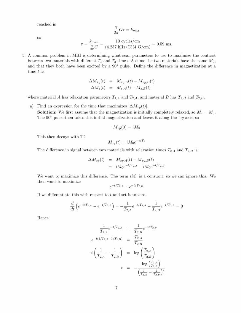
reached isγ

2πGτ = kmax

so

τ =kmaxγ2πG

=10 cycles/cm

(4.257 kHz/G)(4 G/cm)= 0.59 ms.

5. A common problem in MRI is determining what scan parameters to use to maximize the contrastbetween two materials with different T1 and T2 times. Assume the two materials have the same M0,and that they both have been excited by a 90◦ pulse. Define the difference in magnetization at atime t as

∆Mxy(t) = Mxy,A(t)−Mxy,B(t)

∆Mz(t) = Mz,A(t)−Mz,B(t)

where material A has relaxation parameters T1,A and T2,A, and material B has T1,B and T2,B.

a) Find an expression for the time that maximizes |∆Mxy(t)|.Solution: We first assume that the magnetization is initially completely relaxed, so Mz = M0.The 90◦ pulse then takes this initial magnetization and leaves it along the +y axis, so

Mxy(0) = iM0

This then decays with T2Mxy(t) = iM0e

−t/T2

The difference in signal between two materials with relaxation times T2,A and T2,B is

∆Mxy(t) = Mxy,A(t)−Mxy,B(t)

= iM0e−t/T2,A − iM0e

−t/T2,B

We want to maximize this difference. The term iM0 is a constant, so we can ignore this. Wethen want to maximize

e−t/T2,A − e−t/T2,B

If we differentiate this with respect to t and set it to zero,

d

dt

(e−t/T2,A − e−t/T2,B

)= − 1

T2,Ae−t/T2,A +

1

T2,Be−t/T2,B = 0

Hence

1

T2,Ae−t/T2,A =

1

T2,Be−t/T2,B

e−t(1/T2,A−1/T2,B) =T2,AT2,B

−t(

1

T2,A− 1

T2,B

)= log

(T2,AT2,B

)

t = −log

(T2,AT2,B

)(

1T2,A− 1

T2,B

))

7

b) Find an expression for the time that maximizes |∆Mz(t)|.Solution: The z magnetization after the 90◦ pulse is zero, so that

Mz(t) = (1− e−t/T1)M0

The difference in Mz for two materials with relaxation times T1,A and T1,B is then

∆Mz(t) = Mz,A(t)−Mz,B(t)

= (1− e−t/T1,A)M0 − (1− e−t/T1,B )M0

= (e−t/T1,B − e−t/T1,A)M0

We want to maximizee−t/T1,B − e−t/T1,A

This is the same problem as in part (a), with the two materials interchanged. Since we shouldget the same answer either way we label the two, the answer has the same form as in (a)

t = −log

(T1,AT1,B

)(

1T1,A− 1

T1,B

)).

8

6. This question is taken from midterm Sp ’10TRUE or FALSE

For each of the following statements, identify weather it is True or False. To get a score you needalso to provide a brief explanation for either case.

a) For sequences with short time-repetitions (TR), doubling the main field (B0) always resultsin double the SNR. Solution: In general the magnetization increased linearly with the fieldstrength. So, doubling the field gives double the signal. So, at 3T we should expect twice theSNR as in 1.5T. However, the question specifically asks about short time-repetitions. The signalwith short time repetitions depends heavily on T1 recovery, and T1 becomes longer with magneticfield strength. Longer T1 means longer time to recover the magnetization after excitation andtherefore will exhibit lower signal for short time repetitions. So, we should expect less than afactor of 2 increase in SNR.

FALSE: Magnetization is proportional to B0. However, T1 increases with B0. In short TRsequences, signal decreases as T1 increases.

b) The FID from n Conollyum nuclei ( γ2π = 4 kHz/G) at 1.5T is identical to the FID from

n Pinesume nuclei ( γ2π = 1 kHz/G) at 6T. Solution: Both the Conollyum nuclei and the

Pinesume nuclei will resonate at 60MHz because the resonance frequency is γ2πB0. However,

the magnetization ( see Nishimura book) is proportional to γ2B0, so the signal from Conollyumwill be stronger.

FALSE: The frequency will be the same, but the magnitude is proportional to γ2B0.

c) (short T2, long T1) species are easier to image in vivo than (long T2, short T1) species. Solution:In in vivo imaging we would like to image as fast as we can and get the most SNR that we can.Long T2 allows longer readout time after each excitation because the signal persists for a longertime. Short T1 allows fast repetition of excitations because the magnetization recovers very fast.Therefore it is easy to image (long T2, short T1) species and it is much harder to do so in invivo conditions in the case of (short T2, long T1).

FALSE: short T2 → short readout time, long T1 → long repetition timeboth→ slow acquisition and low SNR efficiency, which are inappropriate for in vivo imaging

9

7. Matlab Excercise: Bloch simulation and spin visualization In this exercise you will simulateand visualize the behavior of a spin in the presence of magnetic fields. For this purpose we will use aMatlab implementation of a Bloch simulator that was written by Prof. Brian Hargreaves of StanfordRadiology.

• The Bloch simulator. Download the Bloch simulator files : bloch.m and bloch.c from the classwebsite. The file bloch.c is a mex file implementation that is used to accelerate the computationof the solution for the Bloch equation. You will first need to compile the executable for yourparticular computer architecture. In your Matlab command window type:

>> mex bloch.c

Ignore any warnings from the compilation. If you encounter problems compiling the the mexfile you can try downloading the executable for your platform from the class website

Read the help for the function bloch by typing

>> help bloch

Here’s a simple example showing T2 decay and T1 recovery:

>> dt = 4e-6; % 4 us sampling rate

>> rf_90 = 90/360/(4257*dt);

>> % impulse RF pulse

>> b1 = [rf_90;zeros(300e-3/dt,1)];

>> g = b1*0; % no gradient

% the spin is on-resonance

>> df = 0;

>> % the spin at iso-center

>> dp = 0;

>> t1 = 100e-3;

>> t2 = 50e-3;

>> % start at Mz

>> mx_0 = 0;

>> my_0 = 0;

>> mz_0 = 1;

>> % Simulate

>> [mx,my,mz] = bloch(b1,g,dt,t1,t2,df,dp,2,mx_0,my_0, mz_0);

>> %plot

>> time = [1:length(mx)]*dt;

>> figure, plot(time,mx,time,my,time,mz); legend(’Mx’,’My’,’Mz’);

This is the plot you should get:

10

• Design an RF waveform, sampled at 4µs with maximum |B1| < 0.16G that produces a 90◦

rotation. What is the length of the pulse and what is the amplitude?Solution:There are many right answers here, since there is freedom to chose any combination of B1 andpulse duration. The number of samples for B1 = 0.16 is N = 0.25/(γ B1max dt) = 91.76. Weround upwards and adjust the RF to B1 = 0.1596G. The duration is 92 ∗ 4 = 368µs.

• Design a gradient waveform with |G| < 4G/cm and |dGdt | < 15000G/cm/s that produces arotation of 2 cycles for spins located at 0.2cm off iso-center. You can use the function you wrotein the previous homework! What is the length of the pulse?Solution:2 cycles per 0.2cm means that we need a gradient area that achieves 10 cycles/cm, which is10 · 2π/γ. Using the gradient design function from the previous homework we get a trapezoidgradient with maximum amplitude of 4G/cm and duration 0.852ms.

• Perform a simulation of a period of t = 100ms, in which first the RF is applied, followed by thegradient and then no-filed is applied. Simulate a spin at 0.2cm from iso-center with T1 =30e-3and T2 =15e-3. Plot Mx,My, and Mz as a function of time.Solution:

11

• Visualization: Download the files: visualizeMagn.m, arrow3D.m, rotatePoints.m from theclass website. The function visualizeMagn renders an animation of the spin and the fields. Thefirst argument is a vector of the applied B1 field in Gauss. The second argument is the vector ofthe effective B0 field. In this case it will be the gradient field times the position of the spin. Thethird argument is an array of the magnetization vector vs time. It should be [N x 3] representingMx My and Mz at each time point. The last argument is the acceleration factor of the rendering(you should use at least 10 if you are impatient).

This is the plot you should get for the previous example by running:

>> visualizeMagn(zeros(size(mx)), zeros(size(mx)), [mx,my,mz],100);

Render the simulation and submit the plot of the final result.Solution:The spin is excited to the transverse plane, does 2 rotations and then relaxes back to equilibrium.

• Now, simulate and visualize the sequence 90RF, Gradient, -90RF for a spin at: 0cm, 0.025cm,0.05cm, 0.075cm and 0.1cm. Use the same gradient you used previously and T1 = 1000 andT2 = 1000.What can you say about the distribution of Mz in space after this sequence?Solution:The result we get is 1,0,-1,0,1 for discrete locations. In the continuum we get that the distributionof the longitudal magnetization is Mz = cos(2π10x)

12

The Matlab code is:

gamma = 4257;

dt = 4e-6;

B1max=0.16;

Smax = 15000;

Gmax = 4;

% find the number of samples and b1

N = ceil(0.25/(gamma*B1max*dt));

b1 = ones(N,1)*0.25/(gamma*N*dt);

% find gradient 2cycles/0.2cm -> 10cycles/cm

x = 0.2;

area = 2/0.2/gamma

g = minTimeGradientArea(area, Gmax, Smax, dt);

B1 = zeros(0.1/dt,1);

G = B1;

B1(1:length(b1)) = b1;

G(length(b1)+1:length(b1)+length(g)) = g;

[mx,my,mz] = bloch(B1,G,dt,30e-3,15e-3,0,x,2,0,0,1);

t = [1:length(mx)]*dt;

rfg = 1:(length(b1)+length(g));

figure,

subplot(211), plot(t(rfg),mx(rfg),t(rfg),my(rfg),t(rfg),mz(rfg));

legend(’mx’,’my’,’mz’); title(’RF and gradient’)

subplot(212),

plot(t,mx,t,my,t,mz);

legend(’mx’,’my’,’mz’); title(’RF, gradient and relaxation’)

visualizeMagn(B1, G*x, [mx,my,mz],10);

%%%%%%%%%%%%%%%% Part II %%%%%%%%%%%%%%%%%%%%

B1 = [b1;g*0;-b1];

G = [0*b1;g;0*b1];

for x=[0,0.025, 0.05,0.075,0.1]

[mx,my,mz] = bloch(B1,G,dt,1000,1000,0,x,2,0,0,1);

visualizeMagn(B1, G*x, [mx,my,mz],10);

end

13