asset pricing i: pricing models - princeton university · pdf file2this concept is referred to...
TRANSCRIPT

1
Asset pricing I: Pricing Models
Markus K. Brunnermeier
a.y. 2014/2015
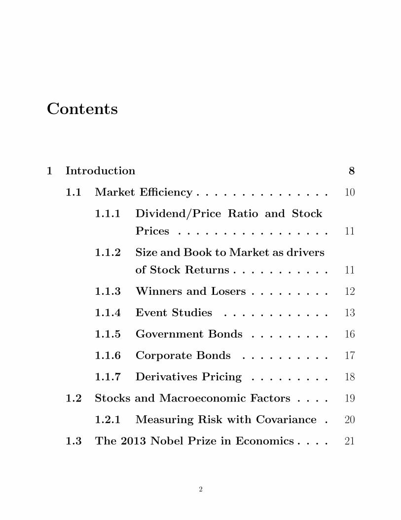
Contents
1 Introduction 8
1.1 Market Efficiency . . . . . . . . . . . . . . . 10
1.1.1 Dividend/Price Ratio and Stock
Prices . . . . . . . . . . . . . . . . . 11
1.1.2 Size and Book to Market as drivers
of Stock Returns . . . . . . . . . . . 11
1.1.3 Winners and Losers . . . . . . . . . 12
1.1.4 Event Studies . . . . . . . . . . . . 13
1.1.5 Government Bonds . . . . . . . . . 16
1.1.6 Corporate Bonds . . . . . . . . . . 17
1.1.7 Derivatives Pricing . . . . . . . . . 18
1.2 Stocks and Macroeconomic Factors . . . . 19
1.2.1 Measuring Risk with Covariance . 20
1.3 The 2013 Nobel Prize in Economics . . . . 21
2
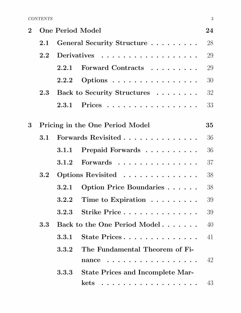
CONTENTS 3
2 One Period Model 24
2.1 General Security Structure . . . . . . . . . 28
2.2 Derivatives . . . . . . . . . . . . . . . . . . 29
2.2.1 Forward Contracts . . . . . . . . . 29
2.2.2 Options . . . . . . . . . . . . . . . . 30
2.3 Back to Security Structures . . . . . . . . 32
2.3.1 Prices . . . . . . . . . . . . . . . . . 33
3 Pricing in the One Period Model 35
3.1 Forwards Revisited . . . . . . . . . . . . . . 36
3.1.1 Prepaid Forwards . . . . . . . . . . 36
3.1.2 Forwards . . . . . . . . . . . . . . . 37
3.2 Options Revisited . . . . . . . . . . . . . . 38
3.2.1 Option Price Boundaries . . . . . . 38
3.2.2 Time to Expiration . . . . . . . . . 39
3.2.3 Strike Price . . . . . . . . . . . . . . 39
3.3 Back to the One Period Model . . . . . . . 40
3.3.1 State Prices . . . . . . . . . . . . . . 41
3.3.2 The Fundamental Theorem of Fi-
nance . . . . . . . . . . . . . . . . . 42
3.3.3 State Prices and Incomplete Mar-
kets . . . . . . . . . . . . . . . . . . 43
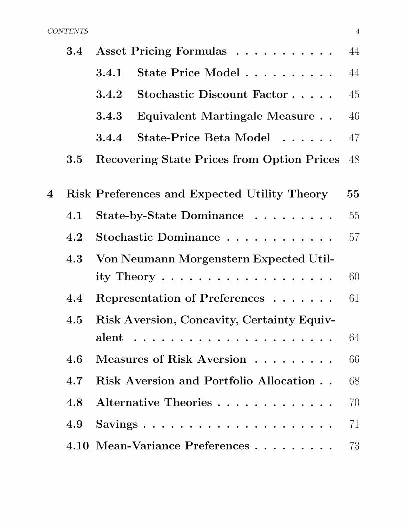
CONTENTS 4
3.4 Asset Pricing Formulas . . . . . . . . . . . 44
3.4.1 State Price Model . . . . . . . . . . 44
3.4.2 Stochastic Discount Factor . . . . . 45
3.4.3 Equivalent Martingale Measure . . 46
3.4.4 State-Price Beta Model . . . . . . 47
3.5 Recovering State Prices from Option Prices 48
4 Risk Preferences and Expected Utility Theory 55
4.1 State-by-State Dominance . . . . . . . . . 55
4.2 Stochastic Dominance . . . . . . . . . . . . 57
4.3 Von Neumann Morgenstern Expected Util-
ity Theory . . . . . . . . . . . . . . . . . . . 60
4.4 Representation of Preferences . . . . . . . 61
4.5 Risk Aversion, Concavity, Certainty Equiv-
alent . . . . . . . . . . . . . . . . . . . . . . 64
4.6 Measures of Risk Aversion . . . . . . . . . 66
4.7 Risk Aversion and Portfolio Allocation . . 68
4.8 Alternative Theories . . . . . . . . . . . . . 70
4.9 Savings . . . . . . . . . . . . . . . . . . . . . 71
4.10 Mean-Variance Preferences . . . . . . . . . 73

CONTENTS 5
5 General Equilibrium, Efficiency and the
Equity Premium Puzzle 77
5.1 Pareto Efficiency . . . . . . . . . . . . . . . 79
5.2 The Sharpe Ratio, Bonds and the Equity
Premium Puzzle . . . . . . . . . . . . . . . 81
5.3 Adding Expected Utility . . . . . . . . . . 83
5.4 The Equity Premium Puzzle . . . . . . . . 84
5.5 Empirical Estimation: Generalized Method
of Moments . . . . . . . . . . . . . . . . . . 85
6 Mean-Variance Analysis and CAPM 87
6.1 The Traditional Derivation of CAPM . . . 88
6.1.1 Two Fund Separation . . . . . . . . 95
6.1.2 Equilibrium leads to CAPM . . . . 96
6.2 The Modern Approach . . . . . . . . . . . 98
6.2.1 Pricing and Expectation Kernel . 102
6.2.2 Beta Pricing . . . . . . . . . . . . . 105
6.3 Testing CAPM . . . . . . . . . . . . . . . . 106
6.4 Practical Issues . . . . . . . . . . . . . . . . 107
6.4.1 Estimating Means . . . . . . . . . . 107
6.4.2 Estimating Variances . . . . . . . . 107
CONTENTS 6
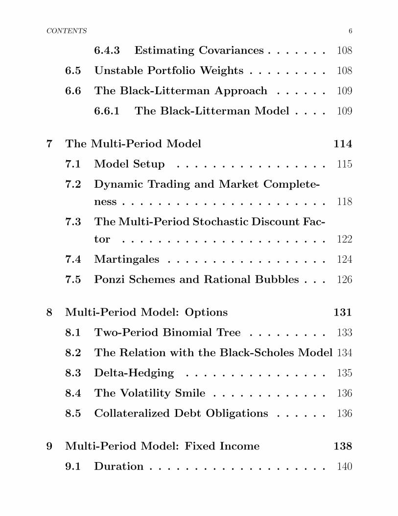
6.4.3 Estimating Covariances . . . . . . . 108
6.5 Unstable Portfolio Weights . . . . . . . . . 108
6.6 The Black-Litterman Approach . . . . . . 109
6.6.1 The Black-Litterman Model . . . . 109
7 The Multi-Period Model 114
7.1 Model Setup . . . . . . . . . . . . . . . . . 115
7.2 Dynamic Trading and Market Complete-
ness . . . . . . . . . . . . . . . . . . . . . . . 118
7.3 The Multi-Period Stochastic Discount Fac-
tor . . . . . . . . . . . . . . . . . . . . . . . 122
7.4 Martingales . . . . . . . . . . . . . . . . . . 124
7.5 Ponzi Schemes and Rational Bubbles . . . 126
8 Multi-Period Model: Options 131
8.1 Two-Period Binomial Tree . . . . . . . . . 133
8.2 The Relation with the Black-Scholes Model 134
8.3 Delta-Hedging . . . . . . . . . . . . . . . . 135
8.4 The Volatility Smile . . . . . . . . . . . . . 136
8.5 Collateralized Debt Obligations . . . . . . 136
9 Multi-Period Model: Fixed Income 138
9.1 Duration . . . . . . . . . . . . . . . . . . . . 140

CONTENTS 7
9.2 The Term Structure of Interest Rates . . 141
9.3 The Expectations Hypothesis . . . . . . . 141
9.4 Futures . . . . . . . . . . . . . . . . . . . . . 143
9.5 Swaps . . . . . . . . . . . . . . . . . . . . . . 145
10 The Multi-Period Equilibrium Model 149
10.1 Dynamic Hedging Demand INCOMPLETE 149
10.2 Intertemporal CAPM . . . . . . . . . . . . 150

Chapter 1
Introduction
Asset pricing is the study of the value of claims to uncertain future payments. Two components are
key to value an asset: the timing and the risk of its payments. While time effects are relatively
easy to explain, corrections for risk are much more important determinants of many assets’ values.
For example, over the last 50 years U.S. stocks have given a real return of about 9% on average.
Only about 1% of this can be attributed to interest rates; the remaining 8% is a premium earned
for holding risk.
This raises the question: what determines the price of financial claims? That is, why do prices move
over time, and why do different asset have different prices?1 There are several approaches that have
been used to answer these questions:
Statistical approaches look at statistical relationships between asset prices
“Weak” economic approaches look at some basic relations that must hold between asset prices,
such as the absence of risk-free profitable strategies2
Economic models derive prices from the fundamental characteristics of an economy3
Financial claims are promises of payments at various points in the future: for example, a stock is
a claim on future dividends; a bond is a claim over coupons and principal; an option is a claim
over the future value of another asset. More formally, suppose that we are at date t, then we can
we define payments xt+τ for τ ≥ 1 and expect the price of these payments to be something like
pt ≈ Et∑τ≥1
[xt+τ ], with some adjustment for time and risk. Another way to think about financial
claims is in terms of returns, defined as how much money we make if we hold an asset for a given
amount of time: Rt+1 = pt+1+xt+1
pt+1− 1. We call excess return the difference between the returns of
two assets i and j: Ret+1 = Ri,t+1 −Rj,t+1. We can interpret these three representations as follows:
1We will see that these questions refer to “time-series” and “cross-sectional” problems, respectively.2This concept is referred to as “no arbitrage”.3Such as preferences, technology, etc.
8

CHAPTER 1. INTRODUCTION 9
we can invest pt today and get xt+τ in the future, or invest 1 unit today and get Rt+1 in the
future, or yet invest 0 units today and get Ret+1 in the future. What are the properties of returns?
Can we predict when assets will have high or low returns? Can we predict which assets have higher
or lower returns? Historically, there have been two schools of thought on this subject:
The old view (1970s): Expected returns do not move much over time: stocks returns are
unpredictable because prices move with news about future cash-flows. The “classic” model for
asset pricing, called CAPM, works pretty well: returns with high covariance with the market
return have are higher on average as predicted by the mdoel. The beta parameter in the
CAPM model derives from the covariance between asset cash-flows and market cash-flows.
The modern view: Expected returns move a lot over time: stock returns are predictable.
Prices move with news about changes in the discount rate used by people to discount assets.
We can understand the cross-sectional relation between asset prices with multi-factor models:
characteristics other than the beta are associated with returns, and non-market betas matter
a lot. Finally, betas derive from the covariance between discount rates and market discount
rates.
Asset pricing theory can be used to describe both the way the world works and the way the world
should work. Once we observe the prices, we can use asset pricing theory to understand why prices
are what they are, and modify our theory if the predictions are not consistent with the observations;
or we can decide that the observed prices are wrong, or mispriced, and take advantage of the trade
opportunity. Much of asset pricing theory stems from one simple concept:
Price equals expected discounted payoff
The rest is elaboration, special cases and a few tricks. There are two approaches to this elaboration,
called absolute asset pricing and relative asset pricing . In absolute asset pricing we price
each asset by reference to its exposure to fundamental macroeconomic risk.4 This approach is
most popular in many academic settings in which we use asset pricing to give an explanation for
why prices are what they are in order to predict how prices might change if policy or economic
structure changed. In relative pricing we infer an asset’s value given the prices of some other asset.
Black-Scholes option pricing is the classic example of this approach.
The central and unfinished task of asset pricing theory is to understand and measure the sources of
aggregate risk that drive asset prices. Of course, this is also the central question of macroeconomics,
and in fact a lot of empirical work has documented stylized facts and links between macroeconomics
and finance. For example, expected returns vary across time and across assets in ways that are linked
to macroeconomic variables: we have learned that the risk premium on stocks5 is much larger than
4The classic examples of this approach are the Walrasian general equilibrium model discussed in Leon Walras’“Elements Of Pure Economics” (1877), and Gerard Debreu’s “Theory of Value” (1959).
5The difference between the stock return and the risk-free interest rate.

CHAPTER 1. INTRODUCTION 10
the interest rate, and varies a lot more than interest rates. This means that attempts to line up
investments with interest rates are vain, as much of the variation in cost of capital comes from
the varying risk premium. Similarly, we have learned that some measure of risk aversion must
be quite high, or people would all borrow like crazy to buy stocks. Moreover, while standard
macroeconomics theory predicts that agents do not care about business cycles,6 asset prices reveal
that they do: agents forgo substantial return premia to avoid assets whose value falls in recessions.
And yet theory still lags behind: we do not yet have a well-described model that fully explains these
correlations.
The rest of these notes is organized as follows. We start with frictionless markets and minimal
assumptions, adding more structure as the course progresses to obtain more and deeper implications.
In the second part of the course we will extend the discussion to multi-period settings, and finally
conclude by studying financial markets with frictions.
1.1 Market Efficiency
When is an asset fairly valued? We cannot answer this question without referring to a specific
model or assumption about the asset. Consider for instance the following assumption:
Prices incorporate and reflect all publicly available information
A direct consequence of this hypothesis is that stock returns should be unpredictable: for example,
when new information is released, stock prices should jump to the new fair level and then keep
trading around it. Are these features observed in reality? We will address this question with the
next subsections.
A related famous assumption is the Random Walk hypothesis, which states that stock market prices
evolve according to a random walk, and therefore cannot be predicted. This is compatible with the
Efficient Markets hypothesis outlined before, and it implies that stock price movements can only be
attributed to 1) news on future corporate cash flows, 2) changes in “risk premia” - the amount of
extra return that investors demand to hold risk (we will come back to this in the next lectures) or
3) shifts in behavioral bias.
Testing these hypotheses can be done in one of two main ways. One approach is to look at cross-
sectional data, that is, data collected at the same point in time, or regardless of differences in time.
Studies that use this approach look at whether some factors can explain the stock price changes,
potentially in contradiction to the efficient markets or random walk hypothesis. Another approach is
to look at time-series data, that is, data collected as a sequence of data points. Time-series studies
look into the existence of trends, seasonalities, or event-specific behaviors that would invalidate the
efficient markets or random walk hypothesis.
6Lucas (1987).
CHAPTER 1. INTRODUCTION 11
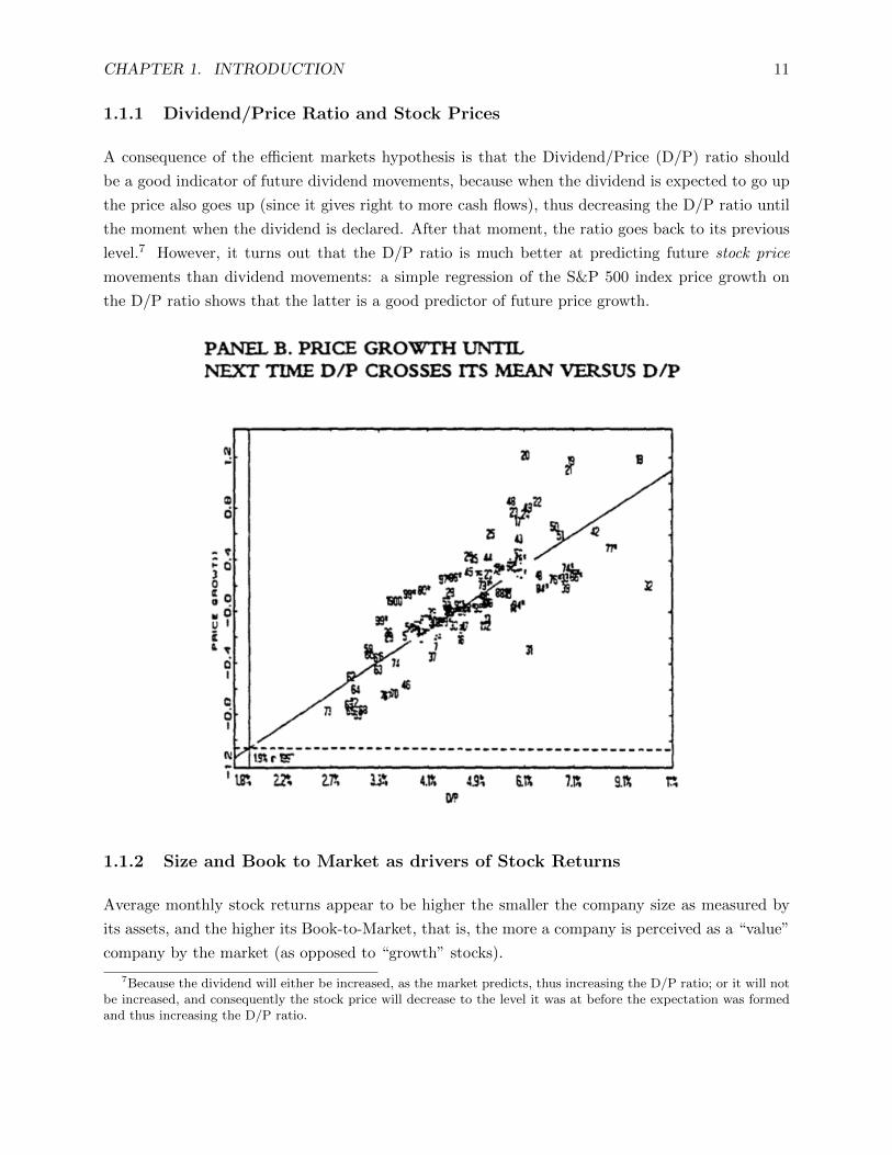
1.1.1 Dividend/Price Ratio and Stock Prices
A consequence of the efficient markets hypothesis is that the Dividend/Price (D/P) ratio should
be a good indicator of future dividend movements, because when the dividend is expected to go up
the price also goes up (since it gives right to more cash flows), thus decreasing the D/P ratio until
the moment when the dividend is declared. After that moment, the ratio goes back to its previous
level.7 However, it turns out that the D/P ratio is much better at predicting future stock price
movements than dividend movements: a simple regression of the S&P 500 index price growth on
the D/P ratio shows that the latter is a good predictor of future price growth.
1.1.2 Size and Book to Market as drivers of Stock Returns
Average monthly stock returns appear to be higher the smaller the company size as measured by
its assets, and the higher its Book-to-Market, that is, the more a company is perceived as a “value”
company by the market (as opposed to “growth” stocks).
7Because the dividend will either be increased, as the market predicts, thus increasing the D/P ratio; or it will notbe increased, and consequently the stock price will decrease to the level it was at before the expectation was formedand thus increasing the D/P ratio.

CHAPTER 1. INTRODUCTION 12
1.1.3 Winners and Losers
The average market-adjusted return for the strategy “buy and hold the n-th decile performing
stocks” shows a remarkable pattern: stocks that perform well over some time tend to underperform
in the following period (and vice versa), and this effect is stronger the better the past performance
(and vice versa). Over the medium-long term, mean-reversion appears to be a common feature in
stocks.8
8On the contrary, for shorter time-periods, momentum seems to drive prices more than mean-reversion.

CHAPTER 1. INTRODUCTION 13
1.1.4 Event Studies
What is the impact on daily stock returns of a company-specific event such as a merger, bankruptcy
or special dividend announcement? To find out, suppose we define as date t = 0 the date of the
anouncement of the financial event and calculate for each firm i the return Ri,t for t = −30, ..., 30.
Then we do the same for the market- or sector-reference group return, Rm,t to be used as comparison
and define abnormal returns as ARi,t = Ri,t − Rm,t. Finally, we consider the firms’ cumulative
average returns CAART =T∑
t=−30AARt, where AARt = 1
N
N∑i=1ARi,t: with no news at all, we expect
AARt to be close to zero. Below is a plot of the stylized possible reactions: an efficient reaction
is one in which the stock price maintains its new level after the event, an under-reaction is one in
which the stock price drifts up after the announcement, whereas in an over-reaction the stock price
drifts lower after the initial spike.

CHAPTER 1. INTRODUCTION 14
For instance, let us look at earning announcements. Ball and Brown (1968) show that there is not
only a pre-announcement drift, arguably due to insider information, but also a post-announcement
drift possibly due to the under- or over-reaction of the market to the earnings news released. This
constitutes a rejection of the Efficient Market Hypothesis even in its semi-strong form, which states
that stock prices reflect all publicly available information.
In a related paper, MacKinlay (1997) considers separately firms whose reported earnings were better,
equal or worse than expected earnings (as measured by the consensus estimate). Below is a plot of
their cumulative average abnormal returns: on average, over- and under-reactions are quite limited.
In a stock split, for each share held shareholders receive two shares. This usually signals that the
price has gone up far too much for small investors to be able to invest in the company, so firms

CHAPTER 1. INTRODUCTION 15
often decide to split the shares to make the investment more accessible to small investors. Normally
a stock split results in a price increase because many small investors can now buy the stock thus
driving the price up. Below is a plot of the cumulative average abnormal returns for the event of
the stock split: there are two possible explanations for this pattern. One is that inside information
is leaked prior to the announcement of the split. Another possibility however is that there is a
selection bias: only companies that perform well announce stock splits (those whose price increases
to a level unaccessible to small investors) and hence the pattern is due to selection bias.
Finally, below is a plot of cumulative average abnormal returns in the event of a take-over announce-
ment. Clearly, towards the announcement date there are signs of some leaked inside information,
and yet this is not completely factored in by the market since the price jumps on the announcement
date.

CHAPTER 1. INTRODUCTION 16
1.1.5 Government Bonds
The Expectation Hypothesis holds that that the long-term yield is determined by the market’s
expectation for the future short-term yield. According to EH, the term structure of interest rates
is fully determined by expectations about future short-term interest rates (and possibly maturity-
dependent risk premia). It can be stated in the following way:
Single-period holding returns on bonds of all maturities are equal in expectation
For example, holding a 5-year zero-coupon bond and selling it after 1 year gives you the same return
as holding a 1-year zero-coupon bond for 1 year. The one-year continuously compounded return on
a 1-year bond is:
r1,1 = Et[ln
1
Z(t, t+ 1)
]= ln
1
e−y(t,t+1)·1 = y(t, t+ 1)
While the one-year continuously compounded return on a m-year bond is:
r1,m = Et[lnZ(t+ 1, t+m)
Z(t, t+m)
]= Et
[lne−y(t+1,t+m)·(m−1)
e−y(t,t+m)·m
]= m·y(t, t+m)−(m−1)·Et [y(t+ 1, t+m)]
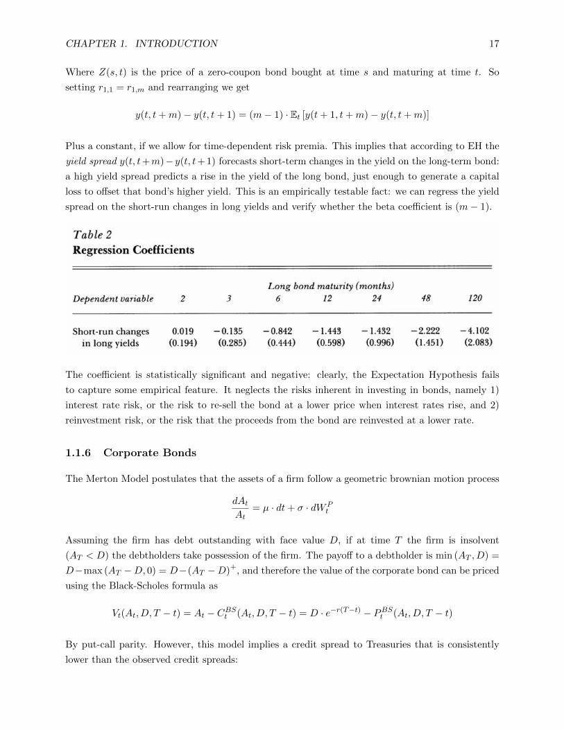
CHAPTER 1. INTRODUCTION 17
Where Z(s, t) is the price of a zero-coupon bond bought at time s and maturing at time t. So
setting r1,1 = r1,m and rearranging we get
y(t, t+m)− y(t, t+ 1) = (m− 1) · Et [y(t+ 1, t+m)− y(t, t+m)]
Plus a constant, if we allow for time-dependent risk premia. This implies that according to EH the
yield spread y(t, t+m)− y(t, t+ 1) forecasts short-term changes in the yield on the long-term bond:
a high yield spread predicts a rise in the yield of the long bond, just enough to generate a capital
loss to offset that bond’s higher yield. This is an empirically testable fact: we can regress the yield
spread on the short-run changes in long yields and verify whether the beta coefficient is (m− 1).
The coefficient is statistically significant and negative: clearly, the Expectation Hypothesis fails
to capture some empirical feature. It neglects the risks inherent in investing in bonds, namely 1)
interest rate risk, or the risk to re-sell the bond at a lower price when interest rates rise, and 2)
reinvestment risk, or the risk that the proceeds from the bond are reinvested at a lower rate.
1.1.6 Corporate Bonds
The Merton Model postulates that the assets of a firm follow a geometric brownian motion process
dAtAt
= µ · dt+ σ · dWPt
Assuming the firm has debt outstanding with face value D, if at time T the firm is insolvent
(AT < D) the debtholders take possession of the firm. The payoff to a debtholder is min (AT , D) =
D−max (AT −D, 0) = D−(AT −D)+, and therefore the value of the corporate bond can be priced
using the Black-Scholes formula as
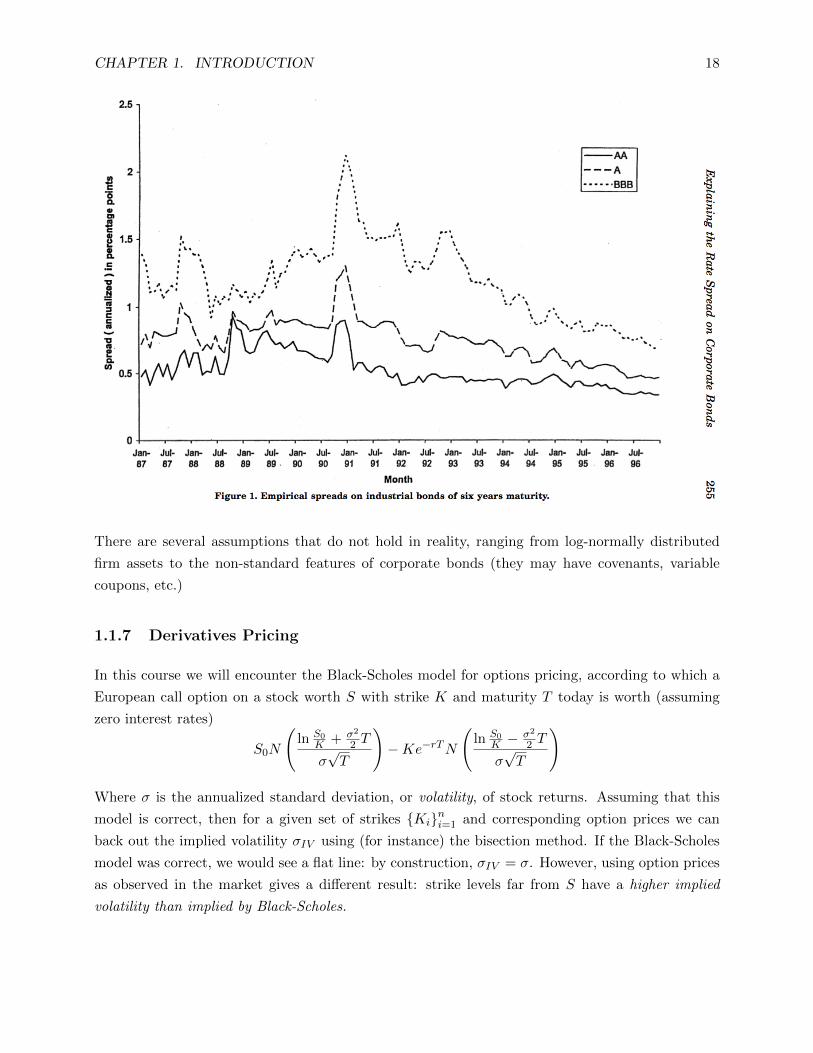
Vt(At, D, T − t) = At − CBSt (At, D, T − t) = D · e−r(T−t) − PBSt (At, D, T − t)
By put-call parity. However, this model implies a credit spread to Treasuries that is consistently
lower than the observed credit spreads:
CHAPTER 1. INTRODUCTION 18
There are several assumptions that do not hold in reality, ranging from log-normally distributed
firm assets to the non-standard features of corporate bonds (they may have covenants, variable
coupons, etc.)
1.1.7 Derivatives Pricing
In this course we will encounter the Black-Scholes model for options pricing, according to which a
European call option on a stock worth S with strike K and maturity T today is worth (assuming
zero interest rates)
S0N
(ln S0
K + σ2
2 T
σ√T
)−Ke−rTN
(ln S0
K −σ2
2 T
σ√T
)
Where σ is the annualized standard deviation, or volatility, of stock returns. Assuming that this
model is correct, then for a given set of strikes Kini=1 and corresponding option prices we can
back out the implied volatility σIV using (for instance) the bisection method. If the Black-Scholes
model was correct, we would see a flat line: by construction, σIV = σ. However, using option prices
as observed in the market gives a different result: strike levels far from S have a higher implied
volatility than implied by Black-Scholes.

CHAPTER 1. INTRODUCTION 19
Interestingly, this phenomenon became more evident after the 1987 Black Monday Crash. It has
been explained by the fact that rare events (crashes or rallies) occur more frequently in reality
than under the Black-Scholes model, hence the market incorporates that real feature of stocks by
“bidding the tails”.
We conclude this section with two empirical facts about stocks, macroeconomic factors, and how
risk measurements connect the two.
1.2 Stocks and Macroeconomic Factors
Let us begin by comparing the returns of a stock index and that of riskless bonds. The picture below
shows the return from investing $1 on January 1st 1972 in the S&P 500 index (red), a one-year
Treasury Bill (grey) and a 10-year Treasuty Note (brown). The return from the S&P 500 index has
been higher on average than both Treasury returns, yet much more volatile. The 1-year Treasury
Bill return is much lower and less volatile than the 10-year Treasury, a fact that is accounted for
by the relative size of their duration.

CHAPTER 1. INTRODUCTION 20
Similarly, looking at the yearly growth of the S&P 500 versus that of nominal GDP (which is mostly
comprised of consumption), we see that stocks are far more volatile than consumption.
1.2.1 Measuring Risk with Covariance
We will see that wisely managing a portfolio allows us to eliminate the stock-specific risk exposure.
What is left is the systemic risk, or market risk, which is captured by the covariance between the
stock and the market, and hence motivates us to use covariance as a risk measure for stocks. Below
is a plot of the covariance between some US large companies and the S&P 500.

CHAPTER 1. INTRODUCTION 21
1.3 The 2013 Nobel Prize in Economics
We conclude this chapter with an excerpt from the scientific background paper for the 2013 No-
bel Prize in Economics written by the Economic Sciences Prize Committee of the Royal Swedish
Academy of Sciences:
“While prices of financial assets often seem to reflect fundamental values, history provides striking
examples to the contrary, in events commonly labeled bubbles and crashes. Mispricing of assets
may contribute to financial crises and, as the recent recession illustrates, such crises can damage
the overall economy. Given the fundamental role of asset prices in many decisions, what can be
said about their determinants?
The 2013 Nobel prize was awarded empirical work aimed at understanding how asset prices are
determined. Eugene Fama, Lars Peter Hansen and Robert Shiller have developed methods toward
this end and used these methods in their applied work. Although we do not yet have complete and
generally accepted explanations for how financial markets function, the research of the Laureates has
greatly improved our understanding of asset prices and revealed a number of important empirical
regularities as well as plausible factors behind these regularities.
The question of whether asset prices are predictable is as central as it is old. If it is possible to
predict with a high degree of certainty that one asset will increase more in value than another
one, there is money to be made. More important, such a situation would reflect a rather basic
malfunctioning of the market mechanism. In practice, however, investments in assets involve risk,
and predictability becomes a statistical concept. A particular asset-trading strategy may give a high
return on average, but is it possible to infer excess returns from a limited set of historical data?

CHAPTER 1. INTRODUCTION 22
Furthermore, a high average return might come at the cost of high risk, so predictability need not
be a sign of market malfunction at all, but instead just a fair compensation for risk-taking. Hence,
studies of asset prices necessarily involve studying risk and its determinants.
Predictability can be approached in several ways. It may be investigated over different time hori-
zons; arguably, compensation for risk may play less of a role over a short horizon, and thus looking
at predictions days or weeks ahead simplifies the task. Another way to assess predictability is
to examine whether prices have incorporated all publicly available information. In particular, re-
searchers have studied instances when new information about assets becomes became known in the
marketplace, i.e., so-called event studies. If new information is made public but asset prices react
only slowly and sluggishly to the news, there is clearly predictability: even if the news itself was
impossible to predict, any subsequent movements would be. In a seminal event study from 1969,
and in many other studies, Fama and his colleagues studied short-term predictability from different
angles. They found that the amount of short-run predictability in stock markets is very limited.
This empirical result has had a profound impact on the academic literature as well as on market
practices.
If prices are next to impossible to predict in the short run, would they not be even harder to
predict over longer time horizons? Many believed so, but the empirical research would prove this
conjecture incorrect. Shiller’s 1981 paper on stock-price volatility and his later studies on longer-
term predictability provided the key insights: stock prices are excessively volatile in the short run,
and at a horizon of a few years the overall market is quite predictable. On average, the market
tends to move downward following periods when prices (normalized, say, by firm earnings) are high
and upward when prices are low.
In the longer run, compensation for risk should play a more important role for returns, and pre-
dictability might reflect attitudes toward risk and variation in market risk over time. Consequently,
interpretations of findings of predictability need to be based on theories of the relationship be-
tween risk and asset prices. Here, Hansen made fundamental contributions first by developing an
econometric method – the Generalized Method of Moments (GMM), presented in a paper in 1982
– designed to make it possible to deal with the particular features of asset-price data, and then
by applying it in a sequence of studies. His findings broadly supported Shiller’s preliminary con-
clusions: asset prices fluctuate too much to be reconciled with standard theory, as represented by
the so-called Consumption Capital Asset Pricing Model (CCAPM). This result has generated a
large wave of new theory in asset pricing. One strand extends the CCAPM in richer models that
maintain the rational-investor assumption. Another strand, commonly referred to as behavioral
finance – a new field inspired by Shiller’s early writings – puts behavioral biases, market frictions,
and mispricing at center stage.
A related issue is how to understand differences in returns across assets. Here, the classical Capital
Asset Pricing Model (CAPM) – for which the 1990 prize was given to William Sharpe – for a
long time provided a basic framework. It asserts that assets that correlate more strongly with

CHAPTER 1. INTRODUCTION 23
the market as a whole carry more risk and thus require a higher return in compensation. In a
large number of studies, researchers have attempted to test this proposition. Here, Fama provided
seminal methodological insights and carried out a number of tests. It has been found that an
extended model with three factors – adding a stock’s market value and its ratio of book value to
market value – greatly improves the explanatory power relative to the single-factor CAPM model.
Other factors have been found to play a role as well in explaining return differences across assets.
As in the case of studying the market as a whole, the cross-sectional literature has examined both
rational-investor–based theory extensions and behavioral ones to interpret the new findings.”
One last remark: Shiller and Fama’s works ultimately discuss the same findings, but interpreting
them differently. What Shiller calls irrational bubbles and behavioral biases Fama would call efficient
markets and varying risk premia is nothing but the empirical observation that the stochastic discount
factor varies a lot over time. Whether we label this as “irrational behavior” or “time-varying risk
premia” is an hypothesis that is very hard to test empirically.

Chapter 2
One Period Model
We begin our analysis of asset pricing by considering a simple setting in which there are two dates:
today (t = 0) and some future date (t = 1). We know everything about today’s state of the world
s = 0, but we don’t know which one of s = 1, ... , S states will materialize in the future.
Under this setup, we can represent a security j ∈ 1, ... , J as a vector
xj =
xj1...
xjS
and define a security structure by a matrix X:
X =
x11 x2
1 · · · xJ−11 xJ1
x12 x2
2 · · · xJ−12 xJ2
......
. . ....
...
x1S−1 x2
S−1 · · · xJ−1S−1 xJS−1
x1S x2
S · · · xJ−1S xJS
=[x1 x2 · · · xJ−1 xJ
]
An important example of a security structure is given by securities that are standard basis vectors,
which are called Arrow-Debreu securities. Consider for example S = 2 and e1 = (1, 0)′:
24

CHAPTER 2. ONE PERIOD MODEL 25
Note that if this is the only security available in the market, we can replicate any security in
the horizontal axis (e.g. the orange security above) by buying a quantity α ∈ R of e1, but we
cannot replicate any of the securities outside of the horizontal axis (e.g. the red security). When
the available securities are not enough to replicate all securities in RS we say that markets are
incomplete.
If we introduce another asset e2 = (0, 1)′, all securities in R2 become replicable. In this case, we say
that markets are complete. Note that adding another asset x3 ∈ R2 does not benefit us in any way,
as we were already able to span the whole set R2 with the previous two. The security structure
generated by e1 and e2 is
X =
(1 0
0 1
)
In general, given S possible states in t = 1 and J = S securities we call Arrow-Debreu security
structure the matrix
XAD =
1 0 · · · 0
0 1 · · · 0...
.... . .
...
0 0 · · · 1
Note that 1) all payoffs (securities) are linearly independent vectors in RS 2) markets are complete
by construction (since also J = S).
Consider now a general security structure in R2. Suppose there is only a riskless bond that pays 1
in each state of the world: b = (1, 1).

CHAPTER 2. ONE PERIOD MODEL 26
Under this security structure, all riskless securities on the 45 degree line are replicable (e.g. orange
security above) but none of the securities outside of it are replicable (e.g. 45 degree line). Adding a
risky security, say c = (2, 1)′, allows us to span the whole R2 set. For instance, suppose we wish to
replicate the security d = (1, 2)′. We can buy 3 securities b (in blue below) and sell short one unit
of security c (in orange), thus obtaining security d (in red):

CHAPTER 2. ONE PERIOD MODEL 27
Finally, notice that in the market structure considered here
X =[b c
]=
[1 2
1 1
]
b and c are linearly independent vectors in R2, and therefore the payoffs that can be obtained with
their linear combinations coincide with those that can be obtained with linear combinations of the
Arrow-Debreu securities e1 and e2 considered before: therefore, markets are complete.
Before going further, it is worthwile two three important remarks.
1) The state space itself is an important modeling choice. The relevance of this can hardly be over-
stated, because market completeness depends directly on how we specify the state space. Suppose
for example that the security structure looks like:
X =
1 0 9 4 2
2 1 5 2 2
3 1 8 4 9
4 2 1 2 2
4 2 1 2 2
Clearly markets are incomplete, but if the state s = 5 is a state of the world equivalent to s = 4
in all aspects with the only exception that “at noon my cat is on the third floor”, then state
s = 5 probably isn’t a relevant one and for modeling purposes should be disregarded. And after
eliminating state s = 5 markets are complete (in the relevant states s = 1, 2, 3, 4). Another example
where the state space choice is important is in derivatives pricing, where we assume that the state
space corresponds to the space of possible values of the underlying asset.
2) Although we said we would not deal with frictions until the third part of the course, market
incompleteness is a market friction: an incomplete market is equivalent to a market in which there
are infinite transaction costs to trade assets whose payoffs are inearly independent from the existing
assets, for which instead transaction costs are zero. From this point of view, we are dealing with a
very “black and white” setup: either we have no frictions at all (with market completeness) or an
extreme friction (with market incompleteness). Later in this course we will explore the “grey” area
in between.
Finally, trade limitations are another kind of market friction we will encounter in this part of the
course. Suppose there are only two states of the world and the security structure includes only a
riskless bond, which we can neitherbuy in large amounts nor short-sell (assume there is a law that
prohibits these practices):

CHAPTER 2. ONE PERIOD MODEL 28
Therefore, we can only achieve payoffs on the 45 degree line between the two yellow segments.
2.1 General Security Structure
We now have all the tools to formalize our analysis. We can define:
A Portfolio as a vector h ∈ RJ , whose entries represent a quantity for each asset in the
security structure.
The Portfolio Payoff is given byJ∑j=1
hjxj = Xh
The Asset Span is 〈X〉 =z ∈ RS : ∃h ∈ RJsuch that z = Xh
Note that it is always the case that 〈X〉 ⊆ RS , and we have market completeness if and only if
〈X〉 = RS , that is, if and only if rank(X) = S. In other words, market completeness refers to a
market structure in which there are at least S linearly independent assets. We say that security j
is redundant if there exists h ∈ RJ such that xj = Xh and hj = 0: when markets are complete and
J > S there are J − S redundant assets. When rank(X) < S markets are incomplete, and if there
are J < S linearly independent assets then S − J linearly independent assets are needed to achieve
market completeness.

CHAPTER 2. ONE PERIOD MODEL 29
2.2 Derivatives
While securities represent property rights (hence contracts), derivatives derive their value from an
underlying security. The most popular derivatives are Swaps, Futures and Options. A natural
question to ask is: since a derivative’s value is a function of the underlying security, are derivatives
always redundant assets? We will see that this is not the case in general, and the answer depends
on the fact that functional dependency does not imply linear dependency.
2.2.1 Forward Contracts
Forward contracts are binding agreements to buy or sell a given security at a specified price, quantity,
time and delivery logistics. Futures contracts are the same from a payoff point of view, but differ
from forwards because they are traded on exchanges that require collateral posting and hence are
more liquid.
The strike level is normally set so that the value of the contract at initiation is zero. Compared to
an outright long position in the underlying asset, it requires no cash outlay at initiation and gives
the same synthetic exposure to the underlying (that is, if the underlying ends up higher by 10 at
expiration, the forward will pay 10 as well). Assuming that a bond pays $1 at maturity, the relation
between a unit of the underlying and the corresponding forward contract is given by
Forward Contract V alue = V alue of Underlying − Strike×Bond

CHAPTER 2. ONE PERIOD MODEL 30
To see this, suppose the forward contract on a stock S is agreed at time 0 to buy an asset at a
future date T at a specified price K, so that the payoff is (ST −K). Now we ask: what is the fair
price of this contract today? If we can replicate this payoff with a combination of stocks and bonds
whose price is known today, we know that the price of the forward is going to be equal to the price
of that combination of stocks and bonds.
Suppose today we buy the stock at price S0, and sell K bonds maturing at T at a price of e−rT each.
What do we get at time T? The stock will be worth ST and each bond will be worth 1, so K bonds
will be worth K - since we sold them, we will have to pay K. In total, we have ST −K. Therefore we
replicated the payoff of the forward contract, and hence the price of the forward contract today will
be equal to the value of the portfolio of long 1 stock and short K bonds today, that is, S0−Ke−rT ,
that is, the value of the underlying asset minus the strike price times the bond price.
The forward contract can settle in one of two ways: 1) in cash, i.e. parties exchange the difference
between the underlying at maturity and the strike price in dollar value, which is less costtly and
more practical than 2) by physical delivery, i.e. parties exchange the underlying at the agreed
price. Credit risk can be an issue for over-the-counter forwards, for which credit checks and bank
letters of credit may be required other than collateral postings, while for exchange-based transaction
counterparty risk is reduced since the clearing house guarantees the transactions.
2.2.2 Options
A call option is a contract that gives the right (not the obligation) to buy an asset at a specified
price on a future date. From the point of view of the buyer, it preserves the upside potential from
owning an asset without the downside risk. The seller has an obligation to sell if the buyer chooses
to buy. The strike price is the price at which the parties agree to exchange the underlying. When
the buyer chooses to buy the asset, we say he exercises the option. The expiration date is the date
by which the buyer has to decide whether to exercise his right. Classified by exercise style, there
are three main classes of options: 1) European options can only be exercised at expiration date 2)
American options can be exercised anytime between inception and expiry and 3) Bermudan options
can be exercised during some specified dates before or on expiration date.
For European options, because the buyer only exercises when the spot price at maturity is higher
than the strike price (otherwise he would rationally buy the security in the market for less). There-
fore the payoff at expiration is given by
max S −K, 0 ≡ (S −K)+
and the profit is given by the payoff minus the future value of the option price, called option
premium.
Example: suppose you buy a 1-year call option on the S&P 500, currently trading at 1680, with
strike price 1700 and premium 197.34 dollars. Assuming a 5% one-year risk-free rate, if the index
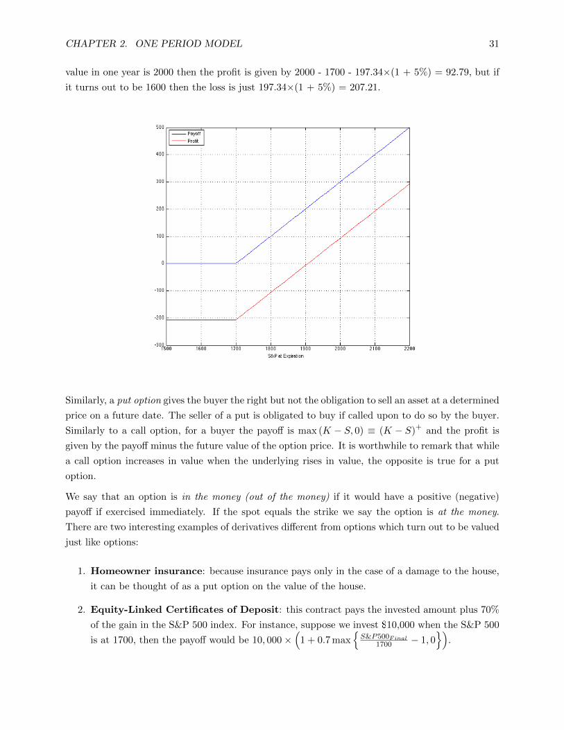
CHAPTER 2. ONE PERIOD MODEL 31
value in one year is 2000 then the profit is given by 2000 - 1700 - 197.34×(1 + 5%) = 92.79, but if
it turns out to be 1600 then the loss is just 197.34×(1 + 5%) = 207.21.
Similarly, a put option gives the buyer the right but not the obligation to sell an asset at a determined
price on a future date. The seller of a put is obligated to buy if called upon to do so by the buyer.
Similarly to a call option, for a buyer the payoff is max (K − S, 0) ≡ (K − S)+ and the profit is
given by the payoff minus the future value of the option price. It is worthwhile to remark that while
a call option increases in value when the underlying rises in value, the opposite is true for a put
option.
We say that an option is in the money (out of the money) if it would have a positive (negative)
payoff if exercised immediately. If the spot equals the strike we say the option is at the money.
There are two interesting examples of derivatives different from options which turn out to be valued
just like options:
1. Homeowner insurance: because insurance pays only in the case of a damage to the house,
it can be thought of as a put option on the value of the house.
2. Equity-Linked Certificates of Deposit: this contract pays the invested amount plus 70%
of the gain in the S&P 500 index. For instance, suppose we invest $10,000 when the S&P 500
is at 1700, then the payoff would be 10, 000×(
1 + 0.7 maxS&P500Final
1700 − 1, 0)
.
CHAPTER 2. ONE PERIOD MODEL 32
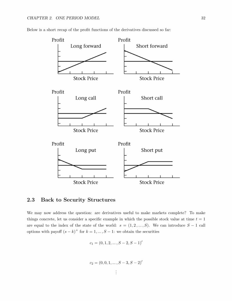
Below is a short recap of the profit functions of the derivatives discussed so far:
2.3 Back to Security Structures
We may now address the question: are derivatives useful to make markets complete? To make
things concrete, let us consider a specific example in which the possible stock value at time t = 1
are equal to the index of the state of the world: s = (1, 2 , ... , S). We can introduce S − 1 call
options with payoff (s− k)+ for k = 1, ... , S − 1: we obtain the securities
c1 = (0, 1, 2, ... , S − 2, S − 1)′
c2 = (0, 0, 1, ... , S − 3, S − 2)′
...

CHAPTER 2. ONE PERIOD MODEL 33
cS−1 = (0, 0, 0, ... , 0, 1)′
Which together with the stock give rise to the security structure
X =
1 0 · · · 0
2 1 · · · 0...
.... . .
...
S S − 1 · · · 1
This is an upper triangular S × S matrix whose determinant is one (the product of the terms on
the diagonal). Therefore X is full rank and markets are complete.
2.3.1 Prices
Let p ∈ RJ be the vector of prices for each asset. Then the cost of portfolio h is given by
p · h ≡J∑j=1
pjhj
and if pj 6= 0, the (gross) return vector for asset j is given by Rj = xj
pj.

CHAPTER 2. ONE PERIOD MODEL 34
Exercises
1) Using the Laplace expansion of the determinant of an S × S matrix, prove that
X =
1 0 · · · 0
2 1 · · · 0...
.... . .
...
S S − 1 · · · 1
Has determinant equal to 1.
2) Now repeat exercise 1 by adding to the security structure put options on the stock, following the
same steps as explained in the text (for call options). Are markets complete?
3) Suppose there exist only a risk-free asset x1 = (1, 1, . . . , 1)′ and a risky asset x2 6= x1 and S
states of the world. Let p1 and p2 be the prices of these two assets. A forward contract on the stock
is an agreement to pay an amount F at a future date t = T in exchange for the payment xjs when
the state s ∈ 1, 2, . . . , S realizes, with no cash flow exchange at time t = 0. Assuming arbitrage
opportunities are ruled out, find the fair value of F .
Chapter 3
Pricing in the One Period Model
Let us begin with some notation: for x, y ∈ Rn we write
y ≥ x if for each i = 1, ... , n yi ≥ xi
y > x if y ≥ x and y 6= x
y x if for each i = 1, ... , n yi > xi
y · x for the inner productn∑i=1xiyi
A fundamental concept in Asset Pricing is that of no arbitrage. In our setup it has three forms:
given any two portfolios h, k ∈ RJand a security structure X ∈ RS×J ,
1. Law of One Price: if Xh = Xk then p · h = p · k
2. No Strong Arbitrage: if Xh ≥ 0 then p · h ≥ 0
3. No Arbitrage: if Xh > 0 then p · h > 0
These definitions are related through the following lemmas:
Lemma 1: Law of One Price (LOOP) implies that every portfolio with zero payoff has
zero price.
Proof: grouping terms we can equivalently write X(h − k) = 0 ⇒ p · (h − k) = 0, and
therefore portfolio w ≡ h−k, which has zero payoff by construction, also has zero price.
Lemma 2: No Arbitrage (NA) implies No Strong Arbitrage (NSA).
Proof: trivial.
Lemma 3: NSA implies LOOP.
35

CHAPTER 3. PRICING IN THE ONE PERIOD MODEL 36
Proof: we prove the contrapositive “if LOOP does not hold, then NSA does not hold
either”. If the LOOP does not hold, then Xh = Xk and p ·h 6= p ·k. Assume p ·h < p ·k,
then we have X(h− k) = 0 ≥ 0 and p · (h− k) < 0, which is a violation of NSA for the
portfolio w ≡ h− k. Similarly, if p · h > p · k then X(k− h) = 0 ≥ 0 and p · (k− h) < 0,
again a violation of NSA for the portfolio q ≡ k − h.
3.1 Forwards Revisited
Consider the following payment and payoff timing combinations:
1. Outright purchase
2. Fully leveraged purchase: you borrow the money to execute the purchase
3. Prepaid forward: you pay today to receive shares in the future
4. Forward contract: you agree to a price now, which you pay when you receive the shares in
the future
3.1.1 Prepaid Forwards
Suppose we wish to price a prepaid forward for a stock with no dividends. Clearly the timing of
delivery is irrelevant, and the price of the prepaid forward F p0,T for a stock delivered at t = T is just
equal to the current stock price S0 at t = 0. This reasoning is called pricing by analogy.
Another way of getting to the same result is pricing by arbitrage. Suppose that at t = 0 we observe
that F p0,T > S0, then we could buy the stock today at S0, sell the forward at F p0 and pocket the
difference F p0,T −S0 > 0. In t = T our stock is worth ST , and we owe ST from the forward contract
we sold in t = 0: as a result, in t = T we receive 0. This would constitute an arbitrage. A similar
argument can be used for the case when F p0,T < S0. Therefore, absence of arbitrage requires that
F p0,T = S0.
When there are dividends the two pricing arguments do not hold any longer: the holder of the
stock, unlike that of the forward, will not receive dividends in the period [0, T ]. As a consequence,
it must be that F p0,T < S0 since F p0,T = S0 − PV (Dividend Payments in [0, T ]) . In particular:
With discrete dividends Dti for t1, ... , tn ∈ [0, T ] and assuming reinvestment at the risk-free
rate, we have F p0,T = S0 −n∑i=1PV0(Dti) = S0 −
n∑i=1Dtie
−rti
With continuous dividends with annualized dividend yield δ, we have F p0,T = S0e−δT
Note that this only applied to deterministic dividends: when dividends are stochastic the securities
structure turns from a matrix into a cube and we can no longer use our one period model.

CHAPTER 3. PRICING IN THE ONE PERIOD MODEL 37
3.1.2 Forwards
Obviously the forward price is just the future value of the prepaid forward:
With no dividends, F0,T = S0erT
With discrete dividends, F0,T = S0erT −
n∑i=1FVT (Dti) = S0e
rT −n∑i=1Dtie
r(T−ti)
With continuous dividends, F0,T = S0e(r−δ)T
Indexes are an example of assets with continuous dividends. We call forward premium the quantityF0,T
S0, which can be used to infer the current stock price from the forward price. The annualized
forward premium is π = 1T ln
F0,T
S0.
We can also use a no-arbitrage argument to price a forward: assuming continuous dividends with
rate δ, we can buy e−δT units of the stock worth S0 for total price of S0e−δT by borrowing the full
amount. At t = 0 there is no cash outlay; however, at t = T the portfolio is worth ST − S0e(r−δ)T .
Since the long forward payoff is ST −F0,T , this implies that to exclude arbitrage it must be the case
that F0,T = S0e(r−δ)T .
It follows that
Forward = Stock − Zero-Coupon Bond
An interesting application of this fact is the so-called cash and carry arbitrage: a market maker can
make a riskless profit by (for instance) selling short a forward contract and going long a synthetic
forward: the payoff from this strategy is F0,T − S0e(r−δ)T .
A natural question at this point is: is the forward price a market prediction of the future price?
The answer is no: the formula F0,T = S0e(r−δ)T shows clearly that the forward price provides no
more information than r, δ and S0.
CHAPTER 3. PRICING IN THE ONE PERIOD MODEL 38
3.2 Options Revisited
Consider two European options, one call and one put, with the same strike K and time to expiry
T . The put-call parity relation requires that
C(K,T )− P (K,T ) = PV0 (Forward Price− Strike) = e−rT (F0,T −K)
Note that if F0,T = K the long call short put portfolio above is equivalent to a synthetic forward,
and in fact will have zero price.1 With a dividend stream Dtini=1 we can rewrite the above relation
as
C(K,T )− P (K,T ) = S0 − PV0
(Dti
ni=1
)− e−rTK
While for an index (with continuous dividends) we have
C(K,T )− P (K,T ) = S0e−δT − e−rTK
3.2.1 Option Price Boundaries
Because an American option can be exercised at any time, while a European option can only be
exercised at maturity, it must be the case that
CA (K,T ) ≥ CE (K,T )
PA (K,T ) ≥ PE (K,T )
In general, the American call option price cannot exceed the stock price (otherwise you would never
buy the option but just buy the stock). Moreover, the European call option cannot be lower than
1) the price implied by put-call parity by setting to zero the put price, or 2) zero, whichever is
highest. That is,2
S0 > CA (K,T ) ≥ CE (K,T ) > e−rT (F0,T −K)+
Similarly, the American put option price cannot exceed the strike price (otherwise you would never
buy the option but just buy the bond). Moreover, the European put option cannot be lower than 1)
the price implied by put-call parity by setting to zero the call price, or 2) zero, whichever is highest.
That is,
K > PA (K,T ) ≥ PE (K,T ) > e−rT (K − F0,T )+
1An alternative definition of “At The Money” option is to say that an option is at the money when the forwardprice equals the strike price. Under this definition, a “long call short put” portfolio replicates a forward when the twooptions are at the money.
2Since maxe−rT (F0,T − S0) , 0
= e−rT (F0,T − S0)+ and CE (K,T ) > 0.
CHAPTER 3. PRICING IN THE ONE PERIOD MODEL 39
Rationally, we never exercise an American call option on a stock with no dividends: this is because3
CA (K,T ) ≥ CE (K,T ) = S0 −Ke−rT + PE(K,T ) =
= S0 −K +K(1− e−rT ) + PE(K,T )︸ ︷︷ ︸>0
> S0 −K
That is, for a holder of an American option it is always best to sell the option rather than exercise
it early. By LOOP, the price of an American call option on a stock with no dividends is the same
as that of an European option. Note that this is not true for a dividend-paying stock, as well as for
an American put on a non-dividend-paying stock.
3.2.2 Time to Expiration
An American option (both put and call) with more time to expiration is at least as valuable as
an American option with less time to expiration. This is because the longer option can easily be
converted into the shorter option by exercising it early. European call options on dividend-paying
stock and European puts may be less valuable than an otherwise identical option with less time to
expiration. A European call option on a non-dividend paying stock will be more valuable than an
otherwise identical option with less time to expiration.
3.2.3 Strike Price
Let K1 < K2, then we know that C(K1) ≥ C(K2) and P (K1) ≤ P (K2) (since their payoff is more
likely to be positive at t = T ). A less obvious fact is that C(K1) − C(K2) ≤ K2 − K1, because
the maximum payoff for a collar (long option with low strike, short option with high strike) with
strikes K1 < K2 is K2 −K1, and the price of the collar cannot exceed its maximum payoff. In the
same way, for put options we have P (K2)− P (K1) ≤ K2 −K1. Finally, the option price is convex
with respect to its strike: for K1 < K2 < K3,
C(K2)− C(K1)
K2 −K1≤ C(K3)− C(K2)
K3 −K2
Below is a brief recap of the put-call parity relations examined so far:
3Remember that with no dividends F0,T = S0erT .

CHAPTER 3. PRICING IN THE ONE PERIOD MODEL 40
To conclude, it is worthwile to note that many of these results on option price bounds can be
derived within our (very simple) two period model: they are incredibly robust. Once we adopt a
more specific settings (like the famous Black-Scholes model) we can use more sophisticated tools
such as needs dynamic replication, and the results become deeper but at the same time more hinging
on the specific model used.
3.3 Back to the One Period Model
So far we used prices of existing assets to directly derive the price (or price bounds) on other assets.
Now we will go along an indirect route: first we will derive the price of each individual state - called
state price - and then we will use this theoretical tool to derive the price of other assets.
For a given price vector p ∈ RJ and z ∈ 〈X〉 define the set v as
v(z) ≡ p · h : z = Xh
If LOOP holds then v is a linear functional, that is, a function mapping 〈X〉 onto R such that:
1. v is single-valued, because if Xh = z then by LOOP there exist only one p ∈ RJ such that
p · h = v, and therefore v is a singleton. This means that for any h ∈ RJ such that Xh ∈ 〈X〉we can write we can write v (Xh) = p · h.
2. v is linear on 〈X〉,4 since for any α, β ∈ R, z1 = Xh ∈ 〈X〉 and z2 = Xk ∈ 〈X〉 we have
αz1 + βz2 ∈ 〈X〉 and
αv(z1) + βv(z2) = αv(Xh) + βv(Xk) = αp · h+ βp · k = p · (αh+ βk) =
4That is, for all z1, z2 ∈ 〈X〉 and α, β ∈ R such that αz1 +βz2 ∈ 〈X〉 it holds that v(αz1 +βz2) = αv(z1) +βv(z2).

CHAPTER 3. PRICING IN THE ONE PERIOD MODEL 41
= v (X(αh+ βk)) = v (αXh+ βXk) = v (αz1 + βz2)
3. v(0) = 0, since Xh = 0 always has the solution h = 0 and because v is single-valued (by
LOOP) it must be that p · h = p · 0 = 0 is the only price of the payoff z = 0.
The converse is also true: if there exists a linear functional v defined in 〈X〉, then LOOP holds.
3.3.1 State Prices
Definition: a vector of state prices is a vector q ∈ RS such that p = X ′q.5
Definition: a linear functional V : RS → R is a valuation function if
1. V (z) = v(z) for every z ∈ 〈X〉
2. For every z /∈ 〈X〉, V (z) = q · z for q ∈ RS with qs = V (es): V extends v from 〈X〉 to RS .
Recall that es is the standard basis introduced in chapter 2: es ∈ RS is a vector with the sth
entry equal to 1 and all other entries equal to zero. The next proposition addresses the relationship
between v,V and q.
Proposition: if LOOP holds and q is a vector of state prices, then V (z) = q · z for
all z ∈ 〈X〉.
To see this we only need to show that also for z ∈ 〈X〉 we have V (z) = q · z (= v(z)). Suppose that
q is a vector of state prices and LOOP holds, then for z ∈ 〈X〉 we have
v (z) = p · h =
J∑j=1
pjhj =
J∑j=1
(xj · q
)hj =
J∑j=1
(S∑s=1
xjs · qs
)hj =
=
S∑s=1
J∑j=1
xjs · hj
qs =
S∑s=1
zsqs = q · z
Moreover the converse is also true, and therefore the valuation function V (z) = q · z is a linear
functional for all z ∈ RS if and only if q is a vector of state prices and LOOP holds.
Below is a graphical example of state prices. Given the securities structure (red arrows)
X =
(1 2
1 1
)5That is for j = 1, ... J we have pj = xj · q.
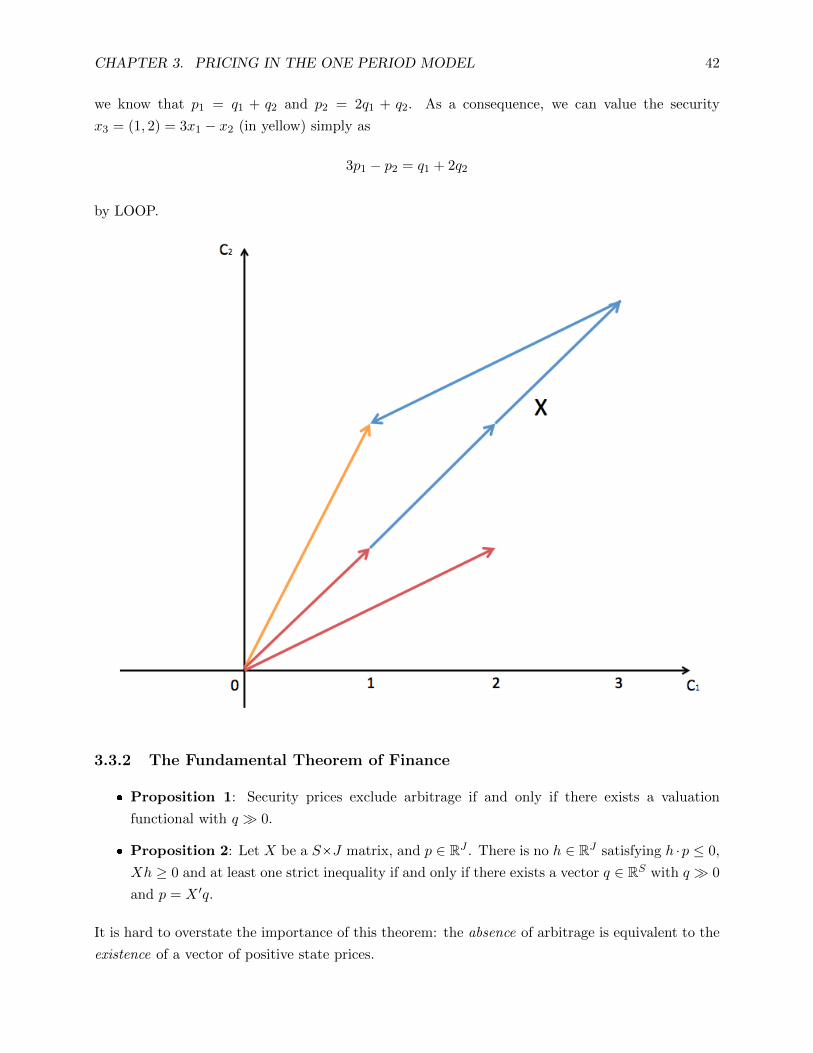
CHAPTER 3. PRICING IN THE ONE PERIOD MODEL 42
we know that p1 = q1 + q2 and p2 = 2q1 + q2. As a consequence, we can value the security
x3 = (1, 2) = 3x1 − x2 (in yellow) simply as
3p1 − p2 = q1 + 2q2
by LOOP.
3.3.2 The Fundamental Theorem of Finance
Proposition 1: Security prices exclude arbitrage if and only if there exists a valuation
functional with q 0.
Proposition 2: Let X be a SÖJ matrix, and p ∈ RJ . There is no h ∈ RJ satisfying h ·p ≤ 0,
Xh ≥ 0 and at least one strict inequality if and only if there exists a vector q ∈ RS with q 0
and p = X ′q.
It is hard to overstate the importance of this theorem: the absence of arbitrage is equivalent to the
existence of a vector of positive state prices.
CHAPTER 3. PRICING IN THE ONE PERIOD MODEL 43
3.3.3 State Prices and Incomplete Markets
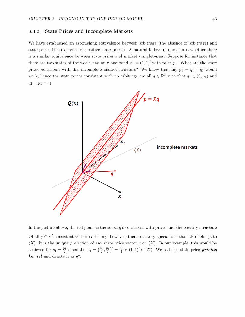
We have established an astonishing equivalence between arbitrage (the absence of arbitrage) and
state prices (the existence of positive state prices). A natural follow-up question is whether there
is a similar equivalence between state prices and market completeness. Suppose for instance that
there are two states of the world and only one bond x1 = (1, 1)′ with price p1. What are the state
prices consistent with this incomplete market structure? We know that any p1 = q1 + q2 would
work, hence the state prices consistent with no arbitrage are all q ∈ R2 such that q1 ∈ (0, p1) and
q2 = p1 − q1.
In the picture above, the red plane is the set of q’s consistent with prices and the security structure
Of all q ∈ R2 consistent with no arbitrage however, there is a very special one that also belongs to
〈X〉: it is the unique projection of any state price vector q on 〈X〉. In our example, this would be
achieved for q1 = p1
2 since then q =(p1
2 ,p1
2
)′= p1
2 × (1, 1)′ ∈ 〈X〉. We call this state price pricing
kernel and denote it as q∗.

CHAPTER 3. PRICING IN THE ONE PERIOD MODEL 44
Now we are ready to state the important relation between state prices and market completeness:
Proposition 3: Markets are complete and there is no arbitrage if and only if there exists a
unique valuation functional.
An intuitive proof of this proposition is the following: if markets are complete, then for a given
Xand p the system X ′q = p has a unique solution q ∈ RS+ (positivity follows from the assumption
of no arbitrage). If markets are not complete, then there exists a vector v ∈ RS such that v 6= 0
and Xv = 0. If there is no arbitrage, then there is a q 0 and some α ∈ R such that q + αv 0
and X(q + αv) = 0. Since this is also true for any fraction of α, it follows that there are infinitely
many state price vectors of the type q + αv.
3.4 Asset Pricing Formulas
We now present four asset pricing formulas. They are effectively equivalent, but each one can be
interpreted in a particular way and derived from the one period model.
3.4.1 State Price Model
This is just the pricing formula seen above: pj =S∑s=1
qsxjs

CHAPTER 3. PRICING IN THE ONE PERIOD MODEL 45
3.4.2 Stochastic Discount Factor
Analogously to the state price model, we can write pj =S∑s=1
πsqsπsxjs where π is the physical probability
distribution of states. Defining the random variable Stochastic Discount Factor as ms ≡ qsπs
, we get
pj =S∑s=1
πsmsxjs = E
[m · xj
].
Note that pj = E[m · xj
]= E
[xj]E [m] + Cov
[m,xj
], and since for a risk-free bond xbs = 1 for
alls, we have pb = E [m] = 1Rf
where Rf is the gross risk-free return. Therefore, for any asset j,
pj =E[xj]Rf
+ Cov[m,xj
]. Typically, Cov
[m,xj
]< 0.
Defining Rj ≡ xj
pj, we get E
[m ·Rj
]= 1. Since for a risk-free bond Rf = 1
E[m] , we can write
E[m ·
(Rj −Rf
)]= 0, or
E[m ·
(Rj −Rf
)]= E [m]
(E[Rj]−Rf
)+ Cov
(m,Rj
)= 0
That is,
E[Rj]−Rf = −
Cov(m,Rj
)E [m]
Which implies that the excess return for a generic asset j is determined solely by the covariance
with the stochastic discount factor. This also means that an investor is only compensated (with a
higher return) for holding systematic risk, not idiosyncratic risk.
Consider the stochastic discounf factor obtained from the pricing kernel m∗ ≡
q∗1π...q∗Sπ
. Note that m∗
is the projection of any stochastic discount factor m on 〈X〉, that is,
m∗ = proj (m| 〈X〉) ∈ 〈X〉
Which means that there exists a vector h∗ ∈ RJ such that m∗ = Xh∗. Therefore for any asset j we
can write
pj = E[m∗ · xj
]So for all assets we have
p = E[X ′m∗
]= E
[X ′Xh∗
]= E
[X ′X
]h∗
E [X ′X] is a second order moment: assuming it is invertible we can write
h∗ =(E[X ′X
])−1p

CHAPTER 3. PRICING IN THE ONE PERIOD MODEL 46
And therefore plugging this in m∗ = Xh∗ we obtain
m∗ = X(E[X ′X
])−1p
This is similar to the language of linear regressions. When we run a regression of p on
y = Xb+ ε
We find the linear combination of X that is “closest” to y by minimizing the varianc of the residual
ε. We do this by forcing the residual to be “orthogonal” to X, E [Xε] = 0. The projection of y
onto X is defined as the fitted value Xb = X (E [X ′X])−1 E [X ′y]. This idea is often illustrated by a
residual vector ε that is perpendicular to a plane defined by the variable X. Thus, when the inner
product is defined by a second moment, the operation “project y onto X” is a regression.
Finally, note that we can represent our previous discussion for state prices by shrinking the axes by
a factor√π:
3.4.3 Equivalent Martingale Measure
Starting again from pj =S∑s=1
qsxjs, for a riskless bond we have pb =
S∑s=1
qs = 11+rf
, where rf is
the risk-free net return. Thus we can write pj = 11+rf
S∑s=1
qsS∑s=1
qs
xjs = 11+rf
S∑s=1
πsxjs = 1
1+rfEQ [xj],
where πs ≡ qsS∑s=1
qs
.6 Compared to the stochastic discount factor approach, we simply used a different
6The Q notation comes from the literature about risk-neutral valuation.

CHAPTER 3. PRICING IN THE ONE PERIOD MODEL 47
probability measure to discount future states. We will see that the significance of this probability
measure is market-determined and its importance is paramount in options pricing theory.
3.4.4 State-Price Beta Model
Consider the stochastic discounf factor obtained from the pricing kernel m∗ ≡
q∗1π...q∗Sπ
, and define its
return as R∗ = m∗
pm∗≡ αm∗ for α > 0. Then we can write
E[Rj]−Rf = −
Cov(R∗, Rj
)E [R∗]
Defining βj ≡Cov(R∗,Rj)V ar(R∗) we can write for the asset j:
E[Rj]−Rf = −βj
V ar (R∗)
E [R∗]
While for security x∗
E [R∗]−Rf = −V ar (R∗)
E [R∗]
Therefore, for security j we have
E[Rj]−Rf = βj
(E [R∗]−Rf
)Which, if we assume a linear model for Rj and R∗ can be specified and tested empirically as
Rjk −Rf = βj
(R∗k −Rf
)+ εk
with Cov (R∗, ε) = E [ε] = 0.
In summary, the four equivalent pricing relations are:
1. State Price Model: pj =S∑s=1
qsxjs
2. Stochastic Discount Factor: pj = E[mxj
]3. Equivalent Martingale Measure: pj = 1
1+rfEQ [xj]
4. State-Price Beta Model: E[Rj]−Rf = βj
(E [R∗]−Rf
)As a last remark, note that whenever markets are incomplete, the multiplicity of state price vectors q
translates directly into the multiplicity of stochastic discount factors m and of equivalent martingale
measures π.

CHAPTER 3. PRICING IN THE ONE PERIOD MODEL 48
3.5 Recovering State Prices from Option Prices
Let’s assume for a moment that ST , the value of the asset at expiration, can take on a continuum
of values: at time t = T the stock price can have any value ST ∈ R+. In this section we will use the
law of one price to derive the price of an Arrow-Debreu security for a continuum of states, which is
a function q : R+ → R called state price density. In ths context, a state price density is the price of
an asset that pays one dollar in a particular state x ∈ R+ and zero in all others (here each value of
the price for the underlying asset at time t = T corresponds to a different state). Assuming further
that there exist call options offered in the market that cover a continuum of strike prices (one for
each possible outcome at expiration), the result of section 2.2.3 extends to this case: markets are
complete.
Fix a strike K > 0, and a (small) number ε > 0. Consider the following portfolio:
Buy x call options with strike K − ε
Sell 2x call options with strike K
Buy x call options with K + ε
State Payoff
ST ∈ [0,K − ε) 0
ST ∈ [K − ε,K) x (ST − (K − ε)) = x (ST −K) + xε
ST ∈ [K,K + ε) x (ST − (K − ε))− 2x (ST −K) = −x (ST −K) + xε
ST ∈ [K + ε,+∞) x (ST − (K − ε))− 2x (ST −K) + x (ST − (K + ε)) = 0
The payoff of this portfolio (symmetric butterfly) looks like the following:
This portfolio corresponds the payoff of an Arrow-Debreu security for state ST = K if two conditions
are satisfied:

CHAPTER 3. PRICING IN THE ONE PERIOD MODEL 49
1. The area under the payoff diagram (the sum of all possible payoffs) must be equal to one.
2. The option portfolio must yield a payoff of zero for all values of the underlying asset different
from K.
The area under the payoff diagram is equal to (xε)×(2ε)2 = xε2: to achieve (1), we set x = 1
ε2; to
achieve (2), we take the limit for ε→ 0. Now that we have replicated the payoff of an Arrow-Debreu
security, we can use the law of one price to determine the state prices: for a fixed ε > 0 the price
of the portfolio is
V (K, ε) =C (K + ε, T )− 2C (K,T ) + C (K − ε, T )
ε2
and therefore
q (K) = limε→0
V (K, ε) = limε→0
C (K + ε, T )− 2C (K,T ) + C (K − ε, T )
ε2=∂2C (K,T )
∂K2
We established an important fact: because q(K) > 0 if and only if ∂2C(K,T )∂K2 > 0, by the fundamental
theorem of finance there is no arbitrage if and only if for all K > 0 we have ∂2C(K,T )∂K2 > 0, that is,
if option prices are convex.
There is another important relationship related to state prices and ∂2C(K,T )∂K2 . We can write the
option price using the equivalent martingale measure representation as follows:
C (K,T ) = e−rTEQ [(ST −K)+]Taking the first derivative with respect to K we get
∂C (K,T )
∂K= −e−rTEQ [I ST −K ≥ 0] = −e−rTPQ ST ≥ K = −e−rT
(1− FQ
ST(K)
)Where FQ
STis the cumulative distribution function for the random variable ST under the equivalent
martingale measure Q.7 Differentiating again with respect to K we get
∂2C (K,T )
∂K2= e−rT fQST (K)
Together with our previous result,
∂2C (K,T )
∂K2= q(K) = e−rT fQST (K)
7We define I ST −K ≥ 0 as a function that is equal to one if ST − K ≥ 0 and zero otherwise. Note thatwe can take the partial derivative of C(K,T ) with respect to Ksince EQ [
(ST −K)+] =´R f
QST
(x) (x−K)+ dx =´∞KfQST
(x) (x−K) dx is smooth in K.

CHAPTER 3. PRICING IN THE ONE PERIOD MODEL 50
From the findamental theorem of finance, it follows that there exists a (positive) equivalent mar-
tingale measure density function fQST if and only if no arbitrage holds.
Note that this implies that we can evaluate any future payoff h(ST ) in 3 ways:
p = e−rTEQ [h (ST )] = e−rTˆRfQST (x)h (x) dx =
ˆR
∂2C (K,T )
∂K2(x)h (x) dx =
ˆRq(x)h (x) dx
Where the last term is the continuous-states equivalent of the formula p = Xq.
This means the following -apparently unrelated- conditions are equivalent:
Absence of arbitrage
Existence of a positive equivalent martingale measure density function
Convexity of options
Note that in the market we only directly observe the option prices for some discrete and finite set of
strikes: but if all the option prices C(K,T ) for the strikes K ∈ 0,∆, 2∆, . . . , N∆ are observable
(for N large and ∆ > 0 small enough) we can approximate ∂2C(K,T )∂K2 in the following way
∂2C (K,T )
∂K2≈ C (K + ∆, T )− 2C (K,T ) + C (K −∆, T )
∆2
and therefore we can also calculate the empirical market-implied probability distribution of ST ,
fQST , and the empirical state price density q.
Going back to our finite-state one-period model, if all the option prices C(s, T ) for the strikes
s ∈ 0, 1, 2, . . . , S are observable, we have
42C (s, T ) ≡ C (s+ 1, T )− 2C (s, T ) + C (s− 1, T ) = qs =πs
(1 + rf )
Appendix
The following is an alternative derivation from option prices of the state price density function. We
can construct the following portfolio: for some ε > 0 and δ > 0 and a fixed ST
Buy one call with strike ST − δ2 − ε
Sell one call with ST − δ2
Sell one call with ST + δ2

CHAPTER 3. PRICING IN THE ONE PERIOD MODEL 51
Buy one call with ST + δ2 + ε
If we buy 1ε units of this portfolio, when ST ∈
[ST − δ
2 , ST + δ2
]the total payoff is equal to 1. The
total value of this portfolio is
1
ε
[C
(K = ST −
δ
2− ε, T
)− C
(ST −
δ
2
)− C
(ST +
δ
2
)+ C
(ST +
δ
2+ ε
)]
Letting ε→ 0 this boils down to
−∂C(K = ST − δ
2 , T)
∂K+∂C(K = ST + δ
2 , T)
∂K
Finally, dividing by δ and letting δ → 0, we obtain the continuum-states version of a vector of state
prices, the state price density function ∂2C(K=ST ,T )∂K2 .
Suppose we want to evaluate a one-year “wedding cake option” of the type
Payoff =
$1, 000, 000 if ST ∈ [1700, 1750]
$0 otherwise
We now have the technology to price this. Its value will be equal to the integral of the state price
density over the interval [1700, 1750], that is, for T = 1,
ˆ 1750
1700
∂2C(K,T )
∂K2dK =
∂C (K = 1750, 1)
∂K− ∂C (K = 1700, 1)
∂K

CHAPTER 3. PRICING IN THE ONE PERIOD MODEL 52
Finally, note that this is equivalent to a portfolio comprising a long position in a binary 1700 call
and a short position in a 1750 binary call.

CHAPTER 3. PRICING IN THE ONE PERIOD MODEL 53
Exercises
1) Determine whether the following statements are true or false. Provide a proof or a counter-
example.
1. Law of one price and complete markets imply no strong arbitrage.
2. Law of one price and complete markets imply no arbitrage.
3. No strong arbitrage and complete markets imply no arbitrage.
2) Suppose there exist 3 states of the world s = 1, 2 and 2 assets x1, x2.
1. Suppose x1 = (2, 1, 0)′ and x2 = (0, 1, 0)′. Describe the asset span. Are markets complete?
2. Suppose p1 = 4 and p2 = 3. What type of no-arbitrage requirements does this market satisfy?
3. What are the restrictions on p1 and p2 such that this market satisfies LOOP, NSA and NA?
(Write each restriction separately)
4. Repeat 1), 2) and 3) for x1 = (1, 1, 0)′ and x2 = (0, 2, 0)′.
5. Repeat 1), 2) and 3) for x1 = (1, 1, 0)′, x2 = (0, 2, 0)′ and x3 = (0, 1, 1)′.
3) Suppose a stock index is currently trading at $300, the dividend yield on the index is 3% per
annum, and the risk-free interest rate is 8% per annum. What is the lower bound for the price of a
6-month European call option on the index when the strike price is $290?
Now assume a stock currently sells for $32. A 6-month call option with a strike of $30 has a
premium of $4.29, and a 6 month put with the same strike has a premium of $2.64. Assume a 4%
continuously compounded risk-free rate. What is the present value of dividends payable over the
next 6 months?
Finally, suppose a stock is priced at $23 per share. The interest rate is 7% per annum and the stock
pays no dividend. A three-month European call option with a strike price of $30 has a price of $0.3
What is the value of a European put with the same underlying asset, same strike price and same
time to expiration?
4) Suppose there are 3 call options traded on a stock with strike prices equal to 40, 50 and 60 and
with prices C(40) = 8, C(50) = 6 C(60) = 2.
1. Show that prices allow for arbitrage and provide an arbitrage portfolio with initial price equal
to zero. What kind of strategy is this?
2. Is it possible to exploit the arbitrage with a symmetric butterfly spread with zero initial price?

CHAPTER 3. PRICING IN THE ONE PERIOD MODEL 54
5) Suppose there exist 3 states of the world s = 1, 2, 3 and 2 assets x1 = (2, 1, 0)′ and x2 = (0, 1, 0)′.
1. Suppose p1 = 1 and p2 = 0.3. What state prices are consistent with these prices?
2. Solve for the unique pricing kernel q∗.
3. Use the pricing kernel to value a third asset x3 = (0, 1, 1)′. What other state prices (different
from q∗) are consistent with no arbitrage?
4. Now suppose p3 = 0.6. Solve for the state price vector. Does this market permit arbitrage?
5. Solve for the stochastic discount factor assuming the physical probability is such that π1 =
π2 = π3 = 13 .
6. Solve for the distribution under the equivalent martingale measure.
6) Suppose a stock index is currently trading at $25, and there are 5 possible states of the world in
t = T such that ST ∈ 15, 20, 25, 30, 35.
1. Given a zero risk-free interest rate, describe a valid equivalent martingale measure.
2. Under this measure, price call options at K = 15, 20, 25, 30, 35.
3. Use this information to recover state prices.
7) Suppose there are S possible states of the world in t = T and each has a (physical) probability
of occurrence ηs > 0 withS∑s=1
ηs = 1. Consider the vector µ ∈ RS with for s = 1, . . . , S µs = qsηs
,
where q is a state-price vector. Write E (y) =S∑s=1
ηsys for any y ∈ RS .
1. Consider an asset with payoff x = (x1, . . . , xS). Show that the price of this asset must be
E (z), where zs = µsxs. Interpret this result.
2. Let the rate of return for an asset with price p > 0 in state s be rs = xsp and let ws = rsµs.
Show that E (w) = 1. Is there some function of the excess return r− rf of the asset such that
E[f(r − rf )
]= 0?
8) Show in detail how to retrieve state prices using put options both in a continuous and discrete
states setup.
Chapter 4
Risk Preferences and Expected Utility
Theory
So far in this course we dealt with relative asset pricing: we derived asset prices through information
available on other, pre-existing assets. In this chapter we will study absolute asset pricing, a task
for which we have to specify the agents’ preferences towards risk. We will see that risk involves
knowledge of the probabilities of uncertain events, and agents’ attitude towards risk determines
how much they would be willing to pay for an asset - that is the core of absolute asset pricing.
A concept related to risk that we will not see in detail is that of uncertainty, which relates to the
agents’ preferences over events whose probability distribution is unknown.
It is important to stress that preferences over risk refer and are defined over “final payoff gambles”,
that is, after combining any random payoffs, such as the payoff of securities, investments, insurance,
and even non-random endowments.
We will start this chapter trying to answer the follwoing question: is there a criterion that allows
us to compare random payoffs?
4.1 State-by-State Dominance
A first attempt to answer this question is given by the principle of state-by-state dominance. Suppose
we have to choose one of the following three investments:
t = 0 t = 1
Initial CostProbabilities π1 = π2 = 1
2
s = 1 s = 2
Investment 1 -1000 1050 1200
Investment 2 -1000 500 1600
Investment 3 -1000 1050 1600
55

CHAPTER 4. RISK PREFERENCES AND EXPECTED UTILITY THEORY 56
It is hard to tell which one is better between investment 1 and 2: the two possible states they have
the same probability and in state 1 investment 1 pays more, while in state 2 investment 2 pays more.
However, investment 3 pays at least as much as investment 1 and 2 in any state of the world! Clearly
from this perspective investment 3 is more desirable, and we say that it state-by-state dominates
investments 1 and 2.
Definition (State-by-State Dominance): given two random variables X and Y
defined over the state space (Ω,F , P ), we say that Y state-by-state dominates X if
∀ω ∈ Ω X (ω) ≤ Y (ω).
We have already developed the notation needed to express state-by-state dominance: recall that for
x, y ∈ Rn we write
1. y ≥ x if for each i = 1, ... , n yi ≥ xi
2. y > x if y ≥ x and y 6= x
3. y x if for each i = 1, ... , n yi > xi
Assuming that x and y are scaled to have the same price, under any of the three conditions above
we would say that y state-by-state dominates x (you will notice that in the list above we see an
“increasing degree” of dominance).
A problem with state-by-state dominance is that it is an incomplete ranking: in fact, it is as
incomplete as RS . Another popular criterion which has been widely used is the mean-variance
dominance: assume that we like more expected return and less volatility. Consider the following
example:
t = 0 t = 1
Initial CostProbabilities π1 = π2 = 1
2
s = 1 s = 2 E [R] σ (R)
Investment 1 -1000 +5% +20% +12.5% 7.5%
Investment 2 -1000 -50% +60% +5% 55%
Investment 3 -1000 +5% +60% 32.5% 27.5%
Investment 1 has a higher expected return and lower volatility than investment 2. However, it is
not the case that investment 1 state-by-state dominates investment 2! Moreover, while investment
3 state-by-state dominates both investment 1 and 2, it only mean-variance dominates investment
2. Evidently, mean-variance dominance and state-by-state dominance are somehow unrelated or-
derings. However, while mean-variance dominance is an incomplete ranking, it does simplify the
problem of ranking investments to two dimensions only (it is as incomplete as R2). It looks like,

CHAPTER 4. RISK PREFERENCES AND EXPECTED UTILITY THEORY 57
potentially, a way of getting round the incompleteness problem is to find a criterion that amounts
to some number, for instance, in R, an ordered set. For example, suppose we rank investments
according to which Sharpe Ratio is highest:
Sharpe Ratio =E [R]− rf
σ (R)
In the example above, assuming rf = 3%, we get 1.27, 0.04 and 1.07 for investment 1, 2 and 3
respectively, and therefore we would select investment 1 (which, remember, we would eliminate
based on both state-by-state dominance and mean-variance dominance!)
Before going on, it is worthwile to remark that we can write the “payoff per state” representation
of random payoffs:
State s1 s2 s3 s4 s5
Probability π1 π2 π3 π4 π5
Payoff X 10 10 20 20 20
Payoff Y 10 20 20 20 30
in terms of “probability lotteries”:
Payoff 10 20 30
Probability X p10 = π1 + π2 p20 = π3 + π4 + π5 p30 = 0
Probability Y q10 = π1 p20 = π2 + π3 + π4 p30 = π5
This allows us to define preferences px py over probability distributions over states (rather than
on payoffs x y ∈ RS) and will turn out to be useful when thinking of final payoffs. Note that
we can always go from the“payoff per state” to the “probability lotteries” representation, but the
reverse is not true.
4.2 Stochastic Dominance
Another criterion to rank investment is the stochastic dominance. It is related to state-by-state
dominance, and is still an incomplete ordering of investments. Suppose there are two investment
opportunities 1 and 2:
Event e1 e2 e3
Payoff 10 100 2000
Probability 1 40% 60% 0%
Probability 2 40% 40% 20%

CHAPTER 4. RISK PREFERENCES AND EXPECTED UTILITY THEORY 58
In this case, every investment pays the same amount in each event, but the probabilities of the
events happening vary. To reconcile this with our previous “states of the world” discussion, it is
enough to note that the above example is such that investment 1 pays off 100 in the states s2 and s3
so that e2 = s2, s3, while investment 2 pays off 100 in state 2 and 2000 in state 3 (and obviously
e1 = s1).
Definition (First Order Stochastic Dominance): let FA and FB represent, re-
spectively, the cumulative distribution functions of two random variables (investments
payoff) defined in the interval [a, b]. We say that FA first-order stochastically dominates
(FSD) FB if ∀x ∈ [a, b] FA(x) ≤ FB(x).
Visually, FSD occurs whenever FA “stays below” FB for the whole domain. State-by-State Domi-
nance implies First Order Stochastic dominance.
Next, consider the following example:
Payoff 1 4 5 6 8 12
Probability 3 0% 25% 50% 0% 0% 25%
Probability 4 33% 0% 0% 33% 33% 0%
It is easy to verify that FSD does not hold for any investment. However, investment 3 is somewhat
special because its CDF stays below investment 4’s “most of the time”.
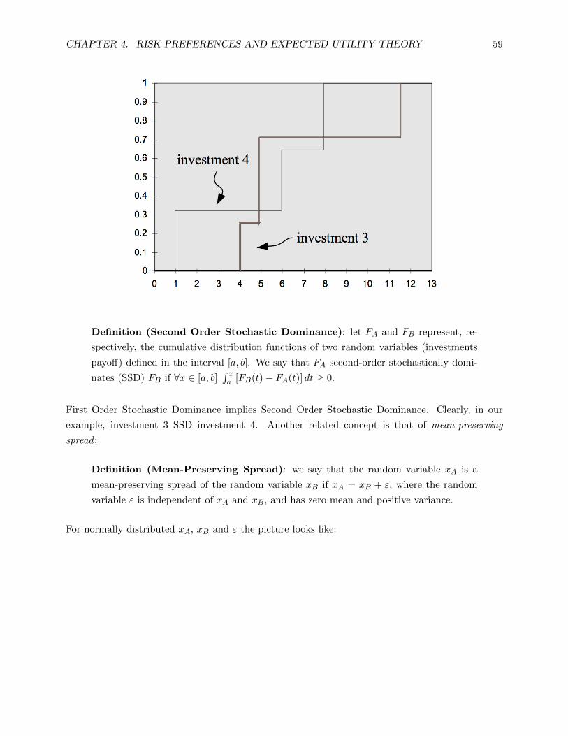
CHAPTER 4. RISK PREFERENCES AND EXPECTED UTILITY THEORY 59
Definition (Second Order Stochastic Dominance): let FA and FB represent, re-
spectively, the cumulative distribution functions of two random variables (investments
payoff) defined in the interval [a, b]. We say that FA second-order stochastically domi-
nates (SSD) FB if ∀x ∈ [a, b]´ xa [FB(t)− FA(t)] dt ≥ 0.
First Order Stochastic Dominance implies Second Order Stochastic Dominance. Clearly, in our
example, investment 3 SSD investment 4. Another related concept is that of mean-preserving
spread :
Definition (Mean-Preserving Spread): we say that the random variable xA is a
mean-preserving spread of the random variable xB if xA = xB + ε, where the random
variable ε is independent of xA and xB, and has zero mean and positive variance.
For normally distributed xA, xB and ε the picture looks like:

CHAPTER 4. RISK PREFERENCES AND EXPECTED UTILITY THEORY 60
The concept of mean preserving spread and that of second-order stochastic dominance are connected
by the following proposition:
Proposition: Let FA and FB be the CDFs of two random variables xA and xB defined
on the same space with identical means. Then FA SSD FB if and only if xA is a mean-
preserving spread of xB.
4.3 Von Neumann Morgenstern Expected Utility Theory
So far we mostly encountered criteria to rank uncertain payoffs which are incomplete, in the sense
that we can encounter two investments that we are unable to compare and decide which one is
better. We saw that this is linked to the fact that the criteria examined require to compare finite-
dimensional vectors (in the case of state-by-state dominance and mean-variance dominance) or
even functions, which can be considered as infinite-dimensional vectors (in the case of first and
second-order stochastic dominance). In this section we will elaborate another method which aims
at simplifying the problem by assigning to each investment a number u ∈ R, so that every two
investments are comparable. To do this by avoiding arbitrary choices of this function that maps
investments onto numbers, we will assume the existence of regular preferences over investments.
Let’s start with an example. Suppose you can enter the following bet: we flip a fair coin once. If
tails comes up, I’ll give you $1. If heads comes up, we’ll flip again, and if tails comes up I’ll pay
you $2, while if heads comes up we’ll flip again. Every time we flip again, the prize for a tails up
doubles. The question is: what is the fair price for this bet?
Since for the n-th flip the probability of a tails is(
12
)nand the payoff is 2n−1, and the number of

CHAPTER 4. RISK PREFERENCES AND EXPECTED UTILITY THEORY 61
flips ranges from 1 to infinity, it is straightforward to see that the expected payoff is
Expected Payoff =
∞∑n=1
(1
2
)n× 2n−1 =
∞∑n=1
1
2=∞
However this is the correct expected value, it does not make sense to pay all the money in the world
for this coin-flipping game (investment), since it pays you less that $64 in 99% of cases. Clearly this
criterion is inappropriate to value uncertain payoffs. This problem is was named the St. Petersburg
paradox and was first proposed by Daniel Bernoulli, who proposed the following solution: because
when you are rich an additional dollar is less valuable to you than when you are poor, we should
weight less the largest payoffs. He proposed to discount large payoffs using the natural logarithm:
introduce the parameter p for the denominator of the probability, in the previous example equal to
2. Then we can write:
Bernoulli V alue =
∞∑n=1
(1
p
)n× ln
(2n−1
)= ln 2
∞∑n=1
(n− 1)p−n =
1 = − ln 2∞∑n=1
(1− n)p−n = − ln 2∞∑n=1
d
dp
[p(1−n)
]= − ln 2
d
dp
[ ∞∑n=1
p(1−n)
]=
= − ln 2d
dp
[ ∞∑n=0
1
pn
]= − ln 2
d
dp
[1
1− p
]= ln 2
1
(1− p)2
Which for p = 2 is just ln 2. If the value is ln 2 and the function used to discount large payoffs is
the natural logarithm, we deduce that the price we are willing to pay for the coin-flipping game is
just x such that lnx = ln 2, that is, $2. Let’s dig deeper into this idea of specifying a function that
maps uncertain payoffs (investments) to a single number (utility).
4.4 Representation of Preferences
Suppose all we care about is consumption in each state. Then, the choice set would consist of vectors
in RS+1 where the first element represents consumption at t = 0, and all other elements represent
consumption in the possible S states at t = T . To reconcile this definition with our one-period
model, suppose an investor has an initial wealth W (constant across states and time) and is con-
sidering buying a security j with price pj and payoff xj . The vector(W − pj , (W − pj)× I + xj
)=
(c0, c1, ... cS)T ∈ RS+1 (where I is a S × 1 vector where each element is equal to one) would be the
corresponding consumption profile. Moreover, given two consumption profiles c, c′ ∈ RS+1, if an
investor chose c over c′ we say that that investor prefers c to c′ and write c c′.
Representation Theorem: Suppose the preference ordering is i) complete ii) tran-
sitive iii) continuous (and satisfies some further regularity conditions that we do not

CHAPTER 4. RISK PREFERENCES AND EXPECTED UTILITY THEORY 62
discuss here). Then the preference ordering can be represented by a utility function,
that is, c c′ if and only if there exists a utility function U such that U(c) > U(c′).
A related but different approach was developed by John Von Neumann and Oskar Morgenstern. In
this setup, we define the (finite) set of outcomes X (in the previous setup for instance, this was the
uncertain consumption profile at time t = T ) and we define a lottery as a probability measure over
X, that is a function p : X → [0, 1] such that 1) for x ∈ X p(x) ≥ 0 and 2)∑x∈X
p(x) = 1. The set
of all possible lotteries is
P ≡
p : X → [0, 1] |∀x ∈ X p(x) ≥ 0,
∑x∈X
p(x) = 1
Assume there exists a preference relation over P and consider the following three axioms:
Von Neumann - Morgenstern Axioms
1. (Regularity) Agents have complete and transitive preferences over P
2. (Independence) For any three lotteries p, q, r ∈ P and α ∈ (0, 1], p q ⇔ αp + (1 − α)r αq + (1− α)r
3. (Continuity) For any three lotteries p, q, r ∈ P such that p q r there exist α, β ∈ (0, 1)
such that αp+ (1− α)r q βp+ (1− β)r
Then the following theorem holds:
Theorem (Expected Utility Representation). If a preference relation over P satisfies
the Regularity, Independence and Continuity axioms, then there exists a function u :
X → R such that
p q ⇔∑x∈X
p(x)u(x) ≥∑x∈X
q(x)u(x)
That is, preferences over lotteries correspond to the expected utility of the lotteries. Below is a
graphical representation of an expected utility function over a lottery defined on a two-dimensional
state space:

CHAPTER 4. RISK PREFERENCES AND EXPECTED UTILITY THEORY 63
The 45° line represents the set of lotteries that pay off the same amount in both states. The
negatively sloped straight line is the set of lotteries in the (x1, x2) plane such that the expectation
of the lottery is equal to a value c > 0, that is, if π is the probability of the state 1 occurring,
c = πx1 + (1− π)x2, or x2 = π1−πx1 + c
1−π . The convex curve represents the indifference curve for
the agent: to give up a certain consumption amount in state 2, he is willing to take some amount
in state 1 to keep his utility level constant. The curve is the locus of lotteries in the (x1, x2) plane
such that k = πu (x1) + (1− π)u (x2), k ∈ R.
Going back to the axioms, consider the Independence axiom: it basically states that if we “dilute”
p and q with some third lottery r in the same way, but we prefer p to q, then our preference ranking
should not change. It can be visualized using trees:
However, this axiom rarely holds in experiments. For instance, suppose you are given the choice
between lottery p that pays $10 with probability 10% (and zero otherwise) and lottery q that pays
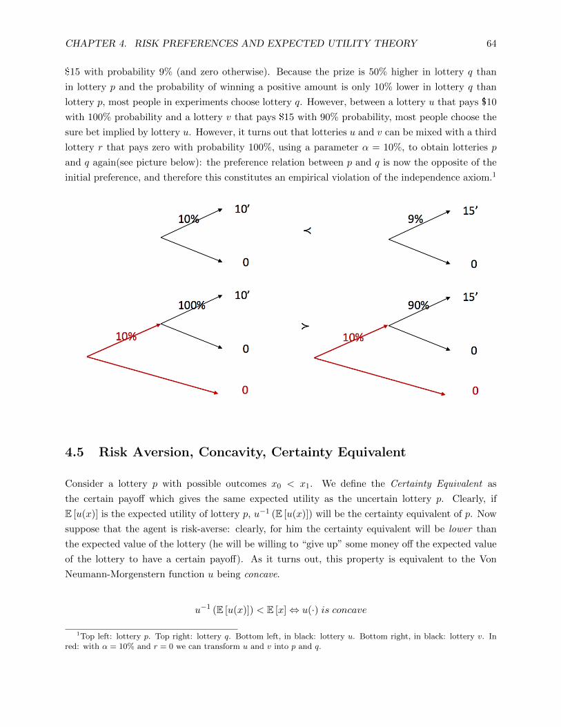
CHAPTER 4. RISK PREFERENCES AND EXPECTED UTILITY THEORY 64
$15 with probability 9% (and zero otherwise). Because the prize is 50% higher in lottery q than
in lottery p and the probability of winning a positive amount is only 10% lower in lottery q than
lottery p, most people in experiments choose lottery q. However, between a lottery u that pays $10
with 100% probability and a lottery v that pays $15 with 90% probability, most people choose the
sure bet implied by lottery u. However, it turns out that lotteries u and v can be mixed with a third
lottery r that pays zero with probability 100%, using a parameter α = 10%, to obtain lotteries p
and q again(see picture below): the preference relation between p and q is now the opposite of the
initial preference, and therefore this constitutes an empirical violation of the independence axiom.1
4.5 Risk Aversion, Concavity, Certainty Equivalent
Consider a lottery p with possible outcomes x0 < x1. We define the Certainty Equivalent as
the certain payoff which gives the same expected utility as the uncertain lottery p. Clearly, if
E [u(x)] is the expected utility of lottery p, u−1 (E [u(x)]) will be the certainty equivalent of p. Now
suppose that the agent is risk-averse: clearly, for him the certainty equivalent will be lower than
the expected value of the lottery (he will be willing to “give up” some money off the expected value
of the lottery to have a certain payoff). As it turns out, this property is equivalent to the Von
Neumann-Morgenstern function u being concave.
u−1 (E [u(x)]) < E [x]⇔ u(·) is concave
1Top left: lottery p. Top right: lottery q. Bottom left, in black: lottery u. Bottom right, in black: lottery v. Inred: with α = 10% and r = 0 we can transform u and v into p and q.

CHAPTER 4. RISK PREFERENCES AND EXPECTED UTILITY THEORY 65
And the difference E [x] − u−1 (E [u(x)]) is called Risk Premium. This fact derives directly from
Jensen’s Inequality:
Theorem (Jensen’s Inequality): Let g be concave over [a, b] and let x be a random
variable such that P [x ∈ [a, b]] = 1. If the expectations E [x] and E [g (x)] exist, then
E [g (x)] ≤ g (E [x]). Furthermore, if g(·) is concave then the inequality is strict.
The following theorems establish a relationship between First and Second Order Stochastic Domi-
nance and Expected Utility:
Theorem 1: Let FA and FB be two CDFs for the random payoffs x ∈ [a, b]. Then
FA FSD FB if and only if EA [U (x)] ≥ EB [U (x)] for all nondecreasing utility functions
U(·).
Theorem 2: Let FA and FB be two CDFs for the random payoffs x ∈ [a, b]. Then FA
SSD FB if and only if EA [U (x)] ≥ EB [U (x)] for all nondecreasing and concave utility
functions U(·).

CHAPTER 4. RISK PREFERENCES AND EXPECTED UTILITY THEORY 66
We conclude this subsetion with a parallel between (non-expected) utility representation and ex-
pected utility representation. In the former case, suppose U(c) = U (c0, c1, ... cS) represents a
complete, transitive and continuous preference ordering between consumption profiles. Then also
V (c) = f(U(c)), for f strictly increasing, represents the same preference ordering. In the latter case,
suppose that E [u(c)] represents a preference ordering satisfying the Von Neumann-Morgenstern ax-
ioms. Then for a, b ∈ R the affine function v(c) = a+ bu(c) represents the same preference ordering.
4.6 Measures of Risk Aversion
We define the following measures of risk aversion defined over the wealth Y of the agent:
1. Absolute Risk Aversion: RA(Y ) = −u′′(Y )u′(Y )
2. Relative Risk Aversion: RR(Y ) = −Y · u′′(Y )u′(Y ) = Y ·RA
3. Risk Tolerance: RT (Y ) = 1RA(Y )
There is an interesting link between expected utility and these measures of risk aversion: consider
the following lottery, where Y is the initial wealth of the agent:
What is the change in π needed for an agent to be indifferent when h rises? We can Taylor-expand
to the second degree the expected utility in a neighbourhood of Y to obtain:
π(Y, h) =1
2+
1
4hRA(Y ) + higher order terms
Similarly, consider the lottery

CHAPTER 4. RISK PREFERENCES AND EXPECTED UTILITY THEORY 67
Again, the change in π needed for an agent to be indifferent when h rises is obtained by Taylor-
expanding to the second degree the expected utility in a neighbourhood of Y to obtain:
π(Y, h) =1
2+
1
4θRR(Y ) + higher order terms
Similarly, suppose we add a small risk (lottery) x to the initial lottery w. Since E [u(w + x)] =
u(cCE
), we can use a second order Taylor expansion to show that
w − cCE ≈ RA(w)V ar(x)
2
Where w − cCE is the risk premium, and it is approximately linear in the variance of the additive
risk, with slope equal to half the coefficient of absolute risk aversion. Similarly, suppose we have
a multiplicative risk. Suppose that E [u(gw)] = u (kw), where g is a positive random variable with
unit mean and k is is the certainty equivalent growth rate. This time we get
1− k ≈ RR(w)V ar(g)
2
Therefore the coefficient of absolute risk aversion is relevant for additive risk, while the relative risk
aversion is relevant for multiplicative risk.
We will now introduce two specific functional forms for the Von Neumann-Morgenstern function U :
Constant Absolute Risk Aversion (CARA) utility function: U(x) = −e−ρY , for some ρ ∈ R+
Constant Relative Risk Aversion (CRRA) utility function: U(x) =
Y 1−γ
1−γ if γ 6= 1
lnY if γ = 1
For example, consider the CRRA utility and a lottery that adds $50,000 or $100,000 to the initial
wealth Y . The certainty equivalent is defined as the number CE ∈ R such that

CHAPTER 4. RISK PREFERENCES AND EXPECTED UTILITY THEORY 68
(Y + CE)1−γ
1− γ=
1
2× (Y + 50, 000)1−γ
1− γ+
1
2× (Y + 100, 000)1−γ
1− γ
For Y = 0 we get
γ = 0 CE = 75, 000 (risk neutrality)
γ = 1 CE = 70, 711
γ = 2 CE = 66, 246
γ = 5 CE = 58, 566
γ = 10 CE = 53, 991
γ = 20 CE = 51, 858
γ = 30 CE = 51, 209
While for Y = 100, 000 and γ = 5 the certainty equivalent is already 66,530 (close to γ = 2 for
Y = 0!)
4.7 Risk Aversion and Portfolio Allocation
Suppose that all assets are consumed in t = T , so that there are no savings in t = T . Moreover,
assume there is a riskless asset with net return rf and a risky asset with a random net return r.
We want to maximize the expected utility by choosing the risky asset allocation parameter a ∈ R:
maxa∈R
E[U(Y0
(1 + rf
)+ a
(r − rf
))]For some initial wealth Y0. The problem has first order conditions (FOC)
E[U ′(Y0
(1 + rf
)+ a
(r − rf
))(r − rf
)]= 0
We can characterize the solution to the problem with the following theorem:
Theorem: assume U ′ > 0, U ′′ < 0 and let a denote the solution to the problem above.
Then
a > 0⇔ E [r] > rf
a = 0⇔ E [r] = rf
a < 0⇔ E [r] < rf
Proof : define W (a) ≡ E[U(Y0
(1 + rf
)+ a
(r − rf
))], then the FOC can br written
as W ′(a) = 0. By risk aversion (that is, since U ′ > 0 and U ′′ < 0) we have W ′′(a) =
E[U ′′(Y0
(1 + rf
)+ a
(r − rf
)) (r − rf
)2]< 0, so W ′(a) is everywhere decreasing in a.

CHAPTER 4. RISK PREFERENCES AND EXPECTED UTILITY THEORY 69
This implies that a > 0 if and only if W ′(0) > 0, and since U ′ > 0 it follows that a > 0
if and only if E [r] > rf . The other assertions follow similarly.
How do measures of risk aversion depend on the initial wealth Y0? This is the subject of Arrow’s
theorem (1971):
Theorem 1: Let a = a (Y0) be the solution to the problem above. Then
∂RA∂Y0
< 0⇒ ∂a
∂Y0> 0
∂RA∂Y0
= 0⇒ ∂a
∂Y0= 0
∂RA∂Y0
> 0⇒ ∂a
∂Y0< 0
Theorem 2: If, for all wealth levels Y :
∂RR∂Y0
< 0⇒ da/a
dY/Y> 1
∂RR∂Y0
= 0⇒ da/a
dY/Y= 1
∂RR∂Y0
> 0⇒ da/a
dY/Y< 1
In the special case U(Y ) = lnY the FOC is
E[
r − rf
Y0 (1 + rf ) + a (r − rf )
]= 0
and assuming that r can take on two possible values r1and r2 with r1 < ff < r2, it is possible to
show thata
Y0=
(1 + rf
) (E [r]− rf
)(r2 − rf ) (rf − r1)
> 0
That is, a constant fraction of the initial wealth is invested in the risky asset. How does all this
generalize to the J assets case? The answer is provided by the following theorem:
Theorem (Cass and Stiglitz): Let the vectora1(Y0)
...
aJ(Y0)

CHAPTER 4. RISK PREFERENCES AND EXPECTED UTILITY THEORY 70
denote the amount optimally invested in the J risky assets if the initial wealth is Y0.
Then a1(Y0)
...
aJ(Y0)
=
a1
...
aJ
· f(Y0)
if and only if either i) U ′(Y0) = (θY0 + κ)∆ or ii) U ′(Y0) = ξe−vY0 .
In other words, it is sufficient to offer a mutual fund : the optimal proportion to invest in each asset
is given by the vector [a1, . . . , aJ ]T , and agents would then invest an amount depending on their
initial wealth level according to the function f (Y0).
To conclude this subsection, we generalize the class of utility functions by starting from the absolute
risk aversion (and then backing out the resulting utility function).
We call linear risk tolerance (or hyperbolic risk aversion) any utility function such that
RA = −u′′(c)
u′(c)=
1
A+B · c
Clearly, for B = 0 and A 6= 0 we have a CARA utility function. If B 6= 0 we obtain a generalized
power function
u(c) =1
B − 1(A+B · c)
B−1B
For which if B → 1 we obtain the log utility u(c) = ln (A+B · c), for B = −1 we obtain
the quadratic utility −12 (A− c)2, and for A = 0 we obtain the CRRA utility function u(c) =
1B−1 (B · c)
B−1B .
4.8 Alternative Theories
There are a number of theories alternative to Von Neumann-Morgenstern that have been proposed.
Savage’s expected utility theory (1954) combines the idea of utility function with subjective prob-
abilities, showing that under a set of axioms it is possible to derive subjective probabilities that
agents attach to events starting from their preferences over lotteries. This is considered an exten-
sion of the Von Neumann-Morgenstern paradigm, but like in vN-M it still suffers from the fact that
empirically its axioms are violated.
An interesting experiment that opened the door to ambiguity theory is Ellsberg’s paradox. Suppose
there are 10 balls in an urn and you have to make a choice between lottery 1 which pays you $100
if you pick a blue ball, and lottery 2 which pays you $100 if you pick a red ball, without knowing
how many balls are red or blue. Which one would you choose? Unlike preferences over risk, in this
case with uncertainty there are no probability distributions: it turns out that empirically people
are also uncertainty averse.

CHAPTER 4. RISK PREFERENCES AND EXPECTED UTILITY THEORY 71
Daniel Kahneman used insights from psychology to show that people first decide on a reference
point to compare outcomes with, and then consider lesser outcomes as losses and greater outcomes
as gains. In particular, he showed that empirically they are risk-averse in the gains domain, and
risk-loving in the loss space.
4.9 Savings
Within our one period model, consider an asset stucture composed of one risk-free asset with
constant gross return Rf . The agent has to make a decision on how much to consume in each
period t = 0 and t = T . If Rf increases, we will see two effects: one is the incentive to save more at
time t = 0, since by doing so we can now consume more in t = T -this is called substitution effect-
and the incentive to consume more (save less) at time t = 0, since the agent is effectively richer
when the gross riskless return increases -this is called income effect. In the log utility case, these
two effects cancel each other; in other cases (γ 6= 1) one effect can prevail over the other.
Suppose now there is a risk-free assets but the endowment in the future period is random. How does
the behavior of the agent change when we increase his exposure to risk? An old idea (going back
to J. M. Keynes) is that people save more when they face greater uncertainty. This phoenomenon
is called precautionary savings and it generally arises under two circumstances, one linked to the
shape of the utility function and one to the presence of borrowing constraints.
Let’s jump forward a little and suppose that in a multi-period setting agents maximize the expected
utility
E0
[ ∞∑t=0
βtu (ct)
]
subject to the intertemporal budget constraint
ct+1 = et+1 + (1 + r) (et − ct)
The standard Euler equation is
u′ (ct) = β (1 + r)Et[u′ (ct+1)
]And if u′′′ > 0, Jensen’s inequality implies
1
β (1 + r)=
Et [u′ (ct+1)]
u′ (ct)>u′ (Et [ct+1])
u′ (ct)
Which shows that the marginal rate of intertemporal substitution is higher in the presence of un-
certainty in ct+1. The difference between the two marginal rates, with and without uncertainty, is
attributed to precautionary savings. to see this, suppose the variance of et+1 increases (in a mean

CHAPTER 4. RISK PREFERENCES AND EXPECTED UTILITY THEORY 72
preserving fashion). Since numerator Et [u′ (ct+1)] is increasing in the variance of ct+1, in order for
the above equality to hold ct must decrease, that is, savings increase due to precautionary savings.
Suppose now there are no risk-free assets and one risky asset with random gross return R.
Theorem (Rothschild and Stiglitz): Let RA and RB be two return distributions
with identical means such that RB = RA + ε where ε is a white noise, and let sA and
sB be the savings out of Y0 corresponding to the return distributions of RAand RB
respectively. Then
If RR′ (Y ) ≤ 0 and RR (Y ) > 1, then sA < sB
If RR′ (Y ) > 0 and RR (Y ) ≤ 1, then sA > sB
Define Absolute Prudence as the quantity
PA(w) = −u′′′(w)
u′′(w)
and Relative Prudence as
PR(w) = −c · u′′′(w)
u′′(w)
Note that this depends directly on the curvature of u′ (u′′′ > 0 implies that u′ is convex) and does
not follow directly from risk aversion. It turns out that precautionary savings occur if P (w) > 0.
Moreover, we have the following result:
Theorem: Let RA and RB be two return distributions such that RA SSDRB, and let sA
and sB (respectively) be the savings out Y0. Then
sA ≥ sB ⇔ cP (c) ≤ 2
sA < sB ⇔ cP (c) > 2
Finally, agents might save precautionarily also because they are concerned that they will face
borrowing constraints in some state in the future: Bewley (1977) showed that with idiosyncratic
income shocks (borrowing constraints) negative mean asset holdings across individuals (mean[a]
below) result from simple individual optimization:

CHAPTER 4. RISK PREFERENCES AND EXPECTED UTILITY THEORY 73
4.10 Mean-Variance Preferences
A different approach is to specify the utility function over the mean-variance space of investment
returns. This is a much simpler approach than the Von Neumann-Morgenstern, so it is natural to
ask under which conditions the two approaches are equivalent. For instance, if all lotteries have
normally distributed prizes (not necessarily independent), because any linear combination of jointly
normal random variables is also jointly normal and therefore described by its first two moments,
expected utility can be expressed as a function of just mean and variance as well.
Another example in which mean variance and vN-M are equivalent is when agents have quadratic
utility:
u(y) = ay − by2
Then the expected utility is
E [u(y)] = aE [y]− bE[y2]
= aE [y]− bE [y]2 − bV ar (y)
Therefore, the expected utility is a function of the mean E [y] and variance V ar (y) only. This is also
true in another case: suppose all lotteries have normally distributed outcomes (thus the state space
now is infinite). Then, because any linear combination of normally distributed random variables
is also normal, the distribution of any lottery (or linear combination thereof) will be completely
described by its first two moments, mean and variance. Therefore also expected utility can be
expressed as a function of these two numbers only.

CHAPTER 4. RISK PREFERENCES AND EXPECTED UTILITY THEORY 74
Exercises
1) Using the definition in the chapter,
1. Show that state-by-state dominance implies first order stochastic dominance.
2. Provide a simple example of discrete, finite-state space random variables (that is, a table of
payoffs, states and probabilities) that can be ranked by first order stochastic dominance, but
not by state-by-state dominance.
2) Consider the random variables X ∼ N (0, 1) and Y ∼ N (1, 1).
1. Suppose Y = X + 1. What is the state-by-state ordering of X and Y (if any)? What is the
first-order stochastic dominance ordering of X and Y (if any)?
2. Suppose X and Y are independent random variables. What is the state-by-state ordering of
X and Y (if any)? What is the first-order stochastic dominance ordering of X and Y (if any)?
3. What conclusion can we draw about state-by-state and first order stochastic dominance in
relation to the probability distribution of the random variables?
3) Suppose an agent has an income of $10. He has the possibility to buy for $2 a lottery ticket
which pays the winner $19 (and zero otherwise). Suppose the agent has a von-Neumann Morgenstern
utility u (x) = ln (x) and believes that the probability of winning π is 13 .
1. Write the agent’s expected utility.
2. Should the agent buy the ticket?
3. Suppose the agent buys the ticket, but before a winner is selected he decides to sell it. What is
the minimum certain amount that the agent would accept in exchange for the lottery ticket?
4) To resolve the St.Petersburg Paradox, Bernoulli proposed to give less weight to large payouts in
the computation of the expected value of the game, to account for the fact that people value money
less and less the richer they become (though this certainly does not apply to MFins). This property
is shared by any increasing and concave function: can you guess why Bernoulli (a pretty smart guy)
proposed exactly u (x) = ln (x)? (Hint: consider the increase in utility u given by a small increase
in the payoff x)
5) Consider a general Von Neumann-Morgenstern utility function u(x) and a lottery which adds
an amount h to your personal wealth c in case of victory (which occurs with probability π) and
subtracts the same amount in case of loss:

CHAPTER 4. RISK PREFERENCES AND EXPECTED UTILITY THEORY 75
Show that the following relation holds:
π (c, h) =1
2+
1
4hRA (c) + o
(h2)
Similarly, consider a lottery which increases your personal wealth c by θ% in case of victory (which
occurs with probability π) and decreases your personal wealth by the same percentage amount in
case of loss:
Show that the following relation holds:
π (c, h) =1
2+
1
4θRR (c) + o
(θ2)
6) Consider adding a lottery x to lottery w. We know that teh certainty equivalent consumption is
defined by E [u(w + x)] = u(cCE
). Show that
w − cCE ≈ RA(w)V ar(x)
2
Similarly, for a positive random variable g with unit mean we have E [u(gw)] = u (kw), where k is
is the certainty equivalent growth rate. Show that
1− k ≈ RR(w)V ar(g)
2

CHAPTER 4. RISK PREFERENCES AND EXPECTED UTILITY THEORY 76
7) Suppose an agent is given the opportunity to enter, for free, a lottery that pays him $50,000
with probability 12 and $100,000 with probability 1
2 . Suppose the agent has CRRA utility
u (c) =c1−γ
1− γ
and γ = 7. Find the certainty equivalent of this lottery for the initial wealth Y equal to $0, $100,000
and $300,000. What happens to the certainty equivalent when the initial wealth increases? Interpret
this result.
8) Show that the solution to the portfolio optimization problem with one risky and one riskless
asset is such that agents invest a constant fraction of their wealth on the risky asset, and that this
results holds for any CRRA utility function and any distribution of the risky asset return r (please
refer to slide 51 in the slides set 4).
9) Show that the Ellsberg Paradox is a violation of the independence axiom (hint: build a compound
lottery).
10) Show that an agent with DARA preferences will choose to save precautionarily (hint: show
that the absolute prudence coefficient is positive).
11) Show that even if X and Y have positive skewness Z = X + Y can have negative skewness.
You can make any additional assumptions to prove your point. What does this fact depend on?
This shows that the negative skewness of the S&P 500 is consistent with single-name stocks having
positive skewness.

Chapter 5
General Equilibrium, Efficiency and
the Equity Premium Puzzle
In section 4.3 we introduced the representation of preferences over a consumption profile c =
(c0, c1, . . . , cS) ∈ RS+1+ . Suppose that, at birth, agent i is given an endowment e = (e0, e1, . . . , eS) ∈
RS+1+ and has a utility function U i : RS+1
+ → R. We say that U i is:
Quasiconcave, if the sets C = c : U(c) ≥ v are convex for each v ∈ R
Concave, if for any c, c′ ∈ RS+1 and α ∈ [0, 1] we have U i (αc+ (1− α)c′) ≥ αU i (c) + (1 −α)U i (c′)
Moreover, concavity implies quasiconcavity. If U i is also differentiable, a standard requirement is
that ∂U i
∂cs> 0 for each s = 0, 1, . . . S. We are now ready to formulate the portfolio consumption
problem:
maxc,h
U i (c0, c1, . . . cS)
Subject to the constratints
0 ≤ c0 ≤ e0 − p · h
0 ≤ cs ≤ es +J∑j=1
xjshj , s = 1, . . . , S
If we define cT ≡ (c1, . . . , cS) ∈ RS and eT ≡ (e1, . . . , eS) ∈ RS the latter constraint can be rewritten
more compactly as follows:
0 ≤ cT ≤ eT +Xh
The lagrangean for this problem is
L (c;λ, µ) = U i (c0, c1, . . . cS)− λ [c0 − e0 + p · h]− µ [cT − eT −Xh]
77

CHAPTER 5. GENERAL EQUILIBRIUM, EFFICIENCY AND THE EQUITY PREMIUM PUZZLE78
Note that X ′h = h′X and λ ∈ R, µ ∈ RS . Suppose c∗ solves the problem above, then there exist
λ ∈ R and µ ∈ RS such that:∂U i
∂c0(c∗) = λ (5.1)
∂U i
∂cs(c∗) = µs (5.2)
λp = µX (5.3)
The third FOC implies that
pj =S∑s=1
µsλxjs
Plugging in the first and second FOCs we have
pj =S∑s=1
∂U i/∂cs∂U i/∂c0
xjs
Assume that utility is time separable:
U i (c) = u (c0) + δu (cT )
And also that the utility over uncertain states u is a Von Neumann-Morgenstern utility:
U i (c) = u (c0) + δE [u (cT )]
Then we can rewrite our pricing relation as
pj =S∑s=1
πsδ∂ui/∂cs∂ui/∂c0
xjs
We can read our findings as follows:
δ ∂ui/∂cs
∂ui/∂c0is the stochastic discount factor ms
πsδ∂ui/∂cs∂ui/∂c0
= πsms is the state price qs
Thus, we are back to our equivalent asset pricing formulas
pj = xj · q = E[m · xj
]

CHAPTER 5. GENERAL EQUILIBRIUM, EFFICIENCY AND THE EQUITY PREMIUM PUZZLE79
Finally, note that the vector of marginal rates of substitutions ∂U i/∂cs∂U i/∂c0
is the state price vector (note
that this is positive by our assumption on U i).
5.1 Pareto Efficiency
Consider the set of allocations that yield agent i the same utility, S =c ∈ RS+1 : U i (c) = k
for
a given k ∈ R. This corresponds to a curve in the (c0, cs) space whose total differential is
∂U i (c)
∂c0dc0 +
∂U i (c)
∂csdcs = 0
called indifference curve of agent i. Equivalently,
∂U i/∂cs∂U i/∂c0
= −dc0
dcs≡MRSis,0
That is, the negative of the inverse of the slope dcsdc0
of the indifference curve is the marginal rate of
substitution MRSis,0 between consumption in state s = S and consumption in state s = 0 of agent
i. Moreover, we also know from the previous section that the marginal rate of substitution MRSs,0
equals the state price qs. We can represent this with an Edgeworth box : fix the consumption axes(cA0 , c
As
)for agent A with the origin in the lower left corner of the box, and draw a box that has
width equal to the sum of the endowments eA0 + eB0 in state 0 and height the sum of endowments
eAs + eBs in state s. We fix theconsumption axes(cB0 , c
Bs
)in the upper right corner of the box. The
endowments of the two agents corespond to a point e∗ = eA for the agent A axes, and e∗ = eB for
the agent B axes.

CHAPTER 5. GENERAL EQUILIBRIUM, EFFICIENCY AND THE EQUITY PREMIUM PUZZLE80
In the picture above, the indifference curves of agent A are in grey, while those of agent B are in
red. The dashed lines are the indifference curves that pass through the endowment eA (or eB if we
look at the agent B axes). The dash-dotted blue line represents the set of points in the Edgeworth
box for which MRSAs,0 = MRSBs,0, and is called contract curve. Allocations on this line are called
Pareto Optimal, that is, they are allocations with the property that there exists no other allocation
in the box such that at least one agent can be made better off without making someone else worse
off. It is important to remark that allocative efficiency (Pareto Efficiency) is not the same thing as
informational efficiency or fairness. The solid blue straight line has slope 1qs
and is the only straight
line passing from the endowment point for which MRSAs,0 = MRSBs,0 = qs. The point ce where
the straight blue line intersects the contract curve is called Competitive Equilibrium. The relation
between Pareto Optimality and Competitive Equilibrium is captured by the two Welfare Theorems:
1. First Welfare Theorem: If markets are complete, then the Competitive Equilibrium allo-
cation is Pareto Optimal.
2. Second Welfare Theorem: Any Pareto Efficient allocation can be decentralized as a Com-
petitive Equilibrium.
The First Welfare Theorem also implies that there exists a unique state price vector q and that for
any two agents i 6= j the vectors MRSi and MRSj (whose elements MRSis,0 for s = 1, . . . S) are

CHAPTER 5. GENERAL EQUILIBRIUM, EFFICIENCY AND THE EQUITY PREMIUM PUZZLE81
equal and coincide with q. However, in multi-period (or even multi-good) settings and markets are
incomplete, the equilibrium allocation is not Pareto Optimal.
We conclude the chapter with two interesting results about the aggregation of preferences:
Aggregation Theorem 1: Suppose markets are complete. Then asset prices in an
economy with K agents are identical to an economy with a single agent (social planner)
whose utility is
U(c) =
K∑k=1
αkuk(c)
Where αk is a weight given to agent k, uk is the utility of agent k and the single agent
consumes the aggregate endowment.
Aggregation Theorem 2: Suppose that i) a riskless annuity and the endowments
are tradable, ii) agents have common beliefs, iii) agents have a common rate of time
preference, iv) agents have Linear Risk Tolerance (LRT or Hyperbolic Risk Aversion)
preferences (see section 4.6) with
RkA(c) =1
Ak +Bc
Then asset prices in an economy with many agents are identical to a single agent economy
with LRT preferences such that
RA(c) =1
K∑k=1
Ak +Bc
5.2 The Sharpe Ratio, Bonds and the Equity Premium Puzzle
Consider a security with price pt at time t that pays off an amount xt+1 at time t + 1. Using the
SDF representation of the price we can write
pt = Et [mt+1xt+1] = Et [mt+1]Et [xt+1] + Covt [mt+1, xt+1]
Now, for a given (generic) mt+1 we write Rft = 1Et[mt+1] . If there exists a risk-free portfolio, Rft will
be unique and independent of the particular choice of mt+1. Therefore we have
pt =Et [xt+1]
Rft+ Covt [mt+1, xt+1]
Where the first term is the discounted expected payoff, and the second term is a risk adjustment.
Clearly, positive correlation of the payoff with the discount factor adds to the price (or, for a given

CHAPTER 5. GENERAL EQUILIBRIUM, EFFICIENCY AND THE EQUITY PREMIUM PUZZLE82
price, decreases the return on the asset). In returns we have
Et [mt+1Rt+1] = 1
And using Rft = 1Et[mt+1] we get
Et[mt+1
(Rt+1 −Rft
)]that is, the m-discounted expected return on any asset is equal to zero. This also implies
Covt
[mt+1, Rt+1 −Rft
]= −Et [mt+1]Et
[Rt+1 −Rft
]That is
Et[Rt+1 −Rft
]= −Covt [mt+1, Rt+1]
Et [mt+1]
so that we can see that the expected excess return, the risk premium, is determined by its covariance
with the stochastic discount factor. This also holds for a generic portfolio h ∈ RJ :
Et[(Rt+1 −Rft
)h]
= −Covt [mt+1, Rt+1h]
Et [mt+1]= −ρt (mt+1, Rt+1h)σt (mt+1)σt (Rt+1h)
Et [mt+1]
Note that all results hold also for the unconditional expectation E [·], so we can drop the expectation
subscript:
E[(Rt+1 −Rft
)h]
= −Cov [mt+1, Rt+1h]
E [mt+1]= −ρ (mt+1, Rt+1h)σ (mt+1)σ (Rt+1h)
E [mt+1]
Rearranging in terms of the portfolio Sharpe Ratio,
−σ (mt+1)
E [mt+1]ρ (mt+1, Rt+1h) =
E[(Rt+1 −Rft
)h]
σ (Rt+1h)
taking the absolute value of both sides,
σ (mt+1)
E [mt+1]|ρ (mt+1, Rt+1h)| =
∣∣∣∣∣∣E[(Rt+1 −Rft
)h]
σ (Rt+1h)
∣∣∣∣∣∣but since for any h ∈ RJ ρ (·) ∈ [−1, 1],
σ (mt+1)
E [mt+1]≥ sup
h∈RJ
∣∣∣∣∣∣E[(Rt+1 −Rft
)h]
σ (Rt+1h)
∣∣∣∣∣∣we just proved the following theorem:

CHAPTER 5. GENERAL EQUILIBRIUM, EFFICIENCY AND THE EQUITY PREMIUM PUZZLE83
Theorem (Hansen-Jagannathan Bound): The ratio of the standard deviation
of a stochastic discount factor to its mean exceeds the Sharpe Ratio attained by any
portfolio.
This theorem can be used to easily check the viability of a proposed stochastic discount factor. Or,
for a given stochastic discount factor, it establishes the maximum Sharpe Ratio any portfolio can
attain. Note that the theorem also holds for the expectation conditional at time t.
5.3 Adding Expected Utility
Now assume that agents maximize their expected utility. For c0 ∈ R and c1 ∈ RS ,
U (c0, c1) =S∑s=1
πsu (c0, c1,s)
so that
∂0u =
(∂u (c0, c1,1)
∂c0, . . . ,
∂u (c0, c1,S)
∂c0
)
∂1u =
(∂u (c0, c1,1)
∂c1, . . . ,
∂u (c0, c1,S)
∂cS
)and the stochastic discount factor can be shown to be m = MRS
π = ∂1uE[∂0u] ∈ RS . If the utility is also
time-separable, then u (c0, c1,s) = v (c0) + v (c1,s) and
∂0u =∂v (c0)
∂c0× (1, . . . , 1) = v′ (c0)× (1, . . . , 1)

CHAPTER 5. GENERAL EQUILIBRIUM, EFFICIENCY AND THE EQUITY PREMIUM PUZZLE84
∂1u =
(∂v (c1,1)
∂c1, . . . ,
∂v (c1,S)
∂cS
)=(v′ (c1,1) , . . . , v′ (c1,S)
)and therefore ms = 1
πs× πsv′(c1,s)
v′(c0) =v′(c1,s)v′(c0) . For example, suppose u (c0, c1,s) = ln c0 + ln c1,s. Then
m =
(c0
c1,1, . . . ,
c0
c1,S
)′
which shows that states where consumption is low are states in which m is high.
5.4 The Equity Premium Puzzle
Recall that for any asset j
E[Rj]−Rf = −Rf × Cov
[m,Rj
]Using the assumptions from the last section we can write
E[Rj]−Rf = −Rf ×
Cov[∂1u,R
j]
E [∂0u]
so the Hansen-Jagannathan bound can be rewritten as
σ (m) ≥ 1
Rf
∣∣∣∣∣E[Rj −Rf
]σ (Rj)
∣∣∣∣∣that is,
σ
(∂1u
E [∂0u]
)≥ 1
Rf
∣∣∣∣∣E[Rj −Rf
]σ (Rj)
∣∣∣∣∣However:
1. The right hand side of this inequality, the Sharpe Ratio of any asset, can be very high for
some portfolios.
2. Consumption volatility is generally low.
Together, to be consistent with the Hansen-Jagannathan bound these two facts imply that the
curvature of the utility function u must be very high. But curvature is synonimous for risk aversion,
and to justify the empirical data we should accept that agents have an unrealistically high level of
risk aversion. This inconsistency between theory and empirical facts is commonly referred to as the
Equity Premium Puzzle.

CHAPTER 5. GENERAL EQUILIBRIUM, EFFICIENCY AND THE EQUITY PREMIUM PUZZLE85
Even if we allowed for an unrealistically high level of risk aversion, more problems emerge: due to
the high degree of concavity of u there is also a low elasticity of intertemporal substitution (EIS)
which would drive agents to strongly smooth consumption over time. But in the context of a von-
Neumann Morgenstern utility function smoothing over time is equivalent to smoothing over states,
and in the example of a CRRA utility function, the EIS parameter is just 1γ . Finally, the puzzle
can be re-cast in terms of the risk-free interest rate, which the model predicts to be much higher
than in reality.
Solutions to the puzzles have been proposed, which essentially depart from the von-Neumann Mor-
genstern expected utility paradigm and allow for a utility representation that separates risk-aversion
from intertemporal elasticity of substitution.
5.5 Empirical Estimation: Generalized Method of Moments
Another great contribution by Lars Hansen (one of the 2013 Nobel Prize in Economics recipi-
ents) was the Generalized Method of Moments and its applications in the context of the canonical
consumption-based asset pricing model. We know that under CRRA utility we have
Et
[β
(Ct+1
Ct
)−γ (Rt+1 −Rft
)]= 0
That is, the expected discounted excess return should always be zero. How do we take this to data?
How do we find parameters beta and gamma that best fit the data? How do we check this over
many different times and returns, to see if those two parameters can actually explain empirical
facts? What do we do about that conditional expectation Et, conditional on information in people’s
heads? How do we bring in all the variables that seem to forecast returns over time (e.g. by the
dividend-price ratio) and across assets (value, size, etc.)? How do we handle the fact that return
variance changes over time, and consumption growth may be autocorrelated?

CHAPTER 5. GENERAL EQUILIBRIUM, EFFICIENCY AND THE EQUITY PREMIUM PUZZLE86
When Hansen wrote his paper, this was a big headache. He suggested to just multiply by any
variable z that we think forecasts returns or consumption, and take the unconditional average of
this conditional average: the model predicts that the unconditional average obeys
E
[β
(Ct+1
Ct
)−γ (Rt+1 −Rft
)× zt
]= 0
So we can just take this average in the data, and do this for lots of different assets R and lots of
different instruments z. Finaly, we pick the β and γ that make some of the averages as close to zero
as possible, and then look at the other averages and see how close they are to zero. (Hansen worked
out the statistics of this procedure - how close should the other averages be to zero, and what is a
good measure of the sample uncertainty in β and γ estimates - taking in to account a wide variety
of statistical problems that may arise).
The results were not favorable to the consumption model: a huge γ is needed to fit the difference
between stocks and bonds, questioning the validity of the utility function used, the measurements
of consumption, and even of the whole consumption-based asset pricing framework.

Chapter 6
Mean-Variance Analysis and CAPM
In section 3.4 we discussed the State-Price Beta model, which essentially states that for an asset j
E[Rj]−Rf = βj
(E [R∗]−Rf
)
Where βj =Cov(R∗,Rj)V ar(R∗) and R∗ is the return of an asset whose payoff is equal to the discount factor
m∗ derived from the pricing kernel q∗ ∈ 〈X〉. This is a very general statement about returns, but
it does not help us identify what assets in reality have a return of R∗.
Suppose all agents have the same quadratic utility u (c0, c1) = v (c0) − (c1 − α)2. Recall that the
expected utility is E [U (c)] =S∑s=0
πsu (c0, cs) and therefore m = ∂1uE[∂0u] : in the quadratic utility case
we have
∂1u =[−2 (c1 − α) · · · −2 (cS − α)
]So the excess return can be written as
E[Rj]−Rf = −
Cov(m,Rj
)E [m]
= −Rf ×Cov
(∂1u,R
j)
E [∂0u]= −Rf ×
Cov(−2 (c1 − α) , Rj
)E [∂0u]
=
= Rf ×2Cov
(c1, R
j)
E [∂0u]
This holds for any asset xj ∈ 〈X〉, and can be generalized to any portfolio h:
E[Rh]−Rf = Rf ×
2Cov(c1, R
h)
E [∂0u]
Now consider the market portfolio defined as xmkt =∑
j:xj∈〈X〉wjx
j :1 the above equation must hold
1Where wj are weights wj =hj
J∑k=1
hk
for each (linearly independent) asset in the asset span.
87

CHAPTER 6. MEAN-VARIANCE ANALYSIS AND CAPM 88
for it too, and therefore dividing side by side we get
E[Rh]−Rf
E [Rmkt]−Rf=
Cov(c1, R
h)
Cov (c1, Rmkt)
Where Rmkt is the return of the market portfolio. If moreover agents are homogeneous and live in
an exchange economy, then we know that c1 corresponds to the aggregate endowment and this is
perfectly correlated with Rmkt:
E[Rh]−Rf
E [Rmkt]−Rf=Cov
(Rmkt, Rh
)V ar (Rmkt)
But since βh =Cov(Rmkt,Rh)V ar(Rmkt)
we can write
E[Rh]
= Rf + βh
(E[Rmkt
]−Rf
)Which we call the Market Security Line (MSL). Note that in order for the above result to hold, R∗
must be a linear function of Rmkt of the type
R∗ =a+ bRmkt
a+ bRf
With b < 0 since we know that the stochastic discount factor m is high (hence high R∗) in states in
which the economy is doing poorly, so in which the market portfolio xmkt is low (hence low Rmkt).
6.1 The Traditional Derivation of CAPM
We define the mean return of the portfolio h as
µh ≡ E [rh] = E
J∑j=1
wjrj
=J∑j=1
wjµj
Where rh = Rh − 1 is the net return2 and hk is the amount of asset k (as usual), so that the price
of Rh is still 1. The variance of the portfolio is given by
σ2h ≡ V ar (rh) = w′V w
And σh ≡√V ar (rh) is the standard deviation of portfolio h, where w ∈ RJ is the vector of weights
introduced above and V is the covariance matrix of the assets in portfolio h.
2Note that we can always write the excess return in gross or net terms: E[Rj
]−Rf = E [rj ]− rf .

CHAPTER 6. MEAN-VARIANCE ANALYSIS AND CAPM 89
Definition: We say that portfolio A mean-variance dominates portfolio B if µA ≥µB and σA < σB, or µA > µB and σA ≤ σB.
Note that in the (σh, µh) space, for a given value of µh and σh we can immediately find the subset
of portfolios which are not dominated by the given µh and σh:
Definition: For given µ and σ, the Efficient Frontier is the locus of all non-
dominated payoffs in the (σh, µh) space.
It follows directly from the definition of efficient frontier that no rational investor with mean-variance
preferences would choose to hold a portfolio outside of the efficient frontier.
In the J = 2 case, for portfolio h we have w2 = 1−w1, so the mean return is µh = w1µ1+(1− w2)µ2
and the variance is σ2h = w2
1σ21 + (1− w1)2 σ2
2 + 2w1 (1− w1)σ1σ2ρ1,2. Note that in general, we can
specify the vector µ of returns and covariance matrix V and back out the weights vector w: in the
2 assets example, for ρ1,2 = 1 we get
w1 =±σh − σ2
σ1 − σ2
So that plugging back in the expressions for µh we get
µh = µ1 +µ2 − µ1
σ2 − σ1(±σh − σ1)
Which looks like:

CHAPTER 6. MEAN-VARIANCE ANALYSIS AND CAPM 90
For ρ1,2 = −1 we get
w1 =±σh + σ2
σ1 + σ2
And therefore
µh =σ2
σ1 + σ2µ1 +
σ1
σ1 + σ2µ2 ±
µ2 − µ1
σ1 + σ2σh
Which looks like:
While for ρ1,2 ∈ (−1, 1) we have

CHAPTER 6. MEAN-VARIANCE ANALYSIS AND CAPM 91
The same concept generalizes to the J assets case: a frontier portfolio has minimum variance among
all feasible portfolios with the same expected portfolio return, so the problem is
maxw
1
2w′V w
s. t. w′µ = E, w′I = 1
Where I = (1, . . . , 1) and E ∈ R is a given (fixed) expected return. The idea is that we fix an
expected return E and then look for the minimum variance possible given that expected return:
The FOCs are:∂L∂w
= V w − λµ− γI = 0
∂L∂λ
= E − w′µ = 0
∂L∂γ
= I − w′I = 0
Where λ and γ are the Lagrange multipliers for the two constraints. Pre-multiplying the first FOC
by µ′V −1 we get
µ′w = λ(µ′V −1µ
)+ γ
(µ′V −1I
)≡ λB + γA
And since µ′w = w′µ = E by the third FOC,
E = λB + γA
While pre-multiplying the same FOC by I ′V −1 we get
1 = I ′w = λ(I ′V −1µ
)+ γ
(I ′V −1I
)≡ λA+ γC

CHAPTER 6. MEAN-VARIANCE ANALYSIS AND CAPM 92
Since µ′V −1I = I ′V −1µ. Solving for λ and γ we get
λ =E × C −A
D
γ =B − E ×A
D
Where D ≡ B × C − A2. Therefore, pre-multiplying the first FOC by V −1 and plugging in λ and
γ we have
w∗ =E × C −A
DV −1µ+
B − E ×AD
V −1I =B × V −1I −A× V −1µ
D︸ ︷︷ ︸≡g
+C × V −1µ−A× V −1I
D︸ ︷︷ ︸≡h
×E = g+hE
Suppose now that for some portfolio with return r we set E = E [r]. Similarly to the 2 assets
problem, the solution portfolio weights are linear in the (expected) portfolio returns:
w∗ = g + hE [r]
Note that for E [r] = 0 and E [r] = 1 we get g and g + h respectively, which are therefore frontier
portfolios as well. We established the following facts:
Proposition 1: The entire set of frontier portfolios can be generated by g and g+h:
any portfolio in the frontier is a linear combination of these two portfolios.
Proposition 2: Any linear combination of frontier portfolios is also a frontier port-
folio: the portfolio frontier can be described as linear combinations of any two frontier
portfolios (not just g and g + h).
It is possible to show that
σ2 (r) =C
D
[E [r]− A
C
]2
+1
C
So that we know that 1) the expected return of the minimum variance portfolio is AC , 2) the variance
of the minimum variance portfolio is 1C , 3) is the equation of a parabola with vertex at
(1C ,
AC
)in the
expected return/variance space and of a hyperbola in the expected return/standard deviation space.
That is, in the expected return-variance space (V ar(r),E [r]) space the set of frontier portfolios looks
like:

CHAPTER 6. MEAN-VARIANCE ANALYSIS AND CAPM 93
Where A, B, C and D are constants. In the expected return-standard deviation space (SD(r),E [r])
space the set of frontier portfolios is:
Given two portfolios A and B in the frontier:

CHAPTER 6. MEAN-VARIANCE ANALYSIS AND CAPM 94
We can see that points above B and below A correspond to portfolios in which we short-sell assets.
How does all this change if we have a risk-free asset (i..e an asset whose variance is zero)? We can
adapt the problem considered above as follows:
maxw
1
2w′V w
s. t. w′µ+ (1− w′ · I)rf = E [r]
Where rf is the net risk-free rate.3 Note that in this problem weights automatically sum to one since
w′I + (1− w′I) = 1, so we don’t have the second constraint in the problem without the risk-free
asset. First order conditions yield
w∗ = λV −1 (µ− I · rf )
So premultiplying both sides by (µ− I · rf )′ yields
λ =E [r]− rf
(µ− I · rf )′ V −1 (µ− I · rf )
Since (µ− I · rf )′w∗ = µ′w∗ − I ′w∗ · rf = µ (w∗)′ − I (w∗)′ · rf = E [r] − rf from the constraint in
the problem above. Plugging this back in w∗ we finally get
w∗ =V −1 (µ− I · rf )
(µ− I · rf )′ V −1 (µ− I · rf )× (E [r]− rf )
Where the denominator is the square of the sharpe ratio H. We have two important results at this
3That is, rf = Rf − 1.

CHAPTER 6. MEAN-VARIANCE ANALYSIS AND CAPM 95
point:
Result 1: For any two frontier portfolios p and q, we have E [rq]− rf = βq,p (E [rp]− rf ).
To see this, note that Cov (rq, rp) = w′qV wp = w′q (µ− I · rf )E[rp]−rfH2 =
(E[rq ]−rf)(E[rp]−rf)H2 and
V ar (rp) =(E[rp]−rf)
2
H2 , and dividing side by side yields the result. Importantly, this holds for any
two frontier portfolio p, thus in particular it also holds for the market portfolio.
Result 2: The frontier is linear in the (SD(r),E [r]) space.
This follows immediately from V ar (rp) =(E[rp]−rf)
2
H2 by taking the square root and rearranging: we
get E [rp] = rf + H × SD (rp). Therefore the efficient frontier with a risk-free asset looks like the
following:
6.1.1 Two Fund Separation
What is the result of individual optimization on the aggregate supply and demand of assets? That
is, what can we say about the equilibrium state given what we have seen so far? We approach this
problem in two steps: first we solve for the efficient frontier of the J risky assets, then we solve for
the tangency point with the agents’ indifference curves in the (SD(r),E [r]) space. The advantage of
this approach is that we have the same portfolio of J risky assets for different agents with differing
risk aversion, and this makes it easier to apply equilibrium aguments. Represented in the graph

CHAPTER 6. MEAN-VARIANCE ANALYSIS AND CAPM 96
below are the optimal portfolios of two investors with different degrees of risk aversion (the black
and red indiffrerence curves).
In this setup, mean-variance preferences represented by a utility function U(µ, σ2
)simply satisfy
∂U∂µ > 0 and ∂U
∂σ2 < 0: a simple example is U(µ, σ2
)= µ − ρ
2σ2. As we have already seen, these
preferences are equivalent to those of a Von Neumann-Morgenstern quadratic utility: if u (X) =
a + bX + cX2 then E [u (X)] = a + bµ + cσ2 + cµ2 = U(µ, σ2
). Again as already seen, if asset
returns are gaussian then also any portfolio is gaussian and therfore preferences can only depend on
the first two moments. Moreover if agents have CARA utility function we know that the certainty
equivalent for a lottery with mean µ and variance σ2 is going to be µ− ρ2σ
2 where ρ is the absolute
risk aversion of agents.
6.1.2 Equilibrium leads to CAPM
The theory examined so far only tells us about the demand of assets: prices are taken as given, and
the composition of the optimal (risky) portfolio is the same for all investors. Setting the aggregate
demand for assets equal to the supply of assets, that is, the market portfolio. Through CAPM we
can find assets’ equilibrium prices and agents’ risk premium. As we have seen, the market portfolio
is efficient (since it lies on the efficient frontier); moreover, all individual optimal portfolios are
located on the half line originating at the point (0, rf ). This half-line is called capital market line
(CML) and can be written as
E [rh] = rf +E [rmkt]− rfσ (rmkt)
σh

CHAPTER 6. MEAN-VARIANCE ANALYSIS AND CAPM 97
Note that the slope is theE[rmkt]−rfσ(rmkt)
sharpe ratio of the market portfolio.
Similarly, since σhσ(rmkt)
= βh,mkt we can write
E [rh] = rf + βh,mkt (E [rmkt]− rf )
Which defines the security market line (SML)in the (β,E [r]) space:

CHAPTER 6. MEAN-VARIANCE ANALYSIS AND CAPM 98
6.2 The Modern Approach
Given S states, each with probability πs > 0, we define the probability inner product as
[x, y]π ≡S∑s=1
xsysπs =S∑s=1
√πsxs√πsys = E [xy]
And the π-norm as
‖x‖ =√
[x, x]π
Some of its properties are:
1. ‖x‖ > 0 for all x 6= 0 and ‖x‖ = 0 if x = 0.
2. ‖λ · x‖ = |λ| · ‖x‖
3. ∀x, y ∈ RS ‖x+ y‖ ≤ ‖x‖+ ‖y‖
To visualize what the probability inner product does, it is important to note that it is equivalent
to an inner product in a space where the sth axis has been shrinked by a factor of√πs:

CHAPTER 6. MEAN-VARIANCE ANALYSIS AND CAPM 99
So that x and y are π-orthogonal if [x, y]π = 0, that is, if E [xy] = 0.
Let Z be the space of all linear combinations of vectors z1, . . . zn. Given a vector y ∈ RS , the
solution to the minimization problem
minα∈Rn
E
(y − n∑i=1
αizi
)2
Is given by the FOCS∑s=1
πs
(ys −
n∑i=1
αizis
)· zis
for i = 1, . . . , n. Let the solution be α, then we have yZ =n∑i=1αiz
i ∈ Z. Define ε ≡ y − yZ , that is,
the smallest distance between the vector y and the Z space. From the FOC we have
S∑s=1
πs(ys − yZs
)· zis = E
[ziε]
= 0
For each i = 1, . . . , n: yZ is the othogonal projection of y on Z. Moreover, y can be decomposed
in two vectors, orthogonal to each other, one belonging to Z and one to the space orthogonal to Z:
y = yZ + ε, yZ ∈ Z and ε ⊥ Z.
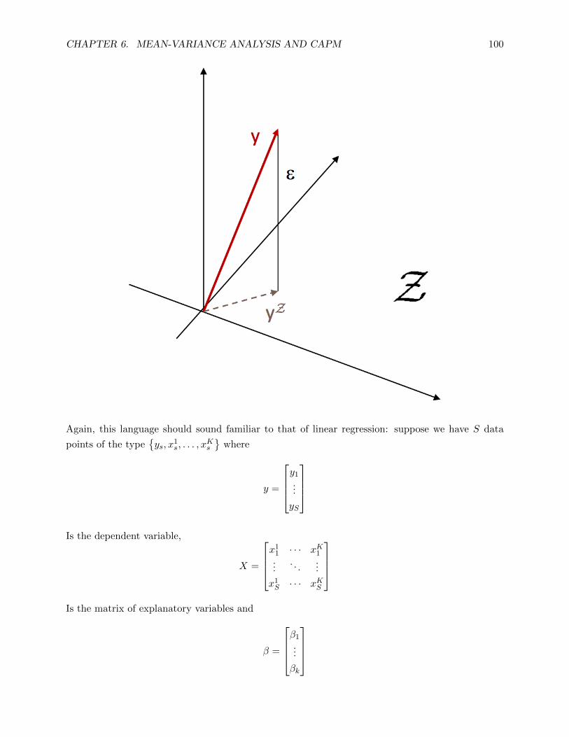
CHAPTER 6. MEAN-VARIANCE ANALYSIS AND CAPM 100
Again, this language should sound familiar to that of linear regression: suppose we have S data
points of the typeys, x
1s, . . . , x
Ks
where
y =
y1
...
yS
Is the dependent variable,
X =
x1
1 · · · xK1...
. . ....
x1S · · · xKS
Is the matrix of explanatory variables and
β =
β1
...
βk
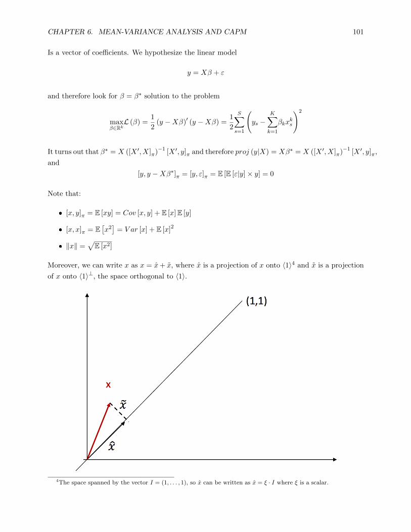
CHAPTER 6. MEAN-VARIANCE ANALYSIS AND CAPM 101
Is a vector of coefficients. We hypothesize the linear model
y = Xβ + ε
and therefore look for β = β∗ solution to the problem
maxβ∈RkL (β) =
1
2(y −Xβ)′ (y −Xβ) =
1
2
S∑s=1
(ys −
K∑k=1
βkxks
)2
It turns out that β∗ = X ([X ′, X]π)−1 [X ′, y]π and therefore proj (y|X) = Xβ∗ = X ([X ′, X]π)−1 [X ′, y]π,
and
[y, y −Xβ∗]π = [y, ε]π = E [E [ε|y]× y] = 0
Note that:
[x, y]π = E [xy] = Cov [x, y] + E [x]E [y]
[x, x]π = E[x2]
= V ar [x] + E [x]2
‖x‖ =√E [x2]
Moreover, we can write x as x = x+ x, where x is a projection of x onto 〈1〉4 and x is a projection
of x onto 〈1〉⊥, the space orthogonal to 〈1〉.
4The space spanned by the vector I = (1, . . . , 1), so x can be written as x = ξ · I where ξ is a scalar.

CHAPTER 6. MEAN-VARIANCE ANALYSIS AND CAPM 102
Moreover we have:
E [x] = [x, I]π = [x+ x, I]π = [x, I]π = [ξ · I, I]π = ξ · [I, I]π︸ ︷︷ ︸=1
= ξ constant.
V ar [x] = E[(x− E [x] · I)2
]= E
[(x+ x− E [x] · I)2
]= E
[(ξ · I + x− ξ · I)2
]= V ar [x]
σx ≡√V ar [x] = ‖x‖π
Cov [x, y] = Cov [x, y] = [x, y]π
To see the last relation, just note that
Cov [x, y] = [x, y]π − E [x]E [y] = [x, y]π + [x, y]π + [x, y]π︸ ︷︷ ︸=0
+ [x, y]π︸ ︷︷ ︸=0
− E [x]E [y]︸ ︷︷ ︸=[x,y]π
= [x, y]π
6.2.1 Pricing and Expectation Kernel
Let 〈X〉 be the space of available payoffs. We know that if there is no arbitrage and the physical
probability πs is positive, then there exists a stochastic discount factor m ∈ RS such that m > 0
and a valuation functional V such that for z ∈ RS V (z) = E [mz]. Note that the stochastic discount
factor m needs not be in the asset span. We defineed a pricing kernel as the state price vector q∗
in the asset span 〈X〉: from now on we will equivalently refer to the pricing kernel as the stochastic
discount factor m∗obtained from q∗ (that is, m∗s = q∗sπs
for all s = 1, . . . , S). Clearly, for m∗ we have
V (z) = E [m∗z] for all z ∈ RS , and if a state price vector exists, m∗ is unique. Note that for any
state price density m ∈ RS and z ∈ RS we have
E [(m−m∗) z] = 0
And because m = (m−m∗) + m∗, it follows that m∗ is the projection of m on 〈X〉. Clearly, if
markets are complete m = m∗.
We define the expectations kernel as the vector k∗ ∈ 〈X〉 such that for all z ∈ RS E [z] = E [k∗z]. If
the physical probability πs is positive the expectations kernel is unique. For any z ∈ RS we have
E [(I − k∗) z] = 0
So k∗ is the projection of I on 〈X〉. Obviously, if a bond can be replicated then k∗ = I. We are
now ready to define the mean variance frontier in terms of projections.
Definition 1: We call the mean variance frontier the set F ≡ z ∈ 〈X〉 |@z′ ∈: E [z′] = E [z] , V (z′) = V (z) and V ar [z′] < V ar [z]Definition 2: We call ε the space generated by m∗ and k∗.

CHAPTER 6. MEAN-VARIANCE ANALYSIS AND CAPM 103
We can decompose any vector z ∈ RS as z = zε + ε, where zε ∈ ε and ε⊥ε. Therefore E [ε] =
E [εk∗] = 0, V (ε) = E [εm∗] = 0 and Cov (ε, zε) = E [εzε] = 0 since zε ∈ ε and ε⊥ε. It follows that
V ar [z] = V ar [zε] + V ar [ε].
Claim: ε = F .
We call frontier returns the returns of frontier payoffs with non-zero prices. Let
Rm∗
=m∗
V (m∗)=
m∗
E (m∗ ·m∗)
Rk∗
=k∗
V (k∗)=
k∗
E (k∗)
If z ∈ F then we can write z = αm∗ + βk∗, so we can write frontie rreturns as
Rz =αV (m∗)
αV (m∗) + βV (k∗)︸ ︷︷ ︸≡λ
Rm∗
+βV (k∗)
αV (m∗) + βV (k∗)︸ ︷︷ ︸=1−λ
Rk∗
Graphically, frontier returns are payoffs with price equal to 1. Note that if k∗ = c ·m∗ for some
c ∈ R, we have Rz = Rm∗
= Rk∗. If instead k∗ 6= c ·m∗ we can re-write the expression above as
Rz = Rk∗
+ λ(Rm
∗ −Rk∗)
For which we have
E [Rz] = E[Rk∗]
+ λ(E[Rm
∗]− E
[Rk∗])
and
V ar [Rz] = V ar[Rk∗]
+ 2λCov[Rk∗, Rm
∗ −Rk∗]
+ λ2V ar[Rm
∗ −Rk∗]
The FOC with respect to λ of V ar [Rz] yields λmin = −Cov
[Rk∗,Rm
∗−Rk∗]
V ar[Rm∗−Rk∗ ], so the minimum varianc
portfolio has a return of Rmin = Rk∗
+ λmin
(Rm
∗ −Rk∗). Graphically,

CHAPTER 6. MEAN-VARIANCE ANALYSIS AND CAPM 104
If a risk-free asset exists we have k∗ = I and variance and expectation of Rz simplify to:
V ar [Rz] = λ2V ar[Rm
∗]
E [Rz] = Rf + λ(E[Rm
∗]−Rf
)= Rf ± σ (Rz)
E[Rm
∗]−Rfσ (Rm∗)
Definition 3: A return is mean-variance efficient if there is no other return with
same variance but greater expectation.
Mean variance efficient returns are frontier returns withE [Rz] ≥ E[Rmin
]. If a risk-free asset can
be replicated, we have:
1. Mean variance efficient returns correspond to returns with λ = λmin = 0
2. The portfolio with return equal to the pricing kernel is not mean variance efficient, since
E[Rm
∗]= E[m∗]
E[(m∗)2]< 1
E[m∗] = Rf , where the inequality follows from V ar [m∗] = E[(m∗)2
]−
E [m∗]2 > 0.
Now take two frontier portfolios with returns Rλ = Rk∗
+ λ(Rm
∗ −Rk∗)
and Rµ = Rk∗
+
µ(Rm
∗ −Rk∗): their covariance is given by
Cov[Rλ, Rµ
]= V ar
[Rk∗]
+ (λ+ µ)Cov[Rk∗, Rm
∗ −Rk∗]
+ λµV ar[Rm
∗ −Rk∗]

CHAPTER 6. MEAN-VARIANCE ANALYSIS AND CAPM 105
These two portfolios have zero covariance if
µ = µ0 = −V ar
[Rk∗]
+ λCov[Rk∗, Rm
∗ −Rk∗]
Cov [Rk∗ , Rm∗ −Rk∗ ] + λV ar [Rm∗ −Rk∗ ]
For all λ 6= λmin, µ0 exists and clearly µ0 = 0 is a risk-free bond can be replicated.
6.2.2 Beta Pricing
Since Rλ and Rµ are frontier returns, we can write
Rβ = Rµ + β(Rλ −Rµ
)(6.1)
Where Rβ is again a frontier return. Consider any asset with payoff xj : we know it can be decom-
posed in xj =(xj)ε
+ εj with V(xj)
= V((xj)ε)
and E[xj]
= E[(xj)ε]
since εj⊥ε. The return of(xj)ε
is
Rj =(Rj)ε
+εj
V (xj)
Where(Rj)ε
is a frontier return: using relation (1) above for(Rj)ε
we can write
Rj = Rµ + βj
(Rλ −Rµ
)+
εj
V (xj)
Taking expectations we obtain the Beta Pricing Equation
E[Rj]
= E [Rµ] + βj
(E[Rλ]− E [Rµ]
)Moreover, assuming µ = µ0,
Cov[Rλ, Rj
]= βjV ar
[Rλ]
Since Rλ⊥ εj
V (xj), or βj =
Cov[Rλ,Rj]V ar[Rλ]
.5 If a risk-free asset exists, the beta pricing equation simplifies
to
E[Rj]
= Rf + βj
(E[Rλ]−Rf
)Note the similarity with the CAPM relation: here we have Rλ (a general frontier return) instead
of the market return, which we need to identify to be able to price assets. CAPM is equivalent to
this formulation with Rλ = Rm, that is, the market portfolio is a frontier return. We can derive
the conditions under which the market portfolio is a frontier return: suppose there are two periods
t = 0, 1. Agent i has individual endowmentwi1 at time t = 1, and the aggregate endowment at t = 1
5Because Rλ ∈ F while εj⊥F .
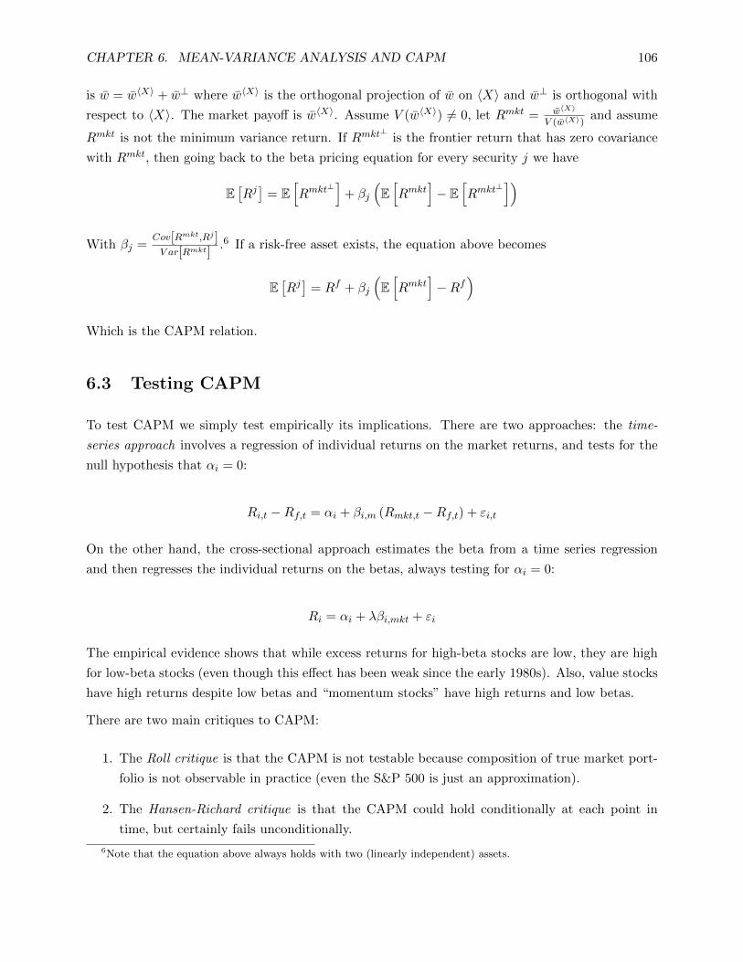
CHAPTER 6. MEAN-VARIANCE ANALYSIS AND CAPM 106
is w = w〈X〉 + w⊥ where w〈X〉 is the orthogonal projection of w on 〈X〉 and w⊥ is orthogonal with
respect to 〈X〉. The market payoff is w〈X〉. Assume V (w〈X〉) 6= 0, let Rmkt = w〈X〉
V (w〈X〉)and assume
Rmkt is not the minimum variance return. If Rmkt⊥
is the frontier return that has zero covariance
with Rmkt, then going back to the beta pricing equation for every security j we have
E[Rj]
= E[Rmkt
⊥]
+ βj
(E[Rmkt
]− E
[Rmkt
⊥])
With βj =Cov[Rmkt,Rj]V ar[Rmkt]
.6 If a risk-free asset exists, the equation above becomes
E[Rj]
= Rf + βj
(E[Rmkt
]−Rf
)Which is the CAPM relation.
6.3 Testing CAPM
To test CAPM we simply test empirically its implications. There are two approaches: the time-
series approach involves a regression of individual returns on the market returns, and tests for the
null hypothesis that αi = 0:
Ri,t −Rf,t = αi + βi,m (Rmkt,t −Rf,t) + εi,t
On the other hand, the cross-sectional approach estimates the beta from a time series regression
and then regresses the individual returns on the betas, always testing for αi = 0:
Ri = αi + λβi,mkt + εi
The empirical evidence shows that while excess returns for high-beta stocks are low, they are high
for low-beta stocks (even though this effect has been weak since the early 1980s). Also, value stocks
have high returns despite low betas and “momentum stocks” have high returns and low betas.
There are two main critiques to CAPM:
1. The Roll critique is that the CAPM is not testable because composition of true market port-
folio is not observable in practice (even the S&P 500 is just an approximation).
2. The Hansen-Richard critique is that the CAPM could hold conditionally at each point in
time, but certainly fails unconditionally.
6Note that the equation above always holds with two (linearly independent) assets.

CHAPTER 6. MEAN-VARIANCE ANALYSIS AND CAPM 107
Important counter-arguments include that the anomalies that make the CAPM fail empirically are
the result of excessive data mining, or that these anomalies are concentrated in small and illiquid
stocks, or yet that arkets are just inefficient and therefore it is impossible to test CAPM because
it already implies market efficiency. Finally, there are several practical issues in estimating the
regressions above: how do we estimate all the parameters we need for portfolio optimization? What
is the market portfolio? Should we impose any trade restrictions? What about international assets
and currency risk? Or even, should we assume a static market portfolio or one that changes over
time?
6.4 Practical Issues
An investor looking to build a mean-variance portfolio has to estimate J means (one for each asset),
J variances and J(J−1)2 covariances.
6.4.1 Estimating Means
One way of eatimating means is the following: for any partition of [0, T ] with N intervals (so that
∆t = TN ), E [R] = 1
∆t1N
N∑i=1Ri∆t = pT−p0
N (in log-prices), so knowing the first and last prices is
sufficient.
A different approach is to take the log-return on the market Xk, with k = 1, . . . , n over a period of
length h (that is, ∆ = nh ). We want to estimate the dynamics
Xk = µ ·∆ + σ ·√
∆εk
Where εkiid∼ N (0, 1). The standard estimator for µ is µ = 1
h
n∑k=1
Xk, which has mean µ and variance
σ2
h : remarkably, the accuracy of the estimator depends only upon the total length of the observation
period h and not upon the number of observations n.
6.4.2 Estimating Variances
Using an “intuitive” estimator σ2 = 1h
n∑k=1
X2k we get
E[σ2]
= σ2 + µ2 · hn
V ar[σ2]
=2σ2
n+
4 · µ2 · hn2

CHAPTER 6. MEAN-VARIANCE ANALYSIS AND CAPM 108
Clearly, this estimator is biased since we did not subtract the expected return for each realization
in the formula for σ2. The magnitude of the bias however is decreasing in n, so the accuracy can
be improved my sampling the data more frequently.
Another approach is to do as we did for the means: for any partition of [0, T ] with N intervals (so
that ∆t = TN ), E [R] = 1
∆t1N
N∑i=1ri∆t = pT−p0
N . Then we take
V ar [R] =1
N
N∑i=1
(Ri∆t − E [R])2 → σ2 as N →∞
In theory, observing the same time series at progressively higher frequencies increases the precision
of the estimate. However in practice we run into a number of issues: for instance, over shorter time
intervals increments are non-Gaussian; volatility is time-varying (so stochastic volatility, GARCH
and other more complicated models are more appropriate) and there is always market microstructure
“noise” that spoils the estimation.
6.4.3 Estimating Covariances
In theory, the estimation of covariances shares the features of variance estimation. In practice
however, it is difficult to obtain synchronously observed time-series: this may require interpolation,
which affects the covariance estimates. Moreover, the number of covariances to be estimated grows
very quickly with the number of assets, sp that the resulting covariance matrices are oftenunstable.
A possible solution is represented by “shrinkage estimators” (see Ledoitand Wolf, 2003, “Honey, I
Shrunk the Covariance Matrix”).
6.5 Unstable Portfolio Weights
A properly designed regression yields (positive) portfolio weights. There is a large literature on
statistical tests for the significance of these weights: for instance, Britton-Jones (1999) test it for
an international portfolio between 1977 and 1996 in 11 countries. The results are striking: weights
vary significantly across time and in the cross section, and standard errors on coefficients tend to
be very large.
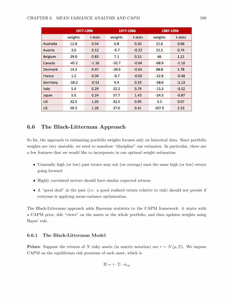
CHAPTER 6. MEAN-VARIANCE ANALYSIS AND CAPM 109
6.6 The Black-Litterman Approach
So far, the approach to estimating portfolio weights focuses only on historical data. Since portfolio
weights are very unstable, we need to somehow “discipline” our estimates. In particular, there are
a few features that we would like to incorporate in our optimal weight estimation:
Unusually high (or low) past return may not (on average) earn the same high (or low) return
going forward
Highly correlated sectors should have similar expected returns
A “good deal” in the past (i.e. a good realized return relative to risk) should not persist if
everyone is applying mean-variance optimization.
The Black-Litterman approach adds Bayesian statistics to the CAPM framework: it starts with
a CAPM prior, dds “views” on the assets or the whole portfolio, and then updates weights using
Bayes’ rule.
6.6.1 The Black-Litterman Model
Priors: Suppose the returns of N risky assets (in matrix notation) are r ∼ N (µ,Σ). We impose
CAPM on the equilibrium risk premium of each asset, which is
Π = γ · Σ · weq

CHAPTER 6. MEAN-VARIANCE ANALYSIS AND CAPM 110
Where γ is the investors’ corfficient of risk aversion and weq is the vector of equilibrium (market)
portfolio weights. The investor is assumed to start with a Bayesian prior µ = Π + εeq, where
εeq ∼ N (0, τ · Σ): the variance of the equilibrium return estimates is assumed to be proportional
to the variance of the returns (and τ is a scaling parameter).
Views: Investor views on a single asset affect many weights. Investor views regarding the perfor-
mance of K portfolios (e.g. each portfolio can contain only a single asset). Let P be a K × Nmatrix of ortfolio weights, and let Q be a K × 1 vector of views regarding the expected returns of
these portfolios. Investor views are assumed to be imprecise:
P · µ = Q+ εv
Where εv ∼ N (0,Ω). Without loss of generality, Ω is assumed to be diagonal; εeq and εv are
assumed to be independent. Recall that if X1 and X2 arenormally distributed as
(X1
X2
)∼ N
((µ1
µ2
),
(Σ11 Σ12
Σ21 Σ22
))
Then the conditional distribution is given by
X1|X2 = x ∼ N(µ1 + Σ12Σ−1
22 (x− µ2) ,Σ11 − Σ12Σ−122 Σ21
)Posterior: The Black-Litterman posterior distribution of expected returns R|Q is Gaussian with
E [R|Q] =[(τ · Σ)−1 + P ′Ω−1P
]−1 [(τ · Σ)−1 Π + P ′Ω−1Q
]V ar [R|Q] =
[(τ · Σ)−1 + P ′Ω−1P
]−1
For example, consider the 2 assets case. You have a view on the (equally weighted) portfolio12µ1 + 1
2µ2 = q + εv. Then
E [R|Q] =
[(τ · Σ)−1 +
1
2Ω
]−1 [(τ · Σ)−1 Π +
q
2Ω
]
V ar [R|Q] =
[(τ · Σ)−1 +
1
2Ω
]−1
There are several advantages to this approach. First, returns are adjusted only partially toward
the investor’s views using Bayesian updating, thus recognizing that views may be due to estimation
error and only highly precise or confident views are weighted heavily. Second, returns are modified
in a way that is consistent with economic priors: highly correlated sectors have returns modified in
the same direction. Finally, returns can be modified to reflect absolute or relative views, and the

CHAPTER 6. MEAN-VARIANCE ANALYSIS AND CAPM 111
resulting weight have reasonable values and do not load up on the estimation error.

CHAPTER 6. MEAN-VARIANCE ANALYSIS AND CAPM 112
Exercises
1) Consider an economy in which there are three risky assets (A, B, and C) and one riskless asset.
Asset A has an expected net return of 15% and the variance of its return is 0.20. Asset B has an
expected net return of 20% and a variance of 0.40. Asset C has an expected net return of 55% and
its variance is 0.60. The covariance between each pair of asset returns is zero. There are 3000 shares
of A available in the economy and the current price of A is 20. There are 1500 shares of B available
and its current price is 40. Finally, there are 10,000 shares of C outstanding and the current price
of C shares is 18. Does there exists a riskless rate of return Rf so that given the current prices of
the risky asset , the Sharpe-Lintner pricing equation E[Rj]
= Rf + βj,m(E[Rmkt
]−Rf
)? If so,
what is that rate? If not, why is it impossible to find such a rate?
2) Show as rigorously as possible that ε = F , that is, the space generated by the expectations and
pricing kernel is the mean-variance frontier. Be careful: you need to show both F ⊆ ε and ε ⊆ F .
3) A manufacturing firm has just been founded and needs to build a factory. It has a choice between
two different types of factory (factory 1 and factory 2) and the cost of building each is K1 = 120
and K2 = 50, respectively. Only one factory can be built at this time. The table below lists the
properties of the payoffs (X1 and X2) from the different projects, the gross market rate of return
(Rmkt) and the gross risk free rate (Rf ). You may assume that all the assumptions of the CAPM
hold and that the management seeks to maximize the market value of the firm at all times. To
simplify calculations, the net risk free rate of return is set to zero. You may also assume that any
investments the firm makes have a negligible effect on the market portfolio.
E [X1] = 300 E [X2] = 150 E[Rmkt
]= 1.1
V ar [X1] = 10, 000 V ar [X2] = 2, 500 V ar[Rmkt
]= 0.01
Corr [X1, X2] = 0.4 Corr[X1, R
mkt]
= 0.8 Corr[X2, R
mkt]
= 0.2
a) In a meeting, an executive argues as follows: Since the expected (net) return on factory 2 is
higher (200% vs. 150%), that one should be built. Another executive disagrees and argues that
naturally one should always build factory 1, since the expected profit is larger than if factory 2 were
built (180 vs. 100). Which (if any) of the two decision procedures suggested will maximize the firm
value? Why?
b) In the end, the executives ask you to decide which factory to build. What is your decision?
Compute the firm’s total value V . If 100 shares are outstanding, what is the stock price P?
(Assume that CAPM holds).
c) Suppose factory 2 has been built (do not assume this was the correct answer to part b)!) and
a year has passed. It is time to expand, and the firm plans to build factory 1. However, it has no
cash to fund the investment and needs to raise K1 = 120 in the capital market. The firm decides
to issue shares for a total value of 120. How many shares should it issue and at what price?

CHAPTER 6. MEAN-VARIANCE ANALYSIS AND CAPM 113
d) In a shareholder meeting, there is a heated argument about whether or not to go ahead with the
building of the factory and the stock issue. An angry shareholder claims that although expected
returns are impressive, factory 1 is an extremely risky investment, not least because most of its
risk is not diversifiable. She argues that exposing the firm to this risk will reduce the value of her
shares. A concerned executive responds by pointing out that since the values of the two factories
are negatively correlated, the project does not really increase the riskiness of the firm’s portfolio of
assets that much and is therefore a good investment. What, in your opinion, is missing from the
analysis by the shareholder and the executive? Are their arguments valid?
4) Assume that the market return is in the mean variance frontier. Suppose that there are three
equally likely states. One security is risk free and has a gross return Rf = 0.9. A second security
has a gross return vector of (0, 1, 1). The market portfolio has a payoff of (1, 2, 2).
a) Use the CAPM to price a security that pays off (0, 0, 1).
b) Find the expectations kernel and pricing kernel.
c) Calculate the price of the same security (that pays off (0, 0, 1)) using the pricing kernel.
5) Show that E[σ2]
= σ2 + µ2 · hn and V ar[σ2]
= 2σ2
n + 4·µ2·hn2 .
6) Derive the expressions for the mean and variance of the Black-Litterman posterior distribution
of expected returns R|Q.

Chapter 7
The Multi-Period Model
How can we deal with a multi-period setup in which several outcomes are possible after each outcome
realizes? One way to tackle this problem is to bring down the problem to a set of many “smaller”
one-period model problems:
114

CHAPTER 7. THE MULTI-PERIOD MODEL 115
With this approach however, we need a more efficient way to define and work with the information
available at each time step. A natural way to approach this is using the concept of algebra:
7.1 Model Setup
We begin by defining an algebra:
Definition 1: Given a state space Ω, an algebra F is a non-empty collection of
subsets of Ω such that 1) Ø ∈ F 2) A ∈ F ⇒ AC ∈ F 3) A,B ∈ F ⇒ A ∪B ∈ F .
Definition 2: A random variable Y is measurable with respect to the algebra F if
ω ∈ Ω|Y (ω) ≤ y ∈ F for all y ∈ R.
Definition 3: A stochastic process is a collection of random variables YtTt=0.
Definition 4: A filtration is a collection of algebras FT = FsTs=t such that if u ≤ vthen Fu ⊆ Fv.
Definition 5: A stochastic process YtTt=0 is adapted to the filtration FT = FsTs=tif Ys is measurable with respect to Fs for s = t, . . . , T .
Adaptation is the requirement that people cannot see in the future. Moving from a static to a
dynamic setting, we need to adapt our notation:

CHAPTER 7. THE MULTI-PERIOD MODEL 116
Rather than asset holdings, we will talk about dynamic strategies
Instead of asset payoff vectors x we will talk about the “next period payoff” xt+1 + pt+1 of a
strategy
Instead of the asset span, we will talk about the subset of marketed dynamic strategies
Market completeness can be interpreted in two ways: static completeness (Debreu complete-
ness) and dynamic completeness (Arrow completeness)
We defined no arbitrage with respect to asset holdings, but now it will be defined on dynamic
strategies
States s ∈ s1, s2, . . . sS generalize to events At,i and final states st,i
State prices qs become event prices qt,i
The risk-free rate Rft varies over time
the discount factor ρt is time-dependent and discounts from t to 0
The risk-neutral probability is πQ (At,i) =qt,iρt
The pricing kernel now reads Mtpjt = Et
[Mt+1
(pjt+1 + xjt+1
)], and Mt = Rft+1Et [Mt+1]
We will use trees to illustrate dynamics. In the picture below, the tree has 7 events. Every event has
a positive probability attached to it, and we impose the consistency requirement that the probability
of any event equals the sum of the events that follow from its node: for example, denoting πt,s the
probability of At,s, we have π1,1 = π2,1 + π2,2. Clearly, for each t we have∑sπt,s = 1.

CHAPTER 7. THE MULTI-PERIOD MODEL 117
There are two ways to reduce this seemingly more complicated model to the one-period model.
The first is to boil down every event to a final state, and apply what we know from the one-period
model:
Note that if we simplify the tree in this way it follows that to achieve completeness we will need six
independent assets, one for each final state. The second way is to reduce each branch of the tree to
a one-period model:
In this case, assets can be re-traded conditionally on the the occurrence of event A1,1 or A1,2.
Completion can be achieved with two categories of assets: short-lived assets pay off only in the
period following the one in which they are traded, while long-lived assets pay off over many periods.
CHAPTER 7. THE MULTI-PERIOD MODEL 118
7.2 Dynamic Trading and Market Completeness
Suppose now that asset can be traded in each period. This allows for dynamic completion, as well
as for the existence of bubbles and ponzi schemes in an infinite horizon setting. We will study
completeness with both short- and long-lived assets.
A short-lived asset is an asset that pays out only in the period immediately after the asset is issued.
Without uncertainty and with T one-period assets (that is, T assets that can be bought in period
t − 1 at price pt and pays off in period t for t = 1, . . . , T ), completeness requires that we are able
to transfer wealth between ant two periods. For example, if zero coupon bonds are traded in each
period and T = 2, at time t = 0 we can buy a quantity p2 of bonds that pay off at time t = 1 at a
total cost of p1p2, and then in period t = 1 we can invest the proceeds from the bond we bought to
buy one unit of the bond that pays at time t = 2: in this way we replicated a bond that is bought at
t = 0 and pays $1 at time t = 2, and therefore markets are complete. In general, for T periods the
cost of rolling over this kind of short-lived bond strategy is just pt ·pt+1 · . . . ·pT−1, and completeness
requires that we are able to transfer wealth between any two periods t and t′ (not just consecutive).
With uncertainty the reasoning is very similar. Suppose the event tree is as follows:
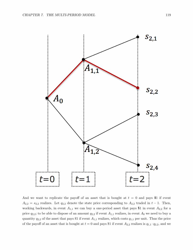
CHAPTER 7. THE MULTI-PERIOD MODEL 119
And we want to replicate the payoff of an asset that is bought at t = 0 and pays $1 if event
A2,2 = s2,2 realizes. Let q2,2 denote the state price corresponding to A2,2 traded in t − 1. Then,
working backwards, in event A1,1 we can buy a one-period asset that pays $1 in event A2,2 for a
price q2,2; to be able to dispose of an amount q2,2 if event A1,1 realizes, in event A0 we need to buy a
quantity q2,2 of the asset that pays $1 if event A1,1 realizes, which costs q1,1 per unit. Thus the price
of the payoff of an asset that is bought at t = 0 and pays $1 if event A2,2 realizes is q1,1 ·q2,2, and we

CHAPTER 7. THE MULTI-PERIOD MODEL 120
can repeat the argument for all other events to see that this market achieves dynamic completeness.
With long-lived assets, consider a T -period model without uncertainty. There is a single asset
paying $1 in t = T , which is tradable in each period for a price pt: this means that sequentially,
there are T prices for this asset. The payoff can be transferred from period s to period t > s by
purchasing the asset at time s and selling it in period t. For example, suppose there are two assets
that pay off like in the graph below.
The assets are long-lived, since they can be re-traded at t = 1 for the price pjt,s. Note that we have
two assets, but each assets can be traded in three events; moreover, the price of each asset can be
endogenously determined at time t = 0. Although one may be tempted to think that because we
only have 2 assets markets cannot be complete, in fact dynamic trading provides a way to transfer
wealth in all events:

CHAPTER 7. THE MULTI-PERIOD MODEL 121
Call trading strategy [j, At,i] the cash flow of asset j that is purchased in eventAt,i and sold one period
later. There are six such trading strategies: [1, A0], [1, A1,1], [1, A1,2], [2, A0], [2, A1,1], [2, A1,2]. For
example, trading strategy [1, A1,1] costs p11,1 and pays out $1 in the first final state and zero in all
other events; and trading strategy [1, A0] costs p10 and pays out p1
1,1 in event 1, p11,2 in event 2, and
zero in all the final states.
These six trading strategies give rise to a 6× 6 payoff matrix:
Strategy [1, A0] [2, A0] [1, A1,1] [2, A1,1] [1, A1,2] [2, A1,2]
Event A0 −p10 −p2
0 0 0 0 0
Event A1,1 p11,1 p2
1,1 −p11,1 −p2
1,1 0 0
Event A1,2 p11,2 p2
1,2 0 0 −p11,2 −p2
1,2
State s2,1 0 0 1 0 0 0
State s2,2 0 0 0 1 0 0
State s2,3 0 0 0 0 1 0
State s2,4 0 0 0 0 0 1
The payoff matrix is regular (and hence markets are complete) if and only if the submatrix
p11,1 p2
1,1
p11,2 p2
1,2
Is regular (that is, it has rank equal to 2). The components of this submatrix are the prices of the
two assets conditional on period-1 events. There are cases in which these are collinear in equilibrium:

CHAPTER 7. THE MULTI-PERIOD MODEL 122
for instance when the per capita endowment is the same in event A1,1 and A1,2, in state s2,1 and
s2,3, and in state s2,2 and s2,4, and if the probability of reaching state s1,1 after event A1,1 is the
same as the probability of reaching state s2,3 after event A1,2 then the submatrix is singular (but,
one might argue, then events A1,1 and A1,2 are effectively equivalent and could be collapsed into a
single event). Moreover, a random square matrix is regular: this means that generically, the market
is dynamically complete (that is, it is not complete only for information trees and asset structures
which have zero probability of showing up in any application).
We call branching number the maximum number of branches that fan out from any event in the
uncertainty tree: it turns out that this is also the number of assets necessary to achieve dynamic
completeness. This generalizes to the continuum of events and continuous time case, in which a
small number of assets is sufficient to achieve completeness because the need for many assets to
achieve completeness that arises from a large number of possible events is offset by the ability to
trade continuously, thus generating a large number of trading strategies. The classic example is the
Black-Scholes formula: Cox, Ross and Rubinstein showed that is is possible to build a binomial tree
model of Black-Scholes, with constant interest rates and in which the stock can only go up or down,
in which the market is dynamically complete with just two assets: the stock and the risk-free bond.
Thus an option on the stock can be replicated with dynamic delta-hedging.
7.3 The Multi-Period Stochastic Discount Factor
The idea of no arbitrage extends naturally to the multi-period setting: an arbitrage is a strategy
that has either no cost today but some positive payoff along the tree or a negative cost today and
no negative payoff along the tree. Moreover, it is equivalent to having no static arbitrage in each
branch of the tree.
Recall that no arbitrage requires that there esxists a positive stochastic discount factor mt+1 for
each subperiod t such that
pt = Et [mt+1 (pt+1 + xt+1)]
Define the multi-period stochastic discount factor as1
Mt+1 = m1 ·m2 · . . . ·mt+1
Multiplying each side by m1 ·m2 · . . . ·mt (which is measurable until the time t filtration) we get
Mtpt = Et [Mt+1 (pt+1 + xt+1)]
Assuming for this asset there is a stream of cash flows xt∞t=1 where each xt is a random payoff,
1We assume m0 = 1 from now on.
CHAPTER 7. THE MULTI-PERIOD MODEL 123
we have for time t = 0
p0 = E0 [M1 (p1 + x1)]
similarly
M1p1 = E1 [M2 (p2 + x2)]
plugging in the equation for p0 we have
p0 = E0 [E1 [M2 (p2 + x2)] +M1x1] = E0 [E1 [M2p2 +M2x2 +M1x1]]
The Law of Iterated Expectations (LIE) states that, because of the property of filtrations that if
u ≤ v then Fu ⊆ Fv, for any random variable X the time-u expectation of the random variable
“time-v expectation of X” is equal to the time-u expectation of X. The intuition is as follows:
consider your current guess of what the weather will be on sunday, and compare it to the guess that
you will have on saturday about the weather on sunday. LIE states that your current guess on your
guess for the sunday weather is the same as your current guess for the sunday weather. Therefore
we get
p0 = E0 [M2p2 +M2x2 +M1x1]
Iterating k steps forward we have
p0 = E0 [Mkpk] +k∑t=1
E0 [Mtxt]
Taking the limit for k →∞ (and assuming limk→∞
E0 [Mkpk] = 0) we have
p0 =∞∑t=1
E0 [Mtxt]
In terms of projections, recall that m∗t+1 = proj (mt+1| 〈Xt+1〉), that is, there exists some h∗t such
that m∗t+1 = Xt+1h∗t and
pt = Et[X′t+1m
∗t+1
]= Et
[X′t+1Xt+1
]h∗t
So that
h∗t =(Et[X′t+1Xt+1
])−1pt
And therefore
m∗t+1 = Xt+1
(Et[X′t+1Xt+1
])−1pt
Clearly we also have M∗t ≡ m∗1 ·m∗2 · . . . ·m∗t ∈ 〈Xt〉. Further, we can express m∗t+1 in terms of the

CHAPTER 7. THE MULTI-PERIOD MODEL 124
covariance of returns Σt:
m∗t+1 = Et[m∗t+1
]+[pt − Et
[m∗t+1
]Et [Xt+1]
]′Σ−1t [Xt+1 − Et [Xt+1]]
Ans also in terms of covariance of excess returns Ψt ≡ Covt[Ret+1
]:
m∗t+1 =1
Rft− 1
RftEt[Ret+1
]′Ψ−1t
[Ret+1 − Et
[Ret+1
]]Compare it to its continuous-time analogous2
dm∗tmt
= −rfdt−(µ+
D
p− rf
)′Ψ−1t dZt
Recall that if the one-period stochastic discount factor mt is not time-varying (that is, the distribu-
tion of mt is i.i.d for each t), then the expectations hypothesis holds and the investment opportunity
set does not vary. The corresponding R∗t of a single-factor state-price beta model is then relatively
easy to estimate, since over time we collect more and more realizations of R∗t . However, if mt (or
the correspondingR∗t ) is time-varying, then we can assume that it depends on some state variable
and need a multi-factor model to account for it. Indeed, suppose that R∗t = R∗ (zt), where zt is
some state variable. For example, suppose that zt can be either 1 or 2 with equal probability. Then
we could take all the periods in which zt = 1 and back out R∗ (1), and find R∗ (2) in a similar way.
Is it possible to do so in reality? The answer is no, because we have hedges across state variables.
7.4 Martingales
Let Xt be a stochastic process and xt a sequence of its realizations. We say that Xt is a
martingale if E [Xt+1|Xt = xt, Xt−1 = xt−1, . . . , X1 = x1] = xt. Paul Samuelson argued in 1965 that
asset prices have to be martingales in equilibrium:
pt =1
1 + rftEQt [pt+1 + dt+1]
this is trivial assuming assuming no dividends, no discounting and risk-neutral agents. Let’s examine
these cases one by one.
With discounting, in order for the price process to follow a martingale we simply need:
Et [δpt+1] = pt
With dividend payments, things are more complicated because pt depends on the dividend of the
2Where Zt is a Brownian Motion.

CHAPTER 7. THE MULTI-PERIOD MODEL 125
asset in period t+ 1 but pt+1 does not (it is the ex-dividend price). However, for example, the value
of a fund that keeps reinvesting the dividends follows a martingale (LeRoy 1989): suppose the fund
owns nothing but one unit of asset j. Assuming agents are risk-neutral, the value of the fund at
time 0 is
f0 = p0 = E
∑t≥1
δtxjt
= δE[p1 + xj1
]
After receiving a (state contingent) dividend xj1, the fund buys more of asset j at price p1, thus
owning 1 +xj1p1
units of the asset. The expected discounted value of the fund is then
E [f1] = E
[δp1
(1 +
xj1p1
)]= E
[δ(p1 + xj1
)]= p0 = f0
So the discounted expected value of the fund is a martingale.
A similar statement is true of the agent is risk-averse. The difference is that we have to discount with
the risk-free interest rate instead of the agent’s discount factor, and use risk-neutral probabilities
(by now you should have an idea about why it is also called “equivalent martingale”) instead of
objective probabilities. Just like in the one-period model, we define the risk-neutral probability of
event A as
πQ (At,s) =πt,sMt,s
ρt
Where ρt =
(t∏
s=0Rfs
)−1
is the risk-free discount factor between 0 and t. The initial value of the
fund is
f0 = p0 = E
∑t≥1
Mtxjt
= E
M1xj1 +
∑t≥2
Mtxjt
= E
m1
xj1 +∑t≥2
t∏s=2
mtxjt
=
= E[m1
(xj1 + p1
)]= E
[M1
(xj1 + p1
)]Under the risk-neutral measure, this can be rewritten as
f0 = ρ1EQ[xj1 + p1
]= ρ1EQ [f1]
Therefore, the properly discounted (ρ instead of δ) and properly expected (πQ instead of π) value
of the fund is indeed a martingale.
We can now introduce a fifth asset pricing formula. Let Ps (t, T ) be the time-s price of a (zero-
coupon) bond to be purchased at time t and with maturity T . We know the pricing relation is
Pt (t, T ) = Et [mt+1Pt+1 (t+ 1, T )]

CHAPTER 7. THE MULTI-PERIOD MODEL 126
Dividing side by side the pricing relation for a generic asset j and rearranging we get
pjtPt (t, T )
= Et
Pt+1 (t+ 1, T )mt+1
(xjt+1 + pjt+1
)Pt+1 (t+ 1, T )Et [mt+1Pt+1 (t+ 1, T )]
= EFTt
[xjt+1 + pjt+1
Pt+1 (t+ 1, T )
]
Where the expectation is taken with respect to the risk-forward measure FT for which πFTs =
πsPt+1(t+1,T )mt+1
Et[mt+1Pt+1(t+1,T )] (note that πFTs ≥ 0 andS∑s=1
πFTs = 1 guarantee that πFT is a probability distribu-
tion). This asset pricing formula was speficically devised to price bond options, and boils down to
the risk-neutral measure if t+ 1 = T like in the one-period model case.
7.5 Ponzi Schemes and Rational Bubbles
Allowing for an infinite horizon allows agents to borrow an arbitrarily large amount and roll over
debt forever, without ever repaying the debt. This is referred to as a Ponzi scheme: it allows
infinite consumption. Consider a model with infinite horizon, no uncertainty and a complete set of
short-lived bonds. Let zt be the amount of bonds in the portfolio maturing in period t, and let pt be
the price of one such bond in period t− 1 (just like before). The consumption path with ct = yt + 1
is feasible: note that the agent consumes more than his endowment in each period, forever! This
can be financed with increasing debt:
zt+1 =zt − 1
pt+1
For all t ≥ 0 and z0 = 0. However, Ponzi schemes can never be part of an equilibrium because
they remove the existence of a utility maximum, since the choice set of the agent is unbounded.
Therefore we need an additional constraint, called transversality condition:
limt→∞
ptzt ≥ 0
Which implies that the value of debt cannot diverge to infinity, or equivalently, that all debt must
eventually be redeemed. There are also additional solutions to this problem that incorporate a
“bubble” component to the asset price: consider again a model with no uncertainty and a consol
delivering $1 in each period, forever. Our formula states that
ptMt = Et [Mt+1 (pt+1 + xt+1)]
In our case xt ≡ 1 and we have no uncertainty, so we can write
Mtpt = Et [Mt+1pt+1] + Et [Mt+1xt+1]
Solving forward we obtain
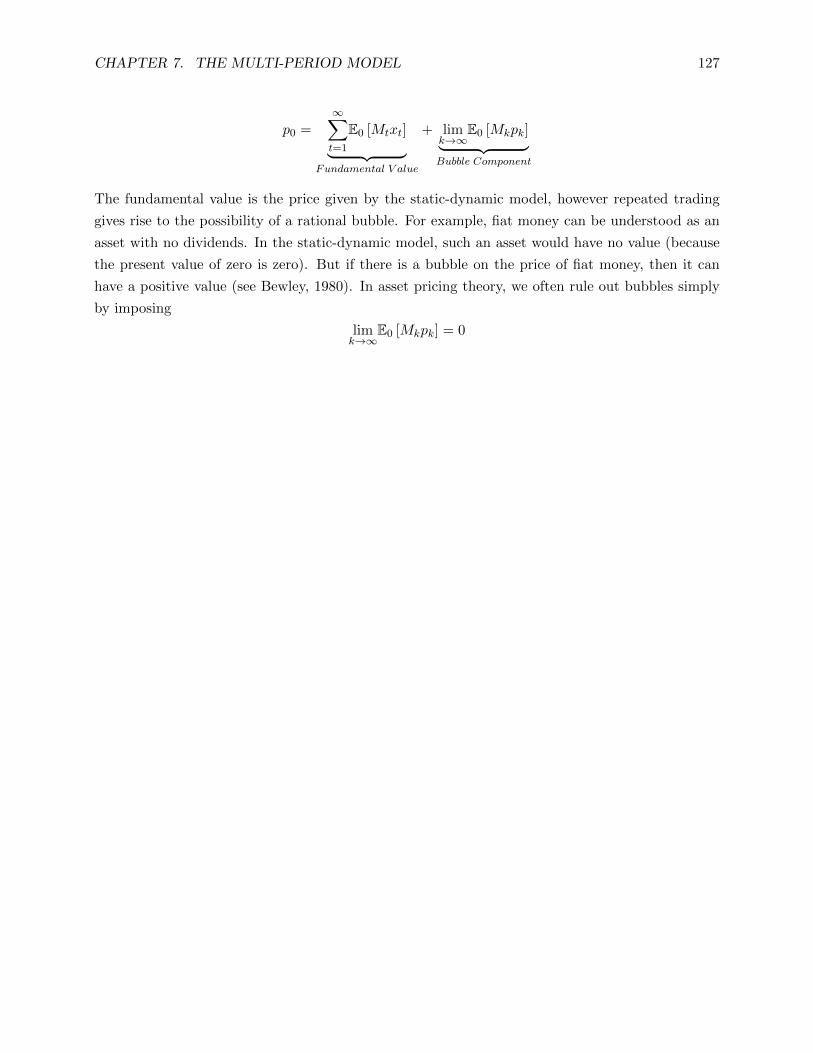
CHAPTER 7. THE MULTI-PERIOD MODEL 127
p0 =∞∑t=1
E0 [Mtxt]︸ ︷︷ ︸Fundamental V alue
+ limk→∞
E0 [Mkpk]︸ ︷︷ ︸Bubble Component
The fundamental value is the price given by the static-dynamic model, however repeated trading
gives rise to the possibility of a rational bubble. For example, fiat money can be understood as an
asset with no dividends. In the static-dynamic model, such an asset would have no value (because
the present value of zero is zero). But if there is a bubble on the price of fiat money, then it can
have a positive value (see Bewley, 1980). In asset pricing theory, we often rule out bubbles simply
by imposing
limk→∞
E0 [Mkpk] = 0

CHAPTER 7. THE MULTI-PERIOD MODEL 128
Exercises
1) Consider the following stochastic processes for a risk free bond
6.60 1.10
3.30 1.10
5.00 1.20
3.50 1.20
p1u
p1d
p0
1.00
1.00
1.00
Note that no asset pays dividends. The price of the one-period risk-free bond is normalized to 1
in each period. Suppose that the risk-neutral probability of an “up” tick is 1/3 and that of a
“down” is 2/3, for every point in time.
a) Is the market statically complete? Is the market dynamically complete?
b) What is the event price of the event up, up and of the event of only one up, ie, up, up∪up,
down?
Now suppose we change the processes in the following manner:

CHAPTER 7. THE MULTI-PERIOD MODEL 129
6.60 1.10
3.30 1.10
5.00 1.00
3.50 1.00
p1u
p1d
p0
1.00
1.00
1.00
c) Is the market statically complete? Is the market dynamically complete?
2) Consider a security market model with three dates, t = 0, 1, 2 and five states of the world,
s = 1, ..., 5. Investors have no information at time 0 and full information at time 2. At the
intermediate date, their information partition consists of the two sets A = 1, 2, 3 and B = 4, 5.There are two assets with the following price and dividend process:
p10 = 3, p1
1(A) = 3/2, p11(B) = 3;
d11(A) = 3/2, d1
1(B) = 2, d12(s) = s;
p20 = 9/4, p2
1(A) = 3, p21(B) = 6/5;
d21(A) = 1, d2
1(B) = 4/5, d22(s) = 6− s.
a) Is this price-dividend system arbitrage-free?
b) Is the contingent claim with the safe payoff stream yt = 1 (t = 1, 2) attainable? If it is, calculate
its arbitrage price and a replicating portfolio strategy.
3) Consider a security market with three dates, t = 0, 1, 2, and five states of the world, s = 1, . . . , 5.
The information structure is described by the following sequence of partitions of the state space:
P0 = 1, . . . , 5
P1 = A,B,C
P2 = 1, 2, 3, 4, 5

CHAPTER 7. THE MULTI-PERIOD MODEL 130
where A = 1, 2, B = 3, 4 and C = 5. There are four securities with terminal payoffs given
by the matrix
D =
2 4 5 1
1 1 2 1
3 2 4 1
4 5 7 1
5 6 10 1
with the j-th column corresponding to the j-th security. The prices of these securities at date
t = 0, 1 are given by 3.6 4 6.6 1
1.5 2.5 3.5 1
3.25 2.75 4.75 1
5 6 10 1
where the j-th column lists the price of the j-th security at date 0, event A, event B and event C,
respectively. The securities do not pay dividends prior to the terminal date
1. Verify that this securities market permits no arbitrage.
2. Is the market dynamically complete?
3. Compute the initial no-arbitrage price of the following three securities:
(a) A call option on security 1 with an exercise price of 3.5.
(b) A down-and-under call option on security 1 with an exercise price of 3.5. This is a call
option with an extra provision - if the price of security 1 ever drops below the exercise
price, then the option becomes worthless.
(c) A convertible security that in each state pays at the terminal date the largest payout of
the securities 1-4 in that state.

Chapter 8
Multi-Period Model: Options
Consider a European call option with strike K and maturity T . Its payoff is (ST −K)+, with no
cash flows between t = 0 and t = T . Unfortunately we are unable to statically replicate this payoff
using just the stock a risk-free bond: we need to dynamically hedge: that is, we need to engage in
a strategy where the required stock (and bond) position changes for each period, until maturity.
Since the replication strategy depends on specified random process of stock price, we need to impose
a specific model for the evolution of the stock. In a discrete time setting, the canonical model is
the Cox-Ross-Rubinstein binomial model. We assume that:
The stock pays no dividends.
The length of a period is h and over each period we assume that the stock can either go up
to St+h = u× St, or down to St+h = d× St, so for each period t the distribution is binomial.
The gross risk-free rate between periods is Rf = erf ·h, and by no arbitrage we require d <
Rf < u.
We start with a one-period binomial tree (for h = 1):
131

CHAPTER 8. MULTI-PERIOD MODEL: OPTIONS 132
Suppose we buy (“go long” in trading jargon) ∆ stocks and B bonds. The payoff from portfolio
C0 = ∆S0 +B is
C1 = ∆S1 +B ·Rf =
∆uS0 +B ·Rf if the stock goes up
∆dS0 +B ·Rf if the stock goes down
Call Cu the option payoff in the “up” state and Cd the option payoff in the “down” state. The
replicating strategy must satisfy
Cu = ∆uS0 +B ·Rf
Cd = ∆dS0 +B ·Rf
Solving for ∆ and B we get
∆ =Cu − CdS0 (u− d)
B =uCd − dCuRf (u− d)
∆ can be interpreted as the sensitivity of call price to a change in the stock price, or equivalently,
how much of the stock we should hold to hedge the option: for instance, to hedge a long call position
we need to sell ∆ units of the stock. Substituting ∆ and B in C0 we get
C0 =Cu − CdS0 (u− d)
S0 +uCd − dCuRf (u− d)
=1
Rf
[R− du− d
Cu +u−Ru− d
Cd
]
Define πQ ≡ Rf−du−d and note that u−Rf
u−d = 1− πQ:
C0 =1
Rf
[πQCu +
(1− πQ
)Cd
]=
1
RfEQ [C1]
Therefore the option price is the discounted payoff of the option under the equivalent martingale
(risk-neutral) measure Q. Note that Q is also the probability distribution that would justify the
current stock price in a risk-neutral world:
S0 =1
Rf
[πQS0u+
(1− πQ
)S0d]
Note how we never even mentioned the physical probability measure π, since we are working with
relative asset pricing.

CHAPTER 8. MULTI-PERIOD MODEL: OPTIONS 133
8.1 Two-Period Binomial Tree
A Two-Period Binomial Tree is just a concatenation of single-period binomial trees:
To price the option at time t = 0 we just apply the same procedure backwards, starting from the
two sub-trees in the final period. To summarize,
1. We compute the risk-neutral probability πQ from the stock price
2. We plug these probabilities in the formula for C at the final two nodes, and once we find the
option prices for each of the two possible states in time t = 1 we repeat the procedure for the
initial node
3. We find ∆ and B at each time to find the replicating strategy.

CHAPTER 8. MULTI-PERIOD MODEL: OPTIONS 134
The general procedure for a two-period tree is illustrated below (from now on, let p = πQ):
Suppose we observe an option price on the market of $36, while the cost of the dynamic replication
strategy is $34.08: then e can take advantage of this arbitrage opportunity by selling the option and
buying the synthetic portfolio. Today we pocket $1.92, and at maturity our cash outflows equal our
inflows.
8.2 The Relation with the Black-Scholes Model
The Black-Scholes option pricing model introduced in chapter 1 can be viewed as the limit of a
binomial tree, in which the mumber of periods n (and therefore of states) goes to infinity. To see
this, take u = eσ√Tn , d = 1
u = e−σ√Tn and Rf = er
f ·Tn where T is the time to expiration and σ
is the annualized standard deviation of the stock log-returns. The general binomial formula for a
European call on non-dividend paying stock n periods from expiration is:
C0 =1
Rf
n∑j=0
n!
j! (n− j)!pj (1− p)n−j
(ujdn−jS −K
)+Plugging in u, d and Rf and taking the limit as n→∞ we get
S0N
ln S0K +
(rf + σ2
2
)T
σ√T
−Ke−rTN ln S0
K +(rf − σ2
2
)T
σ√T

CHAPTER 8. MULTI-PERIOD MODEL: OPTIONS 135
Let d1 =lnS0K
+(rf+σ2
2
)T
σ√T
and d2 = d1 − σ2
√T , we can interpret the trading strategy under the
Black-Scholes formula as ∆ = N (d1) ∈ [0, 1] and B = −Ke−rTN (d2). We can also find the price
of a put option: by put-call parity, we have
P0 = C0 − S0 −Ke−rfT = Ke−r
fTN (−d2)− S0N (−d1)
Note that the put option has ∆ = −N (−d1) ∈ [−1, 0]
We call intrinsic value of the option the quantity (St −K)+ and time value of the option the
quantity Ct − (St −K)+:
8.3 Delta-Hedging
A stock has a delta equal to one, while a portfolio of J assets - where each asset j has notional
amount Nj - has a delta 4p =J∑j=1
∆jNj . We say that the portfolio is delta neutral if ∆p = 0. Delta-
hedging a portfolio is only a “perfect” hedge (yielding the same final payoff as the corresponding
option) with continuous trading: computing the delta is a linear approximation to the option value,
but the option price is convex and therefore the second- ahd higher-order derivatives matter. Delta-
hedging when trading is not continuous is effective only for smal price changes. Delta-Gamma
hedging reduces this convexity risk, and involves trading with other options.
CHAPTER 8. MULTI-PERIOD MODEL: OPTIONS 136
8.4 The Volatility Smile
The Black-Scholes model assumes that the volatility σ is constant over time and through strikes.
This turns out to be a bad assumption: suppose we take option prices as they are observed in the
market, and then back out the volatility implied by these prices for many values of the time to
maturity T and strike K. It turns out that the volatility implied by options on the market exhibits
a volatility “smile”, while the Black-Scholes model implies a constant parameter σ in the (T,K)
space. Interestingly, this effect was almost absent before the 1987 “Black Monday” stock market
crash, and became very evident afterwards. This means that the Black-Scholes mdoel underprices
out of the money puts (and thus in the money calls) and overprices out of the money calls (and
thus in the money puts).
One way to get around this problem is to use a different model for the volatility of the stock called
“stochastic volatility”. Other issues in the Black-Scholes include stochastic interest rates, bid-ask
spreads, other transaction costs, etc.
8.5 Collateralized Debt Obligations
Collateralized Debt Obligations (CDOs) are derivatives which repackage cash-flows from a set of
assets. Payoffs are divided in tranches: in the event of underperformance of the underlying assets,
the Senior tranche is paid out first, the Mezzanine second, and the Junior tranche last. Option
theory is very useful in pricing CDOs: the tranches can be priced using analogues from option
pricing formulas, and it is possible to estimate the “implied default correlations” between the
underlying assets that correctly price the tranches.

CHAPTER 8. MULTI-PERIOD MODEL: OPTIONS 137
Exercises
1) Consider the binomial model with u = 1.2, d = 0.9, R = 1.1 and initial asset price S = 100.
1. Calculate the price of a call option with exercise price K = 100 and n = 4 periods left until
expiry.
2. Calculate the prices of the European and American put options with the same exercise price
and time to expiry as in (a).
3. Calculate the price of an option which, at the end of the third period, gives its holder the right
to purchase the underlying asset at the minimum price realized over the life of the option.
2) A stock price is currently $30. During each 2-month period for the next 6 month it will increase
by 8% or reduce by 10%. The annual risk-free interest rate is 5% (continuous compounding).
Use a three-step tree to calculate the value of a derivative (called turbo option) that pays off
ST × (30− ST )+, where ST is the stock price in 6 months.

Chapter 9
Multi-Period Model: Fixed Income
In this chapter we will cover the basic fixed income tools in the multi-period model introduced in
the last chapter. Let us begin with the U.S. Treasuries, these include:
T-Bills, with maturity less than one year, usually with no coupon payments, and are usually
sold “at discount”, that is, the price is lower than the face value.
T-Notes (1-10 year maturity) and T-Bonds (10-30 year maturity) pay a semiannual coupon
and sell “at par”, that is, when they are issued the price is the same as the face value.
Let rt (t1, t2) denote the (annualized) interest rate from t1 to t2 prevailing at time t, and let Pt (t1, t2)
be the price of a bond quoted at t to be purchased at time t1 and maturing at t2. We call yield to
maturity the percentage increase in dollars earned from the bond (annualized). It follows that at
time t = 0 the price of a zero-coupon bond (ZCB) purchased at the same time and with maturity t
is
P0 (0, T ) =1
(1 + r0 (0, t))t
The yield curve is a plot of yields of zero coupon bonds as a function of their maturity. Usually,
long-term bond yields are higher than short-term bond yields – in which case we say that the yield
curve is upward sloping – but sometimes short-term bond yields are higher than long-term bond
yields – which we would call a downward sloping or inverted yield curve. The yield curve sometimes
has humps or other shapes as well. Formally we can represent the yield curve as the annualized
bond yield r0 (0, t) ≡ yt as a function of time. We can determine the forward rate r0 (t1, t2) as
follows: suppose you buy a ZCB with maturity t1, and at maturity you use all the proceeds from
this purchase to buy a bond with maturity t2. By no arbitrage, this strategy must have the same
price as buying a ZCB at time t = 0 with maturity t = t2:
P0 (0, t2) = P0 (0, t1)× P0 (0, t2)
138

CHAPTER 9. MULTI-PERIOD MODEL: FIXED INCOME 139
Which can be rewritten as
(1 + r0 (0, t1))t1 (1 + r0 (t1, t2))t2−t1 = (1 + r0 (0, t2))t2
Solving for the forwatd rate r0 (t1, t2),
r0 (t1, t2) =
[(1 + r0 (0, t2))t2
(1 + r0 (0, t1))t1
] 1t2−t1
− 1 =
(P0 (0, t1)
P0 (0, t2)
) 1t2−t1
− 1
A coupon bond can be similarly decomposed in the sum of n + 1 ZCBs: suppose the (annualized)
coupon payment is c and the bond pays a coupon on each date T1, . . . , Tn (with Ti − Ti−1 = 12
since coupon bonds usually pay semi-annually):
Bt (t, Tn) =
n∑i=1
c
2× Pt (t, Ti) + Pt (t, Tn)
Note that in order for the bond to sell at par, i.e. Bt (t, Tn) = 1, it must be that c = 2× 1−Pt(t,Tn)n∑i=1
Pt(t,Ti).
Finally, we can also write
Bt (t, Tn) =n∑i=1
c
2× 1
(1 + rt (t, Ti))Ti−t
+1
(1 + rt (t, Tn))Tn−t
We define the yield to maturity of a coupon bond as the y ∈ R+ that solves
Bt (t, Tn) =n∑i=1
c
2× 1
(1 + y)Ti−t+
1
(1 + y)Tn−t

CHAPTER 9. MULTI-PERIOD MODEL: FIXED INCOME 140
9.1 Duration
Duration is the sensitivity of a bond’s price to changes in interest rates. It is sometimes interpreted
as the “average time” it takes to get the money back (although this is not exactly correct). It is
defined as
D(y) = −dB(y)
dy
Where y is the bond’s yield to maturity. Let Xt be the amount the coupon bond pays at date t,
then we can write
Bt (t, Tn) =n∑i=1
XTi
(1 + y)Ti−t
And therefore the duration is equal to
D(y) = − 1
(1 + y)×
n∑i=1
(Ti − t)XTi
(1 + y)Ti−t
An alternative form of the duration is the Macaulay duration, defined as
MD (y) = −dB(y)/B (y)
dy/ (1 + y)=
(1 + y)
B (y)D (y)
Which for a coupon bond is equal to
MD (y) =1
B (y)
n∑i=1
(Ti − t)XTi
(1 + y)Ti−t
Duration is useful in the context of portfolio immunization: suppose we own a bond with maturity
t1 and we wish to trade a quantity N of a bond ith maturity t2 so that the total duration of the
portfolio is zero. We set
D1(y1) +N ×D2(y2) = 0
That is,
N = −D1(y1)
D2(y2)= −B1 (y1)MD1 (y1)
B2 (y2)MD2 (y2)
1 + y2
1 + y1
When interest rates move by a small amount, the total value of the portfolio made by 1 unit of
the t1-maturity bond and N units of the t2-maturity bond will not change. This will not be true
for larger changes in the interest rates however, as we are only using a first order Taylor (linear)
approximation; moreover, while the duration is computed with respect to the yield to maturity
which is constant and moves in parallel shifts, the yield curve changes in a non-parallel way, so the
change in value of the portfolio may not be exactly zero even with a small change in interest rates.
CHAPTER 9. MULTI-PERIOD MODEL: FIXED INCOME 141
9.2 The Term Structure of Interest Rates
Bond prices carry all the information on intertemporal rates of substitution, which is primarily
affected by expectations and indirectly by risk considerations. A collection of (real) interest rates
for different times to maturity is a meaningful predictor of the market expectations for future
economic developments: for instance, more optimistic expectations will produce an upward sloping
term structure of interest rates. To see this, consider a risk-free ZCB;
P0 (0, t) = E [Mt] =1
(1 + yt)t
Thus the yield is
yt = (P0 (0, t))−1t − 1 =
1
δ
(E [u′ (ct)]
u′ (c0)
)− 1t
− 1
Define the growth rate gt as the solution to
(1 + gt)t =
ctc0
For each t. If the representative agent has CRRA utility with parameter γ, a first order Taylor
approximation yields
yt ≈ γE [gt]− ln [δ]
so the (real) yield curve measures expected growth over different time horizons. Note that a second
order Taylor approximation would include u′′′ terms, so uncertainty on gt would also matter. If the
agent is prudent, then uncertainty about gt lowers the yield. The term structure of (real) interest
rates is upward sloping when the expected growth increases over time, and long-term uncertainty
on the growth rate is generally smaller than the short-term uncertainty (this makes intuitive sense,
for instance, if the growth rate is viewed as mean reverting).
9.3 The Expectations Hypothesis
The expectations hypothesis comprises three equivalent statements about the pattern of riskless
bond yields across maturity:
1. The T period yield is the average of the expected future one-period yields
2. The current forward rate equals the expected future spot rate.
3. The expected holding period returns are equal on bonds of all maturities.

CHAPTER 9. MULTI-PERIOD MODEL: FIXED INCOME 142
The term structure of interest rates is derived from the cross-section of bond prices at a particular
point in time; but how does the term structure evolve with time? This question is especially relevant
for an investor who is trying to decide what kind of bonds to invest into, or what kind of loan to
take. The expectations hypothesis is the classic theory for understanding the shape of the yield
curve: it is the traditional benchmark for thinking about the expected value of future yields. We
can state the expectations hypothesis in three mathematically equivalent forms:
1. The T -period yield is the average of expected future one-period yields: r0 (0, T ) = 1T E0 [r0 (0, 1) + r1 (1, 2) + . . .+ rT−1 (T − 1, T )]
(plus a risk premium)
2. The forward rate equals the expected future spot rate: r0 (T − 1, T ) = E0 [rT−1 (T − 1, T )]
(plus a risk premium)
3. The expected holding period returns are equal on bonds of all maturities: E0
[Pn(n,T )P0(0,T )
]=
E0
[1+r0(0,T )1+rn(n,T )
]= 1 + r0 (0, n) (plus a risk premium)
The first form reflects a choice between two ways of getting money from 0 to T . You can buy a
T period bond, or roll-over T one-period bonds. Risk neutral investors will choose one over the
other strategy until the expected T -period return is the same. The three forms are mathematically
equivalent: if every way of getting money from t to t + 1 gives the same expected return, then so
must every way of getting money from t + 1 to t + 2, and, chaining these together, every way of
getting money from t to t+ 2.
The expectations hypothesis explains the shape of the yield curve: if the yield curve is upward
sloping, according to the expectations hypothesis this is because short term rates are expected to
rise in the future. The expectations hypothesis can be seen as a response to a classic misconception:
if long term yields are 10% but short term yields are 5%, an unsophisticated investor might think
that long-term bonds are a better investment. The expectations hypothesis shows how this may
not be true: according to it, future short rates are expected to rise, and this means that rolling over
the short-term bonds at a really high rate, say 20%, would give the same long-term return. When
the short term interest rates rise in the future, long-term bond prices decline. Thus, the long-term
bonds will only give a 5% rate of return for the first year.
Consider another example. Suppose we want to invest our money for two years, we have three
choices:
1. Buy a 2-year ZCB with gross yield 1 + r0 (0, 2) = 1 + y2
2. Buy a 1-year ZCB and roll it over when it matures. The expected gross yield is (1 + y1)E [(1 + r1(1, 2))]
3. Buy a 3-year ZCB and sell it after 2 years. The expected gross yield is E[
1+y3
1+r2(2,3)
]=
(1 + y3)E[
11+r2(2,3)
].
CHAPTER 9. MULTI-PERIOD MODEL: FIXED INCOME 143
Note that only strategy 1 is fully risk-free. It is possible that the risky strategies have a premium
over the riskless strategy, called term premia (a particular form of risk premium). It is common to
add a constant risk premium and still refer to the resulting model as the expectations hypothesis.
One end of each of the three statements does imply more risk than the other. A forward rate is
known, while the future spot rate is not. Long-term bond returns are more volatile than short term
bond returns. Rolling over short term real bonds is a riskier long-term investment than buying
a long term real bond. These risks will generate expected return premia if they covary with the
discount factor, and our theory should reflect this fact.
The price of a t-period ZCB price is
P0 (0, t) = E [Mt] = E [m1 · . . . ·mt]
So if we buy t one-period ZCBs rolled over t − 1 times we get that the expected price for this
strategy is
P0 (0, 1) · E [P1 (1, 2)] · . . . · E [Pt (t− 1, t)] = E [m1] · E [m2] · . . . · E [mt]
These two strategies yield the same expected return if
E [m1 · . . . ·mt] = E [m1] · E [m2] · . . . · E [mt]
Which holds, for instance, if mt is not serially correlated, or in a world with full certainty or risk-
neutral agents, or yet in an “iid” world: in this case, there are no term premia. However, if the
mt’s are serially correlated (for instance because the growth process is serially correlated) then
the expectation hypothesis fails. Allowing an arbitrary time-varying risk premium, the model is a
tautology, of course. Thus, the entire content of the “expectations hypothesis” augmented with risk
premia is in the restrictions that the risk premium is constant over time. However, the constant
risk premium model does not do well empirically.
9.4 Futures
Recall that futures are exchange-traded forward contracts. Typical features include:
There are standardized features, including the delivery date, the location and the procedures
A clearinghouse matches the by or sell orders, keeps track of the customers obligations and
payments and is the effective counterparty of its customers
Unlike forward contracts, they are settled daily through mark-to-market accounting, which lowers
credit risk for the counterparties. Moreover, they are highly liquid, so it is much easier to offset

CHAPTER 9. MULTI-PERIOD MODEL: FIXED INCOME 144
an existing position. For instance, futures on the S&P 500 index have a fixed notional value unit
equal to $250 times the value of the index. It is a cash-settled contract for which the open interest
(the total number of buy/sell pairs) is known by the public at any time. The margin and mark-
to-market work as follows: there is an initial margin to be posted when the contract is traded,
plus a maintenance margin that is about 70-80% of the initial margin. As the underlying moves,
counterparties may be subject to requirements to increase the maintenance margin (a practice called
“margin call”) and the value of each contract is marked to the value implied by the market each
day. For short-dated contracts the difference between forwards and futures is rather small, while
it can be large for long-dated contracts or whenever interest rates are highly correlated with the
underlying asset.
The time t price of a future contract is always zero at initiation, so the price of the forward using
the equivalent martingale measure is:
0 = EQt [ρT (F0,T − ST )] = EQ
t [ρT ]EQt [F0,T − ST ]− CovQt [ρt, ST ]
Assuming a constant continuously compounded interest rate r,
F0,T = EQt [ST ]
So the future price of a stock F0,T equals the risk-neutral discounted value of the stocl at time T .
Other than in equities, forwards and futures are also used in currencies and commodities. In
currencies, suppose ry is the interest rate prevailing in Japan and x0 is the current $/¥ exchange rate.
The prepaid forward will be equal to F p0,T = x0e−ryT (since by deferring delivery of the currency we
lose interest income from bonds denominated in that currency) and therefore the currency forward
is F0,T = x0e(r−ry)T where r is the US interest rate. Note that F0,T > x0 whenever the domestic
interest rate exceeds the foreign interest rate. Commodity forward prices can be described by the
same formula as that for financial forward prices: F0,T = S0e(r−δ)T , but for commodities δ is the
commodity lease rate (the return an investor would make by buying and lending the commodity).
The forward curve is the set of prices for different expiration dates for a given commodity. When it
is upward sloping, we say that the market is in contango; when downward sloping, we say the market
is in backwardation (the same market can be partly in contango and partly in backwardstion).
Forward rate agreements (FRAs) are over-the-counter contracts that guarantee a borrowing or
lending interest rate on a given notional amount. They can settle either in arrears, in which case
the amount exchanged is (rquarterly − rFRA)×Notional, or at the time of borrowing, in which case
the amount exchanged is(rquarterly−rFRA)
1+rquarterly× Notional. FRAs can be replicated using ZCBs. An
example of standardized FRAs is the Eurodollar futures, where the Eurodollar is the interest rate
prevailing on dollar-denominated accounts abroad (there is one key difference with FRAs however:
the settlement structure of Eurodollar contracts favors borrowers, therefore the rate implicit in

CHAPTER 9. MULTI-PERIOD MODEL: FIXED INCOME 145
Eurodollar futures is greater than it would be for an FRA rate). The payoff at expiration is
(Futures Price− (100− rLIBOR)) × $2500. Recently, Eurodollar futures took over T-bill futures
as the preferred contract to manage interest rate risk: this is partly because LIBOR tracks the
corporate borrowing rates better than the T-bill rate.
A similar type of contract is a repurchase agreement, or repo. This entails selling a security with
an agreement to buy it back at a fixed price: the underlying security is held as collateral by the
counterparty. A repo is therefore a form of collateralized borrowing often used by securities dealers
to finance inventory. Normally a “haircut” is charged by the counterparty to account for credit risk.
9.5 Swaps
A swap is a contract in which two parties agree to exchange a floating against a fixed stream of cash
flows, commonly used by companies to hedge a stream of risky payments. A single-payment swap
is equivalent to a forward contract: the price today is zero and the amount exchanged at expiration
is Notional × (rfloating − rfixed). Swaps can settle either in cash (financial settlement), with no
exchange of notional amount, or in phisical settlement with exchange of notional (or delivery of the
asset). The market value of a swap is zero at interception; once the swap is struck, its market value
will generally no longer be zero because forward prices for oil and interest rates will change over
time, and even if prices did not change, the market value of swaps will change over time due to
the changes in the implicit borrowing and lending rates. It is possible to exit the swap contract by
entering into an offsetting swap transaction (with or without the same counterparty). The market
value of the swap is the difference in the present value of payments between the original and new
swap rates. The notional of the swap is the amount on which the interest payments are based, while
the life of the swap is called “swap term” or “swap tenor”. The market-maker is a counterparty to
the swap wishing earns fees for offering this service, not to take on interest rate risk. Therefore, the
market-maker will hedge the floating rate payments by using, for example, forward rate agreements.
Finally, we call swap rate payer the counterpart which is receiving the floating rate (and paying the
fixed rate), and swap rate receiver the opposite counterparty.
Suppose there are n swap settlement dates occurring on dates tini=1. As before, the (implied)
forward rate between ti and ti−1 is r0 (ti−1, ti) and the price of a ZCB with maturity ti is P0 (0, ti).
Call the fixed swap rate R, then we can write
0 =n∑i=1
P0 (0, ti) [R− r0 (ti−1, ti)]

CHAPTER 9. MULTI-PERIOD MODEL: FIXED INCOME 146
Which can be solved for R to yield:
R =
n∑i=1P0 (0, ti) r0 (ti−1, ti)
n∑i=1P0 (0, ti)
=
n∑i=1
r0 (ti−1, ti)
P0 (0, ti)n∑i=1P0 (0, ti)
Thus, the fixed swap rate is as a weighted average of the implied forward rates, where zero-coupon
bond prices are used to determine the weights. Using the fact that r0 (ti−1, ti) = P0(0,ti−1)P0(0,ti)
− 1 we
can also write:
R =
n∑i=1P0 (0, ti) r0 (ti−1, ti)
n∑i=1P0 (0, ti)
=
n∑i=1
[P0 (0, ti−1)− P0 (0, ti)]
n∑i=1P0 (0, ti)
=P0 (0, t0)− P0 (0, tn)
n∑i=1P0 (0, ti)
=1− P0 (0, tn)n∑i=1P0 (0, ti)
Which is equivalent to the formula for the coupon of bond trading at par: the swap rate is the
coupon rate on a par coupon bond (and a firm that swaps floating for fixed rates ends up with the
economic equivalent of a fixed- rate bond).
The set of swap rates at different maturities is called swap curve. The swap curve should be
consistent with the interest rate curve implied by the Eurodollar futures contract, which is used to
hedge swaps: recall that the Eurodollar futures contract provides a set of 3-month forward LIBOR
rates. In turn, zero-coupon bond prices can be constructed from implied forward rates. Therefore,
we can use this information to compute swap rates. The swap spread is the difference between swap
rates and Treasury-bond yields for comparable maturities.
A deferred swap is a swap that begins at some date in the future, but its swap rate is agreed upon
today. The fixed rate on a deferred swap beginning in k periods is computed as
R =
n∑i=k
P0 (0, ti) r0 (ti−1, ti)
n∑i=k
P0 (0, ti)
Note that for k = 1 we are back to our previous case. An amortizing swap is a swap whose notional
value is declining over time (e.g. a floating rate mortgage); an accreting swap is a swap where the
notional value grows over time. In both cases, the fixed swap rate is still a weighted average of
implied forward rates, but now the weights also involves the changing notional Qt:
R =
n∑i=1QtiP0 (0, ti) r0 (ti−1, ti)
n∑i=1QtiP0 (0, ti)

CHAPTER 9. MULTI-PERIOD MODEL: FIXED INCOME 147
The advantage of swaps is that they allow firms to separate credit and interest rate risk: by swapping
its interest rate exposure, a firm can pay the short-term interest rate it desires, while the long-term
bondholders will continue to bear the credit risk.

CHAPTER 9. MULTI-PERIOD MODEL: FIXED INCOME 148
Exercises
1) Suppose that the return of a zero coupon bond of maturity i satisfies:
ri = γif + εi
where Cov(εi, εj) = 0 whenever i 6= j, and Cov(εi, f) = 0.
Currently the yield of all zero coupon bonds is 5% annually compounded, that is the price of a bond
that matures in i years equals (1 + .05)−i. You are holding a coupon bond that pays a coupon of 6
in one, two and three years and pays 106 in 4 years.
a) What is the price of this coupon bond if there is no arbitrage?
b) Calculate the sensitivity of this coupon bond with respect to f, as a function of the γi’s.
c) Suppose now that γi = i, and that σ2(εi) = σ2 for each i = 1, 2, 3, 4. You want to hedge the
factor sensitivity of the coupon bond. You are told that you can short a single bond among the
zero-coupons with maturities 1,2,3 years. Explain how you would choose the “best” maturity
and how much would you short of the zero-coupon bond to hedge the common factor exposure.
Give some intuition for your result.

Chapter 10
The Multi-Period Equilibrium Model
Going back to the CAPM model discussed in chapter 6, recall that if the one-period stochastic
discount factor mt is not time-varying (that is, the distribution of mt is i.i.d for each t), then the
expectations hypothesis holds and the investment opportunity set does not vary. The corresponding
R∗t of a single-factor state-price beta model is then relatively easy to estimate, since over time we
collect more and more realizations of R∗t . However, if mt (or the correspondingR∗t ) is time-varying,
then we can assume that it depends on some state variable and need a multi-factor model to account
for it. Indeed, suppose that R∗t = R∗ (zt), where zt is some state variable. For example, suppose
that zt can be either 1 or 2 with equal probability. Then we could take all the periods in which
zt = 1 and back out R∗ (1), and find R∗ (2) in a similar way. Is it possible to do so in reality? The
answer is no, because we have hedges across state variables.
10.1 Dynamic Hedging Demand INCOMPLETE
Trade-off: Low return realization in next period. Good since opportunity going forward is high,
so you invest more, but bad since marginal utility is high, so you consume and invest less. High
return realization in next period. In terms of CRRA utility: if γ is higher (lower) than 1, then first
(second) effect dominates. If γ = 1 (log-utility), then the two effects perfectly offset each other.
Illustration with noise trader risk: suppose the fundamental value v is constant but the price is noisy
(due to noise traders). If the asset is underpriced, say p = 0.9, it might be even more underpriced
in the next period. Myopic risk-averse investor: buy some of the asset and push price towards 1,
but not fully. Forward-looking risk-averse investor: there can be intermediate losses if the price
declines in next period, but then the investment opportunity set improves even more i.e. if returns
are bad, then there are greater opportunities (dynamic hedge).
149

CHAPTER 10. THE MULTI-PERIOD EQUILIBRIUM MODEL 150
10.2 Intertemporal CAPM
The static problem is equivalent to the dynamic problem in a few special cases:
In a general ICAPM setting, if agents have CRRA utility with γ 6= 1 and changing investment
opportunity sets.
In a CRRA utility setting, i.i.d returns and constant risk-free rate. In particular, short- and
long-run investors have the same portfolio weights and the fraction of wealth invested in each
asset is time-invariant (Merton 1971).
Agents have log utility with non-i.i.d. returns.
If the βs of each subperiod CAPM are time-independent, then conditional and unconditional CAPM
are equivalent. If βs are time-varying they may co-vary with Rm and hence CAPM equation does
not hold for unconditional expectations: an additional co-variance terms has to be considered, and
we move from a single- to multi-factor setting.
The following model is due to Merton (1973). The Bellman equation is given by
V (Wt, zt) = maxctu (ct) + δEt [V (Wt+1, zt+1)]
Where Wt+1 = RWt+1 (Wt − ct) and RWt+1 is the optimal portfolio. The FOC yields:1
0 = u′ (ct)− δEt[VW (Wt+1, zt+1)RWt+1
]Since VW (Wt+1, zt+1) = δEt
[VW (Wt+1, zt+1)RWt+1
]by the envelope theorem, we get that for all t
u′ (ct) = VW (Wt, zt)
So the one-period pricing eqaution reads
E[Rjt+1
]−Rft+1 = −Covt
[u′ (ct+1)
E [u′ (ct+1)], Rjt+1
]=
= −Covt[
VW (Wt+1, zt+1)
E [VW (Wt+1, zt+1)], Rjt+1
]Taylor expanding VW around (Wt, zt) we get
VW (Wt+1, zt+1) ≈ VW (Wt, zt) + VWW (Wt, zt) ∆Wt+1 + VWz (Wt, zt) ∆zt+1
1Here VW denotes the derivative of V with respect to its first argument.

CHAPTER 10. THE MULTI-PERIOD EQUILIBRIUM MODEL 151
Plugging this in the expression above we obtain
Et[Rjt+1
]−Rft+1 = −Covt
[VW (Wt, zt) + VWW (Wt, zt) ∆Wt+1 + VWz (Wt, zt) ∆zt+1
E [VW (Wt+1, zt+1)], Rjt+1
]=
= − VWW (Wt, zt)
Et [VW (Wt+1, zt+1)]︸ ︷︷ ︸RR Coefficient
Covt
[∆Wt+1, R
jt+1
]− VWz (Wt, zt)
Et [VW (Wt+1, zt+1)]︸ ︷︷ ︸Additional ”Risk Factor”
Covt
[∆zt+1, R
jt+1
]
Now assume the representative agent has CRRA utilityfunction, then
1 = Et
[δ
(Ct+1
Ct
)−γRjt+1
]
With a second-order Taylor approximation we get
0 = ln δ − γEt [4ct+1] + Et[rjt+1
]+
1
2
[γ2V arcc + V arjj − 2γCovcj
]Where ct ≡ lnCt, r
jt ≡ lnRjt , V arcc ≡ V art [∆ct+1], V arjj ≡ V art
[∆rjt+1
]and Covcj ≡ Covt
[∆ct+1,∆r
jt+1
].
For the market portfolio j = m, this can be rewritten as
Et [4ct+1] = µm +1
γEt[rmt+1
]Where
µm =1
γln δ +
1
2
[γV arcc +
V armmγ
− 2Covcm
]The budget constraint is
Wt+1 = Rmt+1 (Wt − Ct)
Or equivalentlyWt+1
Wt= Rmt+1
(1− Ct
Wt
)Or, in logs,
wt+1 = rmt+1 + ln(1− ect−wt
)Taylor expanding ln (1− ect−wt) around (c, w) we get
ln(1− ect−wt
)≈ ln
(1− ec−w
)− ec−w
1− ec−w(ct − wt − (c− w))

CHAPTER 10. THE MULTI-PERIOD EQUILIBRIUM MODEL 152
Letting ρ = (1− ec−w) we can write
wt+1 = rmt+1 + k +
(1− 1
ρ
)(ct − wt)
Where k = ln (1− ec−w) + ec−w
1−ec−w (c− w) is a constant. Using the identity ∆wt+1 = ∆ct+1 +
(ct − wt)− (ct+1 − wt+1) we have
ct − wt =
∞∑k=1
ρk(rmt+1 −∆ct+k
)+
ρk
1− ρ
Taking expectations,
ct − wt =
∞∑k=1
ρkEt[rmt+k −∆ct+k
]+
ρk
1− ρ
Combining this with the log-linearized budget constraint we get
ct+1 − Etct+1 =∞∑k=0
ρk(rmt+k+1 − Et
[rmt+k+1
])−∞∑k=0
ρk (∆ct+k+1 − Et [∆ct+k+1])
Combining this with Et [4ct+1] = µm + 1γEt
[rmt+1
]we get
ct+1 − Etct+1 = rmt+1 − Etrmt+1 +
(1− 1
γ
) ∞∑k=0
ρk(rmt+k+1 − Et
[rmt+k+1
])Finally, this implies that
V arjc = V arjm +
(1− 1
γ
)V arjh
Where V arjh = Covt
[rjt+1,
∞∑k=0
ρk(rmt+k+1 − Et
[rmt+k+1
])], which is the covariance of asset j with a
hedge portfolio h. For a risk-free asset the log-Euler equation simplifies to
0 = ln δ − γEt [∆ct+1] + rft+1 +1
2γ2V arcc
Then we can write the Consumption CAPM as
Et[rjt+1
]− rft+1 = −V arjj
2+ γV arjc
And finally, the Intertemporal CAPM as
Et[rjt+1
]− rft+1 = −V arjj
2+ γV arjm + (γ − 1)V arjh

CHAPTER 10. THE MULTI-PERIOD EQUILIBRIUM MODEL 153
Appendix: The Bellman Equation
Under certain conditions, we can show that a Bellman equation will have a well- behaved solution.
There are a handful of ways to solve such an equation. Here, we will consider two in the context of
a simple problem where u (c) = log (c) and g (w, c) = w − c.
1) Iteration: in this method, we begin with some guess for V0 (w) (for example, V0 (w) = 0) and
solve the first order condition to find V1 (w) = maxcu (c) + βV0 (g (w, c)). We iterate again to
obtain V2, V3, etc. and the true value function is given by the limit limk→∞
Vk.
1. Solve the first order condition to obtain c0 = h0 (w).
2. Plug h0 (w) into V1 (w) = u (h0 (w)) + βV0 (g (w, h0 (w))).
3. Repeat to obtain V2 (w), V3 (w), and so on. Can you guess what is Vk (w)?
4. Take the limit limk→∞
Vk (for the specific example u (c) = log (c) and g (w, c) = w − c, use your
knowledge of geometric series).
2) Guess and Verify: in this case, we guess a form of the value function V (w) = A + B log (w)
and solve for the corresponding coefficients A and B that make this guess correct. In particular,
we leave the coefficients A and B as variables in the problem, plug in the consumption c implied
by the FOC and then solve for A and B that make the Bellman Equation consistent.
1. Begin with V (w) = A + B log (w) and plug into the Bellman equation to obtain V (w) =
maxclog (c) + β log (w − c).
2. Take the FOC with respect to c and plug the solution back into the equation above to solve
for the right-hand side.
3. Note that the left-hand side of the Bellman Equation must also be equal to V (w) = A +
B log (w). Thus, the coefficient on the right-hand side on log (w) must be equal to B. Also,
the constant on the right-hand side must be equal to A. Compute A and B and verify that
this result yields the same V obtained with the iteration method.
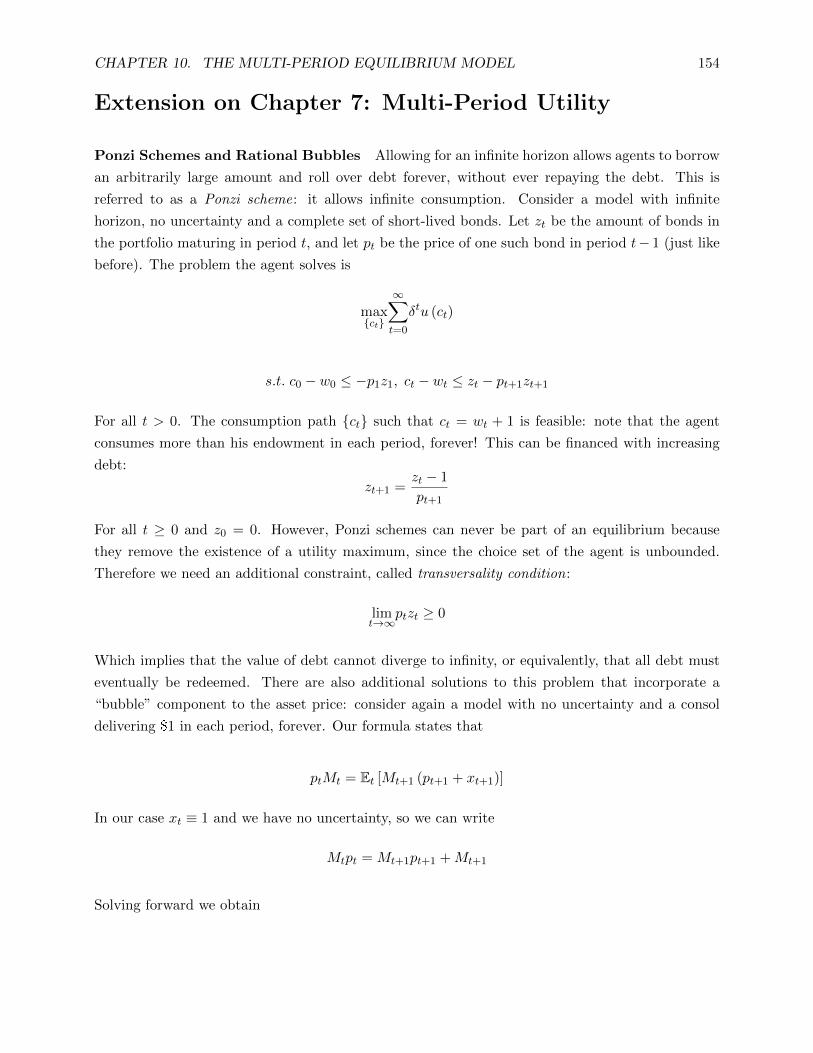
CHAPTER 10. THE MULTI-PERIOD EQUILIBRIUM MODEL 154
Extension on Chapter 7: Multi-Period Utility
Ponzi Schemes and Rational Bubbles Allowing for an infinite horizon allows agents to borrow
an arbitrarily large amount and roll over debt forever, without ever repaying the debt. This is
referred to as a Ponzi scheme: it allows infinite consumption. Consider a model with infinite
horizon, no uncertainty and a complete set of short-lived bonds. Let zt be the amount of bonds in
the portfolio maturing in period t, and let pt be the price of one such bond in period t− 1 (just like
before). The problem the agent solves is
maxct
∞∑t=0
δtu (ct)
s.t. c0 − w0 ≤ −p1z1, ct − wt ≤ zt − pt+1zt+1
For all t > 0. The consumption path ct such that ct = wt + 1 is feasible: note that the agent
consumes more than his endowment in each period, forever! This can be financed with increasing
debt:
zt+1 =zt − 1
pt+1
For all t ≥ 0 and z0 = 0. However, Ponzi schemes can never be part of an equilibrium because
they remove the existence of a utility maximum, since the choice set of the agent is unbounded.
Therefore we need an additional constraint, called transversality condition:
limt→∞
ptzt ≥ 0
Which implies that the value of debt cannot diverge to infinity, or equivalently, that all debt must
eventually be redeemed. There are also additional solutions to this problem that incorporate a
“bubble” component to the asset price: consider again a model with no uncertainty and a consol
delivering $1 in each period, forever. Our formula states that
ptMt = Et [Mt+1 (pt+1 + xt+1)]
In our case xt ≡ 1 and we have no uncertainty, so we can write
Mtpt = Mt+1pt+1 +Mt+1
Solving forward we obtain
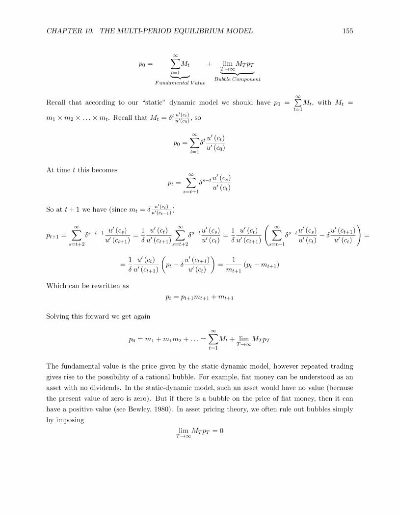
CHAPTER 10. THE MULTI-PERIOD EQUILIBRIUM MODEL 155
p0 =∞∑t=1
Mt︸ ︷︷ ︸Fundamental V alue
+ limT→∞
MT pT︸ ︷︷ ︸Bubble Component
Recall that according to our “static” dynamic model we should have p0 =∞∑t=1Mt, with Mt =
m1 ×m2 × . . .×mt. Recall that Mt = δt u′(ct)u′(c0) , so
p0 =
∞∑t=1
δtu′ (ct)
u′ (c0)
At time t this becomes
pt =
∞∑s=t+1
δs−tu′ (cs)
u′ (ct)
So at t+ 1 we have (since mt = δ u′(ct)u′(ct−1))
pt+1 =
∞∑s=t+2
δs−t−1 u′ (cs)
u′ (ct+1)=
1
δ
u′ (ct)
u′ (ct+1)
∞∑s=t+2
δs−tu′ (cs)
u′ (ct)=
1
δ
u′ (ct)
u′ (ct+1)
( ∞∑s=t+1
δs−tu′ (cs)
u′ (ct)− δu
′ (ct+1)
u′ (ct)
)=
=1
δ
u′ (ct)
u′ (ct+1)
(pt − δ
u′ (ct+1)
u′ (ct)
)=
1
mt+1(pt −mt+1)
Which can be rewritten as
pt = pt+1mt+1 +mt+1
Solving this forward we get again
p0 = m1 +m1m2 + . . . =
∞∑t=1
Mt + limT→∞
MT pT
The fundamental value is the price given by the static-dynamic model, however repeated trading
gives rise to the possibility of a rational bubble. For example, fiat money can be understood as an
asset with no dividends. In the static-dynamic model, such an asset would have no value (because
the present value of zero is zero). But if there is a bubble on the price of fiat money, then it can
have a positive value (see Bewley, 1980). In asset pricing theory, we often rule out bubbles simply
by imposing
limT→∞
MT pT = 0

CHAPTER 10. THE MULTI-PERIOD EQUILIBRIUM MODEL 156
Time Preferences We will assume a Von Neumann-Morgenstern time-separable utility function
u (c0) +∑t>0
δ(t)E [u (ct)]
Where δ (t) ∈ (0, 1] is the discount factor and δ (t) > δ (t+ 1). δ(t) also represents the intertemporal
rate of substitution. The agent solves for the whole comsumption plan (c0, c1, . . .) (for each event
on the tree) at t = 0. The two main functional forms are (1) exponential discounting: δ (t) = δt
and
E
∑t≥0
δtu (ct)
In this functional form the agent prefers early resolution of uncrtainty if this affects his actions,
and is indifferent otherwise. The other main functional form for δ (t) is the hyperbolic discounting
formulation:2
E
[u (c0) + β
∑t>0
δtu (ct)
]
Which can be expressed in recursive form and is connected to the preference for the timing of
uncertainty resolution.
We can extend our consumption-savings problem encountered in chapter 4 to a multi-period setting:
the problem becomes
maxst,atT−1
t=1
E
[T∑t=0
δtU (ct)
]s.t. cT = sT−1 (1 + rf ) + aT−1 (rT − rf )
ct + st ≤ st−1 (1 + rf ) + at−1 (rT − rf )
c0 + s0 ≤ Y0
A result similar to that found in chapter 4 holds as well:
Theorem (Merton, 1971): For CRRA utility, constant rf and i.i.d. rtTt=1 the ratioatst
is time-invariant
A “Static” Dynamic model The Debreu completeness refers to a setting in which information
is gradually revealed over many periods, but all decisions on asset trading are made at time t = 0:
decision making is static, even if the model is dynamic.
2More precisely, this is a special case of hyperbolic discounting.

CHAPTER 10. THE MULTI-PERIOD EQUILIBRIUM MODEL 157
If Arrow-Debreu securities conditional on each event A are tradable, the representative agent solves
maxct∈B(y)
∑t≥0
δtE [u (ct)]
Where B(y) is the intertemporal budget constraint (as a function of the income stream yA):
qA (yA − cA) ≤ wA
Where qA is the state price of the event A. The FOC with respect to ct(A0) = c0 yields
u′ (c0) = λ
Since π0 = 1, t (A0) = 0 and qA0 = 1. Assuming the constraint is binding, for a generic event A
instead we get
δt(A)πAu′ (cA) = λqA
Therefore we obtain the equilibrium stochastic discount factor:
qAπA
= δt(A)u′ (cA)
u′ (c0)≡Mt(A) (A)
We call the vector Mt the multi-period stochastic discount factor. Note that this can be written as
Mt(A) (A) = δt(A)u′ (cA)
u′ (c0)=
(δu′(cψ1(A)
)u′ (c0)
)︸ ︷︷ ︸
mψ1(A)
·
(δu′(cψ2(A)
)u′(cψ1(A)
))︸ ︷︷ ︸mψ2(A)
· · ·
δ u′(cψt(A)(A)
)u′(cψt(A)−1(A)
)
︸ ︷︷ ︸mψt(A)(A)
=
t(A)∏t=1
mψt(A)

CHAPTER 10. THE MULTI-PERIOD EQUILIBRIUM MODEL 158
Where mψt(A) is the usual “one-period ahead” stochastic discount factor. The fundamental pricing
formula for an asset x paying a cash flow streamxjt
∞t=1
is just
pj =∞∑t=1
E[Mtx
jt
]
If the representative agent is risk-neutral, Mt = δt and
pj =∞∑t=1
δtE[xjt
]

Bibliography
[1] Markus K. Brunnermeier, Lecture Notes for the course FIN 501: Asset Pricing, 2013.
[2] Jakub Jurek, Lecture Notes for the course FIN 521: Fixed Income Models and Appli-
cations, 2012.
[3] John H. Cochrane, Asset Pricing revised edition, Princeton University Press, 2002.
[4] John Y. Campbell, Andrew W. Lo, A. Craig McKinay, The Econometrics of Financial
Markets, Princeton University Press, 1996.
[5] Robert L. McDonald, Derivatives Markets, Pearson series in finance, 2009.
[6] Kerry E. Back, Asset Pricing and Portfolio Choice Theory, Oxford University Press,
2010.
[7] Testing Merton’s Model for Credit Spreads on Zero-Coupon Bonds, Gordon Gemill,
2003.
[8] Stephen Morris, Lecture Notes for the course ECO 317: The Economics of Uncertainty,
2011.
[9] Edwin J. Elton, Martin J. Gruber, Deepak Agrawal, and Christopher Mann, Explain-
ing the Rate Spread on Corporate Bonds, Journal of Finance, 2001.
[10] John Y. Campbell and Robert J. Shiller, Valuation Ratios and the Long-Run Stock
Market Outlook, The Journal of Portfolio Management, 1998.
159