asset liquidity and stock liquidityapps.olin.wustl.edu/faculty/gopalan/asset_stock_liquidity.pdf ·...
TRANSCRIPT

JOURNAL OF FINANCIAL AND QUANTITATIVE ANALYSIS Vol. 47, No. 2, Apr. 2012, pp. 333–364COPYRIGHT 2012, MICHAEL G. FOSTER SCHOOL OF BUSINESS, UNIVERSITY OF WASHINGTON, SEATTLE, WA 98195doi:10.1017/S0022109012000130
Asset Liquidity and Stock Liquidity
Radhakrishnan Gopalan, Ohad Kadan, and Mikhail Pevzner∗
Abstract
We study the relation between asset liquidity and stock liquidity. Our model shows that therelation may be either positive or negative depending on parameter values. Asset liquidityimproves stock liquidity more for firms that are less likely to reinvest their liquid assets(i.e., firms with less growth opportunities and financially constrained firms). Empirically,we find a positive and economically large relation between asset liquidity and stock liquid-ity. Consistent with our model, the relation is more positive for firms that are less likely toreinvest their liquid assets. Our results also shed light on the value of holding liquid assets.
I. Introduction
An asset is liquid if it can be converted into cash quickly and at a low cost.1
This definition applies both to real assets and to financial assets. Recent years haveseen a secular increase in both stock liquidity and asset liquidity as measured bythe level of cash on the firm’s balance sheet (Chordia, Roll, and Subrahmanyam(2007), Foley, Hartzell, Titman, and Twite (2007)). Furthermore, during the re-cent financial crisis, there was a decline in the liquidity of the assets of financialfirms (e.g., mortgage backed securities) and in the liquidity of their stock.2 An in-teresting question that arises is whether these 2 trends are related. More generally,
∗Gopalan, [email protected], Kadan, [email protected], Olin Business School, Washington Uni-versity in St. Louis, Campus Box 1133, St. Louis, MO 63130; and Pevzner, [email protected],School of Management, George Mason University, 4400 University Dr., MS 5F4, Fairfax, VA 22030.We thank Joel Hasbrouck for graciously providing data on stock liquidity measures and VanderbiltUniversity’s Financial Markets Research Center for making available the data on bid-ask spreads.We are also grateful to Viral Acharya, Hendrik Bessembinder (the editor), Tarun Chordia, PaoloFulghieri, Adriano Rampini, Gideon Saar (the referee), Ronnie Sadka, Mark Seasholes, and Avi Wohl;to seminar participants at American University, Barclays Global Investors, the 2009 European FinanceAssociation meetings at Bergen and our discussant Erik Theissen, the 2009 Financial IntermediationResearch Society conference at Prague and our discussant Sugato Bhattacharya, Hong Kong Univer-sity of Science and Technology, George Mason University, Nanyang Technological University, Singa-pore Management University, the 2009 Microstructure conference at the Swiss National Bank and ourdiscussant Gunther Wuyts, and Washington University for very helpful comments; and to Engin Koseand Anirudh Jonnavitula for assistance with data collection.
1This definition dates back to Keynes ((1930), p. 67) who considered one asset as more liquid thananother “if it is more certainly realizable at short notice without loss.”
2See Boehmer, Jones, and Zhang (2009) for some evidence of lower stock liquidity for financialfirms during the crisis period even after short sale constraints were removed.
333

334 Journal of Financial and Quantitative Analysis
is there a relation between the liquidity of the firm’s assets and the liquidity offinancial claims on the assets? By addressing this question we highlight howcorporate finance decisions can affect stock liquidity.
We argue that the balance sheet equivalence between the value of assets andliabilities/equity may not carry over to their respective liquidities. We formalizethis point in a model that shows how managerial investment decisions can affectstock liquidity by converting liquid assets into illiquid ones. In our model, a firmhas assets composed of cash, an illiquid project, and a growth option. The man-ager decides on the optimal allocation of cash between investment in the growthoption and payment of dividends. A more productive growth option implies moreinvestment, but firm financial constraints may limit the amount of investment.Reflecting frictions associated with raising external capital, we assume that thereturns to investment are higher when financed with internal cash. The liquid-ity of the firm’s stock is determined in a market similar to that in Kyle (1985).Managerial investment decisions affect the uncertainty of future cash flows, andconsequently stock liquidity as measured by Kyle’s lambda (the sensitivity ofprices to order flow).
Our 1st result shows that the relation between asset liquidity (the proportionof cash on the firm’s balance sheet) and stock liquidity can be either positive ornegative depending on parameter values. On the one hand, more cash lowers val-uation uncertainty associated with assets-in-place, and it improves stock liquidity.On the other hand, more cash also implies more future investments, since returnsto investment of internal cash are higher. This leads to greater uncertainty aboutfuture assets and hence lower stock liquidity. Thus, our model highlights how therelation between asset liquidity and stock liquidity depends on the tendency ofthe firm to invest. The relation is more positive (or less negative) for firms that areless likely to convert liquid assets into uncertain investments: firms with fewergrowth opportunities and those that are financially constrained.
We next turn to empirically testing the model’s predictions. While our theo-retical measure of stock liquidity is Kyle’s (1985) lambda, there is no unanimityin the literature on how to empirically measure stock liquidity. In our tests we em-ploy 4 alternative measures of stock liquidity: the illiquidity measure proposed byAmihud (2002), the implicit bid-ask spread proposed by Roll (1984) as estimatedby Hasbrouck (2009), the effective bid-ask spread calculated from intraday data,and the Pastor-Stambaugh (2003) measure.3 While stock liquidity is determinedon a daily basis, measures of asset liquidity are only recorded periodically. Hence,in our tests we use annual averages of the 4 stock liquidity measures.
To measure asset liquidity, we sort the firm’s assets based on their liquidityand assign liquidity scores of between 0 and 1 to each asset class. We then calcu-late a weighted liquidity score for the firm using the book value or market value ofthe different assets on the firm’s balance sheet as weights. Finally, we normalizethis weighted score by the lagged value of total assets of the firm. This approach
3The Pastor-Stambaugh ((2003), p. 679) measure is likely to be a noisy proxy for liquidity ofindividual stocks. We use it here to highlight the robustness of our results. We obtain similar resultswhen we use the proportion of zero-return days proposed by Lesmond, Ogden, and Trzcinka (1999)as an alternative measure of stock liquidity.
Gopalan, Kadan, and Pevzner 335
to measuring asset liquidity is similar to that of Berger and Bouwman (2009).Using this approach we come up with 4 alternative measures of asset liquiditythat vary based on the liquidity scores assigned to the different assets.
In our 1st set of tests we estimate the time-series and cross-sectional relationbetween asset liquidity and stock liquidity. These tests help us understand whichamong the 2 effects identified by our model dominates empirically. We use paneldata of all Compustat firms during the time period 1962–2005. In our main tests,we employ a model with time and firm fixed effects to understand how deviationsin asset liquidity and stock liquidity for individual firms from their sample averagevalues are related. Our results indicate that after controlling for known determi-nants of stock liquidity, there is a positive, robust, and economically significantrelation between the alternative measures of asset liquidity and those of stock liq-uidity. For example, for a firm with median level of stock liquidity, a 1-standard-deviation increase in asset liquidity results in a 15.7% decrease in Amihud’s(2002) illiquidity measure. This relation is present in different industries and indifferent time periods. Using the Fama-MacBeth (1973) approach, we also finda strong, positive relation between asset liquidity and stock liquidity in the crosssection. Thus, our empirical analysis shows that, on average, the balance sheetrelation between asset liquidity and stock liquidity does hold. Improvements inasset liquidity decrease the uncertainty related to assets-in-place more than theyincrease the uncertainty about future investments. Moreover, asset liquidity ap-pears to be a strong empirical determinant of stock liquidity.
The 2nd prediction of our model is that the relation between asset liquidityand stock liquidity should be less positive for firms with more growth oppor-tunities. Using market-to-book (MB) ratio and capital expenditure (CAPEX) toidentify growth firms, we find that the relation between asset liquidity and stockliquidity is indeed less positive for firms with more growth opportunities.
To further explore how the relation between asset liquidity and stock liquid-ity relates to investment decisions, we carry out an event study around seasonedequity offerings (SEOs). Eckbo, Masulis, and Norli (2000) document an increasein stock liquidity following an SEO. An SEO leads to an immediate inflow ofcash and an increase in asset liquidity. Our model predicts that the increase instock liquidity following the SEO will be lower for firms that invest the proceedsas compared to those that retain the proceeds as cash. Consistent with this predic-tion, we find that the change in stock liquidity in the post-SEO period is positivelyrelated to the fraction of the SEO proceeds the firm retains as cash at the end ofthe year.
We next test the prediction that the relation between asset liquidity and stockliquidity is more positive for financially constrained firms. Following prior litera-ture, we use firm size, the presence of credit ratings, and the probability of defaultto proxy for the presence of financial constraints. Consistent with our prediction,we find that the relation between asset and stock liquidity is more positive forsmall firms, firms without credit ratings, and firms with above-median probabilityof default. Overall our empirical analysis offers significant support for our modelpredictions.
In a frictionless Modigliani-Miller (MM) (1958) world where returns to in-vestments are independent of the source of finance, growth opportunities will not
336 Journal of Financial and Quantitative Analysis
affect the relation between asset liquidity and stock liquidity. Our evidence to thecontrary is consistent with the technology assumption in our model. Furthermore,the results provide new evidence supporting the importance of financial frictionsfor firm investment decisions. Unlike traditional tests of financial frictions, ourtests do not rely on correctly modeling firm investments.
A final implication of the relation between asset liquidity and stock liquiditythat we document is for the value of liquid assets on the firm’s balance sheet. In-deed, the effect of high cash balances in improving stock liquidity is a hithertounknown benefit of cash. If the improvements in stock liquidity that result froman increase in asset liquidity lead to higher firm value (e.g., by reducing the firm’scost of capital or by reducing the costs of providing managerial incentives), thenasset liquidity should be valuable for firms. This is especially so for firms withilliquid stock, as improvements in stock liquidity are more likely for such firms.To test this prediction we use the methodology in Faulkender and Wang (2006)and estimate the value of corporate cash holdings for firms with more and lessliquid stock. Consistent with our prediction, we find that an increase in corporatecash holdings is more valuable for firms with less liquid stock. As compared toa firm with above-median stock liquidity, a $1 increase in cash holdings is worth12c/ more for a firm with below-median stock liquidity.
The rest of the paper is organized as follows. In the next 2 sections, wedescribe our theoretical model and derive the main empirical predictions on thebasis of this model. Section IV describes our data, and our measures of stock andasset liquidity. Section V discusses empirical tests of the model, while Section VIdiscusses implications for value. Section VII concludes.
II. Model
In this section we develop a simple model that highlights the relation be-tween asset liquidity, future investments, and stock liquidity. The key feature ofthe model is that stock liquidity today depends on both the structure of the firm’sassets today and on the expectations regarding future investments.
There are 3 dates: 0, 1, and 2. At date 0, we consider a firm with assets-in-place whose value is normalized to $1. The assets comprise cash of value $α anda project of value $[1 − α], (α ∈ [0, 1]). We refer to α as the “asset liquidity”of the firm. Each dollar of the project will return x units of cash at date 2, wherex= μx + εx, and εx ∼ N
(0, σ2
x
).
At date 1, the manager decides on the allocation of the cash between aninterim dividend and a new project. We assume that the manager’s objective isaligned with that of the current shareholders of the firm. Let γ ≥ 0 represent thefraction of the cash invested in the new project, and 1−γ the fraction of cash thatis paid out as dividends. Note that γ > 1 indicates investment in excess of thecash available with the firm at date 0. This will happen if the firm raises outsidefinance to invest in the project (similar to Miller and Rock (1985)).
The output from investing a dollar amount αγ in the project is given by thestochastic production function
y = kαh (γ) (1 + εy) ,(1)
Gopalan, Kadan, and Pevzner 337
where εy ∼ N(0, σ2y ) is an unexpected shock to production. Thus, the expected
output from the project is kαh (γ). We assume that h (·) > 0, h′ (·) > 0, andh′′ (·) < 0.
Note that the expected output is concave in the fraction of cash invested inthe project, γ. In other words, the marginal returns to investment depend on thesource of finance. Marginal returns are higher if the firm has a high cash balanceand uses part of it to invest in the project (instances when γ is low) as compared towhen the firm raises external finance to invest in the project (instances when γ ishigh). This is a departure from an MM (1958) world, and we use this assumptionto capture the presence of costs of raising external finance in a reduced form.These costs reduce the marginal returns from investing outside cash.
We also assume that h′ (0) = ∞, implying that some positive investmentis optimal. Parameter k > 0 measures productivity. A higher k indicates highermarginal productivity at all investment levels, and thereby captures better growthopportunities. We let the correlation between εx and εy be ρ ≥ 0.4 At date 2 aliquidating dividend is paid to the equity holders. All agents are risk neutral, andthe risk-free interest rate is 0.
At date 0, the firm’s stock is traded in a market a la Kyle (1985). Specifi-cally, there are 3 types of traders: an insider, noise traders, and a market maker.We assume that the insider knows the actual realizations of both εx and εy.5 Noisetraders are uninformed and trade an exogenous amount distributed according tou ∼ N
(0, σ2
u
), where u is uncorrelated with either x or y. The market maker
observes the total order flow (both informed and uninformed) but cannot distin-guish between the two. As in Kyle, we assume that the market maker sets a priceequal to the expectation of firm value conditional on the observed order flow. Theinsider trades to maximize his profit, using the noise traders to hide his trades.
We solve the model backwards, restricting attention to equilibria, in whichboth the market maker and the insider use linear strategies. At date 1 the manageroptimally decides on the allocation of cash between interim dividend and invest-ment. Expected firm value as a function of the fraction of cash invested in the newproject, γ, is
V (γ) ≡ (1− α)μx + kαh (γ) + α (1− γ) .(2)
The 1st term represents the expected cash flow from the existing project. The 2ndand 3rd terms represent the expected cash flows from the new project and theinterim dividend, respectively. Thus, the manager’s problem is
maxγ≥0
V (γ) .
The 1st-order condition implies that the optimal proportion of cash invested is
γ∗ = h′−1
(1k
).(3)
4We limit ρ to nonnegative values, as we believe that better represents reality. Our results continueto hold for negative values of ρ as long as it is larger than some lower bound.
5Our results are robust to assuming that the insider obtains a partially informative signal aboutεx and εy. We assume perfect knowledge to limit the complexity of the analysis.
338 Journal of Financial and Quantitative Analysis
The 2nd-order condition is satisfied due to the concavity of h(·). Firms with betterinvestment opportunities invest a higher proportion of their cash:
∂γ∗
∂k= − 1
k2h′′(
h′−1
(1k
)) > 0.(4)
Consider now the trading in the firm’s shares at date 0. Both the marketmaker and the insider anticipate the optimal investment/payout decision of themanager at date 1. As a result, the expected firm value is V(γ∗). The variance ofthe firm value at time 0 is given by
σ20 ≡ (1− α)2 σ2
x + α2k2h (γ∗)2 σ2y + 2α (1− α) kh (γ∗)σxσyρ.(5)
The 1st term reflects the variability of the value of the assets-in-place. The 2ndterm reflects the variability of the expected investment, taking into account theoptimization of the manager. Finally, the 3rd term reflects the contribution of thecorrelation between the value of the current and future projects. In equilibrium,the market maker uses a linear pricing function with slope equal to Kyle’s (1985)lambda (λ). That is, lambda measures the price impact per $1 of order flow and isa conventional measure of stock illiquidity. Applying the results in Kyle, we have
λ =12σ0
σu,(6)
where, unlike in Kyle’s original model, σ0 is endogenous and given by equa-tion (5). As usual, λ is large when σ0 is large in comparison to σu (i.e., whenvariations in fundamentals are large relative to variations in noise trading).
Our 1st result illustrates how asset liquidity is related to stock liquidity inour model.
Proposition 1. The relation between asset liquidity and stock liquidity can beeither positive or negative. Higher asset liquidity is associated with higher stockliquidity (lower λ) if and only if α < α, where
α ≡ σ2x − kh (γ∗)σxσyρ
σ2x + k2h (γ∗)2 σ2
y − 2kh (γ∗)σxσyρ,
and γ∗ is given by equation (3).
All proofs are presented in Appendix A. An increase in α has 2 conflictingeffects on the variance of the firm’s cash flow, σ0. First, a higher α correspondsto a higher proportion of cash within assets-in-place, contributing to a reductionin σ0. However, a higher α also implies that the manager has more internal cashto invest in the project. Since returns to investment are higher for internal cash,this implies more investment. This contributes to an increase in σ0. As long as αis small enough (smaller than α), the 1st effect dominates, and an increase in αtranslates into higher stock liquidity. Once α becomes sufficiently large, the 2ndeffect dominates and an increase in α lowers stock liquidity.
Gopalan, Kadan, and Pevzner 339
We next study how the relation between asset liquidity and stock liquidityvaries in the cross section. Our focus is on studying how variations in growthopportunities, financial constraints, and correlation in asset returns affect thisrelation. For this analysis we first restrict attention to the case where α ≤ 0.5.6
The results when α > 0.5 are identical under some additional parameter restric-tions. We discuss this further at the end of the section.
Recall that a higher k indicates higher marginal productivity at all investmentlevels, and hence better growth opportunities.
Proposition 2. The relation between asset liquidity and stock liquidity is lesspositive (or more negative) for firms with more growth opportunities (higher k).
To understand the intuition for this result it is useful to consider the firm asa portfolio of assets-in-place and a new project. An increase in growth opportu-nities (higher k) affects the volatility of this portfolio (σ0) in 3 ways. First, for agiven α, a firm with higher k obtains a higher expected output for every dollarinvested in the new project. Second, from expression (4), higher k implies that alarger fraction of the cash balance is invested in the project (higher γ∗). Third,the increase in the investment in the new project from a higher k increases thecontribution of the correlation term to the volatility of the portfolio.7 Thus, these3 effects reinforce each other, leading to an increase in σ0 relative to σu, therebyreducing stock liquidity.
Note that this result depends critically on our assumption that returns to in-vestment are concave in γ. In the neoclassical world of MM (1958), the produc-tion function is concave in αγ rather than in γ. In such a scenario, the optimal levelof investment, and thereby the uncertainty associated with future investment, isunaffected by the amount of cash held by the firm. Thus, growth opportunities donot affect the relation between asset liquidity and stock liquidity. Empirical testsof Proposition 2 can hence serve as validation of our technology assumption.
We next consider the effect of financial constraints on the relation betweenasset liquidity and stock liquidity. Our assumption of differential returns to invest-ment of internal versus external cash can be considered as representing costs ofraising external finance. Still, to better highlight the comparative statics of thepresence of financial constraints, we model such constraints by assuming thatthere exists a γ > 0 such that γ ≤ γ. This can be interpreted as representinga precautionary savings motive for financially constrained firms or a hard con-straint on the amount of external finance that a firm can raise. Note that a firm thatfaces binding financial constraints will have γ∗= γ. Thus, in general, the optimalinvestment level is given by
γ∗ = min
(γ, h′−1
(1k
)).(7)
6This corresponds to assuming that the majority of the firm’s assets are not perfectly liquid. Suchan assumption is consistent with our data, where cash and marketable securities on average constitute14.2% of book value of total assets.
7An increase in project size will lead to an increase in the correlation term only if α < 0.5. As wediscuss later, when α > 0.5, this effect is reversed.

340 Journal of Financial and Quantitative Analysis
The following proposition derives the effect of financial constraints on therelation between asset liquidity and stock liquidity.
Proposition 3. The relation between asset liquidity and stock liquidity is morepositive (or less negative) for financially constrained firms.
Intuitively, a binding upper bound on γ∗ means that for a constrained firm, alower proportion of each additional dollar of cash is invested in a new project, re-ducing the total volatility of the firm, σ0. Thus, the relation between asset liquidityand stock liquidity is more positive.
We now discuss the robustness of our results when α > 0.5 (i.e., when cashand other liquid assets dominate the balance sheet of the firm). In this case we findthat Propositions 2 and 3 still apply subject to an additional parameter restriction,which, among other things, depends on the structure of the production function.8
The intuition for the additional restriction is as follows: When α > 0.5, the newproject is likely to be “big” relative to assets-in-place. In such a situation, an in-crease in the size of the new project resulting from an increase in k will lead to areduction in the contribution of the covariance term to the volatility of the firm’scash flow. This happens because the covariance term is maximized at α = 0.5.The other 2 effects discussed under Proposition 2 are unaffected. The parameterrestriction ensures that the covariance effect does not dominate the other 2 effects.
Finally, the following proposition discusses how the relation between assetliquidity and stock liquidity depends on ρ, the extent of correlation between thecash flows from assets-in-place and new projects.
Proposition 4. If α < 0.5 (α > 0.5), the relation between asset liquidity andstock liquidity is more (less) positive for firms with a low (high) ρ.
When α < 0.5, the covariance between the assets-in-place and the newproject makes the relation between asset liquidity and stock liquidity less positive.Since the covariance term is increasing in ρ, it follows that the relation betweenasset liquidity and stock liquidity is more positive for firms with a low ρ. A similarlogic applies in the case when α > 0.5.
III. Empirical Implications
In this section, we describe the main empirical implications of our model.From Proposition 1 we know that the relation between asset liquidity and stockliquidity can be either positive or negative. While a higher proportion of liquidassets on the balance sheet reduces the uncertainty regarding assets-in-place, italso facilitates more future investment, thereby increasing the level of uncertainty.
8For example, it can easily be verified using equation (A-3) in Appendix A that Proposition 2continues to hold when α > 0.5 as long as
ρ ≤4αkh (γ∗)2 σ2
y + 4αk2h (γ) h′ (γ∗)dγ∗
dk
2 (2α− 1)σxσy
(h (γ∗) + kh′ (γ∗)
dγ∗
dk
) .
Gopalan, Kadan, and Pevzner 341
These 2 effects influence stock liquidity in opposite directions. In our empiricalanalysis we test to see which effect dominates.
Proposition 2 implies that the relation between asset liquidity and stock liq-uidity is less positive for firms with more growth opportunities. We use firmCAPEX and MB ratios to proxy for the level of growth opportunities. Our 1stprediction follows.
Prediction 1. The relation between asset liquidity and stock liquidity is lesspositive for firms with high CAPEX and high MB ratios.
As a further test of how managerial investment decisions affect the relationbetween asset liquidity and stock liquidity, we study the changes in stock liquidityfollowing instances of firm financing. Say, when a firm raises finance through anSEO, the cash infusion is likely to result in high cash balances relative to totalassets and hence high asset liquidity. However, if the manager is expected to investthe cash in projects and growth opportunities, then despite the high asset liquidity,there is likely to be a lot of uncertainty regarding future value. The rationale of ourmodel suggests that the improvement in stock liquidity following firm financingdepends on the future utilization of the proceeds.
Prediction 2. The improvement in stock liquidity following financing dependson the extent to which the proceeds are retained as cash.
Proposition 3 shows that the relation between asset liquidity and stock liq-uidity is more positive for firms that face constraints in raising external finance.We use firm size and the presence of credit ratings to identify constrained firms.Smaller firms and firms without credit ratings are more likely to face constraintsin raising external finance. Furthermore, firms that are closer to financial distressare not only likely to face constraints in raising external finance, but they are alsolikely to be subject to an underinvestment problem (Myers (1977)).9 For suchfirms as well, we expect the relation between asset liquidity and stock liquidityto be more positive. We proxy for firm financial distress using a modified versionof the Merton-KMV expected default probability as first proposed in Bharath andShumway (2008). Thus our 3rd prediction follows.
Prediction 3. The relation between asset liquidity and stock liquidity will bemore positive for financially constrained firms, in particular for smaller firms,firms without credit ratings, and firms with higher default likelihood.
IV. Data and Liquidity Measures
To test our predictions we construct a sample that spans 1962–2005. Ouranalysis focuses on annual firm-level data for all Compustat firms. We obtain datafor 3 measures of stock liquidity from Joel Hasbrouck’s Web site (http://people.stern.nyu.edu/jhasbrou/). We use TAQ data to construct one of our stock liquidity
9An alternative view emphasizes agency conflicts when firms are in financial distress and arguesthat asset liquidity may give managers of such firms greater discretion. Managers may be able tosustain inefficient operations by liquidating the assets (see DeAngelo, DeAngelo, and Wruck (2002)).Our empirical tests will help distinguish this view from the one described in the text.

342 Journal of Financial and Quantitative Analysis
measures. We complement these data with daily stock returns and trading volumefrom the Center for Research in Security Prices (CRSP) and annual firm finan-cial data from Compustat. Finally, we use the Securities Data Company (SDC)database to identify SEOs. Apart from availability of liquidity measures and fi-nancial information in Compustat, we also limit our sample to firms with bookvalue of assets greater than $5 million and with a minimum of 2 years of finan-cial data. These restrictions ensure that very small firms do not disproportionatelyinfluence our results.
We use 4 popular measures of stock liquidity. The first is the illiquiditymeasure proposed by Amihud (2002). Since the raw Amihud measure is highlyskewed, we use the square root version of the raw measure in our empiricalanalysis. For every stock in our sample and for every year it is calculated as
ILLIQi,t =1
Ni,t
Ni,t∑j=1
√|Ri, j|
VOLi, j Pi, j−1,
where Ni,t is the number of trading days for stock i during year t, Ri, j is the returnon day j, VOLi, j is trading volume in millions of shares, and Pi, j−1 is the closingstock price. ILLIQ is a price impact measure. It captures the stock return per $1million of trading volume. This measure is constructed along the lines of Kyle’s(1985) “lambda,” with the important difference of using volume instead of signedorder flow. We obtain the annual average ILLIQ measure for all the stocks in oursample from Joel Hasbrouck’s Web site (http://people.stern.nyu.edu/jhasbrou/).
Our 2nd measure of stock liquidity is the implicit bid-ask spread, s, firstproposed in Roll (1984). This measure is calculated as the square root of thenegative daily autocorrelation of individual stock returns, that is,
si,t =√−cov(Ri, j,Ri, j−1).
Roll shows that this measure proxies for 1/2 of the bid-ask spread assuming thatthe fundamental value of the security is fixed through time and order flow is iden-tically and independently distributed. Since the autocorrelation of stock returnsis often positive, this measure is not well defined in many cases. To overcomethis problem, Hasbrouck (2009) introduces a Gibbs sampler estimate of Roll’smeasure. Hasbrouck finds that the Gibbs estimator has a correlation of 0.965 withdaily effective trading costs estimated from Trades and Quotes (TAQ) data. Weuse this Gibbs sampler estimate for our empirical analysis. We obtain data onthis measure as well from Joel Hasbrouck’s Web site (http://people.stern.nyu.edu/jhasbrou/).
Our 3rd measure of stock liquidity is the annual average effective bid-askspread, SPREAD, calculated from intraday TAQ data. The bid and ask prices areidentified from the intraday transaction data. The effective bid-ask spread for anytrade is equal to the ratio of the absolute difference between the trade price andthe midpoint of the associated quote and trade price. The effective spread is thenaveraged over the year to obtain SPREAD. This data on the average effectivespread is obtained from the Web site of the University of Vanderbilt’s FinancialMarkets Research Center (http://www.vanderbiltfmrc.org/) and is available onlyfor the subperiod 1993–2003.
Gopalan, Kadan, and Pevzner 343
Our final measure of stock liquidity is the Pastor-Stambaugh measure,PS-GAMMA. This measure was first proposed by Pastor and Stambaugh (2003).The rationale for this measure is that if a stock is illiquid, then large buy or sell vol-umes are likely to move prices. Such temporary price movements are likely to bereversed subsequently. Thus, for illiquid stocks, large buy (sell) volumes are likelyto result in subsequent negative (positive) returns. Following this logic, Pastorand Stambaugh propose regressing daily stock returns on lagged stock returnsand lagged signed volume, where the sign of lagged volume is the same as thesign of lagged stock return. The coefficient on signed volume, which on averageis expected to be negative, is a measure of stock liquidity. We obtain data on thismeasure at annual frequencies from Joel Hasbrouck’s Web site (http://people.stern.nyu.edu/jhasbrou/), where higher values of PS-GAMMA indicate a more illiquidstock. To obtain reasonable coefficients, we normalize PS-GAMMA by multiply-ing with 1,000.
Our main independent variable is a measure of asset liquidity. We assignliquidity scores of between 0 and 1 to all the assets on a firm’s balance sheet basedon their level of liquidity. We then calculate a weighted asset liquidity score usingthe book value of the different assets as weights and normalize by the laggedvalue of total assets. Using this approach we come up with 4 alternative measuresof asset liquidity. These measures differ in terms of the liquidity score assigned tothe balance sheet items.
Our 1st measure of asset liquidity assigns a liquidity score of 1 to cash andequivalents and a score of 0 to all other assets of the firm. Formally, our 1stweighted asset liquidity (WAL) measure for firm i in year t is given by
WAL1i,t =Cash & Equivalentsi,t
Total Assetsi,t−1× 1 +
Other Assetsi,t
Total Assetsi,t−1× 0.
Thus, effectively, WAL1 is the proportion of cash and equivalents to the firm’slagged total assets. Clearly, this measure leaves out a lot of information, as itpresumes that all assets other than cash and equivalents are perfectly illiquid.Nevertheless, this measure is useful because it best captures the parameter α inour model.
While cash and equivalents are perfectly liquid, noncash current assets (CA)are semiliquid. That is, they can be converted to cash relatively quickly and at alow cost. Thus, for our 2nd measure of asset liquidity, we assign a liquidity scoreof 1/2 to noncash CA. Our 2nd WAL measure is
WAL2i,t =Cash & Equivalentsi,t
Total Assetsi,t−1× 1 +
Noncash CAi,t
Total Assetsi,t−1× 0.5
+Other Assetsi,t
Total Assetsi,t−1× 0.
Noncurrent assets can be divided broadly into tangible and intangible assets. Tan-gible assets (e.g., property, plant, and equipment) are more liquid than intangibleassets (e.g., growth opportunities and goodwill). Following this logic, we calcu-late our 3rd measure by assigning a liquidity score of 1 for cash, 3/4 for noncashCA, 1/2 for tangible fixed assets, and 0 for the rest. We calculate tangible fixed
344 Journal of Financial and Quantitative Analysis
assets as the difference between the book value of total assets and the sum ofcurrent assets, and book value of goodwill and intangibles.10 This gives rise toour 3rd WAL measure,
WAL3i,t =Cash & Equivalentsi,t
Total Assetsi,t−1× 1 +
Noncash CAi,t
Total Assetsi,t−1× 0.75
+Tangible Fixed Assetsi,t
Total Assetsi,t−1× 0.5 +
Other Assetsi,t
Total Assetsi,t−1× 0.
We construct our 4th and final measure of asset liquidity to capture the liquid-ity of both assets-in-place and growth options. We construct the market-weightedasset liquidity (MWAL) measure by assigning a liquidity score of 1 to cash andequivalents, 3/4 to noncash CA, 1/2 to tangible fixed assets, and 0 to the rest. Wecalculate tangible fixed assets as the difference between the book value of totalassets and the sum of current assets and goodwill. We normalize this weightedscore by the lagged market value of total assets to obtain
MWALi,t =Cash & Equivalentsi,t
Market Assetsi,t−1× 1 +
Noncash CAi,t
Market Assetsi,t−1× 0.75
+Tangible Fixed Assetsi,t
Market Assetsi,t−1× 0.5 +
Other Assetsi,t
Market Assetsi,t−1× 0.
Note that MWAL assigns a liquidity score of 0 to growth options. Since we nor-malize the measure by the market value of assets—which is likely to includegrowth options—ceteris paribus, MWAL will be lower for firms with a higherproportion of growth options.11
We use additional independent variables to account for firm and market char-acteristics that are likely to affect stock liquidity. All variables are defined in Ap-pendix B. We control for firm size, which is an important determinant of stockliquidity, using log(MRKT CAP), for the extent of growth opportunities usingMB, and CAPEX. We also control for firm performance using return on assets,ROA, and using the annual buy-and-hold abnormal return during the previousyear, BHAR. Firms with more transparent earnings and firms with better disclo-sure policies are also likely to be associated with higher stock liquidity (Diamondand Verrecchia (1991), Bhattacharya, Desai, and Venkataraman (2007)). In mostof our specifications we employ firm fixed effects, and this is likely to controlfor time-invariant differences across firms in disclosure policies. In addition, wecontrol for the quality of a firm’s earnings using the level of discretionary accrualsnormalized by lagged value of total assets, DISC ACC.12 Finally, we control forstock return volatility, log(VOLATILITY).
Table 1 presents summary statistics for the key variables in our sample. Toreduce the effects of outliers, all of our variables are winsorized at the 1% level.
10We obtain book values of goodwill and intangibles from Data204 and Data33 in Compustat.11We calculate the market value of assets as the sum of the book value of assets and the market
value of equity less the book value of equity.12The reported results use the signed discretionary accruals. The results are similar when using the
absolute value of the discretionary accruals instead (not reported, but are available from the authors).
Gopalan, Kadan, and Pevzner 345
TABLE 1
Summary Statistics
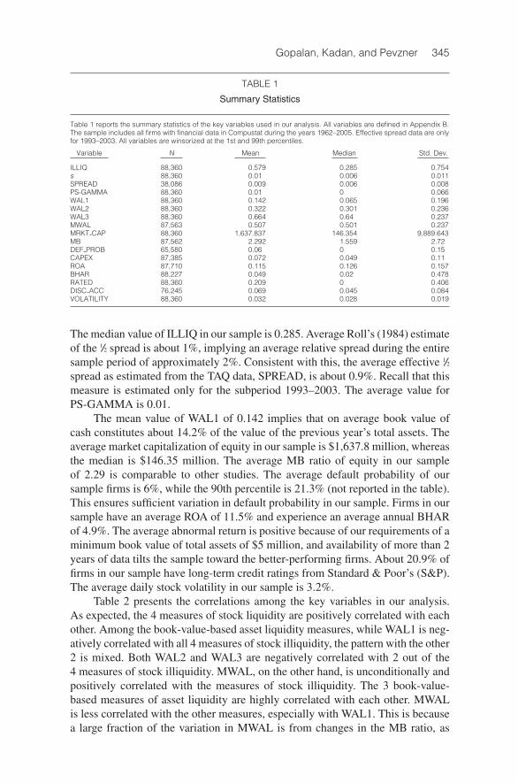
Table 1 reports the summary statistics of the key variables used in our analysis. All variables are defined in Appendix B.The sample includes all firms with financial data in Compustat during the years 1962–2005. Effective spread data are onlyfor 1993–2003. All variables are winsorized at the 1st and 99th percentiles.
Variable N Mean Median Std. Dev.
ILLIQ 88,360 0.579 0.285 0.754s 88,360 0.01 0.006 0.011SPREAD 38,086 0.009 0.006 0.008PS-GAMMA 88,360 0.01 0 0.066WAL1 88,360 0.142 0.065 0.196WAL2 88,360 0.322 0.301 0.236WAL3 88,360 0.664 0.64 0.237MWAL 87,563 0.507 0.501 0.237MRKT CAP 88,360 1,637.837 146.354 9,889.643MB 87,562 2.292 1.559 2.72DEF PROB 65,580 0.06 0 0.15CAPEX 87,385 0.072 0.049 0.11ROA 87,710 0.115 0.126 0.157BHAR 88,227 0.049 0.02 0.478RATED 88,360 0.209 0 0.406DISC ACC 76,245 0.069 0.045 0.084VOLATILITY 88,360 0.032 0.028 0.019
The median value of ILLIQ in our sample is 0.285. Average Roll’s (1984) estimateof the 1/2 spread is about 1%, implying an average relative spread during the entiresample period of approximately 2%. Consistent with this, the average effective 1/2spread as estimated from the TAQ data, SPREAD, is about 0.9%. Recall that thismeasure is estimated only for the subperiod 1993–2003. The average value forPS-GAMMA is 0.01.
The mean value of WAL1 of 0.142 implies that on average book value ofcash constitutes about 14.2% of the value of the previous year’s total assets. Theaverage market capitalization of equity in our sample is $1,637.8 million, whereasthe median is $146.35 million. The average MB ratio of equity in our sampleof 2.29 is comparable to other studies. The average default probability of oursample firms is 6%, while the 90th percentile is 21.3% (not reported in the table).This ensures sufficient variation in default probability in our sample. Firms in oursample have an average ROA of 11.5% and experience an average annual BHARof 4.9%. The average abnormal return is positive because of our requirements of aminimum book value of total assets of $5 million, and availability of more than 2years of data tilts the sample toward the better-performing firms. About 20.9% offirms in our sample have long-term credit ratings from Standard & Poor’s (S&P).The average daily stock volatility in our sample is 3.2%.
Table 2 presents the correlations among the key variables in our analysis.As expected, the 4 measures of stock liquidity are positively correlated with eachother. Among the book-value-based asset liquidity measures, while WAL1 is neg-atively correlated with all 4 measures of stock illiquidity, the pattern with the other2 is mixed. Both WAL2 and WAL3 are negatively correlated with 2 out of the4 measures of stock illiquidity. MWAL, on the other hand, is unconditionally andpositively correlated with the measures of stock illiquidity. The 3 book-value-based measures of asset liquidity are highly correlated with each other. MWALis less correlated with the other measures, especially with WAL1. This is becausea large fraction of the variation in MWAL is from changes in the MB ratio, as

346 Journal of Financial and Quantitative Analysis
TABLE 2
Correlations
Table 2 reports the correlations between the key variables used in our analysis. All variables are defined in Appendix B.The sample includes all firms with financial data in Compustat during the years 1962–2005. Effective spread data are onlyfor 1993–2003. All variables are winsorized at the 1st and 99th percentiles.
ILLIQ s SPREAD PS-GAMMA WAL1 WAL2 WAL3 MWAL log(MRKT CAP)t−1
ILLIQ 1.000s 0.811 1.000SPREAD 0.830 0.884 1.000PS-GAMMA 0.384 0.330 0.314 1.000WAL1 −0.086 −0.007 −0.021 −0.028 1.000WAL2 −0.020 0.051 0.066 −0.009 0.839 1.000WAL3 −0.030 0.028 0.051 −0.009 0.636 0.791 1.000MWAL 0.280 0.194 0.266 0.077 0.041 0.201 0.414 1.000log(MRKT CAP)t−1 −0.130 −0.134 −0.173 −0.032 −0.026 −0.057 −0.028 −0.135 1.000MBt−1 −0.158 −0.078 −0.122 −0.034 0.278 0.253 0.212 −0.408 0.161DEF PROB 0.288 0.299 0.257 0.132 −0.100 −0.119 −0.167 0.025 −0.065CAPEX −0.048 −0.024 −0.017 −0.015 0.041 0.006 0.225 0.061 0.002RATED −0.331 −0.329 −0.413 −0.091 −0.205 −0.302 −0.207 −0.126 0.245ROA −0.139 −0.209 −0.184 −0.041 −0.297 −0.148 −0.015 0.034 0.105BHARt−1 −0.119 −0.147 −0.139 −0.050 0.185 0.215 0.206 −0.098 0.012log(VOLATILITY)t−1 0.375 0.507 0.497 0.148 0.314 0.335 0.164 0.046 −0.155DISC ACC 0.070 0.118 0.124 0.035 0.143 0.312 0.296 0.078 −0.055
MBt−1 DEF PROB CAPEX RATED ROA BHARt−1 log(VOLATILITYt−1)
MBt−1 1.000DEF PROB −0.079 1.000CAPEX 0.075 −0.061 1.000RATED −0.004 0.003 0.003 1.000ROA −0.079 −0.175 0.101 0.144 1.000BHARt−1 0.196 −0.231 0.081 −0.032 0.079 1.000log(VOLATILITY)t−1 0.089 0.331 −0.007 −0.364 −0.345 0.128 1.000DISC ACC 0.110 0.057 0.105 −0.158 −0.093 0.083 0.225
can be seen from the correlation between MWAL and MB of −0.408.13 Manyof our control variables are also significantly correlated with the stock illiquiditymeasures, justifying the need to include them in the regressions.
V. Empirical Results
A. The Basic Effect
We begin our empirical analysis by testing whether on average there is apositive or negative relation between asset liquidity and stock liquidity. To do thiswe estimate panel models with both firm fixed effects and time effects as follows:
Yi,t = α + βXi,t + γCONTROLSi,t + μi + μt + εi,t.(8)
Here Yi,t is 1 of the 4 measures of stock liquidity for firm i during year t, Xi,t is1 of the 4 asset liquidity measures, μi are firm fixed effects, and μt are year dummyvariables. The control variables are log(MRKT CAP), CAPEX, MB, ROA,BHAR, log(VOLATILITY), and DISC ACC. We use standard errors that are ro-bust to heteroskedasticity and clustered at the firm level.14
13Since a lot of variation in our market value measure is driven by changes in market value ofequity, we put more weight on the results with our book value measures.
14Since stock liquidity is correlated across stocks at a point in time, in alternative empirical spec-ifications we repeat our tests clustering standard errors at the year level and obtain results similar to

Gopalan, Kadan, and Pevzner 347
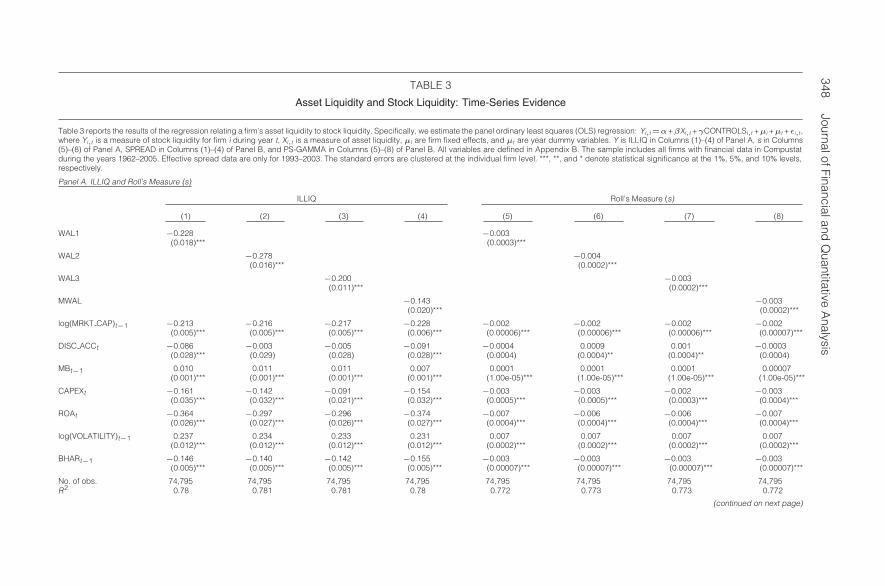
In Table 3 we estimate the average relation between asset liquidity and stockliquidity in our sample. We employ the 16 different combinations of asset liquidityand stock liquidity measures. Since all 4 measures of stock liquidity are in factmeasures of stock illiquidity, the sign of the relation between asset and stockliquidity is opposite to the sign of the coefficient.
In Panel A of Table 3 the dependent variable is either ILLIQ or s. Columns(1)–(4) have ILLIQ as the dependent variable and correspond to the 4 differentmeasures of asset liquidity: WAL1, WAL2, WAL3, and MWAL. The coefficientson all 4 measures are negative and significant. Furthermore, the results are eco-nomically significant. For example, for a firm with a median level of stock liquid-ity, a 1-standard-deviation increase in WAL1 reduces ILLIQ by 15.7%. Similarly,a 1-standard-deviation increase in MWAL reduces ILLIQ by 11.9% for a firmwith a median level of stock illiquidity. Note that the R2s in all of our regressionsare high because of the use of firm fixed effects.
All of our control variables are significant and indicate that smaller firms,firms with high MB ratio, firms with less discretionary accruals (weakly), firmsthat do not undertake large CAPEX, firms with low levels of profitability andabnormal stock returns, and those with more volatile stock have less liquid stock.
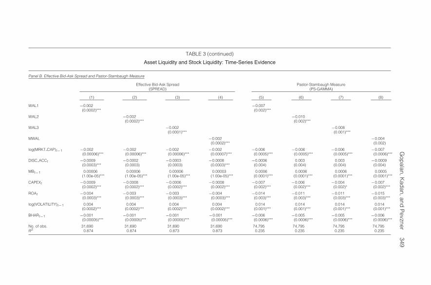
In Columns (5)–(8) of Table 3 we repeat our estimation with Roll’s (1984)measure as the dependent variable and obtain results consistent with those in theearlier columns. Here again we find that an increase in the proportion of liquidassets in the firm’s balance sheet increases stock liquidity. The results are alsoeconomically significant. For example, the estimate in Column (5) indicates thatfor a firm with the median level of stock liquidity, a 1-standard-deviation increasein WAL1 improves stock liquidity by 9.8%. In Panel B we repeat the estimationusing the SPREAD and PS-GAMMA as the dependent variables. The results aresimilar to those in the previous panel.
The results in Table 3 provide strong support for a positive average relationbetween asset liquidity and stock liquidity. This indicates that in our sample theeffect of higher asset liquidity in increasing the liquidity of assets-in-place out-weighs its effect of reducing the liquidity of future assets.15,16
To see if and how the relation between asset liquidity and stock liquiditychanges with time, in unreported tests we split our sample into 4 subperiods(1962–1975, 1976–1985, 1986–1995, and 1996–2005) and repeat our estimates.Our results indicate a positive association between asset liquidity and stock liq-uidity in all but the 1st subperiod. Furthermore, we find that the relation becomes
those reported. Alternatively, we also tried clustering standard errors both at the firm and year levels,but given the large number of fixed effects in our specifications, the estimates failed to converge.
15In unreported tests we divide our sample firms into 3 broad industry groups: Financial services(firms with Standard Industrial Classification (SIC) codes 6000–6999), Utilities (firms with SIC codes4000–4999), and Industrials (firms with SIC codes 2000–3999) and repeat our tests in the subsamples.We find that asset liquidity and stock liquidity are positively related within all 3 industry groups. Thereis some evidence that the relation is strongest among industrial firms.
16To ensure that across-industry differences in the level of cash balance do not bias our results,we repeat our tests replacing WAL1 with ABNORMAL WAL1, where ABNORMAL WAL1 is thedifference between the firm’s WAL1 and the median WAL1 of all firms in the same 3-digit SICcode industry during the year. Our results indicate a positive association between stock liquidity andABNORMAL WAL1.
348JournalofFinancialand
Quantitative
Analysis
TABLE 3
Asset Liquidity and Stock Liquidity: Time-Series Evidence
Table 3 reports the results of the regression relating a firm’s asset liquidity to stock liquidity. Specifically, we estimate the panel ordinary least squares (OLS) regression: Yi,t=α+βXi,t +γCONTROLSi,t +μi +μt +εi,t ,where Yi,t is a measure of stock liquidity for firm i during year t, Xi,t is a measure of asset liquidity, μi are firm fixed effects, and μt are year dummy variables. Y is ILLIQ in Columns (1)–(4) of Panel A, s in Columns(5)–(8) of Panel A, SPREAD in Columns (1)–(4) of Panel B, and PS-GAMMA in Columns (5)–(8) of Panel B. All variables are defined in Appendix B. The sample includes all firms with financial data in Compustatduring the years 1962–2005. Effective spread data are only for 1993–2003. The standard errors are clustered at the individual firm level. ***, **, and * denote statistical significance at the 1%, 5%, and 10% levels,respectively.
Panel A. ILLIQ and Roll’s Measure (s)
ILLIQ Roll’s Measure (s)
(1) (2) (3) (4) (5) (6) (7) (8)
WAL1 −0.228 −0.003(0.018)*** (0.0003)***
WAL2 −0.278 −0.004(0.016)*** (0.0002)***
WAL3 −0.200 −0.003(0.011)*** (0.0002)***
MWAL −0.143 −0.003(0.020)*** (0.0002)***
log(MRKT CAP)t−1 −0.213 −0.216 −0.217 −0.228 −0.002 −0.002 −0.002 −0.002(0.005)*** (0.005)*** (0.005)*** (0.006)*** (0.00006)*** (0.00006)*** (0.00006)*** (0.00007)***
DISC ACCt −0.086 −0.003 −0.005 −0.091 −0.0004 0.0009 0.001 −0.0003(0.028)*** (0.029) (0.028) (0.028)*** (0.0004) (0.0004)** (0.0004)** (0.0004)
MBt−1 0.010 0.011 0.011 0.007 0.0001 0.0001 0.0001 0.00007(0.001)*** (0.001)*** (0.001)*** (0.001)*** (1.00e-05)*** (1.00e-05)*** (1.00e-05)*** (1.00e-05)***
CAPEXt −0.161 −0.142 −0.091 −0.154 −0.003 −0.003 −0.002 −0.003(0.035)*** (0.032)*** (0.021)*** (0.032)*** (0.0005)*** (0.0005)*** (0.0003)*** (0.0004)***
ROAt −0.364 −0.297 −0.296 −0.374 −0.007 −0.006 −0.006 −0.007(0.026)*** (0.027)*** (0.026)*** (0.027)*** (0.0004)*** (0.0004)*** (0.0004)*** (0.0004)***
log(VOLATILITY)t−1 0.237 0.234 0.233 0.231 0.007 0.007 0.007 0.007(0.012)*** (0.012)*** (0.012)*** (0.012)*** (0.0002)*** (0.0002)*** (0.0002)*** (0.0002)***
BHARt−1 −0.146 −0.140 −0.142 −0.155 −0.003 −0.003 −0.003 −0.003(0.005)*** (0.005)*** (0.005)*** (0.005)*** (0.00007)*** (0.00007)*** (0.00007)*** (0.00007)***
No. of obs. 74,795 74,795 74,795 74,795 74,795 74,795 74,795 74,795R2 0.78 0.781 0.781 0.78 0.772 0.773 0.773 0.772
(continued on next page)
Gop
alan,Kad
an,andP
evzner349
TABLE 3 (continued)
Asset Liquidity and Stock Liquidity: Time-Series Evidence
Panel B. Effective Bid-Ask Spread and Pastor-Stambaugh Measure
Effective Bid-Ask Spread Pastor-Stambaugh Measure(SPREAD) (PS-GAMMA)
(1) (2) (3) (4) (5) (6) (7) (8)
WAL1 −0.002 −0.007(0.0002)*** (0.002)***
WAL2 −0.002 −0.010(0.0002)*** (0.002)***
WAL3 −0.002 −0.008(0.0001)*** (0.001)***
MWAL −0.002 −0.004(0.0002)*** (0.002)
log(MRKT CAP)t−1 −0.002 −0.002 −0.002 −0.002 −0.006 −0.006 −0.006 −0.007(0.00006)*** (0.00006)*** (0.00006)*** (0.00007)*** (0.0005)*** (0.0005)*** (0.0005)*** (0.0006)***
DISC ACCt −0.0009 −0.0002 −0.0003 −0.0008 −0.0006 0.003 0.003 −0.0009(0.0003)*** (0.0003) (0.0003) (0.0003)*** (0.004) (0.004) (0.004) (0.004)
MBt−1 0.00006 0.00006 0.00006 0.00003 0.0006 0.0006 0.0006 0.0005(1.00e-05)*** (1.00e-05)*** (1.00e-05)*** (1.00e-05)*** (0.0001)*** (0.0001)*** (0.0001)*** (0.0001)***
CAPEXt −0.0009 −0.0008 −0.0006 −0.0008 −0.007 −0.006 −0.004 −0.007(0.0002)*** (0.0002)*** (0.0002)*** (0.0002)*** (0.002)*** (0.002)*** (0.002)* (0.002)***
ROAt −0.004 −0.003 −0.003 −0.004 −0.014 −0.011 −0.011 −0.015(0.0003)*** (0.0003)*** (0.0003)*** (0.0003)*** (0.003)*** (0.003)*** (0.003)*** (0.003)***
log(VOLATILITY)t−1 0.004 0.004 0.004 0.004 0.014 0.014 0.014 0.014(0.0002)*** (0.0002)*** (0.0002)*** (0.0002)*** (0.001)*** (0.001)*** (0.001)*** (0.001)***
BHARt−1 −0.001 −0.001 −0.001 −0.001 −0.006 −0.005 −0.005 −0.006(0.00005)*** (0.00005)*** (0.00005)*** (0.00005)*** (0.0006)*** (0.0006)*** (0.0006)*** (0.0006)***
No. of obs. 31,690 31,690 31,690 31,690 74,795 74,795 74,795 74,795R2 0.874 0.874 0.873 0.873 0.235 0.235 0.235 0.235

350 Journal of Financial and Quantitative Analysis
more positive in the latter subperiods. To conserve space, we do not report theseresults, but they are available from the authors.
Since we employ firm fixed effects in all of our specifications, the correla-tions that we document are between deviations in asset liquidity and stock liquid-ity from their average value for an individual firm in our sample. Does the samerelation between asset liquidity and stock liquidity hold in the cross section aswell? To answer this question, in Table 4 we employ the Fama-MacBeth (1973)approach. We conduct annual cross-sectional regressions of stock liquidity onmeasures of asset liquidity and the full set of control variables, and report the av-erage coefficients along with the standard errors. Since stock liquidity is quite per-sistent, we adjust for autocorrelation by correcting the reported standard errors. Todo this, we follow Fama and French (2002) and Cooper, Gulen, and Schill (2008),and multiply the standard errors of the average parameters by
√(1 + ρ)/(1− ρ),
where ρ is the 1st-order autocorrelation of annual parameter estimates. To con-serve space, we suppress the coefficients on the control variables. The results inPanels A and B of Table 4 are consistent with a positive relation between asset
TABLE 4
Asset Liquidity and Stock Liquidity: Cross-Sectional Evidence
Table 4 reports the results of Fama-MacBeth (1973) regressions relating a firm’s asset liquidity to stock liquidity. Specif-ically, we estimate the annual OLS regression, Yi,t = α + βXi,t + γCONTROLSi,t + εi,t, and report the average of theannual coefficients. Here, Yi,t is a measure of stock liquidity for firm i during year t and Xi,t is a measure of asset liquidity;Y is ILLIQ in Columns (1)–(4) of Panel A, s in Columns (5)–(8) of Panel A, SPREAD in Columns (1)–(4) of Panel B, andPS-GAMMA in Columns (5)–(8) of Panel B. The specification is similar to the ones in Panels A and B of Table 3. We sup-press the coefficients of the control variables in order to conserve space. To adjust for autocorrelation, we correct thereported standard errors of the average parameters by multiplying with
√(1 + ρ)/(1− ρ), where ρ is the 1st-order auto-
correlation in yearly parameter estimates. The sample includes all firms with financial data in Compustat during the years1962–2005. Effective spread data are only for 1993–2003. ***, **, and * denote statistical significance at the 1%, 5%, and10% levels, respectively.
Panel A. ILLIQ and Roll’s Measure (s)
ILLIQ Roll’s Measure (s)
(1) (2) (3) (4) (5) (6) (7) (8)
WAL1 –0.269 –0.004(0.089)*** (0.001)***
WAL2 –0.279 –0.005(0.129)*** (0.002)***
WAL3 –0.245 –0.004(0.049)*** (0.0009)***
MWAL –0.019 –0.002(0.035) (0.0007)***
No. of obs. 43 43 43 43 43 43 43 43
Panel B. Effective Bid-Ask Spread and Pastor-Stambaugh Measure
Effective Bid-Ask Spread Pastor-Stambaugh Measure(SPREAD) (PS-GAMMA)
(1) (2) (3) (4) (5) (6) (7) (8)
WAL1 –0.004 –0.006(0.0002)*** (0.006)
WAL2 –0.004 –0.017(0.0006)*** (0.004)***
WAL3 –0.002 –0.015(0.006)*** (0.005)***
MWAL 0.0004 –0.0001(0.003) (0.0002)
No. of obs. 12 12 12 12 43 43 43 43
Gopalan, Kadan, and Pevzner 351
liquidity and stock liquidity in the cross section. We find that 12 of the 16 coef-ficients are negative and statistically significant. The coefficient estimates are insome cases larger than the estimates in Table 3.
In summary, asset liquidity and stock liquidity are positively related bothacross time and in the cross section. This suggests that the observed WAL1 inour sample is lower than α (Proposition 1). The magnitude of the effect is alsolarge. Since asset liquidity and stock liquidity are likely to be endogenous, oneconcern with our estimates is of omitted variable bias. Say firms with growthopportunities may have high asset liquidity and stock liquidity. If we do not ad-equately control for growth opportunities, our estimates are likely to be biased.To see if our results are robust to partially controlling for endogeneity, we em-ploy the linear generalized method of moments (GMM) estimator proposed byArellano and Bond (1991). This procedure uses lagged values to instrument forasset liquidity and estimates the regression using the GMM procedure. We findthat our results are robust to using this procedure. This indicates that the positivecorrelation between asset liquidity and stock liquidity is not driven by omittedvariables bias.17
B. Growth Opportunities and the Relation between Asset Liquidityand Stock Liquidity
Having established a positive average relation between asset liquidity andstock liquidity, we now turn to test Prediction 1: The relation between asset liq-uidity and stock liquidity is less positive for firms with more growth opportunities.
In Panel A of Table 5 we use CAPEX to identify firms with growth oppor-tunities. We divide our sample into firms with above- and below-median CAPEXeach year and repeat our tests in the 2 subsamples. To conserve space, we onlyreport the results for Amihud’s (2002) stock illiquidity measure. Similar resultsobtain for the other 3 stock liquidity measures. While our specification is simi-lar to the one we employ in Table 3, we suppress the coefficients on the controlvariables other than log(MRKT CAP) to conserve space.
One way to test Prediction 1 is to repeat the estimation of equation (8) af-ter including an interaction term between the measures of asset liquidity anda dummy variable that identifies firms with high CAPEX. Prediction 1 wouldimply a positive coefficient on the interaction term. Instead of employing sucha procedure, we repeat the estimation of equation (8) on 2 subsamples of firmswith high and low CAPEX, and we test to see if the coefficient on the asset liq-uidity measure is different across the 2 subsamples. Our methodology is a moregeneral way of estimating interaction effects, because we do not constrain thecoefficients on the control variables to be the same for firms with high and lowCAPEX. Thus, our procedure is equivalent to estimating the interaction effect af-ter including a full set of interaction terms for all the control variables includingthe fixed effects.18 We employ this procedure for its generality.
17We thank Christopher Baum for suggesting this test.18To test if the relation between asset liquidity and stock liquidity is significantly different across
the 2 subsamples, we estimate a single equation with a full set of interaction terms between all
352 Journal of Financial and Quantitative Analysis
TABLE 5
Asset Liquidity and Stock Liquidity
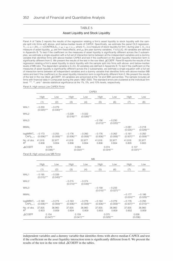
Panel A of Table 5 reports the results of the regression relating a firm’s asset liquidity to stock liquidity with the sam-ple split into firms with above- and below-median levels of CAPEX. Specifically, we estimate the panel OLS regression,Yi,t =α + βXi,t + γCONTROLSi,t +μi +μt + εi,t, where Yi,t is a measure of stock liquidity for firm i during year t, Xi,t is ameasure of asset liquidity, μi are firm fixed effects, and μt are year dummy variables. Y is ILLIQ. All variables are definedin Appendix B. To test if the coefficient on the measures of asset liquidity is significantly different across the 2 subsam-ples, we estimate a single equation with a full set of interaction terms between all the independent variables and a dummyvariable that identifies firms with above-median CAPEX and test if the coefficient on the asset liquidity interaction term issignificantly different from 0. We present the results of the test in the row titled ΔCOEFF. Panel B reports the results of theregression relating a firm’s asset liquidity to stock liquidity with the sample split into firms with above- and below-medianlevels of MB ratio. The dependent variable is ILLIQ. All variables are defined in Appendix B. To test if the coefficient on themeasures of asset liquidity is significantly different across the 2 subsamples, we estimate a single equation with a full setof interaction terms between all independent variables and a dummy variable that identifies firms with above-median MBratios and test if the coefficient on the asset liquidity interaction term is significantly different from 0. We present the resultsof the test in the row titled ΔCOEFF. All variables are winsorized at the 1st and 99th percentiles. The sample includes allfirms with financial data in Compustat during the years 1962–2005. The standard errors are clustered at the individual firmlevel. ***, **, and * denote statistical significance at the 1%, 5%, and 10% levels, respectively.
Panel A. High versus Low CAPEX Firms
CAPEX
High Low High Low High Low High Low
(1) (2) (3) (4) (5) (6) (7) (8)
WAL1 −0.200 −0.279(0.020)*** (0.030)***
WAL2 −0.228 −0.322(0.018)*** (0.026)***
WAL3 −0.156 −0.230(0.013)*** (0.020)***
MWAL −0.081 −0.218(0.025)*** (0.028)***
log(MRKT −0.173 −0.255 −0.176 −0.260 −0.176 −0.262 −0.181 −0.282CAP)t−1 (0.006)*** (0.008)*** (0.006)*** (0.008)*** (0.006)*** (0.008)*** (0.007)*** (0.009)***
No. of obs. 41,818 32,977 41,818 32,977 41,818 32,977 41,818 32,977R2 0.806 0.804 0.806 0.804 0.806 0.804 0.805 0.803
ΔCOEFF 0.079 0.094 0.074 0.137(0.036)** (0.032)*** (0.024)*** (0.037)***
Panel B. High versus Low MB Firms
MB
High Low High Low High Low High Low
(1) (2) (3) (4) (5) (6) (7) (8)
WAL1 −0.185 −0.339(0.015)*** (0.045)***
WAL2 −0.215 −0.374(0.014)*** (0.039)***
WAL3 −0.158 −0.233(0.010)*** (0.027)***
MWAL −0.177 −0.186(0.024)*** (0.028)***
log(MRKT −0.160 −0.274 −0.163 −0.279 −0.164 −0.279 −0.176 −0.293CAP)t−1 (0.006)*** (0.009)*** (0.006)*** (0.009)*** (0.006)*** (0.009)*** (0.007)*** (0.010)***
No. of obs. 37,835 36,960 37,835 36,960 37,835 36,960 37,835 36,960R2 0.803 0.809 0.804 0.809 0.803 0.809 0.802 0.809
ΔCOEFF 0.154 0.159 0.075 0.008(0.047)*** (0.041)*** (0.029)*** (0.036)
independent variables and a dummy variable that identifies firms with above-median CAPEX and testif the coefficient on the asset liquidity interaction term is significantly different from 0. We present theresults of the test in the row titledΔCOEFF in the tables.
Gopalan, Kadan, and Pevzner 353
The results in Columns (1) and (2) of Table 5 indicate that WAL1 has amore positive relation with stock liquidity for firms with below-median CAPEX(−0.279) in comparison to firms with above-median CAPEX (−0.200). The rowtitled ΔCOEFF shows that the coefficients across the 2 subsamples are signif-icantly different from each other. Qualitatively similar differences obtain fromcomparing Columns (3)–(4), (5)–(6), and (7)–(8).19
In Panel B of Table 5 we repeat the analysis using the firm’s MB ratio toproxy for the extent of growth opportunities. Since firms with a high MB ratio(above median) are likely to have more growth opportunities, following Predic-tion 1, we expect asset liquidity to have a less positive effect on stock liquidityfor such firms. Consistent with our prediction, the results in Columns (1) and (2)of Panel B show that WAL1 has a more positive relation with stock liquidity forfirms with low MB ratio. From ΔCOEFF we find that the coefficients are sig-nificantly different from each other across the 2 subsamples. In Columns (3)–(8)we repeat our estimates successively with WAL2, WAL3, and MWAL. All theresults, except for those with MWAL, show a significantly more positive effect ofasset liquidity on stock liquidity for firms with low MB ratios.
We now proceed to tests of Prediction 2. To recall, Prediction 2 suggests thatthe improvement in stock liquidity following firm financing should be greater ifthe firm retains a larger fraction of the issue proceeds as cash. To test the predic-tion, we focus on SEOs and relate the change in stock liquidity in the post-issueperiod to the fraction of issue proceeds that the firm retains as cash.
We obtain a sample of SEOs from SDC with issue date during the period1970–2006 and with nonmissing and positive values for number of primary sharesoffered, issue proceeds, and issue price. We also confine the sample to SEOswith a minimum size of $10 million. We combine the SEO data with CRSP andCompustat to obtain stock price information during the pre- and post-issue periodsand firm financial data. This procedure results in a sample of 5,756 SEOs.
The summary statistics for the key variables for this SEO sample are pro-vided in Panel A of Table 6. The average size of the issue in our sample is $103.31million, which constitutes about 31% of the book value of total assets as of the endof the previous year. We use daily stock return data to calculate ILLIQ during thepre- and post-issue periods. ILLIQ−30,0 (ILLIQ−60,0) is Amihud’s (2002) illiquid-ity measure estimated during the 30 (60) days prior to the SEO, while ILLIQ15,45
(ILLIQ15,75) represents a similar measure estimated during the 30 (60) days fol-lowing the SEO. In calculating the illiquidity measures for the post-issue period,we ignore the 15-day period immediately following the SEO to avoid any biasdue to abnormal trading immediately following the SEO. Stock liquidity signifi-cantly improves after the SEO. This is evident from the fact that ILLIQ15,45 and
19Since the normal level of CAPEX may differ across industries, we perform additional tests toensure that our results are not simply capturing across-industry differences in the relation betweenasset liquidity and stock liquidity. To do this, we repeat our tests in subsamples of firms with positiveand negative ABNORMAL CAPEX, where ABNORMAL CAPEX measures the difference betweenthe firm’s CAPEX and the median CAPEX of all firms in the same 3-digit SIC code industry duringthe year. Consistent with our reported results, we find that the relation between asset liquidity andstock liquidity is less positive in the subsample of firms with positive abnormal CAPEX. The resultsare available from the authors.
354 Journal of Financial and Quantitative Analysis
TABLE 6
Proceeds Retained in SEOs and Stock Liquidity
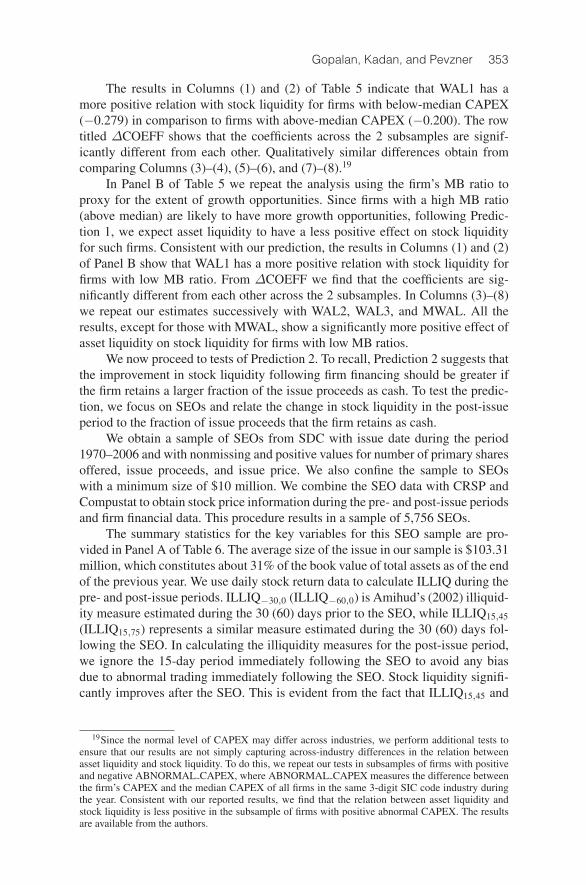
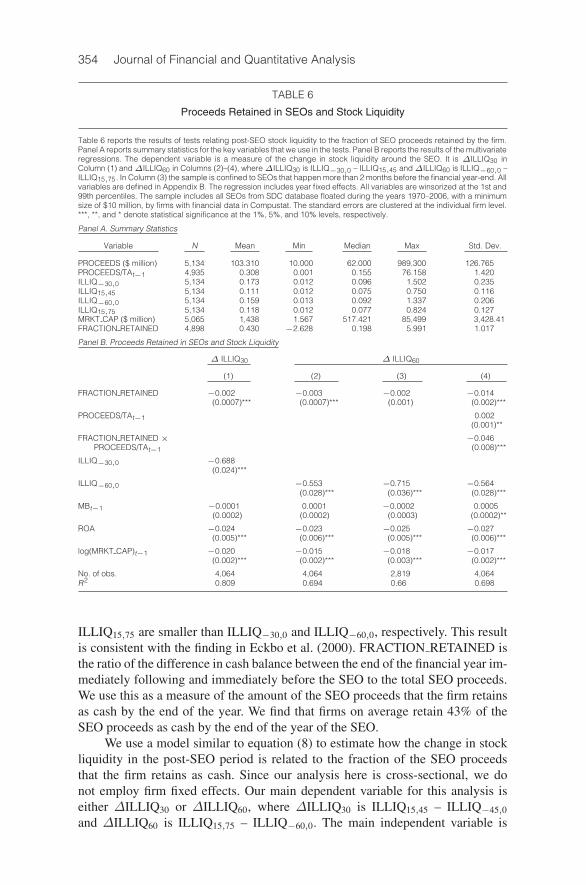
Table 6 reports the results of tests relating post-SEO stock liquidity to the fraction of SEO proceeds retained by the firm.Panel A reports summary statistics for the key variables that we use in the tests. Panel B reports the results of the multivariateregressions. The dependent variable is a measure of the change in stock liquidity around the SEO. It is ΔILLIQ30 inColumn (1) andΔILLIQ60 in Columns (2)–(4), whereΔILLIQ30 is ILLIQ−30,0 – ILLIQ15,45 andΔILLIQ60 is ILLIQ−60,0 –ILLIQ15,75. In Column (3) the sample is confined to SEOs that happen more than 2 months before the financial year-end. Allvariables are defined in Appendix B. The regression includes year fixed effects. All variables are winsorized at the 1st and99th percentiles. The sample includes all SEOs from SDC database floated during the years 1970–2006, with a minimumsize of $10 million, by firms with financial data in Compustat. The standard errors are clustered at the individual firm level.***, **, and * denote statistical significance at the 1%, 5%, and 10% levels, respectively.
Panel A. Summary Statistics
Variable N Mean Min Median Max Std. Dev.
PROCEEDS ($ million) 5,134 103.310 10.000 62.000 989.300 126.765PROCEEDS/TAt−1 4,935 0.308 0.001 0.155 76.158 1.420ILLIQ−30,0 5,134 0.173 0.012 0.096 1.502 0.235ILLIQ15,45 5,134 0.111 0.012 0.075 0.750 0.116ILLIQ−60,0 5,134 0.159 0.013 0.092 1.337 0.206ILLIQ15,75 5,134 0.118 0.012 0.077 0.824 0.127MRKT CAP ($ million) 5,065 1,438 1.567 517.421 85,499 3,428.41FRACTION RETAINED 4,898 0.430 −2.628 0.198 5.991 1.017
Panel B. Proceeds Retained in SEOs and Stock Liquidity
Δ ILLIQ30 Δ ILLIQ60
(1) (2) (3) (4)
FRACTION RETAINED −0.002 −0.003 −0.002 −0.014(0.0007)*** (0.0007)*** (0.001) (0.002)***
PROCEEDS/TAt−1 0.002(0.001)**
FRACTION RETAINED × −0.046PROCEEDS/TAt−1 (0.008)***
ILLIQ−30,0 −0.688(0.024)***
ILLIQ−60,0 −0.553 −0.715 −0.564(0.028)*** (0.036)*** (0.028)***
MBt−1 −0.0001 0.0001 −0.0002 0.0005(0.0002) (0.0002) (0.0003) (0.0002)**
ROA −0.024 −0.023 −0.025 −0.027(0.005)*** (0.006)*** (0.005)*** (0.006)***
log(MRKT CAP)t−1 −0.020 −0.015 −0.018 −0.017(0.002)*** (0.002)*** (0.003)*** (0.002)***
No. of obs. 4,064 4,064 2,819 4,064R2 0.809 0.694 0.66 0.698
ILLIQ15,75 are smaller than ILLIQ−30,0 and ILLIQ−60,0, respectively. This resultis consistent with the finding in Eckbo et al. (2000). FRACTION RETAINED isthe ratio of the difference in cash balance between the end of the financial year im-mediately following and immediately before the SEO to the total SEO proceeds.We use this as a measure of the amount of the SEO proceeds that the firm retainsas cash by the end of the year. We find that firms on average retain 43% of theSEO proceeds as cash by the end of the year of the SEO.
We use a model similar to equation (8) to estimate how the change in stockliquidity in the post-SEO period is related to the fraction of the SEO proceedsthat the firm retains as cash. Since our analysis here is cross-sectional, we donot employ firm fixed effects. Our main dependent variable for this analysis iseither ΔILLIQ30 or ΔILLIQ60, where ΔILLIQ30 is ILLIQ15,45 – ILLIQ−45,0
and ΔILLIQ60 is ILLIQ15,75 – ILLIQ−60,0. The main independent variable is
Gopalan, Kadan, and Pevzner 355
FRACTION RETAINED. Note that in relating the change in stock liquidity inthe immediate post-issue period to the fraction of cash retained (which is onlyknown in the future), we implicitly assume that the market rationally anticipatesthe amount of cash the firm is going to retain and reacts accordingly. We controlfor the stock liquidity in the pre-issue period, MB, log(MRKT CAP), and ROA.
In Column (1) of Panel B in Table 6 we have ΔILLIQ30 as the dependentvariable and find that the coefficient on FRACTION RETAINED is negative andsignificant. This is consistent with Prediction 2. In Column (2) we repeat ourestimation with ΔILLIQ60 as our dependent variable and obtain similar results.In Column (3) we repeat our estimation after dropping the SEOs that happenwithin a period of 2 months before the year-end. We do this to avoid any overlapbetween the time period we use to calculate the post-issue illiquidity measuresand the date we use to calculate the cash balance. This test is consistent with thenotion that the change in stock liquidity in the post-issue period is related to theamount of cash that the firm is expected to retain by the end of the year.
The results in all the specifications show that the change in stock liquidity inthe post-issue period is positively related to the fraction of the issue proceeds thatthe firm retains as cash. In Column (4) we repeat our estimation after includingan interaction term FRACTION RETAINED × PROCEEDS/TAt−1 to see if thechange in stock liquidity in the post-issue period is greater for firms that conducta larger SEO in comparison to firm size and retain a larger fraction of the issue.The results indicate that this is indeed the case.
C. Financing Constraints and the Relation between Asset Liquidityand Stock Liquidity
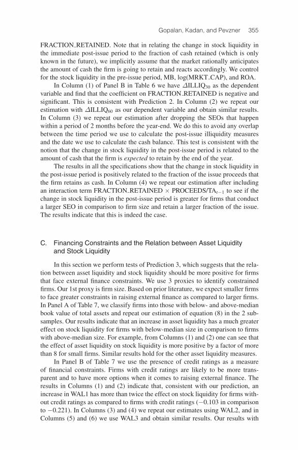
In this section we perform tests of Prediction 3, which suggests that the rela-tion between asset liquidity and stock liquidity should be more positive for firmsthat face external finance constraints. We use 3 proxies to identify constrainedfirms. Our 1st proxy is firm size. Based on prior literature, we expect smaller firmsto face greater constraints in raising external finance as compared to larger firms.In Panel A of Table 7, we classify firms into those with below- and above-medianbook value of total assets and repeat our estimation of equation (8) in the 2 sub-samples. Our results indicate that an increase in asset liquidity has a much greatereffect on stock liquidity for firms with below-median size in comparison to firmswith above-median size. For example, from Columns (1) and (2) one can see thatthe effect of asset liquidity on stock liquidity is more positive by a factor of morethan 8 for small firms. Similar results hold for the other asset liquidity measures.
In Panel B of Table 7 we use the presence of credit ratings as a measureof financial constraints. Firms with credit ratings are likely to be more trans-parent and to have more options when it comes to raising external finance. Theresults in Columns (1) and (2) indicate that, consistent with our prediction, anincrease in WAL1 has more than twice the effect on stock liquidity for firms with-out credit ratings as compared to firms with credit ratings (−0.103 in comparisonto −0.221). In Columns (3) and (4) we repeat our estimates using WAL2, and inColumns (5) and (6) we use WAL3 and obtain similar results. Our results with

356 Journal of Financial and Quantitative Analysis
TABLE 7
Asset Liquidity and Stock Liquidity
Panel A of Table 7 reports the results of the regression relating a firm’s asset liquidity to stock liquidity. Specifically, weestimate the panel OLS regression: Yi,t = α + βXi,t + γCONTROLSi,t + μi + μt + εi,t, where Yi,t is a measure of stockliquidity for firm i during year t, Xi,t is a measure of asset liquidity, μi are firm fixed effects, andμt are year dummy variables.Y is ILLIQ. In Panel A we estimate the regression in subsamples with above- and below-median book value of total assets.All variables are defined in Appendix B. To test if the coefficient on the measures of asset liquidity is significantly differentacross the 2 subsamples, we estimate a single equation with a full set of interaction terms between all independent variablesand a dummy variable that identifies firms with above-median book value of total assets and test if the coefficient on theasset liquidity interaction term is significantly different from 0. We present the results of the test in the row titled ΔCOEFF.The sample includes all firms with financial data in Compustat during the years 1962–2005. Panel B reports the results of theregression relating a firm’s asset liquidity to stock liquidity with the sample split into firms with and without short-term creditratings. The dependent variable is ILLIQ. All variables are defined in Appendix B. To test if the coefficient on the measuresof asset liquidity is significantly different across the 2 subsamples, we estimate a single equation with a full set of interactionterms between all independent variables and a dummy variable that identifies rated firms and test if the coefficient on theasset liquidity interaction term is significantly different from 0. We present the results of the test in the row titled ΔCOEFF.All variables are winsorized at the 1st and 99th percentiles. The sample includes all firms with financial data in Compustatduring the years 1962–2005. Panel C reports the results of the regression relating a firm’s asset liquidity to stock liquiditywith the sample split into firms with above- and below-median default probability. We measure default probability usingthe Bharath and Shumway (2008) methodology. The dependent variable is ILLIQ. All variables are defined in Appendix B.To test if the coefficient on the measures of asset liquidity is significantly different across the 2 subsamples, we estimate asingle equation with a full set of interaction terms between all independent variables and a dummy variable that identifiesfirms with above-median default likelihood and test if the coefficient on the asset liquidity interaction term is significantlydifferent from 0. We present the results of the test in the row titled ΔCOEFF. The sample includes all firms with financialdata in Compustat during the years 1970–2006. All variables are winsorized at the 1st and 99th percentiles. The standarderrors are clustered at the individual firm level. ***, **, and * denote statistical significance at the 1%, 5%, and 10% levels,respectively.
Panel A. Small versus Large Firms
Large Small Large Small Large Small Large Small
(1) (2) (3) (4) (5) (6) (7) (8)
WAL1 −0.031 −0.260(0.009)*** (0.022)***
WAL2 −0.059 −0.314(0.010)*** (0.020)***
WAL3 −0.037 −0.249(0.007)*** (0.015)***
MWAL −0.064 −0.400(0.014)*** (0.026)***
log(MRKT −0.071 −0.338 −0.072 −0.342 −0.072 −0.344 −0.077 −0.401CAP)t−1 (0.003)*** (0.007)*** (0.003)*** (0.007)*** (0.003)*** (0.007)*** (0.004)*** (0.009)***
No. of obs. 33,818 40,977 33,818 40,977 33,818 40,977 33,818 40,977R2 0.784 0.763 0.784 0.764 0.784 0.764 0.784 0.766
ΔCOEFF 0.229 0.255 0.212 0.336(0.024)*** (0.022)*** (0.017)*** (0.029)***
Panel B. Rated versus Unrated Firms
Rated Unrated Rated Unrated Rated Unrated Rated Unrated
(1) (2) (3) (4) (5) (6) (7) (8)
WAL1 −0.103 −0.221(0.027)*** (0.020)***
WAL2 −0.138 −0.275(0.022)*** (0.018)***
WAL3 −0.090 −0.212(0.015)*** (0.013)***
MWAL −0.235 −0.237(0.027)*** (0.022)***
log(MRKT −0.085 −0.260 −0.087 −0.264 −0.087 −0.264 −0.105 −0.291CAP)t−1 (0.007)*** (0.006)*** (0.007)*** (0.006)*** (0.007)*** (0.006)*** (0.008)*** (0.007)***
No. of obs. 14,629 60,166 14,629 60,166 14,629 60,166 14,629 60,166R2 0.809 0.779 0.81 0.78 0.81 0.78 0.813 0.78
ΔCOEFF 0.119 0.137 0.121 0.002(0.034)*** (0.028)*** (0.02)*** (0.035)
(continued on next page)
Gopalan, Kadan, and Pevzner 357
TABLE 7 (continued)
Asset Liquidity and Stock Liquidity
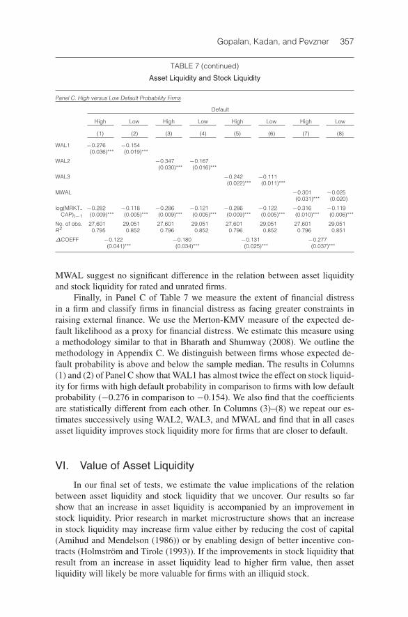
Panel C. High versus Low Default Probability Firms
Default
High Low High Low High Low High Low
(1) (2) (3) (4) (5) (6) (7) (8)
WAL1 −0.276 −0.154(0.036)*** (0.019)***
WAL2 −0.347 −0.167(0.030)*** (0.016)***
WAL3 −0.242 −0.111(0.022)*** (0.011)***
MWAL −0.301 −0.025(0.031)*** (0.020)
log(MRKT −0.282 −0.118 −0.286 −0.121 −0.286 −0.122 −0.316 −0.119CAP)t−1 (0.009)*** (0.005)*** (0.009)*** (0.005)*** (0.009)*** (0.005)*** (0.010)*** (0.006)***
No. of obs. 27,601 29,051 27,601 29,051 27,601 29,051 27,601 29,051R2 0.795 0.852 0.796 0.852 0.796 0.852 0.796 0.851
ΔCOEFF −0.122 −0.180 −0.131 −0.277(0.041)*** (0.034)*** (0.025)*** (0.037)***
MWAL suggest no significant difference in the relation between asset liquidityand stock liquidity for rated and unrated firms.
Finally, in Panel C of Table 7 we measure the extent of financial distressin a firm and classify firms in financial distress as facing greater constraints inraising external finance. We use the Merton-KMV measure of the expected de-fault likelihood as a proxy for financial distress. We estimate this measure usinga methodology similar to that in Bharath and Shumway (2008). We outline themethodology in Appendix C. We distinguish between firms whose expected de-fault probability is above and below the sample median. The results in Columns(1) and (2) of Panel C show that WAL1 has almost twice the effect on stock liquid-ity for firms with high default probability in comparison to firms with low defaultprobability (−0.276 in comparison to −0.154). We also find that the coefficientsare statistically different from each other. In Columns (3)–(8) we repeat our es-timates successively using WAL2, WAL3, and MWAL and find that in all casesasset liquidity improves stock liquidity more for firms that are closer to default.
VI. Value of Asset Liquidity
In our final set of tests, we estimate the value implications of the relationbetween asset liquidity and stock liquidity that we uncover. Our results so farshow that an increase in asset liquidity is accompanied by an improvement instock liquidity. Prior research in market microstructure shows that an increasein stock liquidity may increase firm value either by reducing the cost of capital(Amihud and Mendelson (1986)) or by enabling design of better incentive con-tracts (Holmstrom and Tirole (1993)). If the improvements in stock liquidity thatresult from an increase in asset liquidity lead to higher firm value, then assetliquidity will likely be more valuable for firms with an illiquid stock.
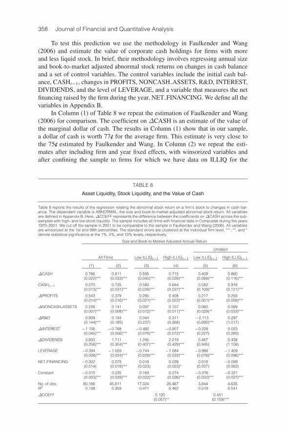
358 Journal of Financial and Quantitative Analysis
To test this prediction we use the methodology in Faulkender and Wang(2006) and estimate the value of corporate cash holdings for firms with moreand less liquid stock. In brief, their methodology involves regressing annual sizeand book-to-market adjusted abnormal stock returns on changes in cash balanceand a set of control variables. The control variables include the initial cash bal-ance, CASHt−1, changes in PROFITS, NONCASH ASSETS, R&D, INTEREST,DIVIDENDS, and the level of LEVERAGE, and a variable that measures the netfinancing raised by the firm during the year, NET FINANCING. We define all thevariables in Appendix B.
In Column (1) of Table 8 we repeat the estimation of Faulkender and Wang(2006) for comparison. The coefficient on ΔCASH is an estimate of the value ofthe marginal dollar of cash. The results in Column (1) show that in our sample,a dollar of cash is worth 77c/ for the average firm. This estimate is very close tothe 75c/ estimated by Faulkender and Wang. In Column (2) we repeat the esti-mates after including firm and year fixed effects, with winsorized variables andafter confining the sample to firms for which we have data on ILLIQ for the
TABLE 8
Asset Liquidity, Stock Liquidity, and the Value of Cash
Table 8 reports the results of the regression relating the abnormal stock return on a firm’s stock to changes in cash bal-ance. The dependent variable is ABNORMAL, the size and book-to-market adjusted abnormal stock return. All variablesare defined in Appendix B. Here,ΔCOEFF represents the difference between the coefficients onΔCASH across the sub-samples with high- and low-stock liquidity. The sample includes all firms with financial data in Compustat during the years1970–2001. We cut off the sample in 2001 to be comparable to the sample in Faulkender and Wang (2006). All variablesare winsorized at the 1st and 99th percentiles. The standard errors are clustered at the individual firm level. ***, **, and *denote statistical significance at the 1%, 5%, and 10% levels, respectively.
Size and Book-to-Market Adjusted Annual Return
Unrated
All Firms Low ILLIQt−1 High ILLIQt−1 Low ILLIQt−1 High ILLIQt−1
(1) (2) (3) (4) (5) (6)
ΔCASH 0.766 0.811 0.595 0.715 0.409 0.860(0.022)*** (0.033)*** (0.045)*** (0.039)*** (0.089)*** (0.116)***
CASHt−1 0.270 0.725 0.580 0.644 0.582 0.918(0.013)*** (0.031)*** (0.038)*** (0.037)*** (0.109)*** (0.121)***
ΔPROFITS 0.543 0.379 0.285 0.408 0.217 0.293(0.014)*** (0.016)*** (0.021)*** (0.022)*** (0.051)*** (0.058)***
ΔNONCASH ASSETS 0.226 0.141 0.097 0.157 0.060 0.089(0.007)*** (0.008)*** (0.012)*** (0.011)*** (0.029)** (0.033)***
ΔR&D 0.939 0.194 0.044 0.311 −2.113 0.297(0.144)*** (0.185) (0.237) (0.268) (0.695)*** (1.017)
ΔINTEREST −1.156 −0.768 −0.492 −0.807 −0.228 0.023(0.045)*** (0.056)*** (0.078)*** (0.072)*** (0.227) (0.260)
ΔDIVIDENDS 3.933 1.711 1.245 2.219 0.467 0.439(0.258)*** (0.304)*** (0.407)*** (0.429)*** (0.945) (1.108)
LEVERAGE −0.394 −1.059 −0.744 −1.084 −0.986 −1.409(0.008)*** (0.024)*** (0.028)*** (0.033)*** (0.076)*** (0.096)***
NET FINANCING −0.002 0.073 0.018 0.039 0.010 −0.099(0.014) (0.018)*** (0.023) (0.023)* (0.057) (0.062)
Constant −0.015 0.235 0.169 0.274 −0.376 −0.321(0.003)*** (0.029)*** (0.022)*** (0.026)*** (0.032)*** (0.027)***
No. of obs. 80,166 45,811 17,324 28,487 3,844 4,635R2 0.138 0.359 0.471 0.462 0.519 0.541
ΔCOEFF 0.120 0.451(0.057)** (0.159)***
Gopalan, Kadan, and Pevzner 359
previous year. We include the last criteria because the sample in the subsequentcolumns is confined to such firms. The results in Column (2) indicate that $1 ofcash is worth 81c/ on average. In Columns (3)–(4) we divide our sample into firmswith above- and below-median stock liquidity (as measured by ILLIQ) and repeatthe estimation in the 2 subsamples. Faulkender and Wang show that cash is morevaluable for smaller firms that may face greater external financial constraints.Since smaller firms are also likely to have illiquid stock, we need to control forfirm size in our estimation. We do this by dividing our sample into market capi-talization deciles and identifying high- and low-liquidity firms within the deciles.This ensures that the median market capitalization of firms in both the high- andlow-liquidity subsamples are the same. Our results in Columns (3)–(4) of Table 8show that consistent with our conjecture, an additional dollar of cash is morevaluable for firms with less liquid stock. The row titled ΔCOEFF indicates that adollar of cash is worth 12c/ more for firms with below-median stock liquidity.20 InColumns (5)–(6) we further control for access to external finance by limiting oursample to firms without long-term bond ratings. Our results again show that cashis more valuable for firms with below-median stock liquidity.
VII. Conclusion
In this paper we study the balance sheet of liquidity: the relation betweenthe liquidity of the firm’s assets and the liquidity of financial claims on the assets,thereby linking corporate finance decisions to stock liquidity. Our model high-lights that the relation may be either positive or negative depending on parametervalues. Greater asset liquidity reduces uncertainty regarding valuation of assets-in-place, but it also increases future investments and the associated uncertainty.The model departs from the perfect MM (1958) world by assuming that the sourceof capital affects investment decisions. As a result, the model shows that asset liq-uidity improves stock liquidity more for firms that are less likely to reinvest theirliquid assets: firms with less growth opportunities, financially constrained firms,and firms with low correlation between assets-in-place and new projects.
Empirically, we find a positive and economically large relation between assetliquidity and stock liquidity. Consistent with our model, the relation is more posi-tive for firms with low growth opportunities and for financially constrained firms.The results hold both in the time series and in the cross section, and are reinforcedby an event study.
The relation between asset liquidity and stock liquidity also has value im-plications. Indeed, the effect of a high cash balance in improving stock liquidityis a hitherto unknown benefit of cash. We find that an increase in corporate cashholding is significantly more valuable for firms with less liquid stock.
Finally, our analysis linking corporate finance to stock liquidity has furtherimplications, the empirical study of which is beyond the scope of this paper. Oneexample is the result that the relation between asset liquidity and stock liquid-ity is more positive for firms with low correlation between assets-in-place and
20In unreported tests we find our estimates robust to estimating a single regression on the fullsample with an interaction term, HIGH ILLIQ ×ΔCASH.
360 Journal of Financial and Quantitative Analysis
new projects. The 2nd example is commonality in stock liquidity. We show thatthe relation between asset liquidity and stock liquidity depends strongly on in-vestment opportunities. Such opportunities covary at the industry, economy, andglobal level. This suggests that stock liquidity may have a common componentnot only at the market level, but also at the industry and global levels. Anotherimplication is the long-term stock underperformance after firm financing. Theimprovement in stock liquidity following such financing (as highlighted by ourresults) is likely to reduce the liquidity risk premium for the stock, which in turnis likely to reflect as underperformance based on the ex ante risk characteristics.
Appendix A. Proofs
Proof of Proposition 1. Recall that λ is a measure of stock illiquidity. Thus, ∂λ/∂α ≤ 0means that higher asset liquidity is associated with higher stock liquidity. Differentiatingequation (6) with respect to α we have
∂λ
∂α=
12σu
∂σ20
∂α.(A-1)
Since σu > 0, ∂λ/∂α ≤ 0 is equivalent to ∂σ20/∂α ≤ 0. Differentiating equation (5) with
respect to α we obtain
∂σ20
∂α= −2 (1− α)σ2
x + 2αk2h (γ∗)2 σ2y + 2 (1− 2α) kh (γ∗)σxσyρ.(A-2)
Thus, ∂σ20/∂α ≤ 0 if and only if
α(σ2
x + k2h (γ∗)2 σ2y − 2kh (γ∗)σxσyρ
)≤ σ2
x − kh (γ∗)σxσyρ,
or21
α ≤ σ2x − kh (γ∗)σxσyρ
σ2x + k2h (γ∗)2 σ2
y − 2kh (γ∗)σxσyρ≡ α.
Proof of Proposition 2. Differentiating equation (A-2) with respect to k, we obtain
∂2σ20
∂k∂α= 4αkh (γ∗)2 σ2
y + 4αk2h (γ∗) h′ (γ∗)∂γ∗
∂k(A-3)
+ 2 (1− 2α)σxσyρ
(h (γ∗) + kh′ (γ∗)
dγ∗
dk
).
Using equation (4), this expression is clearly positive for α ≤ 1/2. Consequently,∂2λ/(∂k∂α) > 0. Since λ is a measure of stock illiquidity, this means that the relationbetween asset liquidity and stock liquidity is weaker (less positive or more negative) forfirms with higher values of k (higher growth opportunities).
Proof of Proposition 3. Since γ∗ is higher for an unconstrained firm and since h(·) is in-creasing in γ, the 2nd term in equation (A-2) is larger for an unconstrained firm as opposedto a constrained firm. Similarly, since α ≤ 0.5, and ρ ≥ 0, the 3rd term is also larger for
21Note that
σ2x + k2h (γ∗)2 σ2
y − 2kh (γ∗)σxσyρ > 0,
and hence dividing by this term does not reverse the inequality.

Gopalan, Kadan, and Pevzner 361
an unconstrained firm. Hence, ∂σ20/∂α is smaller for a constrained firm as compared to an
unconstrained firm.
Proof of Proposition 4. Differentiating equation (A-2) with respect to ρ, we obtain
∂2σ20
∂ρ∂α= 2 (1− 2α) kh (γ∗)σxσy.(A-4)
Thus, (∂2σ20)/(∂ρ∂α) is clearly positive (negative) for α < 0.5 (α > 0.5).
Appendix B. Description of Variables
ABNORMAL: Size and book-to-market adjusted abnormal stock return.
BHAR: Buy-and-hold annual abnormal stock return. It is the difference between the annualreturn on the firm’s stock and the return on the value-weighted portfolio of all NYSE,AMEX, and NASDAQ stocks.
CAPEX: Ratio of a firm’s capital expenditures (Data128) to lagged total assets (Data6).When Data128 is missing, this variable is set to 0.
CASH: Ratio of book value of cash over lagged market value of equity.
DEF PROB: Expected default probability estimated using the approach in Bharath andShumway (2008) (see Appendix C).
ΔCASH: Ratio of change in the book value of cash over lagged market value of equity.
ΔDIVIDENDS: Ratio of change in dividends over lagged market value of equity.
ΔINTEREST: Ratio of change in interest expense over lagged market value of equity.
ΔNONCASH ASSETS: Ratio of change in net assets, which is the difference betweenbook value of total assets and book value of cash over lagged market value of equity.
ΔPROFITS: Ratio of change in operating profits over lagged market value of equity.
ΔR&D: Ratio of change in R&D expenditure over lagged market value of equity.
DISC ACC: Measure of a firm’s abnormal accruals originally proposed in Jones (1991)and modified to control for performance per Kothari, Leone, and Wasley (2005).
FRACTION RETAINED: Ratio of the change in cash balance between the year endingafter the SEO to the year ending before the SEO deflated by the size of the SEO.
ILLIQ: Square root of average annual Amihud (2002) illiquidity measure. Amihud’s mea-sure is the ratio of the absolute daily stock return and the daily dollar volume. Data forthis variable were obtained from Hasbrouck’s Web site (http://people.stern.nyu.edu/jhasbrou/ ).
ILLIQ−30,0: Average ILLIQ over the 30 trading days prior to the SEO.
ILLIQ−60,0: Average ILLIQ over the 60 trading days prior to the SEO.
ILLIQ15,45: Average ILLIQ over the period of 15–45 trading days following the SEO.
ILLIQ15,75: Average ILLIQ over the period of 15–75 trading days following the SEO.
LEVERAGE: Book value of long- and short-term debt over lagged market value of equity.
log(MRKT CAP): Natural log of a firm’s market value of equity (Data25 × Data199).
MB: The ratio of market value of equity to book value of equity.
MWAL: Ratio of the sum of cash, 0.75 × the value of noncash current assets and 0.5 ×the value of other tangible fixed assets, to lagged market value of total assets. Wecalculate market value of total assets as the sum of book value of total assets andmarket value of equity less book value of equity.
NET FINANCING: Ratio of net financing, which is the sum of equity issued and long-term debt issued less shares repurchased and long-term debt repurchased over laggedmarket value of equity.
362 Journal of Financial and Quantitative Analysis
PROCEEDS/TA: The ratio of SEO proceeds to lagged book value of total assets.
PS-GAMMA: Annual Pastor and Stambaugh (2003) gamma coefficient obtained fromHasbrouck’s Web site (http://people.stern.nyu.edu/jhasbrou/).
s: Gibbs sampler estimate of Roll’s (1984) implicit measure of trading costs. Data for thisvariable were also obtained from Hasbrouck’s Web site (http://people.stern.nyu.edu/jhasbrou/ ).
RATED: A dummy variable that identifies firms with nonmissing S&P long-term creditratings in Compustat.
ROA: Ratio of earnings before depreciation, interest, and taxes over lagged value of totalassets.
SPREAD: Average intraday daily effective percentage bid-ask spread estimated from TAQ.The data on the effective spread were obtained from the Web site of the Universityof Vanderbilt’s Financial Markets Research Center (http://www.vanderbiltfmrc.org/)and are available only for the subperiod 1993–2003.
WAL1: Ratio of the sum of cash and cash equivalents to lagged value of total assets.
WAL2: Ratio of the sum of cash and 0.5 × the value of noncash current assets, to laggedvalue of total assets.
WAL3: Ratio of the sum of cash, 0.75 × the value of noncash current assets and 0.5 × thevalue of other tangible fixed assets, to lagged value of total assets.
VOLATILITY: Standard deviation of a firm’s stock returns over the 60 months precedingthe beginning of a current fiscal year.
Appendix C. Details of the Calculation of the ModifiedMerton-KMV Default Probability
We calculate the expected default probability using the modified Merton-KMV pro-cedure. This involves viewing the firm’s equity as a call option on the underlying assetswith a strike price equal to the book value of total debt. We use the Black-Scholes (1973)option pricing formula for European call options to estimate the default probability. Thekey parameters required to calculate the default probability are listed below. We first pro-pose an initial value of the volatility of the firm’s assets, σV , and use it along with the bookvalue of total debt F, the market value of total assets V (the sum of the market value ofequity and the book value of debt), and the risk-free rate r and apply equation (C-1) to inferthe market value of the firm’s equity, E. We use the market value of the firm’s equity alongwith the book value of total debt to estimate the market value of the firm’s total assets atthe end of every day during the previous year. We use these market values to calculate thelog return on assets each day and use the return series to generate a new estimate for thevolatility of the assets, σV , and the expected return on the assets, μ. We iterate on σV in thismanner until it converges (so the absolute difference in adjacent σV s is less than 10−3). Wethen calculate the expected default probability, DEF PROB using equation (C-3).
E = V N(d1)− e−rT FN(d2),(C-1)
where E is the market value of the firm’s equity and
d1 =ln(V/F) +
(r + 0.5σ2
V
)T
σV
√T
,(C-2)
and d2 is just d1 − σV
√T .
DEF PROB = N
(−(
ln(V/F) +(μ− 0.5σ2
V
)T
σV
√T
)).(C-3)
Gopalan, Kadan, and Pevzner 363
σV : Volatility of the firm’s assets.
μ: Expected return on the firm’s assets.
F: Book value of total debt.
r: Risk-free rate.
V: Market value of total assets.
T: Time to maturity (1 year).
E: Market value of the firm’s equity.
ReferencesAmihud, Y. “Illiquidity and Stock Returns: Cross-Section and Time-Series Effects.” Journal of Finan-
cial Markets, 5 (2002), 31–56.Amihud, Y., and H. Mendelson. “Asset Pricing and the Bid-Ask Spread.” Journal of Financial Eco-
nomics, 17 (1986), 223–249.Arellano, M., and S. Bond. “Some Tests of Specification for Panel Data: Monte Carlo Evidence and
an Application to Employment Equations.” Review of Economic Studies, 58 (1991), 277–297.Berger, A. N., and C. H. S. Bouwman. “Bank Liquidity Creation.” Review of Financial Studies,
22 (2009), 3779–3837.Bharath, S. T., and T. Shumway. “Forecasting Default with the Merton Distance-to-Default Model.”
Review of Financial Studies, 21 (2008), 1339–1369.Bhattacharya, N.; H. Desai; and K. Venkataraman. “Earnings Quality and Information Asymmetry:
Evidence from Trading Costs.” Working Paper, Southern Methodist University (2007).Black, F., and M. Scholes. “The Pricing of Options and Corporate Liabilities.” Journal of Political
Economy, 81 (1973), 637–654.Boehmer, E.; C. Jones; and X. Zhang. “Shackling Short Sellers: The 2008 Shorting Ban.” Working
Paper (2009). Available at SSRN: http://ssrn.com/abstract=1412844.Chordia, T.; R. Roll; and A. Subrahmanyam. “Why Has Trading Volume Increased?” Working Paper,
University of California at Los Angeles (2007).Cooper, M. J.; H. Gulen; and M. J. Schill. “Asset Growth and the Cross-Section of Stock Returns.”
Journal of Finance, 63 (2008), 1609–1651.DeAngelo, H.; L. DeAngelo; and K. H. Wruck. “Asset Liquidity, Debt Covenants, and Managerial
Discretion in Financial Distress: The Collapse of L.A. Gear.” Journal of Financial Economics,64 (2002), 3–34.
Diamond, D. W., and R. E. Verrecchia. “Disclosure, Liquidity, and the Cost of Capital.” Journalof Finance, 46 (1991), 1325–1359.
Eckbo B. E.; R. W. Masulis; and O. Norli. “Seasoned Public Offerings: Resolution of the ‘New IssuesPuzzle’.” Journal of Financial Economics, 56 (2000), 251–291.
Fama, E. F., and K. R. French. “Testing Tradeoff and Pecking Order Predictions about Dividends andDebt.” Review of Financial Studies, 15 (2002), 1–33.
Fama, E., and J. MacBeth. “Risk, Return, and Equilibrium: Empirical Tests.” Journal of PoliticalEconomy, 81 (1973), 607–636.
Faulkender, M., and R. Wang. “Corporate Financial Policy and the Value of Cash.” Journal of Finance,61 (2006), 1957–1990.
Foley, C. F.; J. C. Hartzell; S. Titman; and G. Twite. “Why Do Firms Hold So Much Cash? A Tax-Based Explanation.” Journal of Financial Economics, 86 (2007), 579–607.
Hasbrouck, J. “Trading Costs and Returns for U.S. Equities: Estimating Effective Costs from DailyData.” Journal of Finance, 64 (2009), 1445–1477.
Holmstrom, B., and J. Tirole. “Market Liquidity and Performance Monitoring.” Journal of PoliticalEconomy, 101 (1993), 678–709.
Jones, J. J. “Earnings Management during Import Relief Investigations.” Journal of AccountingResearch, 29 (1991), 193–228.
Keynes, J. Treatise on Money. London: Macmillan (1930).Kothari, S. P.; A. J. Leone; and C. E. Wasley. “Performance Matched Discretionary Accrual Mea-
sures.” Journal of Accounting and Economics, 39 (2005), 163–197.Kyle, A. S. “Continuous Auction and Insider Trading.” Econometrica, 53 (1985), 1315–1336.Lesmond, D. A.; J. P. Ogden; and C. A. Trzcinka. “A New Estimate of Transaction Costs.” Review
of Financial Studies, 12 (1999), 1113–1141.

364 Journal of Financial and Quantitative Analysis
Miller, M. H., and K. Rock. “Dividend Policy under Asymmetric Information.” Journal of Finance,40 (1985), 1031–1051.
Modigliani, F., and M. H. Miller. “The Cost of Capital, Corporation Finance and the Theory of Invest-ment.” American Economic Review, 48 (1958), 261–297.
Myers, S. C. “Determinants of Corporate Borrowing.” Journal of Financial Economics, 5 (1977),147–175.
Pastor, L., and R. F. Stambaugh. “Liquidity Risk and Expected Stock Returns.” Journal of PoliticalEconomy, 111 (2003), 642–685.
Roll, R. “A Simple Implicit Measure of the Effective Bid-Ask Spread in an Efficient Market.” Journalof Finance, 39 (1984), 1127–1139.