Copyright

by

Aditya Gopalan

2011

The Dissertation Committee for Aditya Gopalancertifies that this is the approved version of the following dissertation:

Wireless Scheduling with Limited Information

Committee:

Sanjay Shakkottai, Supervisor

Constantine Caramanis, Co-Supervisor

Jeffrey Andrews

Gustavo de Veciana

David Morton

Sujay Sanghavi

Wireless Scheduling with Limited Information

by

Aditya Gopalan, B.Tech., M.Tech.

Dissertation

Presented to the Faculty of the Graduate School of

The University of Texas at Austin

in Partial Fulfillment

of the Requirements

for the Degree of

Doctor of Philosophy

The University of Texas at Austin

December 2011

To my parents.

Acknowledgments

My time spent in graduate school has, without doubt, been immensely sat-

isfying. I look back upon it as a journey of learning and discovery in innumerable

ways, an experience that would be impossible without the support and encourage-

ment of many people around me. I am grateful, and remain indebted, to all of them

for what I have learnt.

As my academic foster-parents, my advisors Sanjay and Constantine have

brought me up from a fledgling student to an able researcher. Sanjay has never

ceased to inspire me with his unending passion for research,his infectious enthusi-

asm to both teach and absorb, and the constant care for his students. His guidance

has been well-complemented by Constantine’s invaluable mentorship. Constan-

tine’s doors have always been open to me in times of confusionand struggle, and I

cannot forget the countless hours spent with him discussingresearch problems and

future avenues. He has been instrumental in broadening my research horizons, to

help me bridge across research areas to machine learning andoptimization. I cannot

thank Sanjay and Constantine enough for their teachings.

I am grateful to my committee members for their honest appraisal of my

dissertation, and for their valuable feedback on several aspects of it. In addition,

I have had the privilege of being taught by several exemplaryprofessors during

my stint here at UT, such as Gordan Zitkovic, Greg Plaxton, David Zuckerman,

Gustavo de Veciana, David Morton, Adam Klivans, Hans Koch, P. Souganidis and

John Tate. Much of my formative years as a graduate student have been shaped by

their teaching experiences, for which I am thankful.

v

It is only my good fortune to have had the dynamic working environment

of the Wireless Networking and Communications Group at UT. I have greatly ben-

efited technically from the excellent company of my peers at WNCG, and it has

always been a pleasure to sharpen knives together – by way of attending seminars,

discussing research problems and puzzles. In this regard, Icannot forget the times

spent with Shreeshankar Bodas, Siddhartha Banerjee, Aneesh Reddy, Sundar Sub-

ramanian, Raghu Meka, Sandeep Bhadra, Kumar Appaiah, Zrinka Puljiz, Ali Jalali,

Jubin Jose, Rahul Vaze, Harish Ganapathy, Sriram Sridharan,Ioannis Mitliagkas,

Abhik Das and Praneeth Netrapalli, among others. May the tribe increase!

For administrative work at UT, which usually goes unnoticedbehind the

scenes, I cannot forget gracious help from the WNCG staff – Lori Lacy, Wanda

Franklin, Janet Preuss, Paul White, Jocelyn Charvet and Jennifer Graham – that

ensured, among many other things, that my tuition was paid and I received my

monthly stipend on time!

The friendships I have forged here at UT have enriched my staybeyond

measure. I greatly appreciate the moments spent with each ofmy friends here,

many of which have opened my eyes to the warmth of human bonding. I confess

that my abilities are inadequate to express all that I feel for them.

I have been deeply touched in the course of my close friendship with Shweta

Agrawal, and cannot thank her enough for what our association has meant to me.

With her constant love, affection and concern for my welfare, she has been no less

than family, and I can only be grateful that fate caused our paths to meet.

I have had the pleasure of living with my wonderful friend androommate

Shivaram Kalyanakrishnan for all five years of my graduate stay in Austin. It is

not without reason that our domestic partnership has been light-heartedly likened

vi

to husband and wife! Jokes apart, Shiva has been a pillar of support just with his

presence throughout, and I wish him the best for his life ahead.

My dear friends – Zrinka Puljiz, Petar Buva, Siddhartha Banerjee, Richa

Sardana, Meghana Deodhar, Harish Ganapathy, Amitanand Aiyer, Raghu Meka,

Sunil Kowlgi, Ranga Vasudevan, Radhakrishna BR, Vaidyanathan Krishnamurthy,

Shreeshankar Bodas, Bharath Balasubramanian, Smita Naik, Rohan Joseph, Suriya

Subramanian, Shobha Sundar Ram, among many others – have stayed with me

through thick and thin, and my extended fruitful interactions with them remain a

source of joy and encouragement.

Above all, the seeds of this undertaking would not have been sown without

my family’s encouragement and wishes from back home. I am still at a loss to un-

derstand how Amma and Dad could be sources of unending strength from halfway

across the world in India. I owe my deepest gratitude to them for their presence

in my world, whether it be during dark hours or moments of joy.The complete

freedom that they have accorded me in following my interestsis something I have

grown to cherish and respect. Anu, Avva and both my Thathas, along with my dear

Vijaya aunty, have been well-wishers throughout, and for this I remain thankful to

them.

vii

Wireless Scheduling with Limited Information

Aditya Gopalan, Ph.D.

The University of Texas at Austin, 2011

Supervisors: Sanjay ShakkottaiConstantine Caramanis

This thesis examines the problem of scheduling with incomplete and/or lo-

cal information in wireless systems. With large numbers of users and limited feed-

back resources, wireless systems require good scheduling algorithms to attain their

performance limits. Classical studies on wireless scheduling investigate in much

detail settings where the full state of the system is available when scheduling users.

In contrast, this thesis focuses on the case where valuable network state information

is lacking at the scheduler, and studies its resulting effect on system performance.

The insights gained from the analysis are used to develop efficient wireless schedul-

ing algorithms that operate with limited state information, and that guarantee high

throughput and delay performance.

The first part of the thesis considers scheduling for stability in a wireless

downlink system, where a base station or server schedules transmissions to users,

while acquiring channel state information from only subsets of users. It is shown

that the system’s throughput region is completely characterized by the marginal

channel statistics over observable channel subsets. Effective, queue-length based

joint sampling and scheduling algorithms are developed that observe appropriate

subsets of channels and schedule users, and the algorithms are shown to be optimal

in the sense of throughput.

viii

Next, the thesis studies the queue-length performance of wireless schedul-

ing algorithms that use only partial, subset-based channelstate information. The

chief objective here is to design partial information-based scheduling algorithms

that keep the packet queues in the system short, and in this regard, the contributions

of this thesis are twofold. First, from the algorithmic perspective, wireless schedul-

ing algorithms using partial channel state information aredesigned that minimize

the likelihood of queue overflow, in a suitable sense, acrossall partial information

scheduling algorithms. The second key contribution is technical, by the develop-

ment of novel analytical techniques to study the stochasticdynamics of partial state

information-based algorithms. These techniques are not only instrumental in show-

ing the optimality results above, but are also of independent interest in understand-

ing the behavior of algorithms which rely on partially sampled system state.

The second part of the thesis investigates coordinated inter-cell wireless

scheduling across multiple base stations, each possessingonly local and partial

channel state information for its own users. Coordinated scheduling is necessary

to mitigate interference between users in adjacent cells, but information sharing

between the base stations is limited by high latencies in thebackhauls that inter-

connect them. A class of distributed scheduling algorithmsis developed in which

the base stations share only delayed queue length information with each other, and

locally acquire partial channel state information, to schedule users. These algo-

rithms are shown to be throughput-optimal, and their average backlog performance

in terms of the inter-base station latency is quantified.

ix

Table of Contents

Acknowledgments v

Abstract viii

List of Tables xii

List of Figures xiii

Chapter 1. Introduction 11.1 Overview . . . . . . . . . . . . . . . . . . . . . . . . . . . . . . . . 11.2 Contributions of this Thesis . . . . . . . . . . . . . . . . . . . . . . 51.3 Related Work . . . . . . . . . . . . . . . . . . . . . . . . . . . . . 7

Chapter 2. Downlink Scheduling: Stability and Throughput 152.1 Introduction . . . . . . . . . . . . . . . . . . . . . . . . . . . . . . 152.2 System Model . . . . . . . . . . . . . . . . . . . . . . . . . . . . . 192.3 Characterizing the Achievable Rate Region . . . . . . . . . . . . . .262.4 A Throughput-Optimal Scheduling Algorithm . . . . . . . . . .. . 402.5 The Max-Sum-Queue Algorithm . . . . . . . . . . . . . . . . . . . 422.6 Max-Sum-Queue applied to arbitrary subsets . . . . . . . . . .. . . 462.7 Conclusions and Future Work . . . . . . . . . . . . . . . . . . . . . 49

Chapter 3. Downlink Scheduling: Buffer Overflow Performance 513.1 Introduction . . . . . . . . . . . . . . . . . . . . . . . . . . . . . . 513.2 System Model . . . . . . . . . . . . . . . . . . . . . . . . . . . . . 553.3 Objective, Algorithms and Main Results . . . . . . . . . . . . . . .573.4 Sample Path Large Deviations Framework . . . . . . . . . . . . . .613.5 Analysis: Singleton Subsets and the Max-Queue Algorithm . . . . . 633.6 Analysis: General Subsets and the Max-Exp Algorithm . . .. . . . 723.7 Conclusions and Future Work . . . . . . . . . . . . . . . . . . . . . 87

x

Chapter 4. Coordinated Multi-cell Wireless Scheduling 884.1 Introduction . . . . . . . . . . . . . . . . . . . . . . . . . . . . . . 88

4.2 Motivating Example: How Throughput depends on the Coordina-tion Timescale . . . . . . . . . . . . . . . . . . . . . . . . . . . . . 92

4.3 System Model . . . . . . . . . . . . . . . . . . . . . . . . . . . . . 95

4.4 The Stability Region with Slow Global Coordination . . . . . .. . . 101

4.5 Throughput-optimal Scheduling with Slow Global Coordination . . . 108

4.6 Simulation Results: Impact ofT on Packet Delays underPT . . . . . 113

4.7 Conclusions and Future Work . . . . . . . . . . . . . . . . . . . . . 114

Chapter 5. Conclusions 117

Appendices 119

Appendix A. Proofs for Chapter 2 120A.1 Proof of Lemma 2.3 . . . . . . . . . . . . . . . . . . . . . . . . . . 120

A.2 Proof of Theorem 2.2 . . . . . . . . . . . . . . . . . . . . . . . . . 122

A.3 Proof of Lemma 2.4 . . . . . . . . . . . . . . . . . . . . . . . . . . 124

A.4 Proofs of Lemmas 2.5 and 2.6 . . . . . . . . . . . . . . . . . . . . . 126

A.5 Proof of Theorem 2.5 . . . . . . . . . . . . . . . . . . . . . . . . . 135

A.6 Proof of Theorem 2.6 . . . . . . . . . . . . . . . . . . . . . . . . . 136

Appendix B. Proofs for Chapter 3 145B.1 Proof of Proposition 3.1 . . . . . . . . . . . . . . . . . . . . . . . . 145

B.2 Proof of Proposition 3.3 . . . . . . . . . . . . . . . . . . . . . . . . 151

B.3 Proof of Proposition 3.4 . . . . . . . . . . . . . . . . . . . . . . . . 159

Appendix C. Proofs for Chapter 4 165C.1 Proof of Theorem 4.1 . . . . . . . . . . . . . . . . . . . . . . . . . 165

C.2 Proof of Theorem 4.2 . . . . . . . . . . . . . . . . . . . . . . . . . 167

Bibliography 173

Vita 188

xi

List of Tables

2.1 Probability assignments for three-channel system in Example 2.3.2 . 33

4.1 Channel state distribution for Three-user, Two-base-station systemexample . . . . . . . . . . . . . . . . . . . . . . . . . . . . . . . . 106

xii

List of Figures

2.1 Rate region for 3 channels with complete channel state information . 33

2.2 Rate region for 2 channelsci andcj, with complete channel stateinformation . . . . . . . . . . . . . . . . . . . . . . . . . . . . . . 34

2.3 Rate region for 3 channels with pairwise and singleton channel stateinformation . . . . . . . . . . . . . . . . . . . . . . . . . . . . . . 34

2.4 (a) Rate region with singleton channel state informationfor 2 chan-nels, (b) Rate region with full channel state information forjointdistributionπ(1), (c) Rate region with full channel state informationfor joint distributionπ(2). . . . . . . . . . . . . . . . . . . . . . . . 39

2.5 Rate region for described 3-channel system . . . . . . . . . . . .. 47

4.1 Throughput region for a 2-base station, 2-user system under schedul-ing with different information structures . . . . . . . . . . . . . . . 92

4.2 Coordinated scheduling model across multiple base stations withlocal information . . . . . . . . . . . . . . . . . . . . . . . . . . . 95

4.3 Stability region example: Three-user, Two-base-station System withslow coordination between the base stations . . . . . . . . . . . . .105

4.4 (a) Stability region for usersu1 and u2, (b) Stability region forusersu1 andu3, (c) Stability region for all three users . . . . . . . 107

4.5 Plot of average packet delay with lagT for various loads . . . . . . 115

4.6 Plot of average packet delay with load for various lagsT . . . . . . 116

xiii

Chapter 1

Introduction

1.1 Overview

Modern-day cellular networks handle steadily increasing amounts of data

with growing numbers of subscribers. Current estimates indicate that mobile data

traffic is growing by over 100% annually, with the trend projected to continue well

into the future [43]. Next-generation wireless standards such as Long Term Evolu-

tion (LTE) [68] and Worldwide Interoperability for Microwave Access (WiMAX)

[3] have been developed to be able to accommodate a wide variety of high-speed

applications over wireless, such as rapid file transfers, peer-to-peer sharing, online

gaming and real-time audio/video streaming. Supporting these applications over

many users, while maintaining an acceptable quality of service, imposes high per-

formance requirements on today’s wireless networks.

Several notions of performance exist for wireless systems.A prime perfor-

mance objective in a network is to maximizethroughput, i.e., the rates at which

data is communicated to and from users. Another important performance metric is

delaysincurred in data transmission, which is the time taken for data to travel from

source to destination. Packet delays play a critical role inthe quality of service

that users ultimately experience. It is highly desirable tohave as low packet delays

as possible in the network. This is because many applications such as real-time

audio/video and gaming impose stringent delay requirements on their data flows in

order to deliver a satisfactory user experience. Similarly, it is often desirable to keep

1

the likelihood of buffer overflow within the network down to a minimum, since this

directly affects in-network congestion and end-to-end delay performance. Other

metrics for quantifying network performance includefairnessacross users/flows,

and general notions of users’utilities, which could depend on other specific metrics

like rate or delay.

Engineering high-performance wireless networks warrantseffective resource

management. Available resources in multi-user wireless systems such as transmis-

sion/feedback bandwidth, capacity and time are limited. As a result, a key aspect of

network design is how to carefully apportion resources within the network in order

to meet performance demands. Modern wireless technology has evolved to make

dynamicresource allocation possible, meaning that resources suchas bandwidth

and frequency can be redistributed rapidly to take advantage of changing network

conditions.

Scheduling is the key function, within a wireless system, ofdynamically

assigning available system resources to users depending onuser requirements, and

using the degrees of flexibility provided by the system. Scheduling is a critical

component in the operation of a wireless system, because a significant part of over-

all system performance is directly influenced by how scheduling is performed at

its core. Hence, the design ofopportunistic schedulingalgorithms, to best exploit

network conditions, allocate resources and enable wireless systems to perform op-

timally, is of prime importance.

Through effective resource allocation, scheduling helps to overcome detri-

mental effects such as channel fading and interference, caused due to the physical

nature of the wireless medium. Multi-path propagation and reflection from ob-

stacles in the environment result in fading, i.e., time-varying fluctuations in sig-

nal quality. Transmitting information reliably and at highrates over time-varying

2

channels necessitates knowing the channel quality or statein advance. Recent de-

velopments in wireless technology, in modern systems such as LTE and WiMAX,

permit estimates of channel state from users to be fed back totransmitting base

stations (roughly, on the time scale of once every 1-2 milliseconds [113]). This

channel state feedback helps opportunistic scheduling algorithms at base stations

decide appropriate rate allocations to users, depending ontheir instantaneous chan-

nel qualities. For instance, users with better channels canhave more data scheduled

to them and vice versa, or when bandwidth is limited, only transmissions to users

with the best channels can be scheduled, etc.

However, in situations with a growing or excessive number ofusers, feed-

back bandwidth available in the wireless system is inadequate. This renders schemes

where a base station receives channel state feedback from all users untenable. To

mitigate this insufficiency, the base station might restrict itself to using onlypartial

Channel State Information (CSI), i.e., it might request channel state information

from only asub-collectionof channels, and perform scheduling based on this par-

tial CSI. It is important to understand scheduling with partial CSI in order to design

scheduling algorithms that use partial CSI from subsets of users and that can also

deliver high throughput/delay performance.

Scheduling across multiple cells or base stations brings its own set of chal-

lenges. Wireless transmissions to users in multicellular systems are prone to inter-

ference from those in nearby cells. Interference reduces the effective signal-to-noise

ratio at receivers and negatively impacts system performance, since little or no data

is transmitted when users’ transmissions interfere and collide. Thus, controlling in-

terference among users is important, in addition to overcoming the effects of chan-

nel fading. The effects of inter-cellular interference can be especially pronounced

in modern, fourth generation systems based on an OrthogonalFrequency Division

3

Multiple Access (OFDM) physical layer [106]. In such systems, each cell’s base

station allots non-interferingsub-channelsor frequencies to its users for transmis-

sion. However, users in adjacent cells, or those close to cell edges, that are assigned

similar frequencies collide to result in a loss of throughput. LTE-basedfemtocell

networks [55], consisting of mini base stations deployed inhome/office environ-

ments to improve coverage and/or rates, also suffer widely from interference – both

from neighboring base stations and macrocells.

Static frequency planning across multiple base stations can potentially re-

duce interference between such users located at the cell edges. Yet, with a large

number of users and/or a small set of sub-channels, a significant amount of inter-

ference may persist between users that are assigned the samefrequencies.

Inter-cellular interference can be alleviated in modern wireless systems us-

ing signaling capabilities provided via abackhaul– a common backbone connect-

ing the base stations together, which the base stations can use tocoordinatetheir

scheduling. This ensures that interfering users belongingto nearby cells at cell

edges are not scheduled together, helping to improve overall data rates. However,

avoiding such collisions entirely requiresfull coordinationusing complete, instan-

taneous CSI across all the base stations. Such coordination at the time-scale of

the channel fluctuations (i.e., about once every 1-2 ms) is infeasible due to the

relatively highlatenciesof the backhaul links – IP/Ethernet-based backhauls that

typically form the backbones of cellular/femtocell networks have latencies of the

order of tens to hundreds of ms [41, 56]. Information that canbe shared across the

base stations is delayed significantly from channel state variations, thus limiting the

amount of scheduling coordination between the base stations.

The goal of maximizing performance in a multiple base station scenario,

with partial CSI, inter-cellular interference and limited coordination, gives rise to

4

a challenging scheduling problem. The key objective here isto effectively use a

combination of (a) local, partial CSI at base stations, and (b) global, slower/delayed

information suitably shared across base stations, to schedule users in a distributed

fashion for high throughput.

1.2 Contributions of this Thesis

This thesis examines the problem of maximizing wireless network perfor-

mance under incomplete state information, from the point ofview of designing

scheduling algorithms. In this regard, the thesis developswireless scheduling algo-

rithms that acquire and use partial network state information from subsets of users,

and that, in many of the above general settings, enjoy high performance guarantees.

This thesis also introduces new analytical techniques which enable us to study the

performance of scheduling algorithms that use partial state information. Specifi-

cally, its contributions include:

• Throughput-optimal wireless scheduling with subset-based partial channel

state information (Chapter 2):When a base station can use channel state in-

formation from only chosen subsets of users, it is shown thatthe capacity or

throughput region of such a system is completely characterized by marginal

statistics of the channels over observable user subsets. A general schedul-

ing algorithm that picks subsets to observe depending on thequeue lengths

and expected channel rates of users, and that schedules using theMax-Weight

rule [4, 98], is shown to be throughput-optimal. For cases where the observ-

able collection of users is structured, e.g. disjoint or symmetric, this leads to

a much simpler scheduling algorithm calledMax-Sum-Queue, requiring no

statistical information at all, which is throughput-optimal.

5

• Low-delay scheduling with subset-based partial channel state information

(Chapter 3): We again consider a wireless downlink where a base station

schedules users using partial CSI from subsets of channels. Viewing the

system queue lengths as a surrogate for packet delays, we develop schedul-

ing algorithms that use only partial service rate information from subsets of

channels, and that minimize the likelihood of queue overflowin the system.

Specifically, we present a new joint subset-sampling and scheduling algo-

rithm calledMax-Expthat uses only the current queue lengths to pick a sub-

set of flows, and subsequently schedules a flow using the Exponential rule.

When the collection of observable subsets is disjoint, we show that Max-Exp

achieves the best exponential decay rate of the tail of the longest queue in the

system, among all scheduling algorithms using partial information.

To accomplish this, we introduce novel analytical techniques for studying the

performance of scheduling algorithms using partial state information, that are

of independent interest. These include new sample-path large deviations re-

sults for processes obtained by deterministic and predictable sampling of se-

quences of independent and identically distributed randomvariables, which

show that scheduling with partial state information yieldsa rate function sig-

nificantly different from the case of full information. As a special case, Max-

Exp reduces to simply serving the flow with the longest queue when the ob-

servable subsets are singleton flows, i.e., when there is effectively noa priori

channel-state information; thus, our results show that this greedy scheduling

policy is large-deviations optimal.

• Throughput-optimal multi-cell coordinated wireless scheduling with coordi-

nation latency (Chapter 4):We consider scheduling across multiple base sta-

tions, with each base station serving an exclusive set of users. Transmissions

6

to interfering users collide if scheduled simultaneously,and latency in the

inter-base station backhauls prohibits sharing instantaneous channel state in-

formation among base stations for coordination. In every time slot, each

base station picks asubsetof its users and observes instantaneous channel

states for those users in every time slot (thus, the base station haspartial

local channel state), and, together with globally delayed shared information

(e.g., delayed queue length state, channel statistics) from other base stations,

schedules users in the subset.

The throughput region of the network under such a scenario ischaracterized.

Using the key observation that common state information provided by global

delayed queues allows coupling of decisions, the optimal way of using this

coupled state in a multi-base-station scenario is demonstrated, and used to

develop a provably throughput-optimal scheduling algorithm. This is the first

throughput-optimality result using the information structure of local, limited

instantaneous channel state and global delayed queue lengths. The packet

delay performance of such an algorithm is also quantified, interms of the

amount of delay in the shared queue length information, by way of analysis

and simulations.

1.3 Related Work

Scheduling for wireless systems has been a well-studied topic of research

through the past few decades. A diverse body of work has been devoted to the devel-

opment of opportunistic wireless scheduling, in which knowledge of channel state

at the transmitter or base station is dynamically used for achieving higher perfor-

mance. This includes the basic approach of exploiting multi-user diversity, where

users with the best channel rates are favored to increase overall system through-

7

put [104, 111]. Several opportunistic scheduling techniques lend themselves to

optimization-based interpretations, and can be seen maximizing appropriate aggre-

gate utility functions across the system. Notable among these are Proportional-

Fair (PF) scheduling [1, 50, 51] that optimizes aggregate logarithmic utility, and

schemes to maximize weighted sum-rate with complete channel state information

[42].

The above methods largely rely on perfect channel state feedback from all

users, which could be prohibitively large with increasing numbers of users [32].

To address the paucity of available channel state information, many works have

focused on reducing/optimizing the amount of channel state feedback while main-

taining the scaling order of aggregate system throughput. This includes studies

where users use thresholds to determine if their channels are “good enough” and, if

so, send 1-bit feedback to the base station [69–71, 77, 97]. Other studies have pro-

posed sub-channel grouping-based schemes to further reduce quantized CSI feed-

back [16]. All these works consider saturated or infinitely-backlogged queues, with

the main metrics being system-aggregate quantities involving rates or utilities. In

this regard, they do not explore the multi-dimensional throughput region of the

system corresponding to various scheduling policies, and thus do not design for

dynamically adapting throughput to satisfy heterogeneoususer traffic demands.

A separate line of work in the wireless networking literature has extensively

studied opportunistic scheduling with the primary goal of queue stability across the

system capacity region. Here, the goal is to stabilize queues (i.e., offer enough

service to all users) across entire regions of feasible service rates, with the hope

of enlarging the stabilizable rate region as much as possible. This is a stronger

objective than maximizing weighted scalar utility functions of users’ rates in the

system. The pioneering work of Tassiulas and Ephremides [98, 99] resulted in the

8

throughput-optimal Backpressure algorithm, and paved the way for the discovery of

many throughput-optimal scheduling algorithms with favorable properties, such as

Max-Weight [4], the Exponential rule [84], etc. Since then,scheduling algorithms

have been developed for a variety of situations – both with a central scheduler hav-

ing complete network-state information [26, 27, 63, 65] anddistributed implemen-

tations [25, 40, 53, 60, 78, 105]. Further references can be found in [31].

In addition to stability or throughput capacity, there has been much work in

developing scheduling algorithms for wireless systems to maximize suitable notions

of user utility or fairness [17, 47, 52, 54, 89, 94, 95]. Thesestudies primarily

focus on the case where complete channel state information is available at the base-

station, and thus consider problems orthogonal to the issueof partial channel state

information due to limited channel state observability, which this thesis is based on.

In the context of partial channel information, related workincludes [39],

where the authors study the problem of a server/terminal accessingN time varying

channels which are independent across users and time (e.g.,a multi-channel MAC).

The server has a cost for sequentially probing channels, with a channel dependent

probing cost, and gains a reward which depends on the user andthe probed state,

if a packet is transmitted successfully. The authors formulate the problem of mini-

mizing the expected cost (probing cost minus reward for transmissions) where the

cost functions and the channel probabilities are known to the server. They further

develop constant factor (within the optimal cost) approximation algorithms that op-

erate in polynomial time for both the saturated data case, aswell as when the user

(terminal) generates packets according to a Markov chain. The authors in [45, 74]

have earlier considered special cases with equal probing costs and identically dis-

tributed channels. Recent results in this context also include [13] where the authors

develop structural properties of the optimal probing strategy using a dynamic pro-

9

gramming approach, and the study in [15] where the authors explore the tradeoff

between spending time to probe channels for CSI versus directly transmitting over

unknown and potentially inferior channels.

Throughput-optimal wireless scheduling using infrequentglobal channel

state information is treated in [48], whereas [67] considers the same objective un-

der a model where distorted estimates of all the channel states are available for

scheduling. Other studies have investigated throughput-optimal scheduling when

channel state estimates are delayed [108], and when networkconnectivity states

are uncertain [109]. The models examined by this thesis differ from these works

not only due to the fact that they allow scheduling with queuelength feedback,

but also because the necessity of specifying subsets of channels prior to schedul-

ing induces a two-stage structure on the scheduling policies in which picking the

“right” subset becomes crucial. Subsequent to the results in this thesis on schedul-

ing with subset-based CSI, there has been recent work that quantifies the price of

overall channel state feedback, and develops joint limited-feedback and scheduling

schemes to achieve throughput-optimality [30, 66].

A closely related recent work in the context of scheduling with partial in-

formation is [62], which proposes empirical sampling and learning of incomplete

channel state statistics in order to maximize a convex utility of rates while maintain-

ing stability. The work in this thesis is, however, the first to consider characterizing

stability of these wireless networks under availability oflimited channel state in-

formation, while obtaining corresponding throughput optimal efficient algorithms.

In particular, the thesis differs significantly from prior work above in the sense of

investigating stability, and the structure of the stability region, in the presence of

partial channel state information across the entire spectrum of possible scheduling

algorithms. Also, we emphasize the need for efficient scheduling rules based on

10

feedback received via queue length information.

Besides throughput – a first-order performance criterion – many results have

been shown for the delay or queue-length performance of wireless scheduling when

complete channel state is available. Optimality results are known in various flavors

for such refined performance metrics. Bounds on expected queue lengths under

various forms of Backpressure/Max-Weight scheduling have been shown via Lya-

punov or potential function analysis [27, 64, 79]. Researchers have also investigated

queue length behavior in theheavy traffic regime, where the system is loaded close

to capacity [11, 21]. It is known that many scheduling algorithms exhibit useful

optimality properties like workload minimization and state-space collapse in this

diffusion-limit regime [79, 80, 82, 83, 92].

Another important stream of research studies the queue-overflow behavior

of wireless scheduling algorithms, using large-deviations techniques to characterize

the decay rates of the probability of buffer overflow. Many large-deviations results

also offer insights into the most likely sample paths for overflow under the corre-

sponding scheduling algorithms. In this regard, optimality results have been shown

for scheduling algorithms in themany sourcesregime [96], thesmall buffer regime

[9], and thelarge buffer regime[75, 81, 90, 91, 101, 102, 107]. This thesis also

adopts the large-buffer framework to analyze the overflow performance of schedul-

ing algorithms; however, what sets it apart from prior work on performance anal-

ysis is considering algorithms that must use onlypartial channel state information

while scheduling (see Chapter 3 for why this is significantly different). Indeed, nei-

ther the structure nor performance results for queue overflow tails under scheduling

with partial CSI are known to-date.

For scheduling across multiple base stations, several works propose and

study cooperative signal processing techniques to mitigate inter-cell interference

11

and improve multi-cell capacity [33, 46, 88, 112]. These inter-cell processing

techniques essentially function by letting all the base stations share user data and

channel state estimates, and jointly coding or beamformingall users’ data as in a

multiple-antenna array. The extensive information sharing requirements that inter-

cell processing studies assume may not be satisfiable in practice due to dispropor-

tionately large overheads. To alleviate the issue of prohibitively fast inter-cell in-

formation exchange, researchers have proposed both (a) static, planning based sec-

toring or frequency reuse approaches [76, 87] and (b) simpler dynamic coordinated

scheduling strategies, that impose a reduced amount traffic on the inter-cell back-

bone [2, 6, 18, 19, 49, 72, 103]. These works either evaluate net system throughput

under specific inter-cell scheduling strategies, or simulate techniques that tackle the

problem of multi-cell multi-user transmission schedulingin a distributed fashion

with reduced inter-basestation communication. Again, most of the analytical results

here focus on sum-rate maximization with infinitely backlogged buffers, instead of

throughput-region considerations and optimality across scheduling strategies.

With regard to queue/traffic-aware base-station coordination strategies, the

work in [10] adopts a queueing-theoretic point of view in modeling the loss in

throughput due to interference from neighboring cells as a system of networked

queues with interdependent service rates. Two-tiered interference mitigation through

load balancing and base station coordination has been studied in [22], albeit under

the assumption that a central scheduler has instantaneous queue states of all users,

and each base station has complete channel states of its users. Here, the central

scheduler determines (based on statistics and instantaneous queue state) which of

the base stations are allowed to transmit (ON base stations)and which are OFF

in order to minimize interference. Following this, each ON base station schedules

users based on their channel state information. However, the authors do not inves-

12

tigate queue-stability or throughput-optimality. Further, as we will see from our

analysis, in a distributed setting where there is no centralcoordinator, the optimal

scheduler in fact allows collisions between transmissionsfrom multiple base sta-

tions (roughly because due to channel randomness, it is better to be “optimistic”

under some situations and attempt transmission at a base station with the “hope”

that a contending base station’s channels will be poor, and hence the contending

base station will not attempt to transmit).

For general wireless network settings, Ying and Shakkottai[108, 109] de-

velop throughput-optimal scheduling algorithms using delayed channel-state infor-

mation with channel state and topology uncertainty, where channels are indepen-

dent across users. Our treatment of multicellular scheduling with limited, local

channel state information differs in two ways. First, the work in [108, 109] does

not consider the setting as in this work where onlylimited channel-state is avail-

able at base stations (in the ad hoc network setting where neighborhoods are small,

complete channel state is available, which is not the case in4G base stations). In

addition to the challenge of the subset selection problem, the key conceptual differ-

ence and contribution of the work addressed by this thesis isthat this subset selec-

tion occurs through base station coordination. Second, ourresults allow channels

to be arbitrarily correlated across users. This combination of limited and correlated

channel state leads to different trade-offs and algorithms.

Stolyar and Viswanathan [93], propose a gradient power-control algorithm

to mitigate inter-cell interference and dynamically reusefrequencies. Fodor et al.

[29] develop scheduling algorithms to effectively allocate sub-carriers or frequen-

cies to users in a multi-cell environment, that maximize thesum throughput of the

system. In [73], the authors assume coarse-grained communication among base

stations along with a dynamic user model in which users enterand exit the network

13

randomly, and extensively simulate scheduling strategieswith the main metric be-

ing file transfer delay.

The authors in [56, 57] consider the problem of delayed coordination that

arises when scheduling transmissions among LTE-Advanced femtocell base sta-

tions connected by a high-latency IP-based backhaul. They develop heuristic schedul-

ing algorithms that account for coordination latencies, and carry out extensive nu-

merical studies. None of the above works, though, examines the importance of

using global information via delayed queue lengths and local instantaneous chan-

nel state information to stabilize queues and achieve throughput-optimality.

14

Chapter 2

Downlink Scheduling: Stability and Throughput

2.1 Introduction

With the advent of modern cellular wireless systems in whichchannel state

information is available to the base station, scheduling has received significant at-

tention. A canonical system consists of a base-station (theserver) and a collec-

tion of mobile users (the queues). Time is slotted (typically of the order of a mil-

lisecond), like in the high-speed Worldwide Interoperability for Microwave Access

(WiMAX) [3], Ultra Mobile Broadband (UMB), Evolution-Data Optimized (EV-

DO) and Global System for Mobile Communications (GSM)-basedHigh-Speed

Downlink Packet Access (HSDPA) communications technologies. In each time-

slot, the channel state, i.e., the channel quality such as the Signal to Interference-

plus-Noise Ratio (SINR) or data rate that can be sustained overthe time-slot to the

mobile, is potentially available via a feedback channel from the mobile terminals

to the base-station. Based on the load (packets queued at the base-station) as well

as the channel state, the base-station schedules users for channel access at each

time-slot.

As the capacity of the wireless system increases, growing numbers of users

will be connected to the base-station at any given time. As a result, schemes wherein

all users transmit channel state feedback to the base-station may become untenable,

due to feedback bandwidth constraints. One approach to mitigate this problem is for

the base-station to request channel state information froma (small) sub-collection

15

of users and make scheduling decisions based on this partialchannel state informa-

tion. Our goal in this chapter is to understand how the base-station can intelligently

decide which subsets of the users to sample to obtain partialchannel state infor-

mation, and how to schedule users based on this information.Furthermore, we

are interested in understanding how this partial information degrades the stability

region, i.e., what is the effect of partial information on the capacity of a wireless

network.

We characterize the exact stability region given any set of observable sub-

sets, and we provide an algorithm that is throughput-optimal. Unlike the full-

information case studied in e.g., [4] that requires no distributional information, our

algorithm requires knowledge of the marginals of the channel state distribution for

the observable subsets. For the special case of symmetric flows, we provide a much

simpler throughput-optimal algorithm that requires no such statistical information.

We further show that the reduction in the stability region isdue precisely to the in-

ability to observe the full instantaneous state, as opposedto failure to obtain the full

joint distribution of the channel state. Indeed we show thatknowledge of the full

distribution may not yield a larger stability region, unless the observable subsets

themselves are enlarged.

2.1.1 Summary of Contributions

We consider a base-station system servingN users and channels, with each

user generating data, and with channels which have an arbitrary joint distribution

over a finite state-space (the channel is assumed to be independent across time but

not across users), and the servernot havingknowledge of the channel joint distri-

bution.

16

In each time-slot, the base-station is allowed to acquire channel state1 from

one among a predefined collection of subsets of channels. Forexample, in a ten-user

system, the constraint could be that we can acquire channel state from at most three

users per time-slot (we note, though, that our main results are completely general

with respect to the structure of the observable subset collection). We henceforth

refer to this as a system with partial channel-state information.

The scheduling task at each time-slot is to first determine the subset of chan-

nels for which channel state will be acquired and then determine a single user to

schedule from within this subset. In this chapter, we characterize the stability re-

gion for this multi-user system, and develop algorithms that achieve the full stability

region. Specifically, we show the following in this chapter:

1. We derive the stability region for a system withN users and an arbitrary col-

lection of observable subsets (i.e., a collection of subsets of users for which

the channel state can be simultaneously acquired), and for any joint chan-

nel distribution across users where channel realizations are independent and

identically distributed over time. The stability region corresponds to the set

of arrival rates that can be sustained such that the queues atthe base-station

are stable (positive recurrent).

We demonstrate that the stability region with partial channel state informa-

tion can be described by the convex hull of “local” stabilityregions for the

observable user subsets. These local regions are completely characterized by

1At each time-slot, the complete channel state is aN dimensional vector, with thei-th componentof the vector corresponding to the data rate that can be sustained to thei-th mobile user over the time-slot if this user is chosen by the scheduler. Correspondingly, the partial channel state corresponds toa sub-vector of thisN dimensional vector.

17

a simple class of scheduling policies commonly calledStatic Split Service

rules(e.g., [4]).

A numerical example is presented that illustrates the degradation in the sta-

bility region as the amount of channel state information decreases (i.e., when

there are fewer simultaneously observable channels).

2. The characterization of the stability region shows that it is completely deter-

mined by just the marginal statistics of the aggregate channel over observable

subsets. It also leads to the important counterintuitive result that additional

information about the joint distribution of the channel state, even if provided

to the scheduler at all times, cannot help increase throughput. In other words,

the degradation of the stability region is precisely due to the lack of capabil-

ity to observe channel state, as opposed to lack of knowledgeabout how the

channel state is distributed.

3. Next, we develop a queue-length based “online” scheduling policy that uses

queue-length information along with knowledge of subset-marginal distribu-

tions, and which is throughput-optimal, i.e., the policy attains all rate points

within the stability region. The policy consists of two stages: In each time

slot, (a) the base-station first determines the subset of channel measurements

to observe. This is done using theexpectedrates over the observable subsets

weighted by theactualqueue lengths at the base-station; and(b) within the

chosen subset, the policy uses theMax-Weightrule [4, 99] which uses the

product of theactual channel rate (received from the mobile in the chosen

subset) and theactualqueue-length to make the scheduling decision.

4. We develop a simpler online policy (theMax-Sum-Queue rule) that requires

no distributional information. In the first stage, this policy determines the sub-

18

set of users chosen by only the queue lengths and does not use the expected

channel rates. The Max-Sum-Queue policy chooses that subset over which

the sum of the squares of the queue-lengths is largest. The second stage is the

same as before, namely, the Max-Weight policy restricted tothe chosen sub-

set. We show that if the observable subsets are disjoint or the observable sub-

sets and channels are symmetric, this policy is throughput-optimal. Finally,

we provide an example to show that in general this policy is not throughput

optimal if the symmetric-channel-and-observable-subsets/disjoint-observable-

subsets condition is not met.

2.2 System Model

Throughout the chapter, we assume a common probability space (Ω,F,P)

which supports all random variables and random processes. Consider a time-slotted

model ofN users serviced by a single server acrossN unidirectional communication

channelsc1, . . . , cN= C. An integer number of data packets arrive at the input of

every channel at the beginning of a time slot, to be serviced by the server. Packets

get queued at the inputs of channels if they are not immediately transmitted. We

assume that at most one of the channels can be activated for transmission in a single

time slot.

2.2.1 The Channel State Process

In any given time slott ∈ 0,1,2, . . ., the set of channelsC assumes astate

L(t) from a finite set of aggregate channel statesL = l1, . . . , l |L|, with the channel

state remaining constant within each time slot. In each channel statel ∈ L, every

channelci ∈ C assumes a dataservice rateof µli, i.e., a maximum ofµl

i packets can

be served from queuei (corresponding to channelci) when the aggregate channel

19

is in statel. Henceforth, we identify each statel ∈ L with its N-dimensional vector

of service rates (µli)

Ni=1, and treatL(t) as a random vector which can take any such

valuel.

The random channel state processL= (L(t))∞t=0 is assumed to be an inde-

pendent and identically distributed (iid) discrete-time random process taking values

from the finite state spaceL. For l ∈ L, let πl = P(L(0) = l). Observe that the chan-

nel state process isiid across time only, and can have any joint distribution across

users (i.e., across channels).

2.2.2 The Arrival Process

Let us denote byAi(t) the number of packets that arrive at channelci at time

slot t, and letA(t)= (Ai(t))N

i=1 ∈ RN. The packet arrival processA i= (Ai(t))∞t=0 at

the input of each channelci, i = 1, . . . ,N, is assumed to be a nonnegative finite-

state irreducible discrete-time Markov chain in its stationary distribution. We call

E[Ai(0)] = λi > 0 thearrival rate at channeli, i = 1, . . . ,N. Each arrival process is

taken to be independent of all other processes.

2.2.3 Scheduling Mechanism and Information Structure

Channel observations at the scheduler are limited to a given collection of

subsets ofC (whose union is assumed to beC) called the collection ofobservable

subsets. Let us denote this collection of observable subsets byO = O1,O2, . . . ,O|O|.In the example of Section 2.3.2,C is a set of three channels and the setO contains all

subsets of size two. In a given time slot, an observable subset α = cn1, . . . , cnm ⊂ C

is said to be in asub-stateµk = (µkn1, . . . , µk

nm) ∈ Rm if L(t)n j = µk

n j, j = 1, . . . ,m.

Denote byLα(t) them-length sub-state random vector that is the projection ofL(t)

onto coordinatesn1, . . . ,nm.

20

Similar to the treatment in [4], we define thestateof the system to be the

random processS = (S(t))∞t=0 whereS(t)= (Q1(t), . . . , QN(t)), augmented by the

state of the arrivals. Here,Q j(t) denotes the length of the packet queue for channel

cj ∈ C at time slott.

We model the system state as evolving via the action of ascheduling policy.

A scheduling policyP is a pair of maps (G,H), whereG is a map from the state of

the systemS(t) to a fixed probability distribution on the set of observablesubsets

O, andH is a map which takesS(t) restricted to a particular observable subset,

along with its sub-state, into a fixed probability distribution on the channels which

comprise the subset. Such a scheduling policyP is applied to select a transmitting

channel using two steps. At every time slott, in the first step, we pick an observable

setα randomly according to the distributionG(S(t)) after which we are able to

sample the sub-state of the chosen observable set. Then, according the distribution

H on the observable setα and its sub-stateLα(t), we pick a channelci ∈ α for

transmission fromα. Following this choice of channel, the queue lengthQi evolves

in the standard sense asQi(t+1) = max0,Qi(t)+Ai(t)−L(t)i, whereas all the other

queue lengthsQ j, j , i, evolve asQ j(t + 1) = Q j(t) + Aj(t). This scheduling model

differs from the one in [4] in that this is atwo-stageprocedure where the subset

to be sampled in the first step is a function ofonly queue information and not the

instantaneous channel state.

Remarks on the opportunistic scheduling model:

1. The channel state in our wireless system model representsthe instantaneous

data rate that the current wireless channel quality allows,when appropriate

modulation and coding schemes are used. One could potentially consider

strategies where an unknown state is picked, and data is transmitted over this.

21

However, this brings up several issues (discussed below), because of which

we do not allow such strategies in this thesis

• Attempting to opportunistically schedule data over an unobserved/unknown

channel in a single time slot, from the point of view of systemimple-

mentation, would imply the following: Prior to actually transmitting in

a 3G/4G opportunistic system, one would need to adapt the modulation

and code to the actual (or estimate of that) channel state. This means

that, in effect, we are implicitly getting additional channel state. To

elaborate, the ability to use the state of the unobserved channel for mak-

ing a rate decision while scheduling transmission on it is captured in our

system model as being able to observe the channel states for enlarged

subsets of channels.

• Another approach is to assume that some nominal modulation/coding is

chosen (corresponding to a nominal data rate) without usingthe chan-

nel state, and data is transmitted at this nominal rate. Then, in such

a communication system, if this rate is below the ergodic capacity of

that channel, coding over time would ensure that this nominal rate is

achieved. In our system model, this would mean that once an unobserv-

able state is picked, we need to continue to transmit on thesamechannel

over many successive time slots so that the time average of that chan-

nel is empirically “seen” and achieved. However, this wouldmean that

over that interval of time-slots, no opportunism is allowed. Thus, over

this interval of time, we would only be able to timeshare between the

individual ergodic average rates provided by each of the channels. Fur-

ther, for any fixed interval of time, there is a probability that the average

channel deviates from its typical behavior – thus, outage also needs to

22

be considered in the model (i.e., with some probability depending on the

time interval length, the data is not received). Thus, our model needs to

fundamentally change, and it is not clear how to generalize the standard

opportunistic scheduling model to consider all these effects. To avoid

these complications, in our model we do not allow transmissions for an

unobserved channel in a time slot.

2. The requirement of scheduling only a single user within a time slot serves to

model scheduling over a single carrier, or a single sub-carrier within a multi-

tone OFDMA wireless system. Furthermore, all the results inthis thesis can

be extended, without much effort, to a more general model where, after ob-

serving a subset’s channel states, avectorof service rates can be allotted to the

subset’s users from a state-dependent, convexsubset rate region. This serves

to model cases where joint coding, modulation and power control within a

subset results in an achievable instantaneous rate from within a convex rate

region.

2.2.4 The Throughput Region and Throughput-optimality

Under a scheduling policyP, the stateS is a discrete-time countable-state

Markov chain, which we further assume to be irreducible and aperiodic. This

can, for example, be satisfied if the arrival and channel process marginal distribu-

tions have positive probability on a finite subset of the non-negative integer lattice

0,1, ..., L. A rate vectorΛ = (λ1, . . . , λN) ∈ RN is said to besupportedby a

scheduling policyP if the Markov chainS is ergodic or positive recurrent under

scheduling usingP , when the arrival rates at the inputs of channelsc1, . . . , cN are

λ1, . . . , λN respectively. In other words a policy supports an arrival rate vector if the

input packet queues at all channels in the system remain stable under the policy. As-

23

sociated with each policyP is its rate regionRP

= Λ ∈ RN : Λ is supported byP.

The achievable rate regionor throughput regionor stability regionR is then de-

fined to be the union of the rate regions for all possible scheduling policiesP. A

rate vectorΛ is said to beachievableif it is supported by some scheduling policy.

Likewise, a set or regionA ⊂ RN is said to be achievable if all its elements are

achievable. A scheduling policy is said to bethroughput-optimalif it supports all

vectors in the achievable rate region.

Remarks on the aperiodicity and irreducibility of system state: Even

weaker conditions suffice in our work by using different notions of stability, e.g.,

that there is a non-empty positive recurrent set of states, and an associated finite

subset which is entered in finite time with probability one [4], or the framework

of stability-in-the-meanwhich requires that the average expected queue lengths are

finite over a large enough number of time slots (see Section 3 in [27]). Other notions

of stability are based on sample-path-wise properties, andrely either on a vanishing

“overflow fraction” [64] (i.e. the fraction of time that the queue lengths are above a

valueM going to 0 asM → ∞), or use the notion ofqueue-length stability[14] in

which the sample-path queue lengths at time slott (normalized byt) must tend to

finite values ast → ∞, almost surely. A related common notion of stability israte

stability [20] which requires that the normalized departure rates tend to the arrival

rates ast → ∞ almost surely. However, we avoid using these general definitions

of stability for purely technical reasons, and assume that the support of the arrival

and channel processes are such that the scheduling policieswe consider render the

system state Markov Chain to be aperiodic and irreducible.

We wish to characterize the achievable rate region for the wireless schedul-

ing model we have described. Henceforth, we shall naturallyassume that all the

subsets inO are maximal with respect to set inclusion.

24

2.2.5 Connections to Markov Decision Processes and Multi-armed Bandits

Our model of wireless scheduling, with CSI acquired from usersubsets,

can be readily cast into the framework of Markov Decision Processes (MDPs) [7].

In fact, the partial observability of the wireless channel-state process makes the

problem into a Partially Observed MDP (POMDP), where only a function of the

entire state is available to the decision-maker. However, even though the schedul-

ing dynamics fit into this general framework, a key departurein our investigation

is the focus on network-specific, long-term and non-linear objectives such as queue

stability (this chapter) and stationary queue overflow tails (Chapter 3), instead of

traditional MDP metrics such as discounted/average additive rewards. This differ-

ence necessitates an independent approach to analyzing scheduling problems with

queues, hence we do not treat the scheduling problem from an MDP point-of-view.

For representative prior work that treats related scheduling problems in terms of

MDPs, see [38, 44].

Another, more specific, stochastic control problem which isconnected to

our scheduling problem is the Multi-armed Bandit (MAB), whichstudies the trade-

off between exploration and exploitation of a stochastic system to optimize a de-

sired objective [35]. The user/channel subsets to be sampled in our model represent

“arms” whose states are revealed only when they are observedor “played”. How-

ever, again, much of the MAB literature has dealt with standard objectives like

minimizing the net additive regret, as opposed to more general multidimensional,

ergodic reward structures inspired by the goals of queue stability or buffer over-

flow likelihood. There has been some recent work [28] that considers non-linear,

minimax type rewards for load-balancing problems viewed asbandits, but network

queue stability and overflow performance remains unexplored in this setting.

25

2.3 Characterizing the Achievable Rate Region

In the first part of this section, we show two main results. First, we charac-

terize the achievable rate region for any collection of observable subsetsO. Next,

we show that this region is attained using a special class of scheduling policies

calledStatic Split Service (SSS) rules[4]. The reason they are called so is that they

are independent of the queue lengths at every time slot and rely only on the channel

state to make randomized scheduling decisions. We present an example in which we

explicitly describe the achievable rate region for a systemof three channels, under

different partial information structures. The final part of thissection characterizes

‘good’ or optimal SSS scheduling rules.

2.3.1 Description of the throughput region

Consider an observable subsetα ∈ O,α = ck1, ck2, . . . , ckmwherek1, . . . , km ∈1, . . . ,N. Let Q(α) denote them-dimensional subspace ofRN where coordinates

with indices other thank1, . . . , km are zero. If only users fromα are served, then any

stabilizable rate must lie inQ(α). Denote this stabilizable rate region byR(α). Ap-

plying Theorem 1 in [4] to the subsetα, we can describe the achievable rate region

when onlyα is allowed to be picked in the first scheduling step:

Lemma 2.1. There exists a scheduling policyP stabilizing a rate vectorΛ ∈ R(α)

if and only if there exists a stochastic matrixφα such that

λi < vαi (φα)

=

∑

l∈Lα

πl,αφαliµl,αi , ∀ci ∈ α.

Here,Lα is the set of sub-states ofα, πl,α is the marginal probability of the sub-state

l andµl,αi is the service rate for channel ci in sub-state l.

The matrixφα defines an SSS rule for the subsetα. The rows ofφα corre-

spond to every sub-state ofα and the columns ofφα correspond to every channel in

26

α. Whenα is in the sub-statem = (µck1, . . . , µckl

), the SSS rule picks channeli for

transmission with probabilityφαmi.

Lemma 2.1 states that the stability region for scheduling using α is the con-

vex polytopeR(α). The following theorem establishes that the stability region for

the whole system is the convex hull of such polytopes.

Theorem 2.1. The achievable region,C, for the whole system is the convex hull of

the stabilizable regions in each subspaceQ(α), for α ∈ O:

C= conv(R(α) : α ∈ O).

The theorem says that any rate vector in the stability regioncan be supported

by timesharing across observable subsets and across users within subsets. The proof

of the theorem follows from the following two lemmas which establish matching

inner and outer bounds on the regionC:

Lemma 2.2. C is achievable.

Proof. Let K be the total number of observable subsets. By definition, ifΛ ∈ C =

conv(R(αi) : i = 1, . . . ,K), then there exist nonnegative realspαi with∑K

i=1 pαi = 1

andΛαi ∈ R(αi) such thatΛ =∑K

i=1 pαiΛαi . This shows that the Static Service Split

(SSS) scheduling rule which chooses each subsetαi with probability pαi and each

user inαi with a suitable probability to ensure a mean service rate ofΛαi stabilizes

the system.

Next, we show that no more rate vectors are achievable:

Lemma 2.3. If Λ ∈ RN is achievable, thenΛ ∈ C. In particular,Λ can be achieved

by a global SSS scheduling rule parameterized by a stochastic matrixφ of the form

φ =∑

α∈Opαφ

α, (2.3.1)

27

whereφα are stochastic matrices as described above, and pα is a probability distri-

bution on the maximal observable subsets, O.

Similar to the notion of an SSS rule for a maximal observable subset, the

matrixφ above defines aglobal SSS rulefor our system. A scheduling policy imple-

menting this global SSS rule selects a subsetα in the first step with probabilitypα

and subsequently uses the subset SSS ruleφα to pick a queue inα. The (long-term)

service rate such a rule provides to queuei is

vi=

∑

α∈Opαv

αi (φα) =

∑

α∈Opα

∑

l∈Lα

πl,αµl,αi φ

αli , (2.3.2)

and the throughput regionC is essentially the set of all (v1, . . . , vN) as pα andφαlirange from 0 to 1 with

∑

α pα = 1 and∑

i φαli , for eachα ∈ O, l ∈ Lα andi ∈ α.

See Appendix A.1 for the proof of Lemma 2.3.

Implications of the result

According to Theorem 2.1,

• The rate regionC is a function of the service rates of the channels andmarginal

probabilities over the observable subsetsonly, and does not explicitly depend

upon the overall joint probability distribution of all the channels. In other

words,two systems of channels with different overall joint distributions but

with identical marginal distributionsπl,α on all observable subsetsα are in-

distinguishable to scheduling policies which use partial information, from the

point of view of long-term service rates that can be achieved.

• Suppose a scheduling policy with partial channel state information is aided

by a ‘genie’ which furnishes the policy with the joint probability distribution

28

of all the channel states. Theorem 2.1 says that thisadditional joint distri-

bution information cannot help the scheduler enlarge the throughput region.

Intuitively, this can be understood in two ways –

1. The scheduler’s action of observing the channel states ofonly a subset

of channels (in a time slot) forces the scheduler to work (in the sense

of service rates) in the sub-space corresponding to that subset in N-

dimensional space. Coupled with the fact that only one subsetcan be

observed per time slot, scheduling in this case reduces to timesharing

between service rates attainable within observable subsets. This holds

even when the entire joint distribution of channel states isknown in

advance, and is the reason why a scheduler with knowledge of the joint

distribution cannot improve the throughput region outsidethe convex

hull of the throughput regions of the observable subsets.

2. Being able to observe the entire set of channel state realizations and

directly schedule a channel allows for more global SSS rulescompared

to the restricted set of SSS rules that can be achieved by picking a subset

of channels to observe and scheduling a channel within the subset. This

limitation on the available space of static rules in the caseof reduced

instantaneous channel state information leads to the shrinkage of the

throughput region.

2.3.2 Example: Rate region for Three Symmetric Channels

In this part of the section we derive the throughput region for a system of

three channels by applying Theorem 2.1. We consider three subset structures - com-

pletely observable, pairwise observable and singleton observable - and demonstrate

29

how the throughput region shrinks with reduction in the available partial informa-

tion.

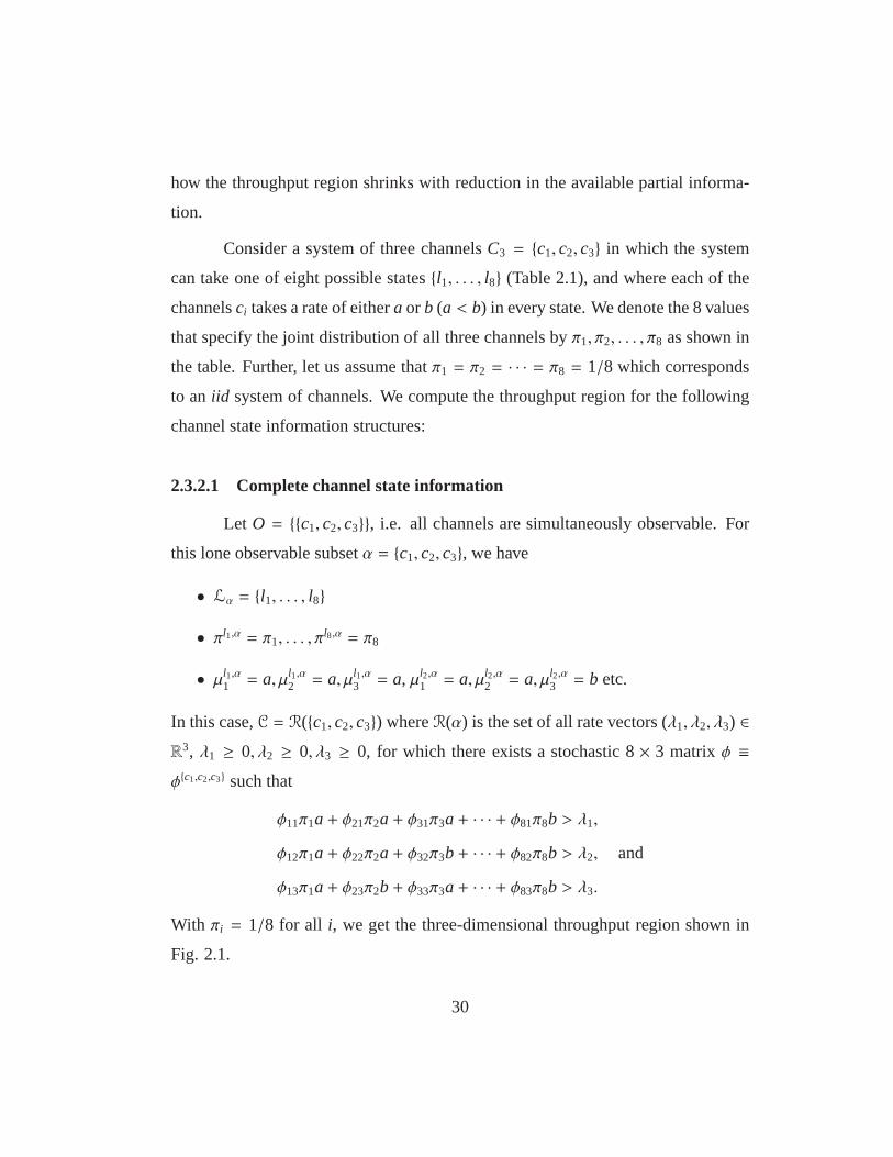
Consider a system of three channelsC3 = c1, c2, c3 in which the system

can take one of eight possible statesl1, . . . , l8 (Table 2.1), and where each of the

channelsci takes a rate of eithera or b (a < b) in every state. We denote the 8 values

that specify the joint distribution of all three channels byπ1, π2, . . . , π8 as shown in

the table. Further, let us assume thatπ1 = π2 = · · · = π8 = 1/8 which corresponds

to aniid system of channels. We compute the throughput region for thefollowing

channel state information structures:

2.3.2.1 Complete channel state information

Let O = c1, c2, c3, i.e. all channels are simultaneously observable. For

this lone observable subsetα = c1, c2, c3, we have

• Lα = l1, . . . , l8

• πl1,α = π1, . . . , πl8,α = π8

• µl1,α1 = a, µl1,α

2 = a, µl1,α3 = a, µl2,α

1 = a, µl2,α2 = a, µl2,α

3 = b etc.

In this case,C = R(c1, c2, c3) whereR(α) is the set of all rate vectors (λ1, λ2, λ3) ∈R3, λ1 ≥ 0, λ2 ≥ 0, λ3 ≥ 0, for which there exists a stochastic 8× 3 matrix φ ≡φc1,c2,c3 such that

φ11π1a+ φ21π2a+ φ31π3a+ · · · + φ81π8b > λ1,

φ12π1a+ φ22π2a+ φ32π3b+ · · · + φ82π8b > λ2, and

φ13π1a+ φ23π2b+ φ33π3a+ · · · + φ83π8b > λ3.

With πi = 1/8 for all i, we get the three-dimensional throughput region shown in

Fig. 2.1.

30

2.3.2.2 Pairwise channel state information

Let O = c1, c2, c2, c3, c3, c1, i.e. at most a pair of channels is simul-

taneously observable. Recalling the notation used in the system model, for the

observable subsetα = c1, c2 we have

• Lα = (a,a), (a,b), (b,a), (b,b)

• π(a,a),α = π1 + π2, π(a,b),α = π3 + π4, π(b,a),α = π5 + π6, π(b,b),α = π7 + π8

• µ(a,a),α1 = a, µ(a,a),α

2 = a, µ(a,b),α1 = a, µ(a,b),α

2 = b etc.

and similarly for the other observable subsetsβ = c2, c3 andγ = c3, c1. In this

case,

C = conv(R(c1, c2),R(c2, c3),R(c3, c1)).

The subset throughput regionR(c1, c2), say, is the set of all rate vectors

(λ1, λ2,0) ∈ R3, λ1 ≥ 0, λ2 ≥ 0, for which there exists a stochastic 4× 2 matrix

φ ≡ φc1,c2 such that

φ11(π1 + π2)a+ φ21(π3 + π4)a+ φ31(π5 + π6)b

+ φ41(π7 + π8)b > λ1, and

φ12(π1 + π2)a+ φ22(π3 + π4)b+ φ32(π5 + π6)a

+ φ42(π7 + π8)b > λ2.

In general, for the subsetci , cj = c1, c2, c3\ck with i, j, k ∈ 1,2,3 and

πn = 1/8 for all n, the orthogonal projection ofR(ci , cj) onto the planeλk = 0 is as

shown in Fig. 2.2. Accordingly, the throughput regionC for the system is depicted

in Fig. 2.3. Observe that:

31

• The throughput regionC is now a function only of the marginal probabilities

(π1 + π2) = P(L(t)1 = a, L(t)2 = a) etc.

• The throughput region of Fig. 2.3 has shrunk compared to the region in Fig.

2.1 due to the pairwise observability constraint.

2.3.2.3 Singleton channel state information

Let O = c1, c2, c3, i.e. only the state of one channel can be observed

in the first scheduling step. In this case,

C = conv(R(c1),R(c2),R(c3)).

Each observable subset now has only two sub-states with corresponding ratesa and

b; for instance, for the observable subsetα = c1,

• Lα = (a), (b)

• π(a),α = π1 + π2 + π3 + π4, π(b),α = π5 + π6 + π7 + π8

• µ(a),α1 = a, µ(b),α

1 = b

and similarly for the other observable subsetsβ = c2 andγ = c3. The subset

throughput regionR(c1), say, is the set of all rate vectors (λ1,0,0) ∈ R3, λ1 ≥ 0,

for which there exists a stochastic 2× 1 matrixφ = φc1 such that

φ11(π1 + π2 + π3 + π4)a+ φ21(π5 + π6 + π7 + π8)b > λ1.

Usingπn = 1/8 for all n, we get thatR(c1) is just the line segment join-

ing (0,0,0) and ((a + b)/2,0,0), and likewise forR(c2) andR(c3). Thus the

throughput regionC is the dotted simplex which is shown in Fig. 2.2. Observe that:

32

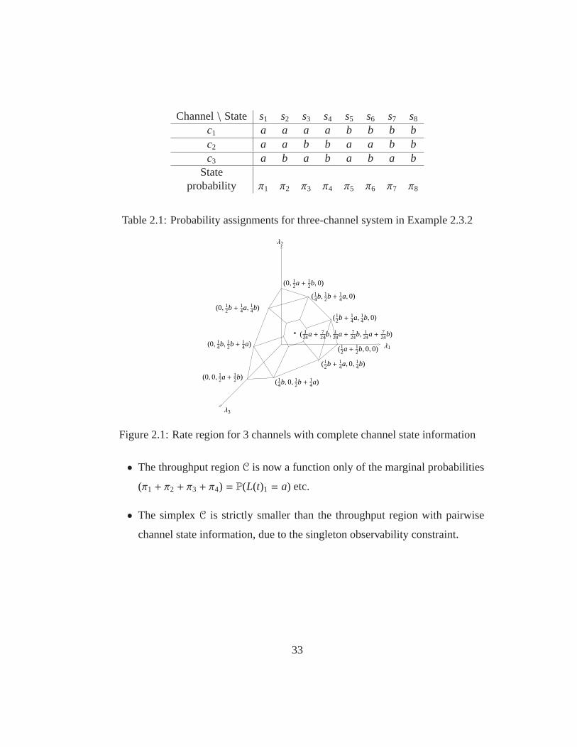
Channel\ State s1 s2 s3 s4 s5 s6 s7 s8

c1 a a a a b b b bc2 a a b b a a b bc3 a b a b a b a b

Stateprobability π1 π2 π3 π4 π5 π6 π7 π8

Table 2.1: Probability assignments for three-channel system in Example 2.3.2

( 124a+

724b,

124a+

724b,

124a+

724b)

λ1

λ3

(12b+ 1

4a, 0, 14b)

(0, 12a+ 1

2b, 0)

(14b, 1

2b+ 14a, 0)

(14b, 0, 1

2b+ 14a)

λ2

(12b+ 1

4a, 14b, 0)

(0, 14b, 1

2b+ 14a)

(12a+ 1

2b, 0, 0)

(0, 12b+ 1

4a, 14b)

(0, 0, 12a+ 1

2b)

Figure 2.1: Rate region for 3 channels with complete channel state information

• The throughput regionC is now a function only of the marginal probabilities

(π1 + π2 + π3 + π4) = P(L(t)1 = a) etc.

• The simplexC is strictly smaller than the throughput region with pairwise

channel state information, due to the singleton observability constraint.

33

λ j

λi(12a+ 1

2b, 0)

(0, 12a+ 1

2b)

(0, 0)

(14b, 1

2b+ 14a)

(12b+ 1

4a, 14b)

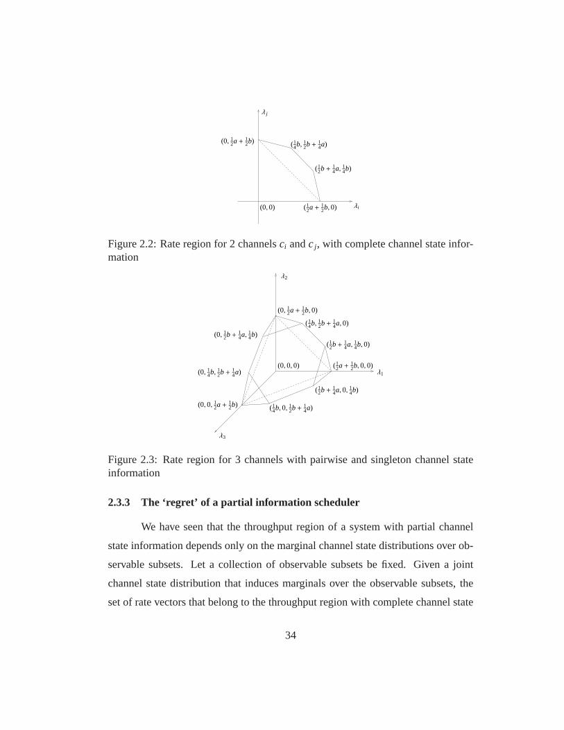
Figure 2.2: Rate region for 2 channelsci andcj, with complete channel state infor-mation

(0, 0, 0)λ1

λ2

λ3

(12a+ 1

2b, 0, 0)

(12b+ 1

4a, 14b, 0)

(12b+ 1

4a, 0, 14b)

(0, 14b, 1

2b+ 14a)

(0, 0, 12a+ 1

2b)

(0, 12a+ 1

2b, 0)

(14b, 1

2b+ 14a, 0)

(0, 12b+ 1

4a, 14b)

(14b, 0, 1

2b+ 14a)

Figure 2.3: Rate region for 3 channels with pairwise and singleton channel stateinformation

2.3.3 The ‘regret’ of a partial information scheduler

We have seen that the throughput region of a system with partial channel

state information depends only on the marginal channel state distributions over ob-

servable subsets. Let a collection of observable subsets befixed. Given a joint

channel state distribution that induces marginals over theobservable subsets, the

set of rate vectors that belong to the throughput region withcomplete channel state

34

informationexclusive ofthe throughput region with partial channel state informa-

tion is a measure of how much a partial information schedulerwhich ‘knows’ the

joint channel distribution would ‘regret’ not being able toobserve the full instanta-

neous channel state.

However, given only the marginals over observable subsets,there are, in

general, many joint distributions that are consistent withthe marginals. In this situ-

ation, a natural measure of how much a partial information scheduler would ‘regret’

not being able to observe the full instantaneous channel state is the set of rate vec-

tors that belong to the throughput region foreveryjoint distribution consistent with

the given marginals on the observable subsetsexclusive ofthe throughput region

with partial channel state information. In other words, this ‘regret region’ is the in-

tersection of the throughput regions for all systems with a consistent joint channel

state distribution, excluding the throughput region with partial channel state infor-

mation over the observable subsets. In this section, we present two examples - the

first example demonstrating that the regret region is empty and the second example

showing that the regret region can be non-empty (i.e.,anyscheduling policy with

complete channel state information canguaranteeablysupport more rates than all

policies with partial channel state information).

1. Consider the example of the previous section with pairwisechannel state in-

formation, i.e.

O = c1, c2, c2, c3, c3, c1. Suppose we know the pairwise marginals to be

as follows:P(L(t)i = µi, L(t) j = µ j) = 14, i, j ∈ 1,2,3, i , j, µi , µ j ∈ a,b.

Note that theiid joint distributionπ1 = · · · = π8 = 1/8 used earlier agrees

with these pairwise marginals.

35

These pairwise constraints give us a feasible set of possible joint channel

distributions: it is the set of vectors (π1, . . . , π8) in the simplex that satisfy the

equationsπ1 + π2 =14, π1 + π3 =

14, π1 + π4 =

14, π2 + π5 =

14, etc. In matrix

form, these constraints along with the simplex constraintsbecome

1 1 0 0 0 0 0 01 0 1 0 0 0 0 01 0 0 1 0 0 0 00 1 0 0 1 0 0 0

...

1 1 1 1 1 1 1 1

π1

π2

π3

π4

π5

π6

π7

π8

=

1/41/41/41/4...

1/41

,

with πi ≥ 0 for all i. The set of solutions for the vector~π = (π1 π2 . . . π8)T

is the set of convex combinations of the vectors~π(1) = (1/4 0 0 1/4 0 1/4 1/4 0)T

and

~π(2) = (0 1/4 1/4 0 1/4 0 0 1/4)T , i.e.,

~π ∈ Π = η~π(1) + (1− η)~π(2) : 0 ≤ η ≤ 1.

The iid joint distributionπ1 = · · · = π8 = 1/8 corresponds toη = 1/2. LetC~π

denote the throughput region with complete channel state information when

the joint distribution of channel states is~π ∈ Π. As beforeC denotes the

throughput region with pairwise partial information, as inFig. 2.3. Since

C ⊂ C~π ∀ ~π ∈ Π due to the joint distributions agreeing with the marginals,we

must have

C ⊂⋂

~π∈Π

C~π.

The hexagonal face ofC in Fig. 2.3 represents the maximum sum rate that

can be supported, and is described byλ1 + λ2 + λ3 =14a + 3

4b. We observe

36

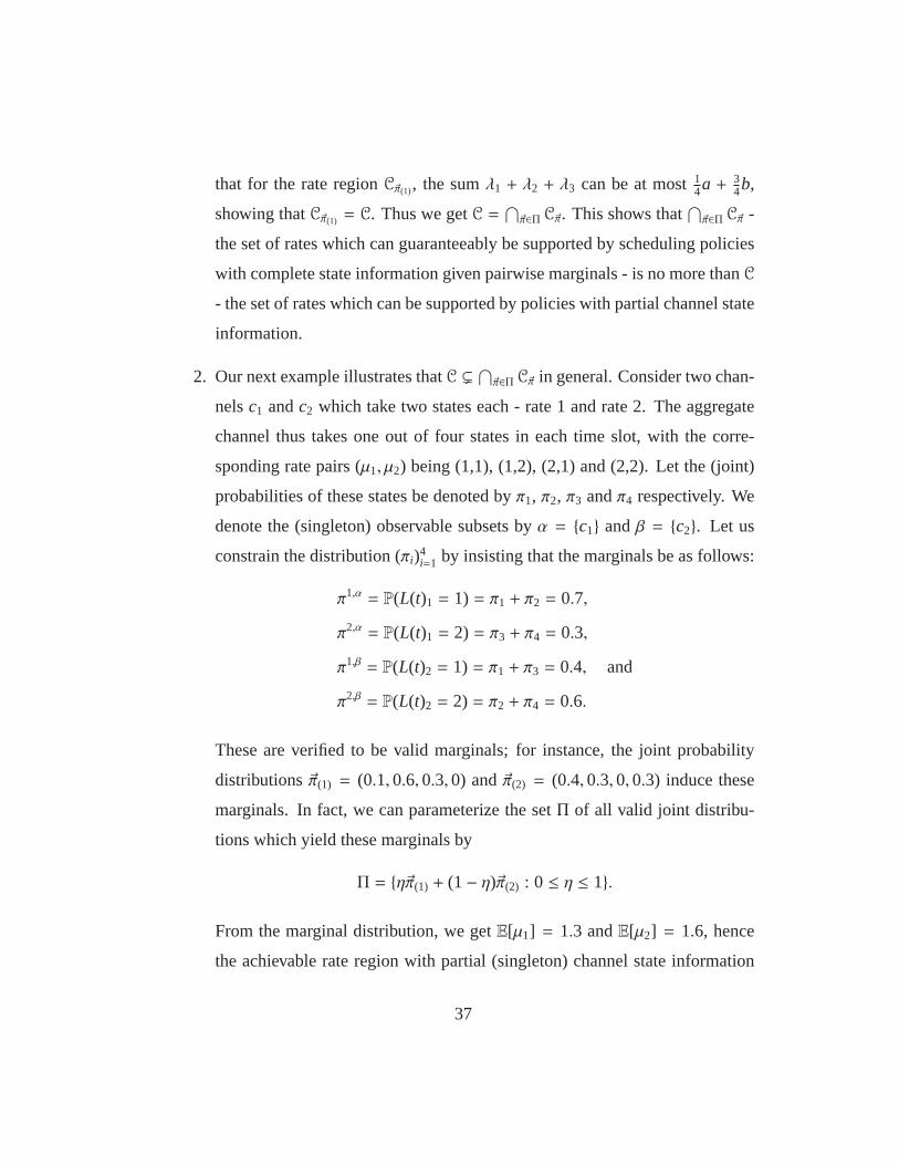
that for the rate regionC~π(1), the sumλ1 + λ2 + λ3 can be at most14a + 34b,

showing thatC~π(1) = C. Thus we getC =⋂

~π∈Π C~π. This shows that⋂

~π∈Π C~π -

the set of rates which can guaranteeably be supported by scheduling policies

with complete state information given pairwise marginals -is no more thanC

- the set of rates which can be supported by policies with partial channel state

information.

2. Our next example illustrates thatC (⋂

~π∈Π C~π in general. Consider two chan-

nelsc1 andc2 which take two states each - rate 1 and rate 2. The aggregate

channel thus takes one out of four states in each time slot, with the corre-

sponding rate pairs (µ1, µ2) being (1,1), (1,2), (2,1) and (2,2). Let the (joint)

probabilities of these states be denoted byπ1, π2, π3 andπ4 respectively. We

denote the (singleton) observable subsets byα = c1 andβ = c2. Let us

constrain the distribution (πi)4i=1 by insisting that the marginals be as follows:

π1,α = P(L(t)1 = 1) = π1 + π2 = 0.7,

π2,α = P(L(t)1 = 2) = π3 + π4 = 0.3,

π1,β = P(L(t)2 = 1) = π1 + π3 = 0.4, and

π2,β = P(L(t)2 = 2) = π2 + π4 = 0.6.

These are verified to be valid marginals; for instance, the joint probability

distributions~π(1) = (0.1,0.6,0.3,0) and~π(2) = (0.4,0.3,0,0.3) induce these

marginals. In fact, we can parameterize the setΠ of all valid joint distribu-

tions which yield these marginals by

Π = η~π(1) + (1− η)~π(2) : 0 ≤ η ≤ 1.

From the marginal distribution, we getE[µ1] = 1.3 andE[µ2] = 1.6, hence

the achievable rate region with partial (singleton) channel state information

37

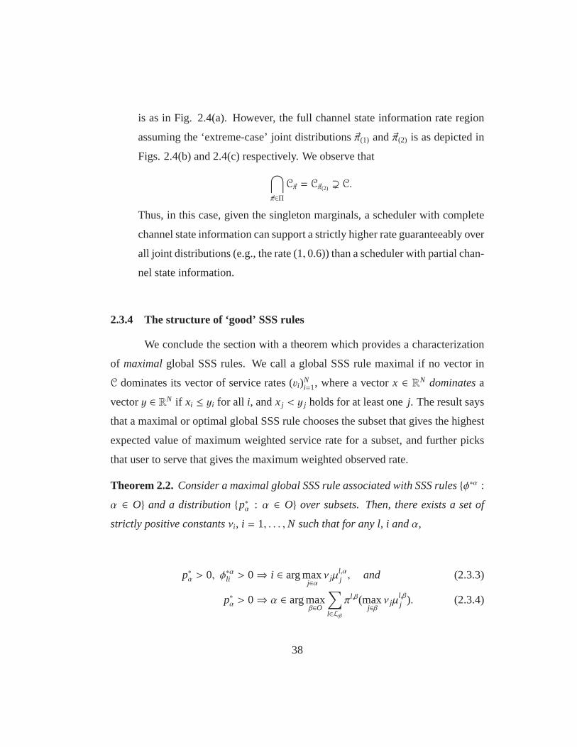
is as in Fig. 2.4(a). However, the full channel state information rate region

assuming the ‘extreme-case’ joint distributions~π(1) and~π(2) is as depicted in

Figs. 2.4(b) and 2.4(c) respectively. We observe that

⋂

~π∈Π

C~π = C~π(2) ) C.

Thus, in this case, given the singleton marginals, a scheduler with complete

channel state information can support a strictly higher rate guaranteeably over

all joint distributions (e.g., the rate (1,0.6)) than a scheduler with partial chan-

nel state information.

2.3.4 The structure of ‘good’ SSS rules

We conclude the section with a theorem which provides a characterization

of maximalglobal SSS rules. We call a global SSS rule maximal if no vector in

C dominates its vector of service rates (vi)Ni=1, where a vectorx ∈ RN dominatesa

vectory ∈ RN if xi ≤ yi for all i, andxj < y j holds for at least onej. The result says

that a maximal or optimal global SSS rule chooses the subset that gives the highest

expected value of maximum weighted service rate for a subset, and further picks

that user to serve that gives the maximum weighted observed rate.

Theorem 2.2.Consider a maximal global SSS rule associated with SSS rulesφ∗α :

α ∈ O and a distributionp∗α : α ∈ O over subsets. Then, there exists a set of

strictly positive constantsνi, i = 1, . . . ,N such that for any l, i andα,

p∗α > 0, φ∗αli > 0⇒ i ∈ arg maxj∈α

ν jµl,αj , and (2.3.3)

p∗α > 0⇒ α ∈ arg maxβ∈O

∑

l∈Lβ

πl,β(maxj∈β

ν jµl,βj ). (2.3.4)

38

(0, 1.6)

λ2

λ1(0, 0) (1.3, 0)

(a)

λ2

λ1(0, 0) (1.3, 0)

(0, 1.6) (0.6, 1.3)

(0.7, 1.2)

(1, 0.6)

(b)

(1, 0.6)

λ2

λ1(0, 0) (1.3, 0)

(0, 1.6)

(c)

Figure 2.4: (a) Rate region with singleton channel state information for 2 channels,(b) Rate region with full channel state information for jointdistributionπ(1), (c)Rate region with full channel state information for joint distributionπ(2).

According to Theorem 2.2, at timet, in the first scheduling step, a maximal

global SSS rule chooses a subsetα for which∑

l∈Lαπl,α(maxj∈α ν jµ

l,αj ) is maximized,

and further picks queuei in α which maximizesνiµl(t),αi , wherel(t) is the observed

sub-state of subsetα. We refer the reader to Appendix A.2 for the proof of Theorem

2.2.

39

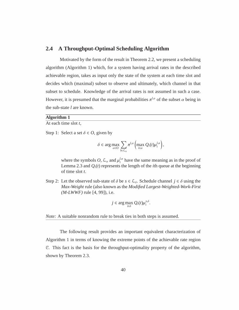
2.4 A Throughput-Optimal Scheduling Algorithm

Motivated by the form of the result in Theorem 2.2, we presenta scheduling

algorithm (Algorithm 1) which, for a system having arrival rates in the described

achievable region, takes as input only the state of the system at each time slot and

decides which (maximal) subset to observe and ultimately, which channel in that

subset to schedule. Knowledge of the arrival rates is not assumed in such a case.

However, it is presumed that the marginal probabilitiesπl,α of the subsetα being in

the sub-statel are known.

Algorithm 1At each time slott,

Step 1: Select a setδ ∈ O, given by

δ ∈ arg maxα∈O

∑

ł∈Lα

πl,α(

maxi∈α

Qi(t)µl,αi

)

,

where the symbolsO, Lα andµl,αi have the same meaning as in the proof of

Lemma 2.3 andQi(t) represents the length of theith queue at the beginningof time slott.

Step 2: Let the observed sub-state ofδ bes ∈ Lδ. Schedule channelj ∈ δ using theMax-Weightrule (also known as theModified Largest-Weighted-Work-First(M-LWWF)rule [4, 99]), i.e.

j ∈ arg maxi∈δ

Qi(t)µs,δi .

Note: A suitable nonrandom rule to break ties in both steps is assumed.

The following result provides an important equivalent characterization of

Algorithm 1 in terms of knowing the extreme points of the achievable rate region

C. This fact is the basis for the throughput-optimality property of the algorithm,

shown by Theorem 2.3.

40

Lemma 2.4. LetE be the (finite) set of extreme points for the achievable rate region

C. If subsetδ is chosen in Step 1 of Algorithm 1 at time t, then

R(δ) ∩ arg maxv∈E〈v,Q(t)〉 , ∅.

That is, the algorithm selects any subset whose rate region contains an ex-

treme point maximizing the inner product〈x,Q(t)〉 over allx ∈ E and hence a point

maximizing〈y,Q(t)〉 over ally ∈ C. Refer to Appendix A.3 for the proof of Lemma

2.4.

The chief result in this section is the following theorem, which says that the

scheduling policy defined above is throughput-optimal for scheduling with partial

channel-state information.

Theorem 2.3.Algorithm 1 makes the system stable if the vector of arrival rates lies

in the achievable region.

The proof of stability uses fluid limit machinery. Roughly, byscaling and

“compressing” time and concurrently scaling down the magnitude of the queue

length process, the discrete and random queue length process “looks like” a deter-

ministic fluid process which is driven by a (vector) constantrate fluid arrival process

(the components corresponding to the mean arrival rates to each of the users), and

whose service rate corresponds to the “average” service rate under the scheduling

algorithm. For the system we are considering, showing that such a limiting fluid

queue length trajectory has negative drift is sufficient to prove that the discrete-time

stochastic queue length process is stable (positive recurrent) [4, 58].

The full technical details are deferred to the Appendix, andhere we give

only the key Lyapunov function idea for proving negative drift. Unlike the proof

used for Theorem 3 of [4], here we face the additional difficulty of assuring that we

41

pick the correct observation subsetδ ∈ O, in addition to picking the correct queue

to serve inδ. We show that maximizing the negative drift of our Lyapunov function

is exactly the problem of maximizing the inner product〈y,Q(t)〉 over ally ∈ C. If

we pick the “wrong” subset, then maximizing the linear function above becomes

impossible. To side-step this problem, we rely on Lemma 2.4,which guarantees

that the chosen subset will indeed be one with an extreme point maximizing the

linear function.

We use the quadratic Lyapunov function

L1(y) =12

N∑

i=1

y2i (2.4.1)

for a vectory = (y1, . . . , yN). Let q(t) denote the queue-length component of a

fluid limit of the system, which in turn is an appropriate collection of almost-sure

limits of scaled system processes under uniform convergence over compact sets

(see Appendix A.4.1 for details). The following property establishes negative drift

of q(·), and (as in [4]) along with a result from [58] implies Theorem 2.3.

Lemma 2.5.Under Algorithm 1, for anyδ1 > 0, there existsδ2 > 0 such that almost

surely, at any regular point t of the fluid limit,

L1(q(t)) ≥ δ1 ⇒ ddt

L1(q(t)) ≤ −δ2 < 0.

The proof of this lemma relies on Lemma 2.4, and can be found inAppendix

A.4.1.

2.5 The Max-Sum-Queue Algorithm

The throughput-optimal scheduling algorithm in the previous section re-

quires knowledge of both the instantaneous queue lengths and marginal statistics

42

of the channel. In this section, we present a ‘simpler’ scheduling policy, called the

Max-Sum-Queue algorithm, which only uses queue-length information to pick the

subset to observe.

Algorithm 2 Max-Sum-QueueAt each time slott,

Step 1: Select a setδ ∈ O, given by

δ = arg maxα∈O

∑

i∈αQ2

i (t),

whereQi(t) denotes the length of theith queue at the beginning of time slott.

Step 2: Let the observed sub-state ofδ bes ∈ Lδ. Schedule channelj ∈ δ using theMax-Weightrule, i.e.

j = arg maxi∈δ

Qi(t)µs,δi .

Note: A suitable nonrandom rule to break ties in both steps is assumed.

We show that theMax-Sum-Queuealgorithm is throughput-optimal in two

cases of interest: (i) when the subsets inO are disjoint; and (ii) when the channel

is symmetric in the users. In the next section, we prove by example thatMax-Sum-

Queueis not throughput-optimal in general.

2.5.1 Max-Sum-Queue and disjoint subsets

The following result shows that when the collection of observable subsets

is mutually disjoint, Max-Sum-Queue is throughput-optimal.

Theorem 2.4.Under the assumption that every pair of maximal observable subsets

is disjoint, the Max-Sum-Queue scheduling algorithm makesthe system stable if the

vector of arrival rates lies in the achievable region.

43

To prove Theorem 2.4, we follow a similar route as in the previous sec-

tion, defining fluid limits and proving that a suitably definedLyapunov function has

negative drift. The Lyapunov function we use here is

L2(y) = maxβ∈O

hβ(y),

where

hβ(y) =12

∑

i∈βy2

i .

The following key lemma is used to establish the negative drift of the Lyapunov

function, and is the analog of Lemma 2.5.

Lemma 2.6. Under Max-Sum-Queue scheduling, for anyδ1 > 0, there existsδ2 > 0

such that almost surely, at any regular point t of a fluid limit,

L2(q(t)) ≥ δ1 ⇒ ddt

L2(q(t)) ≤ −δ2.

We refer the reader to Appendix A.4.2 for the details of the proof of the

lemma. There is an intuitive geometric explanation for thisresult. It is based on

two observations: first, due to the disjoint subset assumption and the Max-Sum-

Queue algorithm, if any queue is unstable, all queues are unstable; next, given an

extreme pointxα in each setR(α), the convex hull of those extreme points will

always lie on an exposed face ofC. Note that this is not true in the general case.

2.5.2 Max-Sum-Queue for symmetric channels

It is instructive to note that the reason that the presented scheduling poli-

cies work in their respective cases is that at any pointt ∈ [0,∞), they maximize

the linear objective function〈q(t),u〉 over all u in the convex polytopeC which

represents the achievable rate region. The drift of the sum-of-squares Lyapunov

44

function defined by (2.4.1) happens to be precisely the difference between〈q(t), λ〉and maxu∈C〈q(t),u〉. This geometric interpretation allows us to prove the useful re-

sult that Max-Sum-Queue is actually throughput-optimal for systems ofsymmetric

channels and subsets. A symmetric system is where the distribution of the aggre-

gate channel stateL(t) is such thatevery permutation of a given aggregate channel

state occurs with the same probability. For instance, for a system of three channels

c1, c2, c3, the aggregate channel state distributed as (1,0,0), (0,1,0) and (0,0,1)

equally likelyqualifiesas a symmetric system, whereas the system with the aggre-

gate channel state distributed as (1,0,0), (0,1,0), (0,0,1) and (0,0,0) equally likely

does not qualifyas a symmetric system.

Theorem 2.5.Consider a symmetric system, i.e., where the observable subsets are

all the subsets of a fixed cardinality K. For such a system, Max-Sum-Queue is

throughput-optimal.

Proof. Let λ be the vector of arrival rates to the system ofN channels represented

by S = 1, . . . ,N, such thatλ ∈ intC. As before, we consider the drift of the

sum-of-squares Lyapunov function defined by (2.4.1):

ddt

L1(q(t)) =N∑

i=1

qi(t)(λi − fi(t))

= 〈q(t), λ〉 − 〈q(t), f (t)〉,

where f (t) ≡ ( fi(t))Ni=1 is the instantaneous vector of service rates chosen by Max-

Sum-Queue at timet in the fluid time scale. We show thatf (t) ∈ C maximizes the

inner product〈q(t), x〉 over all x ∈ C or equivalently over all the extreme points of

C; this establishes that the drift ofL1(q(t)) is strictly negative and bounded away

from zero and hence Max-Sum-Queue is throughput-optimal.

45

The subsets which Max-Sum-Queue picks for scheduling att are the ones

that contain the topK queues in the system. Without loss of generality, letq1(t) ≥q2(t) ≥ . . . ≥ qN(t), and let

A = arg maxβ⊂S,|β|=K

∑

i∈βq2

i (t).

Every setα ∈ A is picked by Max-Sum-Queue in the fluid timescale, and

thus has the same queue values ordered in descending order. Further, since the

channels are symmetric, every subset rate regionR(β) for β ⊂ S, |β| = K, is identical

up to a permutation of indices. It follows that the extreme points of C maximizing

〈·,q(t)〉 must lie in the rate regionsR(α) whereα ∈ A, since only theK heaviest

queues can maximize this inner product over all permutations of extreme points.

Since these extreme points are precisely the ones picked by Max-Sum-

Queue in each subset, and thatf (t) lies in the convex hull of these extreme points,

f (t) maximizes the inner product〈q(t), x〉 over allx ∈ C, and we are done.

For an alternative view of why the Max-Sum-Queue policy works for sym-

metric channels, refer to Appendix A.5.

2.6 Max-Sum-Queue applied to arbitrary subsets

In this section we show that the simpleMax-Sum-Queuescheduling algo-

rithm is not throughput-optimal in general. An intuitive fluid argument is presented

first, followed by a formal proof.

Consider a system of three channelsc1, c2 andc3. The system assumes four

possible statesS1, S2, S3 andS4 with the corresponding channel rates, expressed

by (rate ofc1, rate ofc2, rate ofc3), being (100,100,2), (100,200,2), (200,100,2)

46

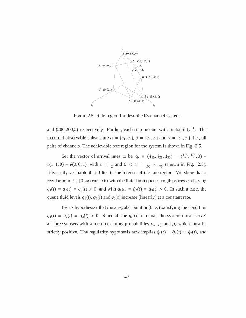
λa

λ1λ3

C : (50, 125, 0)

E : (150, 0, 0)

B : (0, 150, 0)

A : (0, 100, 1)

G : (0, 0, 2)

F : (100, 0, 1)

D : (125, 50, 0)

λ2

λb

Figure 2.5: Rate region for described 3-channel system

and (200,200,2) respectively. Further, each state occurs with probability 14. The

maximal observable subsets areα = c1, c2, β = c2, c3 andγ = c3, c1, i.e., all

pairs of channels. The achievable rate region for the systemis shown in Fig. 2.5.

Set the vector of arrival rates to beλb ≡ (λ1b, λ2b, λ3b) = (1752 ,

1752 ,0) −

ǫ(1,1,0) + δ(0,0,1), with ǫ = 12 and 0 < δ = 1

100 < 175 (shown in Fig. 2.5).

It is easily verifiable thatλ lies in the interior of the rate region. We show that a

regular pointt ∈ [0,∞) can exist with the fluid-limit queue-length process satisfying

q1(t) = q2(t) = q3(t) > 0, and withq1(t) = q2(t) = q3(t) > 0. In such a case, the

queue fluid levelsq1(t), q2(t) andq3(t) increase (linearly) at a constant rate.

Let us hypothesize thatt is a regular point in [0,∞) satisfying the condition

q1(t) = q2(t) = q3(t) > 0. Since all theqi(t) are equal, the system must ‘serve’

all three subsets with some timesharing probabilitiespα, pβ andpγ which must be

strictly positive. The regularity hypothesis now implies ˙q1(t) = q2(t) = q3(t), and

47

hence

⇒ λ1b − 150pγ −1752

pα

= λ2b − 150pβ −1752

pα

= λ3b − 0 = δ

⇒ pγ = pβ, and

150pβ +1752

pα = λ2b − δ = 86.99.

Together withpα+ pβ+ pγ = 1, we getpβ = pγ ≈ 0.02 andpα ≈ 0.96 which

is the unique timesharing solution between the subsetsα, β andγ. Hencet is indeed

a regular point, all the queue fluid limits are equal, and increase linearly at the same

rateδ > 0.

Remarks:

1. We observe that the (mutually exclusive) conditionsq1(t) = q2(t) > q3(t) and

q1(t) = q2(t) < q3(t) lead to all theqi becoming equal within finite time.

Hence the stateq1(t) = q2(t) = q3(t) is an ‘unstable attractor’ for the fluid

limits in this sense.

2. For the arrival rate vectorλa = (87,87,0) (shown in Fig. 2.5), we can sim-

ilarly show that starting fromq1(0) = q2(0) = q3(0) = c > 0 implies that

q1(t) = q2(t) = q3(t) = c at all timest ∈ [0,∞).

Next, as a consequence of the linear growth, we show that the Markov chain

describing the state of the system is transient, which implies that all the queues grow

without bound almost surely. This is accomplished by demonstrating two crucial

properties -

48

• With high probability the aggregate state of the system of channels is dis-

tributed according to the invariant distributionπ of the Markov chain describ-

ing its evolution, and

• Whenever the channel states are typically distributed thus,the smallest queue

always grows with a rate bounded away from zero.

Theorem 2.6. The three-channel system considered is unstable under the Max-

Sum-Queue scheduling policy. Furthermore, the Markov chain describing the evo-

lution of its state is transient.

The proof is deferred to Appendix A.6.

2.7 Conclusions and Future Work

The Max-Weightrule is a striking example of a simple feedback based

scheduling policy that is throughput-optimal. Likewise, with partial channel state

information, the algorithm we presented which uses queue lengths and expected

channel states is throughput-optimal. Under constraints like disjoint set observa-

tions or symmetric channels, just looking at the heaviest queues suffices for stabil-

ity. Both the scheduling algorithms we studied for the partial information case can

be viewed as extensions of Max-Weight, which inherit its property of throughput-

optimality.

Chapter 3 continues studying scheduling with subset-based partial informa-

tion by analyzing queue length and buffer overflow performance for the downlink

system modeled here. It develops a complete framework in which decay rates of

queue length tails can be studied. Other possible directions for future work in-

clude extensions to network-wide scheduling with partial observability of channels.

49

Can the presented scheduling policies be extended to network-wide policies as with

Max-Weightand the Back Pressure algorithm [100]?

Another line of research would be to study what happens when the channel

is correlated across time and when the scheduler is allowed to use the whole past

history to make service decisions. For instance, allowing the channel to be Marko-

vian in time leads to a Partially Observable Markov DecisionProcess (POMDP)

problem, and it is interesting to investigate the stabilityregion and the existence of

throughput-optimal scheduling policies. Is scheduling based on queue lengths and

expected channel states still optimal?

50

Chapter 3

Downlink Scheduling: Buffer Overflow Performance

3.1 Introduction

Next-generation wireless cellular systems such as LTE-Advanced [68] and

WiMAX [3] promise high-speed packet-switched data services for a variety of ap-

plications, including file transfer, peer-to-peer sharingand real-time audio/video

streaming. Together with maximizing data rates or throughput, the scheduling al-

gorithm at the cellular base station must keep packet delaysin the system low, in

order to support highly delay-sensitive applications likereal-time video streaming.

There has been much recent work to develop wireless scheduling algorithms

with optimal throughput and/or delay performance [4, 75, 90, 98, 102]. Such op-

portunistic scheduling algorithms utilize instantaneouswireless Channel State In-

formation (CSI) from all users to make good scheduling decisions. However, as we

have seen earlier, in a practical situation with a large number of users in the net-

work, channel state feedback resources could potentially be limited, i.e., it might

be infeasible to acquire complete instantaneous CSI from allchannels due to band-

width and latency limitations. Instead, it might be possible to request CSI feedback

from only a subset of users at each time. Thus, it is importantto develop algorithms

that can schedule using only partial CSI rather than completeCSI, and at the same

time afford the best possible delay performance.

Using partial CSI from subsets of channels entails a new dimension of op-

portunism in wireless scheduling. The scheduling algorithm needs to make a careful

51

choice of which subsets to sample, together with how to use the sampled CSI for

scheduling. We saw in Chapter 2 that certain extensions of complete-CSI schedul-

ing algorithms to the partial-CSI setting have throughput-optimal properties, yet it

is not clear how they perform in the sense of packet delays. The general structure

of low-delay, partial-CSI scheduling algorithms remains unknown, i.e., how an al-

gorithm should choose “good” subsets of channels, whether any additional backlog

or statistical information is needed for picking subsets, and if so, how much, how

users should be scheduled in the observed subset etc.

Throughput-maximizing scheduling has been studied with different forms

of partial CSI, including infrequent channel state measurements [48], group/random-

access based quantized channel state feedback [69, 97], optimal channel state prob-

ing with costs [13, 15], delayed CSI [108] and subset-based CSI[37]. However,

to date, neither the structure nor performance results for queue overflow tails under

scheduling with partial CSI are known.

In this chapter, we develop algorithms for wireless scheduling that use only

partial CSI from subsets of channels, and that also enjoy highqueue overflow per-

formance guarantees. We consider a wireless downlink wherea base station sched-

ules users using partial CSI from subsets of channels. Viewing the system queue

lengths as a surrogate for packet delays, we seek schedulingstrategies that can keep

the longest queue in the system as short as possible, i.e., minimize the likelihood

of overflow of the longest queue. We describe a new schedulingalgorithm, that we

termMax-Exp, that obtains partial CSI relying on just current queue lengths and no

other auxiliary information. Employing sample-path largedeviations techniques,

we show that when the observable channel subsets are disjoint, Max-Exp yields

the best decay rate for the longest-queue overflow probability, across all scheduling

strategies which use subset-based CSI to schedule users. To the best of our knowl-

52

edge, this is the first work that analyzes queue-overflow performance for scheduling

with the information structure of partial CSI, and that provides a simple scheduling

algorithm needing no extra statistical information which is actually rate-function

optimal for buffer overflow.

From a technical standpoint, sample-path large deviationstechniques have

successfully been used to analyze wireless scheduling algorithms [8, 75, 90, 102];

yet, significant new analytical challenges emerge when studying the large devia-

tions behavior of scheduling strategies that cannot accessthe full state of the system.

A chief difference in this regard arises from the fact that when scheduling is carried

out by observing thecompletestate/randomness of the system, large deviations oc-

cur depending on how the scheduler responds to atypical channel state behavior. In

other words, a natural cause-effect relationship between the channel state process

and scheduling actions is the basis for the analysis of largedeviations performance.

On the other hand, whenpartial channel state isacquiredselectively by a schedul-

ing algorithm, this cause-effect sequence is reversed – it is the algorithm that first

decides what part of the channel state to sample; subsequently, this dynamic por-

tion of the channel state can respond by behaving atypically. Viewed differently, the

scheduling information structure no longer falls into an “experts” setting (all chan-

nel rates known in advance), but rather into a “bandit” setting (only chosen channel

rates known), implying a fundamental change in the large deviations dynamics. In-

deed, we are able to show that the this difference results in a significantly different

rate function than that encountered in the former complete-CSI case.

Also, the standard approach of analyzing queue overflow probability ex-

ponents using continuity of queue-length/delays as functions of the arrivals and

channel processes [81, 107] becomes cumbersome due to the complex two-stage

sampling and scheduling structure of scheduling with partial CSI. Thus, we are

53

led to develop new sample-path large deviations results forprocesses with dynami-

cally (and predictably) sampled randomness, which help to bound the resulting rate

functions via connections to appropriate variational problems. We believe that these

techniques and results are of independent interest as toolsto analyze the behavior

of scheduling policies that can only sample parts of the system state.

3.1.1 Summary of Contributions

In this chapter, we describe a new scheduling algorithm – Max-Exp – for

wireless scheduling with Channel State Information (CSI) restricted to a collection

of observable channel subsets. The Max-Exp algorithm picks a subset of channels

to acquire CSI depending on an appropriate exponentiated sumof the subset queue

lengths. Having done that, it uses the well-known Exponential rule [85] to sched-

ule a user from the subset using the obtained CSI. Thus,Max-Exp does not need

any additional information (e.g. traffic/channel statistics) other than queue lengths

to dynamically pick subsets, and only the instantaneous subset channel states to

schedule users. We then show the following:

1. We derive a lower bound on the rate function for overflow of the longest

queue under the Max-Exp scheduling algorithm, using sample-path large de-

viations tools and their connection to variational optimal-control problems. A

key technical contribution here is developing large deviations properties for

processes obtained by predictably sampling independent and identically dis-

tributed (iid) sequences. These results are used to show that the sample-path

large deviations rate function, for algorithms that sampleonly portions of the

channel state, not only depends on the standard Cramer empirical rate func-

tions of the sampled portions [23], but also relies crucially on thesampling

frequenciesof the portions.

54

Conversely, we also show universal upper bounds on the queue overflow rate

function of any scheduling policy that accesses partial, subset-based CSI.

For this purpose, we develop a novel martingale-based argument that, to-

gether with exponentially-twisted channel distributions, yields a universal

upper bound on the buffer overflow probability exponent.

2. In the case where the collection of observable subsets available to the sched-

uler is disjoint, we prove that the lower bound on the large deviations buffer

overflow rate function for Max-Exp matches the uniform upperbound on the

rate function over all algorithms. This not only characterizes the exact buffer

overflow exponent of the Max-Exp algorithm, but also shows rather surpris-

ingly that the simple Max-Exp strategy yields the optimal overflow exponent

across all scheduling rules using partial CSI. As a side consequence, this

shows that for scheduling with singleton subsets of users, merely scheduling

the user with the longest queue at each time slot – a greedy strategy when no

CSI is available beforehand – is large-deviations rate function-optimal.

3.2 System Model

This chapter uses the same wireless system model introducedin Chapter 2.

For clarity of presentation, we describe the essential features of the model here.

We consider a standard model of a wireless downlink system [4]: a time-

slotted system ofN users serviced by a single base station or server acrossN com-

munication channels. In each time slotk ∈ 0,1,2, . . ., the dynamics of the system

are governed by three primary components:

1. Arrivals: An integer number of data packetsAi(k) arrives to useri, i =

55

1, . . . ,N. Packets get queued at their respective users if they are notimmedi-

ately transmitted.

2. Channel states:The set ofN channels assumes a randomchannel state R(k),

i.e. anN-tuple of integerinstantaneous service rates(r1, . . . , rN). At time slot

k, let the instantaneous service rates be (R1(k), . . . ,RN(k)).

3. Scheduling:One userU(k) ∈ 1, . . . ,N is picked by a scheduling algorithm

for service, and a number of packets not exceeding its instantaneous service

rate is removed from its queue. LetDi(k) denote whether useri is scheduled

in time slotk (Di(k) = 1), or not (Di(k) = 0). Then, useri’s queue length

(denoted byQi(·)) evolves asQi(k+ 1) = [Qi(k)+Ai(k)−Di(k)Ri(k)]+, where

x+ ≡ max(x,0).

We assume the following about the stochastic dynamics of thearrival and channel

state processes:

Assumption 1 (Arrivals): Each useri’s arrival process (Ai(k))∞t=0 is deterministic

and equal toλi at all time slots. This is done merely for notational simplicity, and it

is straightforward to relax this assumption to bounded iid arrival processes.

Assumption 2 (Channel States):The joint channel statesR(k), k = 0,1,2, . . . are

independent and identically distributed across time, and take values from a finite set

R of integerN-tuples. Note that the channel states can haveany joint distribution

and can thus be correlatedacross channels/users.

Scheduling Model: Under scheduling withpartial channel state information, at

each time slotk, the scheduling algorithm makestwosequential choices to schedule

a user:

• Step 1:Pick asubset S(k) of the N channels, from a given collectionO of

56

observable subsets. This choice can depend on all random variables in time

slots up to and includingk except the channel stateR(k).

• Step 2:Once the subsetS(k) of channels is chosen, the instantaneous service

rates (Ri(k))i∈S(k) are revealed/available to the scheduling algorithm, and it

chooses a userU(k) ∈ S(k) for service, possibly depending on these service

rates.

Note that at each time, the channel state information available to the scheduling

algorithm is restricted to the chosen subsetS(k) of channels, as opposed to the full

CSI case where all the service rates (Ri(k))Ni=1 are available. For further detailed

discussion about this scheduling model, we refer the readerto Section 2.2.

3.3 Objective, Algorithms and Main Results

Our focus in this chapter is to design scheduling algorithmsthat reduce

the likelihood of large queues in the system. Specifically, we seek to minimize

the stationary probability (when it exists) that the longest queue in the system

||Q(k)||∞= maxi Qi(k) exceeds a thresholdn. Alternatively, our goal is to maxi-

mize theexponentor decay rateof the exceedance probability

I= − lim

n→∞

1n

logP [||Q(k)||∞ ≥ n]

(when the limit exists), for scheduling algorithms thatobserve only partial channel

statewhile scheduling. The usefulness of this exponent stems from the approxima-

tion

P[||Q(k)||∞ ≥ n] ≈ e−nI (largen)

that it affords for the actual overflow probabilities. Also, as observed in [102], for

the case of deterministic arrivals, the tail of the probability distribution for the delay

57

Di(k) until transmission experienced by a packet for useri arriving at time slotk is

directly related to that of its queue length by

P[Di(k) ≥ di] = P[Qi(k) ≥ λi(di − 1)].

Hence, valuable insights can be gained about the exponents of packet delays from

those of the system queue lengths.

With this performance objective in mind, we introduce a new scheduling

algorithmMax-Expspecified as follows:

Algorithm 3 Max-ExpAt each time slotk, breaking ties arbitrarily,

Step 1: Choose a subsetS(k), from the collectionO of observable subsets, suchthat

∑

i∈S(k)

exp

Qi(k)

1+√

Q(k)

is maximized (hereQ(k)= 1

N

∑Ni=1 Qi(k)).

Step 2: Schedule a useri ∈ S(k) such thatRi(k) exp

(

Qi (k)

1+√

Q(k)

)

is maximized (the

Exponential rule [85]).

By our probabilistic assumptions on the channel state process, Max-Exp

makes the vector process of queue lengths at each time a discrete-time Markov

chain. Following standard convention [4, 27, 64], we term the set of arrival rates

λ ≡ (λi)Ni=1 for which this Markov chain is positive-recurrent as thethroughput

regionof Max-Exp. In order not to deviate from the main focus of the chapter, we

state without proof that the throughput region of Max-Exp contains that of any other

scheduling algorithm, i.e., Max-Exp isthroughput-optimal. Our main result states

58

that Max-Exp yields the best (exponential) rate of decay of the tail of the longest

queue over all strategies that use partial CSI from disjoint subsets:

Theorem 3.1 (Large Deviations Optimality of Max-Exp for general disjoint ob-

servable subsets). The following holds when the system’s arrival ratesλ lie in the

interior of the throughput region of the Max-Exp schedulingalgorithm:

1. LetP denote the stationary probability distribution that the Max-Exp algo-

rithm induces on the vector of queue lengths. Then, there exists J∗ > 0 such

that

− lim supn→∞

1n

logP [||Q(0)||∞ ≥ n] ≥ J∗.

2. Letπ be an arbitrary scheduling rule that induces a stationary distribution

Pπ on the vector of queue lengths. If the system of observable subsetsO is

disjoint, then

− lim infn→∞

1n

logPπ [||Q(0)||∞ ≥ n] ≤ J∗.

Thus, Max-Exp has the optimal large-deviations exponent (equal to J∗) over

all stabilizing scheduling policies with subset-based partial channel state in-

formation.

Theorem 3.1 highlights the striking property that Max-Exp,using only cur-

rent queue length information to sample channel subsets andthe Exponential rule

to schedule a sampled channel, yields thefastest decayof the buffer overflow prob-

ability across the whole spectrum of partial-CSI schedulingalgorithms – including

those that potentially use additional statistical information, traffic characteristics

etc. The crucial scheduling step in Max-Exp is Step 1, which essentially sam-

ples the “right” channel subset depending on queue lengths.The result shows that

queue length feedback is sufficient to guarantee good delay performance, provided

59

suitable subsets of channel states are sampled as with the Max-Exp scheduling al-

gorithm. We remark that the optimality of Max-Exp continuesto hold even when

all queue lengths are delayed by any bounded amount.

En route to proving Theorem 3.1, we develop lower bounds for the large

deviations exponents of partially and deterministically sampled iid processes, that

are of independent interest. This results in a new rate function formulation in terms

of variational optimization, that differs significantly from existing rate functions

[75, 81, 90, 101, 102, 107] by explicitly incorporating partial channel state sam-

pling behavior. Standard optimal control approaches for the full-CSI case cannot

be applied to analyze partial-CSI scheduling algorithms – since only a portion of

the channel state is revealed to the scheduler, the channel state process can cause

large deviations by behaving atypically just in the revealed portion, and not jointly

as a whole.

A related challenge arises in the process of finding universal upper bounds

on the decay rate for arbitrary partial-CSI scheduling policies. Recent large-deviations

work in full-CSI scheduling [90, 102] accomplishes this by calculating the “cost” of

universal channel-state sample paths that cause buffer overflow under any schedul-

ing algorithm; however, this procedure fails for algorithms actively sampling the

channel state, since the cost of such sample paths intimately depends on the sub-

set sampling behavior. To overcome this, we use a martingale-based argument in

a novel way with the standard exponential tilting method to prove universal upper

bounds on the exponent.

Observe that Max-Exp reduces to the following Max-Queue scheduling al-

gorithm when the observable subsets are all the singleton users:

Thus, an immediate corollary of Theorem 3.1 is the followingoptimality

result for Max-Queue when the observable user subsets are restricted to singletons,

60

Algorithm 4 Max-QueueAt each time slotk, breaking ties arbitrarily,

Steps 1, 2: Schedule a useri such thatQi(k) is maximized.

i.e., when there is effectively no CSI to use in scheduling:

Corollary 3.1 (Large Deviations Optimality of Max-Queue for singleton observ-

able subsets). If the system’s arrival ratesλ lie in the interior of the throughput

region of the Max-Queue scheduling algorithm, then Max-Queue has the optimal

large-deviations exponent of the queue overflow probability over all stabilizing

scheduling policies that can sample only individual channel states.

Road map to Theorem 3.1:Though Theorem 3.1 for Max-Exp is our chief

result, we prove it by first establishing the optimality result for Max-Queue (Corol-

lary 3.1), and then extending the argument to the setting of general disjoint subsets.

This is mainly because the essence of the optimality lies in the key subset selection

step, and restricting attention to the case of singleton observable subsets allows us

to concentrate on how subset selection influences the large deviations rate function

of buffer overflow. Technically, another reason for this order of working is that

Max-Queue can naturally be analyzed with the standardO(n) fluid scaling, whereas

showing the optimality property for Max-Exp requires usinga more complex fluid

limit framework at theO(√

n) “local” fluid time-scale [85, 90].

3.4 Sample Path Large Deviations Framework

This section lays down preliminaries for the sample-path large deviations

techniques we use to study overflow probabilities of wireless scheduling algorithms.

61

Much of this framework is standard in recent large-deviations analyses of wireless

systems [75, 90, 102], but we include it for completeness.

Fix an integerT > 0, and consider a sequence of (independent) queue-

ing systems indexed byn = 1,2, . . ., each with its own arrival and channel state

processes, and evolving as described in Section 3.2. Henceforth, we explicitly ref-

erence by the superscript (n) any quantity associated with thenth system. For any

(possibly vector-valued) random processX(n)(k), k = 0,1,2, . . . in thenth system,

let us define its scaled (by 1/n), shifted and piecewise linear versionx(n)(·) on the

interval [−T,0] as follows:

x(n)(t) =

X(n)(n(t+T))n , n(t + T) an integer;

X(n)(⌊n(t+T)⌋)n +

X(n)(⌈n(t+T)⌉)−X(n)(⌊n(t+T)⌋)n(n(t+T)−⌊n(t+T)⌋) , otherwise.

In other words, we transform the discrete-time processX(n)(·) on 0,1,2, . . . ,nT

to the piecewise linear and continuous processx(n)(·) on [−T,0] by compressing

time by a factor ofn, shifting time byT, scaling space by1n and finally linearly

interpolating between the discrete points.

For thenth queueing system, withk a nonnegative integer, letF(n)i (k) be the

total number of packets to queuei that arrived by time slotk, and F(n)i (k) be the

number of packets that were served from queuei by time slotk. For a subsetα of

channels, letC(n)α (k) denote the total number of time slots beforek when subsetα

was chosen by the scheduling algorithm. We also define itssub-state R(n)α (k) to be

the vector of instantaneous service ratesR(n)(k) restricted to the coordinates ofα,

i.e., R(n)α (k) = (R(n)

i (k))i∈α. Denote byGα,(n)r (k) the total number of time slots before

time slotk when the subsetαwas picked and its sub-state wasr; and byGα,(n)ri (k) the

number of time slots before timek when subsetαwas picked, its observed sub-state

wasr and queuei ∈ α was ultimately scheduled for service. As stated earlier, we

62

denote byQ(n)i (k) the length of queuei at time slotk, whose evolution is specified

in Section 3.2. Finally, we letM(n)(k) denote the vector-valued partial sums process

corresponding to the sampled ratesR(n)(k)δS(k), i.e.,M(n)(k)=

∑ki=0 R(n)(i)δS(i).

Our assumptions on deterministic arrivals and a finite support for the chan-

nel state vectorR(k) in each time slotk imply that the scaled processesf (n)i (·),

f (n)i (·), c(n)

α (·), gα,(n)r (·), gα,(n)

ri (·), q(n)i (·) andm(n)(·), on the interval [−T,0], are uni-

formly Lipschitz-continuous (with Lipschitz constantL, say) for all n. By the

Arzela-Ascoli theorem, asn→ ∞, Suppose a sequence of scaled processesf (n)i (·),

f (n)i (·), c(n)

α (·), gα,(n)r (·), gα,(n)

ri (·), q(n)i (·) andm(n)(·) converges uniformly (over [−T,0])

to the corresponding “limit functions”fi(·), fi(·), cα(·), gαr (·), gαri (·), qi(·) andm(·) on

[−T,0]. We call any such collection of joint limit functions, obtained via appropri-

ately scaled pre-limit sample paths, aFluid Sample Path (FSP)(we use the super-

scriptT to emphasize the finite horizon [−T,0] if desired). We note that fluid sam-

ple paths inherit Lipschitz continuity (with the same Lipschitz constant) from their

corresponding pre-limit processes indexed byn (when the pre-limits are Lipschitz-

continuous), and are thus differentiable almost everywhere.

3.5 Analysis: Singleton Subsets and the Max-Queue Algorithm

In this section, we treat the simpler setting where the disjoint observable

subsets are all the singleton users in the system, i.e.,O = i : 1 ≤ i ≤ N. We

use the subscripti to refer to subsetsα. Thus, scheduling algorithms are essentially

sampling algorithms – Step 2 of the algorithm is to schedule the lone user whose

channel state is observed. The following three key steps areinvolved in showing

that Max-Queue yields the optimal decay rate of buffer overflow probability:

1. Lower-bounding Max-Queue’s Decay Rate: Large Deviations for Sam-

63

pled ProcessesShowing a lower bound on the overflow exponent of Max-

Queue for a finite horizon starting from empty queues, using sample path

large deviations for sampled processes and connections to associated vari-

ational problems, and extending the finite-horizon result to a lower bound

over an “infinite horizon”, i.e., on the stationary queue overflow probabil-

ity for Max-Queue, using standard techniques fromFriedlin-Wentzell theory

[90, 102],

2. Universal Large Deviations Upper Bounds for all policiesProvide a way

of upper-bounding the queue overflow exponent uniformly foranyscheduling

policy overflow exponent by “twisting” the subset marginal channel state dis-

tributions, constructing “straight-line” overflow eventsand estimating their

probabilities,

3. Large Deviations Optimality of the Max-Queue Policy: Connecting the

Upper and Lower BoundsShow that the lower bound on the rate function

for the stationary queue overflow probability for Max-Queueactually acts as

a uniform upper bound on the rate function for overflow foranyscheduling

algorithm

3.5.1 Lower-bounding Max-Queue’s Decay Rate: Large Deviations for Sam-pled Processes

Consider the queueing system operating under an arbitrarynonrandomschedul-

ing algorithm, i.e., the algorithm’s choice of a singleton user in the current time slot

is a deterministic function of the entire history of observed users’ indices and chan-

nel states, and does not depend on the unobserved channel states in the past. Max-

Queue with deterministic tie-breaking (e.g., pick the lowest-indexed queue when

there are two or more longest queues) is an example of a nonrandom scheduling

64

algorithm, since the current user chosen depends on accumulated queue lengths,

which in turn depend directly on the channel rates obtained as a result of past

scheduling choices.

The sequence of observed users and their channel states under a nonrandom

scheduling algorithm is an outcome of sampling an iid vector-valued process (i.e.,

the full channel state) in a nonrandom andpredictable(i.e., with sampling indices

depending only on past observed history) manner. Our first key result (Proposition

3.1) essentially furnishes a lower bound for the deviation probability of the queue-

length process (equivalently the cumulative process of observed channel states) in

time slots 0, . . . ,nT, in terms of a novel sample-path large deviations rate function

of the user selection and channel state paths.

Let us fix T > 0. For q0 ∈ RN, let Pn,Tq0 be the probability measure of

then-th queueing system conditioned on starting the system atQ(n)(0) = nq0 (i.e.

q(n)(−T) = q0). If we denote byC+L

([−T,0]) the space of nonnegativeRN-valued

Lipschitz functions on [−T,0] equipped with the supremum norm, then we have:

Proposition 3.1 (Large Deviations for Sampled Processes). Let Q be a closed set

in RN, and letΓ be a closed set of trajectories inC+L

([−T,0]). Then, under any

deterministic scheduling policy,

− lim supn→∞

1n

log supq0∈QP

n,Tq0

[

q(n) ∈ Γ]

≥ inf(mT ,cT ,qT )

∫ 0

−T

N∑

i=1

ci(t)Λ∗i

(

mi(t)ci(t)

)

dt (3.5.1)

subject to (mT , cT ,qT) an FSP,

qT(−T) ∈ Q,qT ∈ Γ,

with Λ∗i (·) being the Legendre-Fenchel dual ofΛi(λ) = logE[eλRi (0)] (the Cramer

rate function for the empirical mean of the marginal rate(Ri(k))k).

65

Proposition 3.1 states that the “correct” sample-path large deviations rate

function, for algorithms that can sample only singleton subsets of channels, is a

combination of the standard rate functionsΛ∗i for the empirical means of individual

channel ratesweighted by the corresponding channel selection frequencies ci. Note

the crucial dependence of the rate function on the subset selection process, captured

by weightingΛ∗i by ci in (3.5.1) – a significant departure from the rate function

studied for the standard case of full channel state information where there is no

pre-weighting by the algorithm-dependent factor ˙c [90, 102].

The proof of this result relies on the key fact that the sample-path trajectory

of any nonrandom scheduling/sampling algorithm is completely determined by only

thesampleduser’s index and the observed channel state at all times, instead of the

entire joint channel state process with unobserved channelstates. Also, since only

one component of the joint channel state is used at each instant, there is no loss

of generality in assuming that all the channel state processes are independent with

the original marginals. These two properties, together with exchangeability of the

channel state process, allow us to derive a large deviationsrate function for the

random process of sampled channel states, which is further transformed to the rate

function (3.5.1) as a function of empirical channel means and sampling frequencies.

The reader is referred to Appendix B.1 for the proof of this proposition.

Applying Proposition 3.1 withQ = 0 andΓ = q ∈ C+L

([−T,0]) : ||q(0)||∞ ≥1 gives a finite-horizon lower bound for the rate function of longest-queue over-

flow. For any FSP (mT , cT ,qT) feasible in the RHS of (3.5.1), we have

∫ 0

−T

N∑

i=1

ci(t)Λ∗i

(

mi(t)ci(t)

)

dt ≥ inft∈B

∑Ni=1 ci(t)Λ∗i

(mi (t)ci (t)

)

ddt ||q(t)||∞

,

with B denoting the (almost all) points in [−T,0] at which all the relevant deriva-

66

tives exist. Let us define

J∗∗= inf

T,(mT ,cT ,qT )0≤t≤T

∑Ni=1 ci(t)Λ∗i

(mi (t)ci (t)

)

ddt ||q(t)||∞

,

with the infimum over all feasible FSPs, all regular pointst, andall finite horizons

T.

Recall that a unique stationary distribution exists becauseMax-Queue makes

the irreducible and aperiodic system state Markov chain positive recurrent. Intu-

itively, we expect that the finite horizon probability distribution Pn,T0 tends to the

stationary distributionP with increasingn,T.

Having established a lower bound for the large deviations rate function for

the probability of queue overflow for a finite horizonT conditioned on a fixed start-

ing state (Proposition 3.1), in this section we proceed to extend this to a lower

bound for the queue overflow rate function for the stationarydistribution under

Max-Queue. Recall that a unique stationary distribution exists because Max-Queue

makes the irreducible and aperiodic system state Markov chain positive recurrent.

Intuitively, we expect that the finite horizon probability distributionPn,Tq0 tends to the

stationary distributionP, and hence seek to show that further minimizing the right

hand side of (3.5.1) across FSPs (mT , cT ,qT) over all finite horizonsT > 0 yields

the lower boundJ∗∗ on thestationaryoverflow probability exponent.

Such a procedure to extend finite horizon bounds to bounds on the stationary

probabilities has been developed in [90, 102], and uses techniques from Friedlin-

Wentzell large-deviations theory. A similar approach works in our case, and we

indicate here the crucial properties for our model that are needed to obtain the result

in a completely analogous fashion. The result we can show here is:

67

Theorem 3.2. Let P denote the stationary probability distribution of the system

state under Max-Queue. Then,

− lim supn→∞

1n

logP[

||q(n)(0)||∞ ≥ 1]

≥ infT,(mT ,cT ,qT )

∫ 0

−T

N∑

i=1

ci(t)Λ∗i

(

mi(t)ci(t)

)

dt

subject to (mT , cT ,qT) an FSP in [−T,0],

qT(−T) = 0, ||qT(0)||∞ ≥ 1,

T ≥ 0. (3.5.2)

Proof. Instead of rescaling time to the interval [−T,0], for the sake of consistency

with earlier work, we will shift the time scaling to the interval [0,T], i.e. for any

discrete-time processX(n), n = 0,1, . . ., we will usex(n) to mean the piecewise lin-

earized path of the discrete-time process1nX(n)(nt), t = 0, 1

n,2n, . . . ,

Tn . With reference

to the proof of a similar theorem (Theorem 8.4) in [90], we canestablish the fol-

lowing properties in a completely analogous fashion to complete the proof of the

theorem (and hence omit their proofs to avoid repetition):

Lemma 3.1. Let δ > 0 and c> 0 be given, and let the stopping timeβ(n) = inf t ≥0 : ||q(n)(t)||∞ ≤ δ. Then, there exists∆ > 0 such that

lim supn→∞

supy:||q(y)||∞≤c

Eyβ(n) ≤ ∆c.

Lemma 3.2. For fixed constants c> δ > 0 and T> 0, let

K(c, δ,T)= inf

(mT ,cT ,qT )

∫ T

0

N∑

i=1

ci(t)Λ∗i

(

mi(t)ci(t)

)

dt

subject to (mT , cT ,qT) an FSP,

||q(0)||∞ ≤ c, ||q(t)||∞ ≥ δ for all 0 ≤ t ≤ T.

Then, uniformly overδ, K(c, δ,T)→ ∞ as T→ ∞.

68

For any fluid sample path (mT , cT ,qT) feasible for the conclusion (3.5.2) of

Theorem 3.2, we have that

∫ 0

−T

N∑

i=1

ci(t)Λ∗i

(

mi(t)ci(t)

)

dt =

∫ 0

−T

[∑Ni=1 ci(t)Λ∗i

(mi (t)ci (t)

)]

dt∫ 0

−Tddt ||q(t)||∞dt

≥ inft∈B

∑Ni=1 ci(t)Λ∗i

(mi (t)ci (t)

)

ddt ||q(t)||∞

,

with B denoting the (almost all) points in [−T,0] at which all the relevant deriva-

tives exist. Let

J∗= inf

T,(mT ,cT ,qT )0≤t≤T

∑Ni=1 ci(t)Λ∗i

(mi (t)ci (t)

)

ddt ||q(t)||∞

,

with the infimum occurring over all feasible FSPs and at regular pointst. We record

a further lower bound on the decay rate of thestationaryqueue overflow probability

under Max-Queue as

Proposition 3.2 (Lower bound on rate function under Max-Queue). Whenλ is in

the interior of the Max-Queue throughput region, ifP denotes the stationary mea-

sure of Max-Queue, then

− lim supn→∞

1n

logP[

||q(n)(0)||∞ ≥ 1]

≥ J∗. (3.5.3)

Proposition 3.2 is thus a “cost per unit max-queue drift” lower bound on the

decay rate of the queue overflow probability under Max-Queue.

69

3.5.2 Universal Large Deviations Upper Bounds for all policies

We next derive auniform upper bound for the stationary buffer overflow

probability decay rate, over all singleton-CSI scheduling algorithms. A popular ap-

proach followed in recent work [75, 90, 102] to do this is by estimating the cost of

“straight-line” joint channel state sample paths that universally cause buffer over-

flow. However, when only adynamically selected portion of the channel stateis

visible to the scheduling algorithm, the cost (3.5.1) of such straight-line paths de-

pends explicitly on the algorithm’s sampling behavior, so the standard approach

fails.

For everyi, let φ′i ≥ 0 denote a “twisted” mean rate for channeli, and

consider the quantity∑

i c′iΛ∗i (φ′i )

[maxi(λi−c′iφ′i )]+

. Here, we assume that∑

i c′i = 1, and that the

fraction is∞ whenever the denominator is 0. Suppose a scheduling policy samples

each channeli with frequencyc′i . Then, (a) the numerator of the above expres-

sion corresponds to the “instantaneous large deviations cost” of witnessing each

channeli’s mean rate beφ′i (by (3.5.1)), while (b) the denominator can be inter-

preted as the average rate with which the longest queue growswhen each channel

i is sampled with a frequencyc′i . Maximizing the expression over all possible user

sampling/scheduling frequenciesc′i :∑

i c′i = 1, c′i ≥ 0 induced by scheduling

algorithms should thus give the highest possible large deviations cost for buffer

overflow. This intuition is formalized in the following key result (recall that by a

stabilizing scheduling policyπ, we mean a possibly randomized scheduling rule

that, using the state of the queues to pick a user/channel to schedule, makes the

discrete time Markov chain of queue lengths aperiodic, irreducible and positive re-

current):

Proposition 3.3(Universal Upper Bound on Decay Rate for any Algorithm). Letπ

be a stabilizing scheduling policy for the arrival rateλ = (λ1, . . . , λN), and letPπ

70

be its associated stationary measure. For anyφ′i ∈ R+, i = 1, . . . ,N,

− lim infn→∞

1n

logPπ[

||q(n)(0)||∞ ≥ 1]

≤ sup∑

i c′i=1c′i≥0

∑

i c′iΛ∗i (φ′i )

[maxi

(

λi − c′iφ′i

)

]+. (3.5.4)

Each choice of the twisted means (φ′i )i above yields such an upper bound

on the decay rate. Thus, the best possible upper bound is obtained by minimizing

(3.5.4) over all choices (φ′i )i.

According to Proposition 3.3, an upper bound on the buffer overflow rate

function when scheduling with partial channel observability is the largest “weighted-

cost per unit increase of the maximum queue,” over all possible frequencies of sam-

pling subsets of channels. We emphasize that the maximization over the sampling

frequenciesc′i , in (3.5.4), is a distinct feature that emerges while considering partial

information algorithms, as opposed to the case where scheduling is performed with

full joint CSI.

At the heart of the proof of Proposition 3.3 is a twisted measure construc-

tion where each channel’s marginal rate isφ′i . Observing that the cumulative fluid

service processm(·) is a submartingale under the twisted measure for any schedul-

ing algorithm, the Doob-Meyer decomposition [24] allows usto expressm(·) as the

predictable algorithm-dependent componentφ′i ci(·) plus a martingale noise compo-

nentm(·). This shows that with high probability, the service provided to each queue

i is approximated byφ′i ci(·), i.e., we can effectively treat each channeli as having a

deterministic fluid service rate ofφ′i . Analyzing this deterministic fluid system for

overflow and translating the results back to the original probabilistic system gives

us the result. We refer the reader to Appendix B.2 for the complete proof.

71

3.5.3 Large Deviations Optimality of the Max-Queue Algorithm: Connectingthe Upper and Lower Bounds

The final step in the proof of optimality of Max-Queue (Corollary 3.1) is

carried out by showing that the lower bound for Max-Queue (3.5.3) in fact domi-

nates the uniform upper bound (3.5.4) over all scheduling policies:

Proposition 3.4(Matching Large Deviations Bounds, Max-Queue, Singleton Sub-

sets). There exist nonnegativeφ′1, . . . , φ′N, with λ < C(φ′1, . . . , φ

′N), such that

sup∑

i c′i=1c′i≥0

∑

i c′iΛ∗i (φ′i )

[

maxi

(

λi − c′i φ′i

)]+ ≤ J∗∗.

The proof of this result involves solving the non-convex problem for the rate

function lower bound given in Proposition 3.2, and relatingthe solution to a suit-

able uniform upper bound of the type prescribed by Proposition 3.3. It utilizes the

convexity and lower-semicontinuity of the rate functionsΛ∗i , and is accomplished

by considering the properties of the (φ′i )i which minimize the upper bound (3.5.4).

We defer the technical details of the proof to Appendix B.3.

3.6 Analysis: General Subsets and the Max-Exp Algorithm

Having shown that Max-Queue yields an optimal queue overflowexponent

for scheduling using only single channel states, in this section we extend the re-

sult to the general setting of arbitrary disjoint subsets ofobservable channels and

show that Max-Exp is optimal for the overflow exponent. To do this, we follow

the same key steps in obtaining the Max-Queue result – (a) prove lower bounds on

the buffer overflow exponent for Max-Exp, (b) derive universal upperbounds on

the buffer overflow exponent across all scheduling algorithms usingsubset channel

state information, and (c) demonstrate that the upper and lower bounds match.

72

However, the approach to show optimality of the Max-Exp algorithm war-

rants more sophisticated analysis as compared to the case ofMax-Queue. This is

primarily due to the fact that the Max-Exp algorithm is notscaling-invariant, i.e.,

scaling all queue-lengths by a uniform constant changes thescheduling behavior.

Intrinsically, Max-Exp operates at theO(√

n) time-scale, i.e., when all the queue

lengths areO(n), a O(√

n) change in them causes a shift in Max-Exp’s scheduling

behavior. In other words, examining Max-Exp’s scheduling over O(n) time slot

intervals effectively “washes out” information about its actions, resulting in crude

bounds. This sets Max-Exp apart from Max-Queue which is naturally coupled to

the timescale ofO(n) time slots, and prevents us from using the standardO(n) fluid

scaling to analyze the fluid sample path behavior of Max-Exp.

Hence, our analysis for Max-Exp proceeds by looking at sample paths of

the system’s processes over intervals ofO(√

n) time slots. For Step (a) above,

analogous to Proposition 3.1, we establish a “refined” Mogulskii-type theorem for

sample-path large deviations of predictably sampled processes over a sub-O(n)

timescale (a corresponding result for the full-CSI case was first proved in [90]).

Next, we use the framework ofLocal Fluid Sample Paths(LFSPs, introduced in

[85]) to obtain a lower bound on the decay exponent of Max-Exp’s overflow prob-

ability. LFSPs allow us to “magnify” the standardO(n) fluid limit processes to

examine events on theO(√

n) “local fluid” timescale, and this helps us to match

the lower and upper bounds for the decay exponent to establish the optimality of

Max-Exp.

73

3.6.1 Lower-bounding Max-Exp’s Decay Rate: Refined-timescaleLarge De-viations for Sampled Processes

Our aim in this section is to extend the sampling-based large-deviations

bound of Proposition 3.1 to hold over a finer-than-O(n) timescale. Towards this,

as used in [90], let us consider a positive integer functionu(n) → ∞ asn → ∞with u(n)/n→ 0 (e.g.u(n) = ⌈

√n⌉). For any non-decreasing RCLL vector-valued

function h defined on [0,∞), denote byUnh the continuous, piecewise-linearized

version ofh obtained fromh as follows: we divide [0,∞) into contiguous subinter-

vals of sizeu(n)/n each, and linearizeh within each subinterval. Also, fort ≥ 0, let

θ(n)(t) be the largest multiple ofu(n)/n not exceedingt.

For each observable subsetα, let Λ∗α be the Sanov rate function for the

marginal empirical distribution of its joint sub-state [23], thus the domain ofΛ∗α

is the |Rα|-dimensional simplex whereRα is the set of all possible sub-states for

subsetα.

In all that follows, we expand the definition of a Fluid SamplePath (FSP) to

include-

1. A pre-limit “refined cost” functionJ(n)(·), defined over [−T,0] as

J(n)(t)=

∫ θ(n)(t)

−T

∑

α

(Unc(n)α )′(u) · Λ∗α

(

(Ungα,(n))′(u)

(Unc(n)α )′(u)

)

du,

wheregα,(n) ≡(

gα,(n)r

)

r∈Rα

.

2. The uniform convergence (in [−T,0])

J(n) → J

to some non-negative non-decreasing Lipschitz-continuous “refined cost” func-

tion J, asn→ ∞.

74

Let us also define, for general Lipschitz-continuous functions (cα)α and (gαr )αr of

the appropriate vector dimension on [−T,0],

J(t) ≡ J(c,g)(t)=

∫ t

−T

∑

α

cα(u) Λ∗α

(

gα(u)cα(u)

)

du. (3.6.1)

We can now state our refined-timescale sample-path large deviations lower

bound:

Proposition 3.5. LetΓ be a closed set of trajectories inC+L

([−T,0]). Then, under a

deterministic scheduling policy,

− lim supn→∞

1n

logPn,T0

[

q(n) ∈ Γ]

≥ inf Jt : (q, J) FSP on[−T,0],q ∈ Γ, t ∈ [−T,0]. (3.6.2)

Extending The Lower Bound to The Stationary Queue Distribution: As

with the approach followed to extend the result of Proposition 3.1 to the station-

ary measure under Max-Queue (i.e., to Theorem 3.2), we can use standard Friedlin-

Wentzell-type techniques to extend Proposition 3.5 to a large-deviations lower bound

[90, 102] for the stationary measure under the Max-Exp scheduling policy. Note

that this requires showing that Max-Exp is throughput-optimal – a fact whose proof

we omit for brevity, but which results from a straightforward modification of the

proof of throughput-optimality of the Max-Sum Queue scheduling algorithm (see

Chapter 2 for details).

Theorem 3.3.LetP denote the stationary measure induced by the Max-Exp policy.

Then,

− lim supn→∞

1n

logP[

||q(n)(0)||∞ ≥ 1]

≥ infT≥0

inf Jt : (q, J) FSP on[−T,0],q(−T) = 0,q(t) ≥ 1, t ∈ [−T,0]. (3.6.3)

75

3.6.2 Universal Large Deviations Upper Bounds for all policies

In this section, we establish a crucialupper bound on decay rate of the

stationary queue-overflow probabilityuniformlyfor any stabilizing scheduling pol-

icy, along the lines of Proposition 3.3. This is stated and carried out in terms of

“twisted” marginal probability distributions for the subset channel states, and the

local/subset-based throughput regions that they induce.

Recall that for an observable subsetα, Rα denotes the (finite) set of all

possible (joint) sub-states that can be observed channels in α. We useΠα to denote

the |Rα|-valued simplex, i.e., the set of all probability measures on the sub-states

of α. Any distributionφ′α ∈ Πα induces asubset throughput region Vφ′α, which

represents all the long-term average service rates that canbe sustained to users in

α when the sub-states are distributed asφ′α (see also [4, 36]). The uniform large-

deviations upper-bound can now be stated for any stabilizing scheduling policyπ:

Theorem 3.4.Letπ be a stabilizing scheduling policy for arrival ratesλ = (λ1, . . . , λn),

and letPπ be the associated stationary measure. Let distributionsφ′α ∈ Πα be fixed,

for everyα, such thatλ < CH((Vφ′α)α). Then,

− lim infn→∞

1n

logPπ[

||q(n)(0)||∞ ≥ 1]

≤ sup∑

α c′α=1c′α≥0

∑

α c′αΛ∗α(φ′α)

maxα,vα∈Vφ′α maxi∈α(λi − c′αvα,i)

.

(3.6.4)

3.6.3 Large Deviations Optimality of the Max-Exp Algorithm: Connectingthe Upper and Lower Bounds using Local FSPs

Finally, in this section, we establish that the large-deviations buffer overflow

exponent for the Max-Exp scheduling algorithm is in fact optimal over all stabiliz-

ing scheduling rules. For this, we leverage the large-deviations lower bound for the

76

Max-Exp scheduling algorithm (Theorem 3.3) and show that itis actually a uniform

upper bound over all scheduling rules as prescribed by Theorem 3.4. Our road map

for this purpose is as follows:

1. Consider a feasible FSP (q, J) on [−T,0] for Theorem 3.3, i.e.,q(−T) = 0,

q(t) = 1 for somet ∈ [−T,0]. We will show, by “magnifying” the FSP about

someτ ∈ [−T,0] and taking “local” fluid limits, that the unit large-deviations

cost of raising the maximum queue in the associated Local Fluid Sample Path

(LFSP) [84, 90] atτ is alsoJ(T).

2. Thus, a further lower bound on the Max-Exp rate function isthe least large-

deviations cost per unit increase of maximum queue, over feasible local fluid

sample paths – call itJ∗.

3. In the context of Theorem 3.4, we exhibit suitable twistedsubset distributions

φ′α ∈ Πα ∀α such that the RHS of (3.6.4) is at mostJ∗, proving the claimed

result.

3.6.3.1 From Low Cost FSPs to Low Cost Local FSPs

The variational problem on the right-hand side of (3.6.3) necessitates a

closer look at the derivatives of fluid sample paths under theMax-Exp schedul-

ing algorithm. At the same time, since the Max-Exp rule naturally operates at

theO(√

n) timescale, derivative information typically is “washed out” of the stan-

dard O(n)-scaled fluid sample paths. This motivates us to define and use Local

Fluid Sample Paths (LFSPs) with aO(√

n)-type scaling, in which information about

scheduling choices and drifts can be clearly understood with regard to the Max-Exp

scheduling rule.

77

The formal LFSP construction is along the lines of that used in [84, 90],

and is as follows. Consider a standard fluid sample path on [−T,0] (along with its

pre-limit functions) and call itψ. Let us introduce the “recentered” queue lengths

Q(n)i (t)

= Q(n)

i (t) − bi

√

Q(n)(t),

wherebi, i = 1, . . . ,N are such that for every (disjoint) observable subsetα, the

vector (ebi )i∈α is an outer normal to the subset rate regionVα (under the natural

marginal distribution of the sub-stateRα(1)) at some pointv∗α ∈ Vα such thatv∗α >

λ|α. The fluid-scaled version ofQ(n)i is

q(n)i (t) = q(n)

i (t) − bi√n

√

q(n)(t),

so we have the uniform convergence

q(n)i → qi ,

and

q(n)∗= max

iq(n)

i → q∗= max

iqi .

Let τ ∈ [−T,0] be fixed, such thatq∗(τ) > 0. Also, fix S > 0 and setσn=

1√n

√

q(n)(τ). Suppose we pick, for eachn, a sequence of time intervals [t(n)1 , t(n)

2 ] ⊆[−T,0], such thatt(n)

2 − t(n)1 = Sσn and t(n)

1 → τ asn → ∞. Then, for eachn and

78

s ∈ [0,S], consider the following “centered” and “rescaled” functions:

⋄q(n)i (s)

=

1σn

[q(n)i (t(n)

1 + σns) − q(n)∗ (t(n)

1 )], i = 1, . . . ,N,

⋄q(n)∗ (s)

= max

i⋄q

(n)i (s) =

1σn

[q(n)∗ (t(n)

1 + σns) − q(n)∗ (t(n)

1 )],

⋄ f (n)i (s)

=

1σn

[ f (n)i (t(n)

1 + σns) − f (n)i (t(n)

1 )], i = 1, . . . ,N,

⋄ f (n)i (s)

=

1σn

[ f (n)i (t(n)

1 + σns) − f (n)i (t(n)

1 )], i = 1, . . . ,N,

⋄c(n)α (s)

=

1σn

[c(n)α (t(n)

1 + σns) − c(n)α (t(n)

1 )], α ∈ O,

⋄gα,(n)r (s)

=

1σn

[gα,(n)r (t(n)

1 + σns) − gα,(n)r (t(n)

1 )], α ∈ O, r ∈ Rα,

⋄gα,(n)ri (s)

=

1σn

[gα,(n)ri (t(n)

1 + σns) − gα,(n)ri (t(n)

1 )], α ∈ O, r ∈ Rα, i = 1, . . . ,N,

⋄m(n)(s)

=

1σn

[m(n)(t(n)1 + σns) −m(n)(t(n)

1 )].

It follows that we can choose a subsequence ofn along which the following uniform

convergence to Lipschitz functions holds on [0,S] [90]:

(

⋄q(n), ⋄q

(n)∗ , ⋄ f (n), ⋄ f (n), (⋄c

(n)α )α, (⋄g

α,(n)r )αr , (⋄g

α,(n)ri )αr,i , ⋄m

(n))

→(

⋄q, ⋄q∗, ⋄ f , ⋄ f , (⋄gαr )αr , (⋄g

αri )αr,i , ⋄m

)

. (3.6.5)

Note that each⋄qi can be either finite Lipschitz or−∞; we appropriately extend the

definition of uniform convergence in the latter case. We can also observe that

lim infn→∞

1σn

[ J(n)(t(n)2 ) − J(n)(t(n)

1 )] ≥ J(⋄c,⋄g)(S).

The tuple on the right-hand side of (3.6.5) above is what we call a Local Fluid

Sample Pathat (scaled) timeτ. The following lemma, analogous to Lemma 9.1 in

[90], is crucial in understanding the local,O(√

n)-timescale behavior of the Max-

Exp scheduling algorithm:

79

Lemma 3.3. For any LFSP over an interval[0,S], for (Lebesgue) almost all s∈[0,S], the following derivatives exist and are finite:

⋄q(s), ⋄q∗(s), ⋄cα(s), ⋄gαr (s), ⋄ ˙g

αri (s), ⋄m(s),

λ(s)=

dds⋄

f (s), φ′αr(s)=⋄g

αr (s)

⋄cα(s), v(s)

=

dds⋄

f (s).

Moreover, the following relations hold:

λ(s) = λ ∀s ∈ [0,S],

⋄q(s) = λ(s) − v(s),

⋄q∗(s) = maxi⋄qi(s),

⋄q∗(s) = ⋄qi(s) for each i such that⋄qi(s) = ⋄q∗(s),

vi(s) =∑

r∈Rα

⋄ ˙gαri (s)µ

αri for each i∈ α, α ∈ O,

∑

i∈α⋄ ˙g

αri (s) = ⋄g

αr (s),

∑

r∈Rα

⋄gαr (s) = ⋄cα(s),

∑

α∈O⋄cα(s) = 1,

∀α ∈ Ovα(s)

⋄cα(s)= arg max

ηα∈Vφ′α (s)〈e⋄q(s)+b, ηα〉α,

∑

i∈βe⋄qi (s)+bi < max

α∈O

∑

i∈αe⋄qi (s)+bi ⇒ ⋄cβ(s) = 0 for eachβ ∈ O,

ddu

∑

i∈βe⋄qi (u)+bi

∣∣∣∣∣∣∣u=s

=ddu

∑

i∈γe⋄qi (u)+bi

∣∣∣∣∣∣∣u=s

for β, γ ∈ arg maxα∈O

∑

i∈αe⋄qi (s)+bi .

With this framework of LFSPs set up, we can resume the main development

from Theorem 3.3. Consider a feasible FSP (q, J) on [−T,0] for the right-hand side

of (3.6.3) (i.e., for whichq(−T) = 0 andq(t) = 1 for somet ∈ [−T,0]) whose

80

refined cost isJ(t). Fix also an arbitraryǫ > 0. Then, there must exist a time point

τ ∈ (−T, t) such thatq∗(τ) > 0, q′∗(τ) > 0, J′(τ) > 0, and

J′(τ)q′∗(τ))

< J(t) + ǫ.

Continuing further using techniques similar to that in [90],we can show that given

an arbitraryS > 0 (andǫ > 0), we can construct/find an LFSP atτ, together with a

constantǫ1 > 0 such that

⋄q∗(S) − ⋄q∗(0) ≥ ǫ1S, and (3.6.6)J(⋄c,⋄g)(S) − J(⋄c,⋄g)(0)

⋄q∗(S) − ⋄q∗(0)≤ J(t) + ǫ, (3.6.7)

i.e., we are able to approximate the cost of FSPs arbitrarilywell with the “unit cost

of raising⋄q∗” of suitably constructed LFSPs.

3.6.3.2 A Further Lower Bound in Terms of LFSP Costs

We use the techniques of the previous section to further lower-bound the

queue overflow exponent of the Max-Exp rule. For a general LFSP, we introduce

the following “potential function” of its queue state:

Ψ(⋄q)= max

α∈OΨα(⋄q) ≡ max

α∈O

∑

i∈αe⋄qi+bi ,

together with its logarithm

Φ(⋄q)= logΨ(⋄q) = max

αlogΨα(⋄q).

Fact: The functionΦ(⋄q) uniformly approximates⋄q∗ ≡ ||⋄q||∞, in the sense

that ||Φ(⋄q) − ⋄q∗|| ≤ ∆ for some fixed∆ > 0.

Now, consider an FSP feasible for the infimum (3.6.3) in Theorem 3.3. By

combining the above fact with the conclusions of the previous section (i.e. the

81

properties (3.6.6) and (3.6.7)), we have that for an arbitrarily small ǫ > 0, an LFSP

can be constructed on some interval [0,S] so that the following properties hold for

a suitableǫ1 > 0:

Φ(⋄q(S)) − Φ(⋄q(0)) ≥ (ǫ1/2)S, (3.6.8)J(⋄c,⋄g)(S) − J(⋄c,⋄g)(0)

Φ(⋄q(S)) − Φ(⋄q(0))≤ J(t) + 2ǫ. (3.6.9)

In the sequel, we will concentrate on the LHS of (3.6.9) (modulo an arbitrarily small

ǫ > 0, it is a lower bound on the original FSP costJ(t)). We can write

J(⋄c,⋄g)(S) − J(⋄c,⋄g)(0)

Φ(⋄q(S)) − Φ(⋄q(0))=

∫ S

0ddsJ(⋄c,⋄g)(s)ds

∫ S

0ddsΦ(⋄q(s))ds

≥ infs∈[0,S]

ddsJ(⋄c,⋄g)(s)ddsΦ(⋄q(s))

= infs∈[0,S]

∑

α ⋄cα(s) Λ∗α

(⋄gα(s)⋄cα(s)

)

ddsΦ(⋄q(s))

(definition (3.6.1))

= infs∈[0,S]

∑

α ⋄cα(s) Λ∗α

(

φ′α(s))

ddsΦ(⋄q(s))

(Lemma 3.3).

Note that we have slightly abused notation to indicate that the infimum above is, in

fact, over the (Lebesgue-a.e.)regular points s ∈ [0,S]. As a consequence of the

above inequality, we can record the following result:

Proposition 3.6. If P denotes the stationary measure induced by the Max-Exp pol-

icy, then

− lim supn→∞

1n

logP[

||q(n)(0)||∞ ≥ 1]

≥ infs∈[0,S]

∑

α ⋄cα(s) Λ∗α

(

φ′α(s))

ddsΦ(⋄q(s))

, (3.6.10)

for any valid Local Fluid Sample Path (LFSP) as specified by (3.6.5).

Letting J∗ denote the infimum on the RHS of (3.6.10) overall valid LFSPs,

a further lower bound on the buffer overflow exponent of Max-Exp is thusJ∗.

82

3.6.3.3 Connecting the further Lower Bound to the uniform Upper Bound

The crucial final step in establishing the large-deviationsoptimality of the

Max-Exp algorithm is to show that the lower bound on its decayexponentJ∗ can

actually serve as a uniform upper bound on the decay exponentof any stabilizing

scheduling policy, along the lines of Theorem 3.4.

Theorem 3.5(Optimality of Max-Exp). Letπ be any stabilizing scheduling policy

for arrival ratesλ = (λ1, . . . , λn), and letPπ be the associated stationary measure.

Then,

− lim infn→∞

1n

logPπ[

||q(n)(0)||∞ ≥ 1]

≤ J∗,

i.e., Max-Exp has the optimal large-deviations exponent (equal to J∗) over all sta-

bilizing scheduling policies with subset-based partial channel state information.

Proof. Consider an LFSP, specifically the component functions (⋄q, ⋄c, ⋄g), over

time [0,S] under the Max-Exp scheduling algorithm. Fix a regular point s ∈ [0,S].

Let

O∗= arg max

α∈OΦα(⋄q(s)) ⊆ O

be the sub-collection of “active” observable subsets at times, i.e., the subsets picked

by Max-Exp ats. The regularity of points and the dynamics of the Max-Exp

rule (Lemma 3.3) implies that the derivativesdduΨα(u)∣∣∣u=s

across allα ∈ O∗, anddduΨ(u)

∣∣∣u=s

, are equal tow′, say. For each suchα,

w′ =∑

i∈αe⋄qi (s)+bi ( λi(s)

︸︷︷︸

=λi

−vi(s))

= 〈e⋄q(s)+b, λ〉α − 〈e⋄q(s)+b, v(s)〉α

= 〈e⋄q(s)+b, λ〉α − ⋄cα(s)〈e⋄q(s)+b,v(s)

⋄cα(s)〉α

= 〈e⋄q(s)+b, λ〉α − ⋄cα(s)[

maxηα∈Vφ′α(s)

〈e⋄q(s)+b, ηα〉α]

. (3.6.11)

83

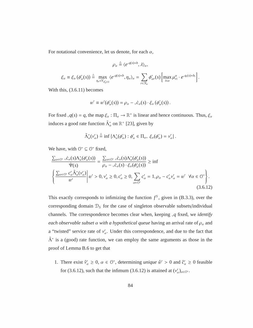
For notational convenience, let us denote, for eachα,

ρα= 〈e⋄q(s)+b, λ〉α,

ξα ≡ ξα(

φ′α(s)) = max

ηα∈Vφ′α(s)

〈e⋄q(s)+b, ηα〉α =∑

r∈Rα

φ′αr(s)[

maxi∈α

µαri · e⋄qi (s)+bi

]

.

With this, (3.6.11) becomes

w′ ≡ w′(φ′α(s)) = ρα − ⋄cα(s) · ξα(

φ′α(s))

.

For fixed⋄q(s) = q, the mapξα : Πα → R+ is linear and hence continuous. Thus,ξα

induces a good rate functionΛ∗α onR+ [23], given by

Λ∗α(ν′α)= inf

Λ∗α(φ′α) : φ′α ∈ Πα, ξα(φ′α) = ν′α

.

We have, withO∗ ⊆ O∗ fixed,∑

α∈O∗ ⋄cα(s)Λ∗α(φ′α(s))

Ψ(s)=

∑

α∈O∗ ⋄cα(s)Λ∗α(φ′α(s))

ρα − ⋄cα(s) · ξα(φ′α(s))≥ inf

∑

α∈O∗ c′αΛ∗α(ν′α)

w′

∣∣∣∣∣∣w′ > 0, ν′α ≥ 0, c′α ≥ 0,

∑

α∈O∗c′α = 1, ρα − c′αν

′α = w

′ ∀α ∈ O∗

.

(3.6.12)

This exactly corresponds to infimizing the functionf S, given in (B.3.3), over the

corresponding domainDS for the case of singleton observable subsets/individual

channels. The correspondence becomes clear when, keeping⋄q fixed, weidentify

each observable subsetα with a hypothetical queuehaving an arrival rate ofρα and

a “twisted” service rate ofν′α. Under this correspondence, and due to the fact that

Λ∗ is a (good) rate function, we can employ the same arguments asthose in the

proof of Lemma B.6 to get that

1. There exist ˆν′α ≥ 0, α ∈ O∗, determininguniquew′ > 0 andc′α ≥ 0 feasible

for (3.6.12), such that the infimum (3.6.12) is attained at (ν′α)α∈O∗.

84

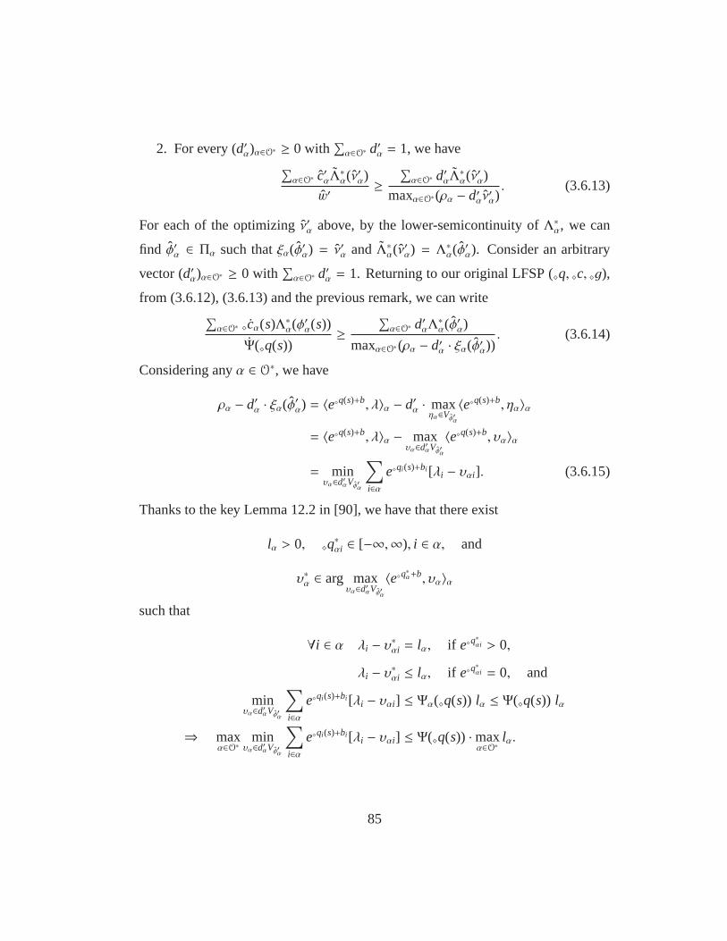
2. For every (d′α)α∈O∗ ≥ 0 with∑

α∈O∗ d′α = 1, we have∑

α∈O∗ c′αΛ∗α(ν′α)

w′≥

∑

α∈O∗ d′αΛ∗α(ν′α)

maxα∈O∗(ρα − d′αν′α). (3.6.13)

For each of the optimizing ˆν′α above, by the lower-semicontinuity ofΛ∗α, we can

find φ′α ∈ Πα such thatξα(φ′α) = ν′α andΛ∗α(ν′α) = Λ

∗α(φ′α). Consider an arbitrary

vector (d′α)α∈O∗ ≥ 0 with∑

α∈O∗ d′α = 1. Returning to our original LFSP (⋄q, ⋄c, ⋄g),

from (3.6.12), (3.6.13) and the previous remark, we can write∑

α∈O∗ ⋄cα(s)Λ∗α(φ′α(s))

Ψ(⋄q(s))≥

∑

α∈O∗ d′αΛ∗α(φ′α)

maxα∈O∗(ρα − d′α · ξα(φ′α)). (3.6.14)

Considering anyα ∈ O∗, we have

ρα − d′α · ξα(φ′α) = 〈e⋄q(s)+b, λ〉α − d′α · maxηα∈Vφ′α

〈e⋄q(s)+b, ηα〉α

= 〈e⋄q(s)+b, λ〉α − maxυα∈d′αVφ′α

〈e⋄q(s)+b, υα〉α

= minυα∈d′αVφ′α

∑

i∈αe⋄qi (s)+bi [λi − υαi]. (3.6.15)

Thanks to the key Lemma 12.2 in [90], we have that there exist

lα > 0, ⋄q∗αi ∈ [−∞,∞), i ∈ α, and

υ∗α ∈ arg maxυα∈d′αVφ′α

〈e⋄q∗α+b, υα〉α

such that

∀i ∈ α λi − υ∗αi = lα, if e⋄q∗αi > 0,

λi − υ∗αi ≤ lα, if e⋄q∗αi = 0, and

minυα∈d′αVφ′α

∑

i∈αe⋄qi (s)+bi [λi − υαi] ≤ Ψα(⋄q(s)) lα ≤ Ψ(⋄q(s)) lα

⇒ maxα∈O∗

minυα∈d′αVφ′α

∑

i∈αe⋄qi (s)+bi [λi − υαi] ≤ Ψ(⋄q(s)) ·max

α∈O∗lα.

85

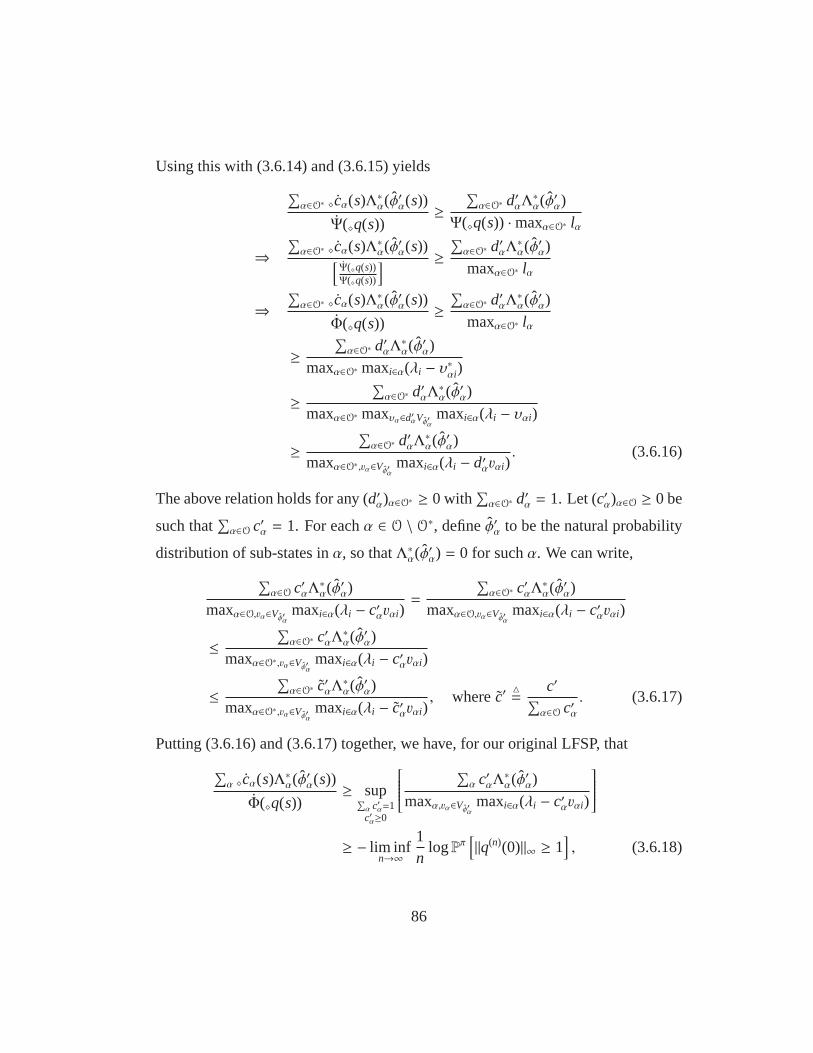
Using this with (3.6.14) and (3.6.15) yields

∑

α∈O∗ ⋄cα(s)Λ∗α(φ′α(s))

Ψ(⋄q(s))≥

∑

α∈O∗ d′αΛ∗α(φ′α)

Ψ(⋄q(s)) ·maxα∈O∗ lα

⇒∑

α∈O∗ ⋄cα(s)Λ∗α(φ′α(s))

[Ψ(⋄q(s))Ψ(⋄q(s))

] ≥∑

α∈O∗ d′αΛ∗α(φ′α)

maxα∈O∗ lα

⇒∑

α∈O∗ ⋄cα(s)Λ∗α(φ′α(s))

Φ(⋄q(s))≥

∑

α∈O∗ d′αΛ∗α(φ′α)

maxα∈O∗ lα

≥∑

α∈O∗ d′αΛ∗α(φ′α)

maxα∈O∗ maxi∈α(λi − υ∗αi)

≥∑

α∈O∗ d′αΛ∗α(φ′α)

maxα∈O∗ maxυα∈d′αVφ′αmaxi∈α(λi − υαi)

≥∑

α∈O∗ d′αΛ∗α(φ′α)

maxα∈O∗,vα∈Vφ′α maxi∈α(λi − d′αvαi). (3.6.16)

The above relation holds for any (d′α)α∈O∗ ≥ 0 with∑

α∈O∗ d′α = 1. Let (c′α)α∈O ≥ 0 be

such that∑

α∈O c′α = 1. For eachα ∈ O \ O∗, defineφ′α to be the natural probability

distribution of sub-states inα, so thatΛ∗α(φ′α) = 0 for suchα. We can write,

∑

α∈O c′αΛ∗α(φ′α)

maxα∈O,vα∈Vφ′α maxi∈α(λi − c′αvαi)=

∑

α∈O∗ c′αΛ∗α(φ′α)

maxα∈O,vα∈Vφ′α maxi∈α(λi − c′αvαi)

≤∑

α∈O∗ c′αΛ∗α(φ′α)

maxα∈O∗,vα∈Vφ′α maxi∈α(λi − c′αvαi)

≤∑

α∈O∗ c′αΛ∗α(φ′α)

maxα∈O∗,vα∈Vφ′α maxi∈α(λi − c′αvαi), wherec′

=

c′∑

α∈O c′α. (3.6.17)

Putting (3.6.16) and (3.6.17) together, we have, for our original LFSP, that

∑

α ⋄cα(s)Λ∗α(φ′α(s))

Φ(⋄q(s))≥ sup

∑

α c′α=1c′α≥0

∑

α c′αΛ∗α(φ′α)

maxα,vα∈Vφ′α maxi∈α(λi − c′αvαi)

≥ − lim infn→∞

1n

logPπ[

||q(n)(0)||∞ ≥ 1]

, (3.6.18)

86

for the stationary measurePπ of any stabilizing scheduling policy, by Theorem 3.4.

Infimizing (3.6.18) over all valid LFSPs and using Proposition 3.6 yields

J∗ ≥ − lim infn→∞

1n

logPπ[

||q(n)(0)||∞ ≥ 1]

,

which finishes the proof.

3.7 Conclusions and Future Work

For scheduling with only partial wireless Channel State Information (CSI),

we developed the Max-Exp and Max-Queue scheduling algorithms, which yield

optimal queue overflow tails. This shows that structurally simple scheduling algo-

rithms which use partial CSI can guarantee high performance.Moreover, to control

queue backlogs in such cases, no additional statistical or extraneous information is

explicitly required by the scheduling algorithms.

Future directions for research include studying scheduling with information

from general user subsets, temporally varying constraintson available CSI, and

performance under delayed CSI with time-correlated channels. Another promis-

ing line of future work is to incorporate partial channel state observability into the

many-user, small-buffer OFDMA scheduling model of [9], and investigate if itera-

tive multi-channel scheduling is possible for optimal performance.

87

Chapter 4

Coordinated Multi-cell Wireless Scheduling

4.1 Introduction

Next-generation cellular systems like 3GPP-Long Term Evolution (LTE)

[61] are based on the technique of Orthogonal Frequency Division Multiple Access

(OFDMA), and promise high-speed packet-based services fora variety of applica-

tions. In a typical downlink of such a cellular system, base stations enable multiple

mobile users to share available channel resources by assigning them different fre-

quency bands or “tones”. These tone-based channels experience temporal fluctua-

tions in quality due to fading, and these fluctuations dictate the instantaneous data

rates that can be sustained within a time slot. Base stations obtain channel quality

measurements from the mobile users attached to them, and perform resource allo-

cation, on a timescale of about every 1-2 milliseconds. Thishelps the base stations

opportunistically exploit local channel fluctuations to schedule data transmissions

to the users.

Data transmission in amulticellular environment withmany base stations

is, however, impeded by the following factors:

1. Co-channel interference:A system of several base stations is prone to inter-

cell interference, where transmissions to neighboring mobile users assigned

the same frequencies in different cells collide, resulting in a loss of through-

put. The issue of interference management is especially vital for modern

88

LTE-basedfemtocell networks[55], which comprise of many small base sta-

tions in indoor environments to improve coverage and capacity. Due to un-

planned or ad-hoc deployments, femtocell base stations suffer from radio

interference from nearby femtocells and macrocells which impacts overall

throughput. Mitigating inter-cell interference in femtocell networks has thus

been a subject of much recent research [56, 57].

2. High backhaul latency: Avoiding interference entirely demands that the

base stations coordinate their transmissions using instantaneous channel state

information acquired from other base stations. Such coordination at the time

scale of channel fluctuations, however, is rendered infeasible by the relatively

high latencies (of the order of 10s-100s of milliseconds) ofbackhaul links

that connect base stations. Femtocell base stations typically use third-party

IP/Ethernet backhauls to coordinate interfering transmissions, and are con-

strained to communicate over much slower timescales [56]. Communication

between base stations is thus limited to sharing information which is signifi-

cantly delayed compared to instantaneous channel state variations.

3. Partial local channel state information: Base stations cannot acquire even

the complete instantaneous channel states for all their ownusers. This is be-

cause OFDMA-based systems like LTE have many sub-channels,and getting

channel state information for all users on each sub-channelin every time-slot

may be prohibitive in terms of available feedback bandwidth.

In such a setting, the challenge is how to effectively use a combination of

network state information available at the base stations – (a) partial “local” infor-

mation, i.e., instantaneous channel quality estimates, gathered from users at the

timescale of channel state variations, and (b) other “global” information (such as

89

channel statistics, accumulated queue lengths, user interference patterns etc.) gath-

ered from other base stations and significantly delayed fromthe instantaneous chan-

nel state variations – and schedule for maximum throughput.

In this chapter, we consider a collection of base stations, each serving an

exclusive set of users, in a time-slotted system. To capturethe fact that certain

users may interfere (e.g. users in different cells on the same frequencies located

close to each other) while others may not (e.g. users on orthogonal channels, or on

common frequencies but far from each other), we model anarbitrary collection of

subsets of interfering users in the user population. Inter-cell interference is modeled

by assuming that transmissions to interfering users by their respective base stations

collide if scheduled simultaneously. At each time slot, each base station can access

instantaneous channel states for a subset of its users, exchange delayed information

with other base stations, and finally schedule users from thechosen subset.

With this information structure at the base stations, we first characterize the

network throughput region, i.e., the set of all long-term joint service rates achiev-

able for all users. A key observation we exploit is that common state informa-

tion provided by global delayed queues allows coupling of decisions across base

stations. We demonstrate the optimal way of using this coupled state to coordi-

nate scheduling across multiple base stations, and developa provably throughput-

optimal scheduling algorithm. In other words, when it is possible to share global de-

layed information among base stations, it is enough to sharedelayed queue lengths

to achieve throughput-optimality. To the best of our knowledge, this is the first

throughput-optimality result using the information structure of local limited instan-

taneous channel state and global delayed information (queue lengths). We also

quantify, via analysis and simulations, how the packet delay performance of our

throughput-optimal scheduling algorithm varies with the amount of delay in the

90

shared queue length information.

4.1.1 Summary of Contributions

The results in this chapter include the following:

1. We derive the throughput region of a multi-base-station system, with given

arbitrary subsets of interfering users, in which the base stations schedule us-

ing the information structure of (a) local limited channel state information,

and (b) globally shared information which is independent ofthe instanta-

neous channel states. Moreover, we show that any rate withinthe throughput

region can be obtained by timesharing across a simple class of static schedul-

ing policies. In a static scheduling policy, each base station always picks a

fixed subset of its users, and schedules each user in that subset depending

solely on its instantaneous channel state and a fixed binary vector associated

with that state.

2. We present a two-tier, distributed and provably throughput-optimal schedul-

ing algorithm that relies on the base stations sharing theirusers’ queue lengths

everyT (an integer parameter) time slots. Specifically, at everyT-th time slot,

all the base stations communicate their queue lengths to each other. For the

next T time slots, each base station uses this (delayed) queue length infor-

mation, along with knowledge about channel statistics and interfering users,

to locally observe an appropriate subset of its channels’ states and schedule

the corresponding users. The parameterT in our algorithm is the maximum

“staleness” of exchanged queue length information, and is also a measure of

the inter-base-station coordination time. Moreover, the scheduling algorithm

is throughput-optimal foranyfixed value ofT, meaning that the coordination

91

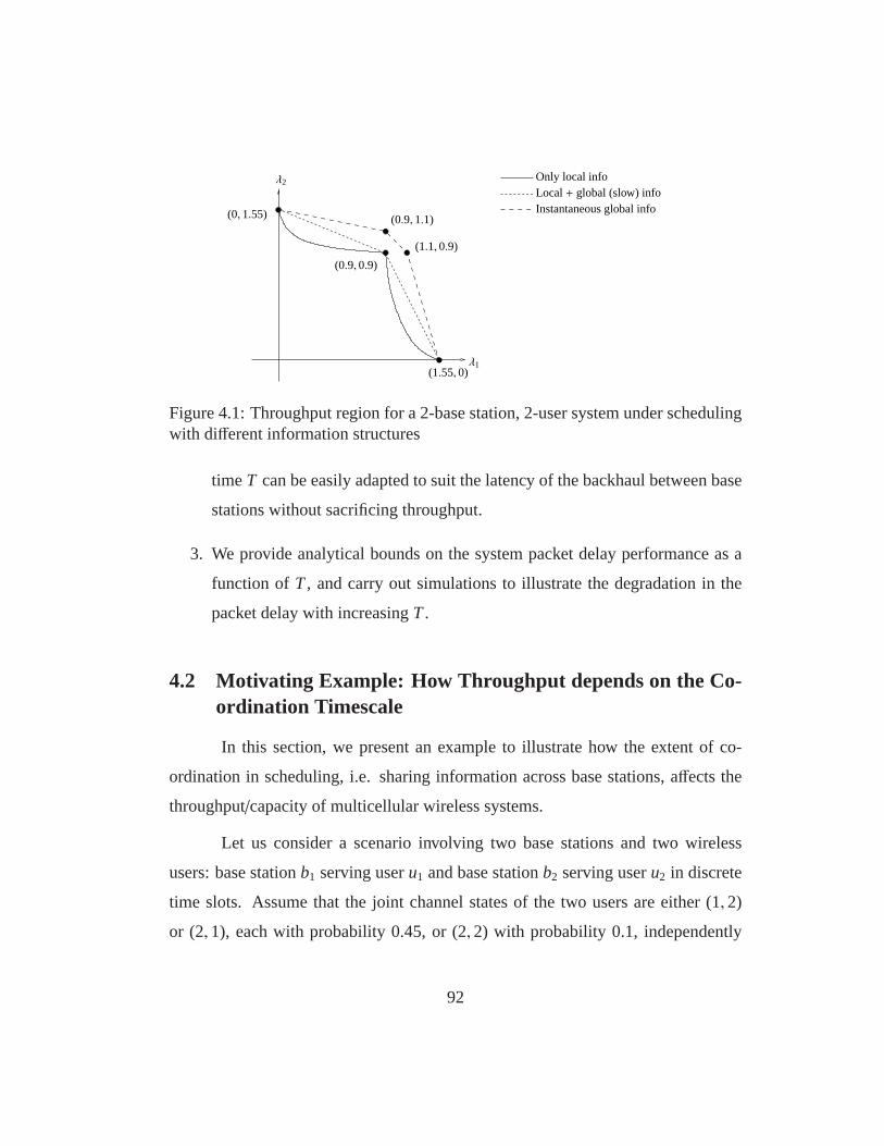
Instantaneous global info

λ1(1.55, 0)

λ2

(0, 1.55) (0.9, 1.1)

(0.9, 0.9)

(1.1, 0.9)

Local+ global (slow) infoOnly local info

Figure 4.1: Throughput region for a 2-base station, 2-user system under schedulingwith different information structures

timeT can be easily adapted to suit the latency of the backhaul between base

stations without sacrificing throughput.

3. We provide analytical bounds on the system packet delay performance as a

function of T, and carry out simulations to illustrate the degradation inthe

packet delay with increasingT.

4.2 Motivating Example: How Throughput depends on the Co-ordination Timescale

In this section, we present an example to illustrate how the extent of co-

ordination in scheduling, i.e. sharing information acrossbase stations, affects the

throughput/capacity of multicellular wireless systems.

Let us consider a scenario involving two base stations and two wireless

users: base stationb1 serving useru1 and base stationb2 serving useru2 in discrete

time slots. Assume that the joint channel states of the two users are either (1,2)

or (2,1), each with probability 0.45, or (2,2) with probability 0.1, independently

92

in each time slot. The channel state denotes how many packetscan be transmitted

to the user in the event of a successfully scheduled transmission. Corresponding

to the situation in an LTE system where the two users are assigned the same fre-

quencies and are located close to each other at the cell boundary, we assume that

transmissions to these two users collide if scheduled together. At every time slot,

each base station decides whether to schedule its respective user or not depend-

ing on the structure of network state information it possesses. We consider three

possible structures of network state information:

1. First, assume that at every time slot, each base station knows only its own

user’s current channel state (i.e., the base stations havelocal channel state in-

formation with no coordination). In this case we can show that the throughput

region is enclosed by the solid curved lines connecting the points (0,1.55),

(0.9,0.9) and (1.55,0) in Fig. 4.1. Essentially, this is equivalent to saying that

each base station decides independently to schedule its ownuser with some

fixed probability. The first (resp. third) point represents the case when user

u1 (resp.u2) is always scheduled and the other user is always not scheduled.

The second point represents the case when each user is scheduled if and only

if its observed channel state is 2.

2. Next, assume again that each base station knows only its own user’s cur-

rent channel state, but that the base stations can exchange delayed or slowly

varying information – more specifically, any information independent of their

users’ current channel states. This models the fact that backhaul capabilities

between the base stations do not permit exchange of instantaneous channel

state information occurring on a fast timescale. For instance, the base stations

can rely on a source of common randomness to make their scheduling deci-

sions. This is the situation in which the base stations havelocal channel state

93

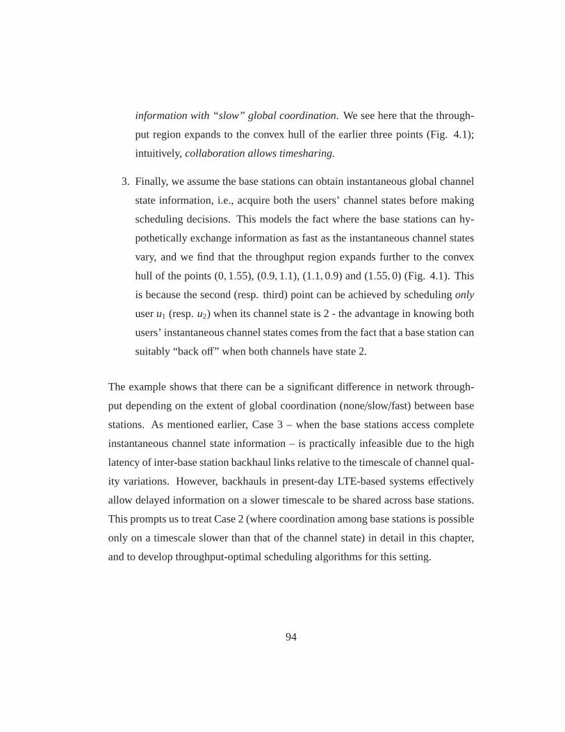
information with “slow” global coordination. We see here that the through-

put region expands to the convex hull of the earlier three points (Fig. 4.1);

intuitively, collaboration allows timesharing.

3. Finally, we assume the base stations can obtain instantaneous global channel

state information, i.e., acquire both the users’ channel states before making

scheduling decisions. This models the fact where the base stations can hy-

pothetically exchange information as fast as the instantaneous channel states

vary, and we find that the throughput region expands further to the convex

hull of the points (0,1.55), (0.9,1.1), (1.1,0.9) and (1.55,0) (Fig. 4.1). This

is because the second (resp. third) point can be achieved by schedulingonly

useru1 (resp.u2) when its channel state is 2 - the advantage in knowing both

users’ instantaneous channel states comes from the fact that a base station can

suitably “back off” when both channels have state 2.

The example shows that there can be a significant difference in network through-

put depending on the extent of global coordination (none/slow/fast) between base

stations. As mentioned earlier, Case 3 – when the base stations access complete

instantaneous channel state information – is practically infeasible due to the high

latency of inter-base station backhaul links relative to the timescale of channel qual-

ity variations. However, backhauls in present-day LTE-based systems effectively

allow delayed information on a slower timescale to be sharedacross base stations.

This prompts us to treat Case 2 (where coordination among basestations is possible

only on a timescale slower than that of the channel state) in detail in this chapter,

and to develop throughput-optimal scheduling algorithms for this setting.

94

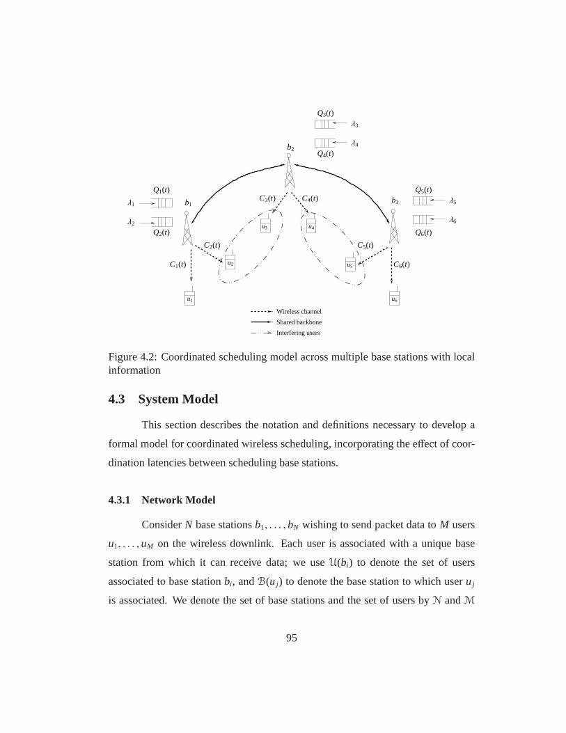
u4

λ4

λ3

Q3(t)

Q4(t)b2

b1b3

C5(t)

C6(t)

λ1

λ2

λ5

λ6

Q1(t)

Q2(t)

Q5(t)

Q6(t)

C3(t) C4(t)

C2(t)

C1(t)

Wireless channel

Shared backbone

Interfering users

u1 u6

u2

u3

u5

Figure 4.2: Coordinated scheduling model across multiple base stations with localinformation

4.3 System Model

This section describes the notation and definitions necessary to develop a

formal model for coordinated wireless scheduling, incorporating the effect of coor-

dination latencies between scheduling base stations.

4.3.1 Network Model

ConsiderN base stationsb1, . . . ,bN wishing to send packet data toM users

u1, . . . ,uM on the wireless downlink. Each user is associated with a unique base

station from which it can receive data; we useU(bi) to denote the set of users

associated to base stationbi, andB(uj) to denote the base station to which useruj

is associated. We denote the set of base stations and the set of users byN andM

95

respectively.

4.3.2 Arrival and Channel Model

Time is slotted into discrete units. Data packets destined for useruj ∈ U(bi)

arrive at base stationbi as a stationary nonnegative integer-valued random process

Aj(t), t = 1,2, . . .. For simplicity we will assume thatAj(t) is independent and iden-

tically distributed (iid)over time slotst with E[Aj(t)] = λ j, andAj(t) ≤ Amax. Let

A(t)= (A1(t), . . . ,AM(t)). Packets get queued if they are not immediately transmit-

ted. The channel between useruj and its associated base station is time-varying,

and we assume that its state stays constant for the duration of a time slot. We

denote the channel state random process byC j(t), t = 1,2, . . ., where for anyj,

C j(t) takes values in a finite setC. We explicitly assume thatC consists of the

integers 0≤ c1 < c2 < · · · < cK = Cmax. The aggregate channel state pro-

cessC(t)= (C j(t) : j = 1, . . . ,M) is assumed to beiid over time slots, but the

channel states can be correlated across users. For a subsetW ⊆ u1, . . . ,uM of

users, we overload notation and denote byCW(t) the channel state of just the sub-

setW. Let π(·) denote the probability mass function of the aggregate channel state

(C1(t), . . . ,CM(t)), i.e.,π(r1, . . . , rM)= P[C1(t) = r1, . . . ,CM(t) = rM], with r i ∈ C

for all i. Such a canonical wireless system is shown in Fig. 4.2.

4.3.3 Queueing Model

Each base stationbi maintains one packet queue for every useruj associated

with it, into which data packets destined touj get buffered if they are not immedi-

ately transmitted. We denote the fact that useruj ∈ U(bi) is successfully scheduled

for data reception at time slott by setting a binary random variableD j(t) = 1. When

this happens, up toC j(t) packets can be drained from its packet queue. Thus ifQ j(t)

96

denotes the queue-length process for the packet queue of user uj, then the evolution

of Q j can be described as

Q j(t + 1) = maxQ j(t) − D j(t)C j(t),0 + Aj(t). (4.3.1)

Another form of (4.3.1) which we use later is

Q j(t + 1) = Q j(t) + Aj(t) − E j(t), (4.3.2)

whereE j(t)= minD j(t)C j(t),Q(t). Let Q(t) represent the vector of queue lengths

(Q1(t), . . . , QM(t)) at time slott.

4.3.4 Multiple Base Station Scheduling Model

In the multiple base station network, at every time slott, each base station

bi schedules transmissions for a set of its users. Following the motivating example,

we model the information structure that each base station uses to schedule users as

having two important properties:

1. Limited, local channel state information at base stations: Each base sta-

tion accesses instantaneous channel state information foronly asubsetof its

users prior to scheduling. We let each base stationbi choose a subsetObi (t) of

its users at every time slott, from a fixed arbitrary collectionO(bi) of subsets

of U(bi). Following this, the instantaneous stateCObi (t)(t) of the chosen users’

channels is available tobi, and it can use this knowledge to schedule users

in Obi (t). We use a binary random variableBi(t) to represent whether a user

i ∈ Obi (t) is scheduled at timet (Bi(t) = 1 denotes thati is scheduled). This

framework formally captures the fact that channel state feedback capabilities

between base stations and their users are potentially limited.

97

2. Delayed, slower-timescale coordination between base stations: Base sta-

tions can share information to help coordinate scheduling,but instantaneous

channel state information at each time slot cannot be shared. This captures

the fact that the backhaul links that allow base stations to communicate suffer

from a high latency relative to the timescale of channel state variation.

To model this formally, we first fix a sufficiently large integerR> 0 which we

will call the systemhistory parameter. At time slot t, we assume that each

base station can access the history of the entire network – queue lengths,

channel states, arrivals – for all the previousR time slots up to andnot in-

cluding t, denoted by the (random) vectorHR(t)= (Q(t − R), . . . ,Q(t),C(t −

R), . . . ,C(t − 1),A(t −R), . . . ,A(t − 1)). This says that the backhaul coordina-

tion links are capable of letting the base stations share their past observations

with each other; however, any instantaneous (at timet) channel state infor-

mation cannot be propagated within the same time slot. We remark that the

restriction of available system history to the previousR time slots is made for

technical convenience – our results hold when, for instance, the entire system

history (past channel states, scheduling decisions and arrivals) is available at

the base stations.

At each time slott, in addition to the system historyHR(t), we assume that all

the base stations can utilizecommon randomness, represented by a random

variableG(t) that is independent from the instantaneous channel state C(t).

The independence ofG(t) from the instantaneous channel state is in keeping

with the constraint that base stations are incapable of sharing instantaneous

channel state information among themselves.G(t) represents any common,

auxiliary information which can be used by all the base stations. For in-

stance,G(t) can denote measured channel/arrival/queue statistics, or just a

98

current time index that drives time-dependent scheduling,or the outcome of

a common “coin toss” sequence to timeshare across base stations etc. It mod-

els common information that can be propagated across the inter-base station

backhaul in order to coordinate scheduling (we discuss thisin detail in Sec-

tion 4.4 in the context of time-sharing policies).

Thus, the total information available to the base stations at each time slott,

as a result of slow coordination over the backhaul, isXR(t)= (HR(t),G(t)),

which we call thesystem state.

In summary, every base station first picks a subset of its users to observe

their instantaneous channel states – this can depend on queue lengths, channel

states, arrivals and auxiliary information in the lastR slots. After having observed

the instantaneous channel states for that subset, the base station schedules users in

the subset depending on their instantaneous channel statesand the global informa-

tion it already possesses. We term the collective set of rules applied at each time

slot by every base station to schedule users as thescheduling policy or algorithm

used by the base stations.

4.3.5 Interference Model

As introduced earlier, data transmissions to users in different cells that are

close to each other and use the same frequencies are prone to interference. At the

same time, transmissions to users on suitably orthogonal channels (e.g. different

frequencies or tones in an OFDMA-based system) can occur simultaneously with-

out any interference. For each useruj ∈ M, let I(uj) ⊂ M denote the set of users

that interfere withuj, meaning that useruj cannot receive any data packets in a time

slot at which a user inI(uj) is scheduled. We assume thatuj < I(uj) for all j. For

99

instance,I(uj) = ∅ means that useruj does not experience interference from any

other user. Thus, we have, for all usersuj,

D j(t) = Bj(t)∏

uk∈I(u j )

(1− Bk(t)). (4.3.3)

With this, the maximum number of packets that can be drained from the queue for

useruj at timet becomes

F j(t)= C j(t)D j(t). (4.3.4)

Such a collision interference model together with the “GO/NO-GO” type

scheduling model described earlier models a rudimentary “binary” power-control

scheme for users in the network.

4.3.6 Objective/Performance Metric

For the setup described above, note that under any scheduling policy, the

system stateXT(t) is a discrete time Markov chain. Let us assume that this Markov

chain is irreducible and aperiodic1. Following standard terminology, we say that a

vector of arrival ratesλ = (λ1, . . . , λM) with λi ≥ 0, i = 1, . . . ,M is supportedby a

scheduling policy if the Markov chainXT(t) is positive recurrent under the policy

when the packet arrival rates at the user queues areE[A j(t)] = λ j, j = 1 . . . ,M

(this corresponds to the intuitive notion that the queues inthe network are drained

as fast as they fill up, i.e., they arestable). The goal is then to characterize the

1This can, for example, be satisfied if the arrival and channelprocess marginal distributionshave positive probability on a finite subset of the non-negative integer lattice0,1, ..., L. Weakerconditions suffice by using different notions of stability, e.g., that there is a non-empty positiverecurrent set of states, and an associated finite subset which is entered in finite time with probabilityone [4]. However, to avoid purely technical complications,we assume that the support of the arrivaland channel state processes are such that the scheduling policies we consider render the MarkovChain to be aperiodic and irreducible (see also Section 3 in [27])

100

stability region, which we define to be the set of all vectors of arrival rates (λ j :

j = 1, . . . ,M) supported by at least one scheduling policy. In addition, we wish to

investigate whether there exists asingle scheduling policywhich can supportany

arrival rate vector in the stability region – a property we call throughput optimality

of a scheduling policy.

4.4 The Stability Region with Slow Global Coordination

In this section, we explicitly characterize the stability region of a system

of base stations that schedule users with coordination and limited local channel

state information. We first introduce a class ofstatic scheduling policies, called

Static Service Split (SSS)policies, which use only instantaneous local channel state

information at each base station to make scheduling decisions. SSS policies can

achieve a finite set of rates in the stability region, and by using additional common

randomness (e.g., a common sequence of coin toss outcomes),the base stations

can suitably time-share across SSS policies. We show in Theorem 4.1 that the

stability region is, in fact, the convex hull that results from all the possible time-

sharing combinations of SSS policies. In other words, any given scheduling policy

is similar, in the sense of long-term service rates, to aStatic Time-sharing (STS)

policy, or a time-shared combination of SSS policies.

4.4.1 SSS Policies

Let us consider a class of “simple” scheduling policies which, inspired by

[4], we will term Static Service Split(SSS) policies. However, unlike the standard

SSS policies used in literature for scheduling with complete channel state informa-

tion [4, 83], our SSS policies are essentially “two-tiered”, and are specifications

of both (i) fixed subsets that base stations must always pick and(ii) fixed “binary

101

vectors” for every observed subset channel state, that indicate exactly which users

must be scheduled when that channel state is observed.

Formally, an SSS policyP is defined by a tupleP = (W1, . . . ,WN, z1, . . . , zN),

where for eachi, Wi is a permissible subset of users for base stationbi, andzi is a col-

lection of binary length-|Wi | vectors, one for each possible set of observed channel

states of users inWi. Equivalently, we can think ofzi as a map that takes the chan-

nel statesCWi (t) observed for subsetWi into a binary vectorzi(CWi (t)) ∈ 0,1|Wi |.

Scheduling using the SSS policyP is carried out as follows. At each time slott,

1. Each base stationbi picks afixedsubsetObi (t) = Wi of its users in order to

observe their instantaneous channel states.

2. All the users forbi not in Wi are not scheduled, i.e.,Bj(t) = 0 for such users.

A user uj in Wi is scheduled if and only if (zi(CWi (t))) j = 1, i.e., Bj(t) =

(zi(CWi (t))) j.

Thus, an SSS policy only specifies “local” scheduling rules per base station: each

base station uses channel-state information from a predefined subset of users and

schedules users in the subset accordingly. Note that scheduling decisions among

different base stations are functions purely of the instantaneous channel states of

their respective users, and are not coupled by any other common/shared informa-

tion. In what follows, we introduce a more general class of scheduling policies

calledStatic Time-sharing policies, which involve the base stations time-sharing

between SSS policies using a common randomness sequenceG(t)t.

4.4.2 Static Time-sharing Policies

A Static Time-sharing (STS)policy results when base stations use common

randomness to time-share between SSS policies. It is parameterized by a finite set

102

of SSS policies (Pi)Ki=1, together with a corresponding set of nonnegative weights

(φi)Ki=1 that sum to 1. At each time slott, independent of previous time slots, all

the base stations together decide to schedule according to the SSS policyPi with

probabilityφi. This can be achieved, if, for instance, the base stations use a com-

mon random sequenceG(t)t where eachG(t) ∈ 1,2, . . . ,K is the outcome of an

independentK-sided coin-toss with probability distribution (φi)Ki=1, and indexes the

SSS policyφG(t) for time slott. Thus, in an STS policy, scheduling decisions among

different base stations are coupled not only through their users’ instantaneous chan-

nel states, but also via the common randomness that they use.In the next section,

we will see that STS policies can achieve all rates in the convex hull of the rates of

SSS policies (i.e., the “corner point rates”), and moreover, that no scheduling policy

limited by a high-latency backhaul can stabilize rates outside this convex hull.

4.4.3 Characterization of the Stability Region

Towards an explicit characterization of the stability region with slow/high-

latency backhauls, let us define therate vectorµP associated with an SSS policyP.

For each useruj, as in (4.3.4), let

FP

j (t)= C j(t)D

P

j (t),

whereDP

j (t) is simplyD j(t) from (4.3.3) but with the superscriptP indicat-

ing explicit dependence on the scheduling policyP. Next, letµP = (µP

1 , . . . , µP

M),

where

µP

j= E[FP

j (t)]

=∑

r≡(r1,...,rM)

π(r1, . . . , rM) r j(

zi(r |Wi ))

j

∏

uk∈I(u j )bl=B(uk)

(1− (

zl(r |Wl ))

k). (4.4.1)

103

Observe thatµP

j represents the vector of long-term, ergodic service rates that

the SSS policyP delivers to the flows to all the users in the system. In a similar

manner, ifP is an STS policy, i.e.,P is a combination of SSS policies (P1, . . . ,PK)

with weightsφ1, . . . , φK, then we define the rate vectorµP = (µP

1 , . . . , µP

M) associated

with P by

µP

j=

K∑

i=1

φiµPij . (4.4.2)

Essentially, the rate vector for an STS policy is defined to bethe convex

combination of the rate vectors of its component SSS policies.

For an SSS policyP with rate vectorµP, all arrival rate vectorsλ = (λ1, . . . , λM)

, with λi ≥ 0, i = 1, . . . ,M, that are dominated byµP lie in the system stability re-

gion, since the scheduling policyP stabilizes them. Furthermore, any arrival rate

vector that is the convex combination of SSS policy rate vectors also belongs to

the stability region, since an appropriate STS policy corresponding to the convex

combination stabilizes it. If we let

R= int Co(µP : P an SSS policy) = int µP : P an STS policy,

then the preceding argument indicates thatR is definitely aninner bound to the sta-

bility region (recall that the stability region consists ofall those arrival rate vectors

which can be supported bysomescheduling policy). Theorem 4.1 below states that

in fact, the stability region is no more thanR:

Theorem 4.1. The stability region of the system isR, i.e., a vector of arrival rates

λ = (λ1, . . . , λM) with λi ≥ 0, i = 1, . . . ,M is supported by a scheduling policy if

and only ifλ ∈ R.

104

C2(t)

Shared backbone

Interfering users

Wireless channel

b2 λ2

λ3

Q2(t)

Q3(t)

b1

λ1

Q1(t)

u1

u3

u2C1(t)

C3(t)

Figure 4.3: Stability region example: Three-user, Two-base-station System withslow coordination between the base stations

This result says that any scheduling policy which stabilizes the system for a

certain choice of arrival rates effectively behaves like an STS policy, i.e., a suitable

time-shared combination of SSS scheduling policies, in thesense of the long-term

service rates it delivers. This result is useful later, in Section 4.5, towards showing

that a particular scheduling algorithm we develop is throughput-optimal. The proof

of this theorem is similar in spirit to the results in [4, 108,109] used to characterize

the stability region. It uses the fact that a system stable/ergodic under a policy must

have consistent long-term fractions, which are in turn usedto construct STS policies

yielding the same service rates. Refer to Appendix C.1 for the proof.

4.4.4 Example: Stability Region for a Three-user, Two-base-station System

To illustrate the concepts and result of the previous section, let us derive the

stability region for a simple case of two base stationsb1 andb2 serving a total of

three usersu1,u2,u3. u1 is associated tob1 whereasu2 andu3 are associated tob2.

Channel states for all the three users are either 0 or 1 (ON/OFF channels). Consider

the case when all the users are in geographic proximity to each other and have

105

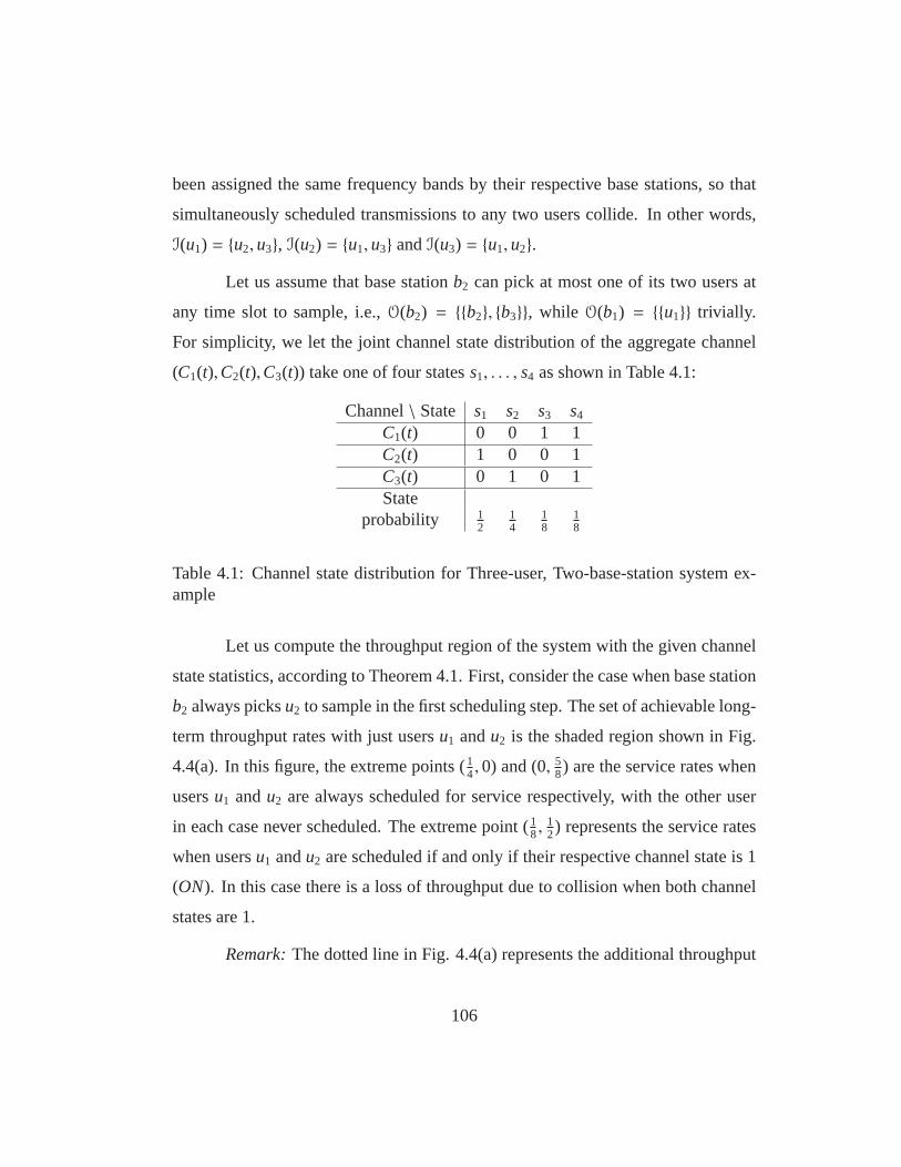
been assigned the same frequency bands by their respective base stations, so that

simultaneously scheduled transmissions to any two users collide. In other words,

I(u1) = u2,u3, I(u2) = u1,u3 andI(u3) = u1,u2.

Let us assume that base stationb2 can pick at most one of its two users at

any time slot to sample, i.e.,O(b2) = b2, b3, while O(b1) = u1 trivially.

For simplicity, we let the joint channel state distributionof the aggregate channel

(C1(t),C2(t),C3(t)) take one of four statess1, . . . , s4 as shown in Table 4.1:

Channel\ State s1 s2 s3 s4

C1(t) 0 0 1 1C2(t) 1 0 0 1C3(t) 0 1 0 1State

probability 12

14

18

18

Table 4.1: Channel state distribution for Three-user, Two-base-station system ex-ample

Let us compute the throughput region of the system with the given channel

state statistics, according to Theorem 4.1. First, consider the case when base station

b2 always picksu2 to sample in the first scheduling step. The set of achievable long-

term throughput rates with just usersu1 andu2 is the shaded region shown in Fig.

4.4(a). In this figure, the extreme points (14,0) and (0, 5

8) are the service rates when

usersu1 andu2 are always scheduled for service respectively, with the other user

in each case never scheduled. The extreme point (18,

12) represents the service rates

when usersu1 andu2 are scheduled if and only if their respective channel state is 1

(ON). In this case there is a loss of throughput due to collision when both channel

states are 1.

Remark:The dotted line in Fig. 4.4(a) represents the additional throughput

106

(14,

12)

(14, 0)

(0, 58)

λ1

λ2

(18,

12)

(18,

58)

(a)

(14,

14)

λ1

λ3

(0, 38)

(14, 0)

(18,

14)

(18,

38)

(b)

(0, 0, 38)

λ3 λ1

λ2

(18,

12, 0)

(14, 0, 0)

(0, 58, 0)

(18, 0,

14)

(c)

Figure 4.4: (a) Stability region for usersu1 andu2, (b) Stability region for usersu1

andu3, (c) Stability region for all three users

obtained when both base stations can see the channel states of both u1 andu2 before

scheduling. This helps reduce collisions when both the channels have state 1 and

hence increases throughput.

Similarly, we can compute the set of service rates when base station b2

always picksu3. The set of achievable long-term throughput rates with justusersu1

andu3 is the shaded region shown in Fig. 4.4(b). Here again, we see three extreme

points on the “northeast” boundary of the region, having similar interpretations as

in the previous figure. Also, the dotted line represents throughput gained if both

base stations know the joint channel states ofu1 andu3 before scheduling.

Theorem 4.1 now tells us that the stability region of the system can be found

by taking the convex hull of the two “sub”-rate regions we found earlier. This is

depicted graphically as the shaded region in Fig. 4.4(c).

107

4.5 Throughput-optimal Scheduling with Slow Global Coordi-nation

The result of Theorem 4.1 characterizes the network stability region as the

long-term service rates of static timesharing scheduling policies. However, observe

that

• Any given static timesharing policy is not throughput-optimal, since the set

of arrival rates stabilizable by the policy is merely the “cube” of points that

are dominated in every coordinate by its long-term service rates, and not the

whole stability region.

• For any arrival rate in the stability region, stabilizing the queueing system

with an appropriate static timesharing scheduling policy requires knowledge

of the arrival rate. In other words, the static timesharing policies that stabilize

the system for a given arrival rate explicitly depend on the arrival rate. This

motivates the need for a throughput-optimal scheduling algorithm that, for

anyarrival rate in the stability region, keeps all queues stable.

In this section, we focus on developing athroughput-optimalinformation

exchange and scheduling algorithm in which base stations share delayed queue

length information among themselves, and use this information to select local SSS

policies.

4.5.1 A Throughput-optimal Scheduling Algorithm with Slow Global Coor-dination

The scheduling algorithmPT that we describe here uses an integer parame-

ter T > 0, which represents the time interval (in slots) between successive commu-

nication exchanges between the base stations. Specifically, the algorithm operates

108

in successive epochs ofT time slots, and requires that all the queue lengths in the

system be shared globally across the base stations at the beginning of each epoch.

Thus, the timescale at which the base stations exchange queue length information

for coordinating their scheduling actions is once everyT time slots. The scheduling

policy PT is as described in Algorithm 5, and essentially operates as follows:

1. Each base station accesses the global vector of queue lengths everyT slots.

2. The global vector of queue lengths time slotkT is used to choose a “tem-

porally local” SSS policy for the nextT time slots. The subsets and binary

decision vectors for this local SSS policy are chosen in sucha way as to

maximize the sum of service rates delivered to each queue weighted by its

corresponding delayed queue length.

Note that when the history parameterR is at leastT, the scheduling al-

gorithm PT formally makes the state processXT(t)t=0,1,... a time-inhomogeneous

Markov chain, since within each scheduling epoch, the queuelengths used as weights

in (4.5.1) depend on how far into the epoch the algorithm is operating. To keep the

presentation clear, we avoid such technicalities and deal,instead, with the system

state sampled at the start of every epochXT(kT)k=1,2,..., which is a homogeneous

Markov chain under the algorithmPT .

Our next result – Theorem 4.2 – establishes two key properties of the algo-

rithm PT:

1. Throughput-optimality: The scheduling policyPT is throughput-optimal

for any fixed value of T, i.e., it can support any arrival rateλ in the stability

regionR.

109

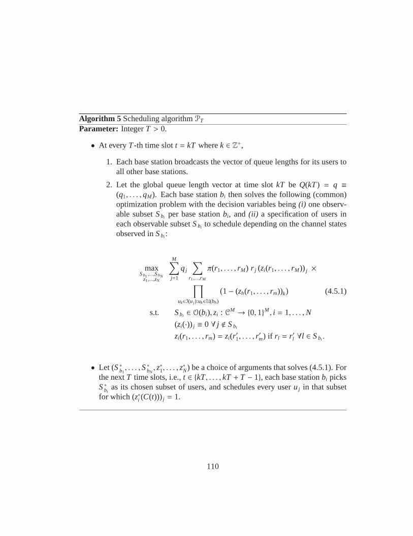
Algorithm 5 Scheduling algorithmPT

Parameter: IntegerT > 0.

• At everyT-th time slott = kT wherek ∈ Z+,

1. Each base station broadcasts the vector of queue lengths for its users toall other base stations.

2. Let the global queue length vector at time slotkT be Q(kT) = q ≡(q1, . . . ,qM). Each base stationbi then solves the following (common)optimization problem with the decision variables being(i) one observ-able subsetSbi per base stationbi, and (ii) a specification of users ineach observable subsetSbi to schedule depending on the channel statesobserved inSbi :

maxSb1 ,...,SbN

z1,...,zN

M∑

j=1

qj

∑

r1,...,rM

π(r1, . . . , rM) r j (zi(r1, . . . , rM)) j ×

∏

uk∈I(u j ):uk∈U(bh)

(

1− (zh(r1, . . . , rm))k)

(4.5.1)

s.t. Sbi ∈ O(bi), zi : CM → 0,1M, i = 1, . . . ,N

(zi(·)) j ≡ 0 ∀ j < Sbi

zi(r1, . . . , rm) = zi(r′1, . . . , r

′m) if r l = r ′l ∀l ∈ Sbi .

• Let (S∗b1, . . . ,S∗bN

, z∗1, . . . , z∗N) be a choice of arguments that solves (4.5.1). For

the nextT time slots, i.e.,t ∈ kT, . . . , kT + T − 1, each base stationbi picksS∗bi

as its chosen subset of users, and schedules every useruj in that subsetfor which (z∗i (C(t))) j = 1.

110

2. Packet-delays underPT are linear in T: The average queue lengths in the

system, under the scheduling algorithmPT , grow at most linearly with the

information lagT. As a result, by Little’s Law, the average packet delays

are linear in the average queue lengths for fixed arrival rates, and hence also

grow at most linearly inT. Indeed, the parameterT models the lag or de-

lay incurred by the base stations in exchanging queue lengthinformation,

and with an increasing information lagT, queueing delays seen by incoming

arrivals grow. Theorem 4.2 result helps quantify this intuition precisely by

giving anO(T) average queue length bound.

Theorem 4.2.For a fixed T> 0, if the arrival rateλ ∈ R, then under the scheduling

algorithmPT ,

1. XT(kT)k is a positive-recurrent Markov chain,

2. There exists a constantα > 0, not depending on T, such that under the sta-

tionary distribution ofXT(kT)k,

Eπ

M∑

j=1

Q j(lT )

≤ αT ∀l. (4.5.2)

(Eπ denotes the expectation under the stationary distributionof XT(kT)k.)

We have seen earlier – in Section 4.4 and Theorem 4.1 – that scheduling

using SSS policies can only achieve finitely many extreme points of the stability

region; additional common randomness is required to stabilize the entire through-

put region via time-sharing across SSS policies. What Theorem 4.2 shows is that

this crucial role of global, common randomness can be playedby delayed/slow-

timescale queue-length information shared among base stations during the oper-

ation of the scheduling algorithmPT. The delayed queue-length updates help to

111

correctly couple the base stations’ local SSS scheduling decisions, so as to achieve

the right time-sharing combination and stabilize any validarrival rate. This is rem-

iniscent of the manner in which queue length information is used in a distributed

fashion by Ying and Shakkottai [110] for transmission contention over interfer-

ing collision channels to achieve throughput-optimality.However, their work does

not investigate a two-time-scale information structure (i.e., slower, delayed back-

haul information and faster, instantaneous channel statesrestricted to base stations),

whereas our model addresses both (a) delayed inter-base station coordination and

(b) the issue of choosing subset-based partial channel state information at each base

station.

The proof of Theorem 4.2 relies on the key observation that delayed queue

length information in the optimization (4.5.1) helps to pick out the “right” set of

contending base stations so that, even when collisions occur within each epoch ofT

time slots, the base stations’ decisions are time-shared toensure theT-slot negative

drift of a quadratic Lyapunov function of the queue lengths.At the same time, since

each base station can access only partial, subset-based channel state information

from its users, we employ techniques from scheduling with subset-based CSI [37] to

show that the “correct” observable subsets are picked and time-shared by every base

station so as to locally achieve the right service rates. Theresults in the above work

[37] solve the problem of choosing partial, subset-based channel state information

at a lone base station for throughput-optimality; however,in this paper we face

and overcome the novel challenge of simultaneously combining (a) partial channel

state information at every base station with (b) global delayed queue-length updates

across different base stations, for achieving throughput-optimalityin the presence

of inter-cell interference.

112

We show the negative drift of the quadratic Lyapunov function underPT by

proving that

1. TheT-slot drift underPT is of the same form as that under a static time-

sharing scheduling policy, and

2. BecausePT solves the optimization (4.5.1) at everyT-th time slot, its localT-

slot drift is the most negative (and bounded away from zero) across all static

time-sharing policies.

Finally, the queue-length bound in (4.5.2) is obtained fromthe negativeT-slot Lya-

punov drift by using a technique due to Neely [65]. The readeris referred to Ap-

pendix C.2 for the complete proof of the theorem.

4.6 Simulation Results: Impact ofT on Packet Delays underPT

In this section we present simulation results that illustrate the impact of the

coordination delayT and system load (i.e., how close the arrival rate vector is to

the boundary of the throughput region) on the average delay experienced by arriving

packets, under the scheduling algorithmPT.

4.6.1 Simulation Setup

The network model we consider for the purpose of simulation is the one

presented and discussed in Section 4.4.4. As per the throughput region of the system

shown in Fig. 4.4(c), consider the rate vectorλ = ( 116,

14,

316) which is the midpoint

of the edge joining the corner points (18,

18,0) and (0,0, 3

8), and on the boundary of

the throughput region. For a scaled versionλǫ = (1− ǫ)λ, we say thatλǫ represents

a “load” of 1− ǫ to the system, analogous to the terminology used in describing

113

load in anM/M/1 queue. Arrivals are generated in aniid Bernoulli fashion and

scheduling is performed using theT-slot throughput-optimal policies developed in

Section 4.5. We examine the average delay or waiting time experience by packets

that enter the network, in the following two cases:

4.6.2 Effect of Coordination Delay

For five different loads to the system (0.55 to 0.95 in steps of 0.1), the impact

of varying the coordination intervalT from 1 to 100 on the packet delay is as shown

in Fig. 4.5. We observe that the growth in average packet delay is linear withT

which is in accordance with the result of part 2 of Theorem4.2, since by Little’s law

the average delay in the network is proportional to the average queue lengths for a

fixed net arrival rate.

4.6.3 Effect of Load

For five different values of coordination interval (T = 1, T = 10, T = 50,

T = 100 andT = 150), we plot the average packet delay in the system versus load

increasing from 0.5 towards 1. The increase in average packet delay is observed to

be particularly severe as the load approaches 100%.

4.7 Conclusions and Future Work

We considered multi-base-station wireless downlink scheduling with slow

global coordination and limited, local channel state information. We character-

ized the network stability region under this information structure, and developed

a throughput-optimal distributed scheduling algorithm inwhich it is sufficient for

base stations to share delayed queue lengths on a slow timescale to pick appropri-

114

0 10 20 30 40 50 60 70 80 90 1000

10

20

30

40

50

60

70

80

90

Coordination Delay

Ave

rage

Pac

ket D

elay

load = 0.55load = 0.65load = 0.75load = 0.85load = 0.95

Figure 4.5: Plot of average packet delay with lagT for various loads

ate subsets of users, and use the locally observed channel states of these users to

make good scheduling decisions. In this way, coordination between the base sta-

tions on a slow timescale – in the form of delayed queue lengths – helps solve the

subset-selection problem at each base station and, together with the right rules for

scheduling users in those subsets, achieves throughput-optimality. We also inves-

tigated the impact of the delay in shared queue length information on the average

packet delay performance of the system.

Future directions of research include:(i) evaluating the throughput perfor-

mance of greedy, low-complexity scheduling strategies, and (ii) refining packet de-

lay estimates using large-deviations/heavy-traffic analysis.

115

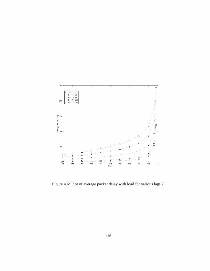
0.5 0.55 0.6 0.65 0.7 0.75 0.8 0.85 0.9 0.95 10

50

100

150

200

250

Load

Ave

rage

Pac

ket D

elay

T = 1T = 10T = 50T = 100T = 150

Figure 4.6: Plot of average packet delay with load for various lagsT

116

Chapter 5

Conclusions

This thesis, through its algorithms and results, serves to highlight the value

of network state information for scheduling in wireless systems. An important

theme that runs throughout is that the information structure available when schedul-

ing influences the capacity and performance of the system in akey manner. When

a limited portion of the overall state is used or shared, a judicious choice of the

portion to sample is required to ensure good scheduling performance.

When scheduling wireless users using backlogs and channel state informa-

tion only from user subsets, a key insight is that the dynamicchoices of subsets to

observe drives the throughput and delay/queue length performance. High through-

put performance can be achieved with careful considerationof the subset-based

channel state information structure together with users’ traffic loads implicitly indi-

cated by their backlogs. At the same time, the thesis demonstrates the advantage of

possessing instantaneous state information over merely knowing complete system

statistics – performance cannot be improved with access to only partial network

state even with full knowledge of joint channel statistics.

Similar conclusions continue to hold on the queue-length performance front.

Queue overflow tails of wireless scheduling algorithms thatuse partial info are sen-

sitive to the manner in which the system state is sampled in terms of subsets. Novel

large-deviations techniques show that wisely sampling subsets of channels, coupled

with suitably using acquired instantaneous channel state information, can in fact

117

yield very good buffer overflow performance even with limited state information.

For wireless scheduling in networks of multiple base stations, where fast,

local instantaneous network-state information cannot be shared across base sta-

tions and only slower-timescale coordination is possible,the manner in which base

stations coordinate by sharing information can result in various forms of overall

network information structure. In this regard, the thesis shows the importance of

sharing (delayed) backlog information among base stationsfor attaining the best

possible throughput performance. This observation results in throughput-optimal

partial channel-state information algorithms that coordinate scheduling among base

stations by propagating queue length information.

With its investigation of wireless scheduling with subset-based partial state

information, this thesis is but a step towards a more comprehensive theory that ad-

dresses scheduling with various kinds of partial information such as delayed chan-

nel states, dynamically changing feedback constraints etc., under a host of perfor-

mance metrics. As performance demands continue to grow steeply, one hopes that

such a general framework to understand and analyze wirelessnetwork scheduling

with limited knowledge of system state will prove to be an invaluable asset in engi-

neering high-performance networks.

118

Appendices

119

Appendix A

Proofs for Chapter 2

A.1 Proof of Lemma 2.3

Lemma 2.3:If Λ ∈ RN is achievable, thenΛ ∈ C. In particular,Λ can be

achieved by a global SSS scheduling rule parameterized by a stochastic matrixφ of

the form

φ =∑

α∈Opαφ

α,

whereφα are stochastic matrices as described above, andpα is a probability distri-

bution on the maximal observable subsets,O.

Proof. LetΛ = (λ1, . . . , λN) be supported under the scheduling policyP = (G,H).

Note that for a maximal observable subsetα, the SSS matrixφα introduced earlier

corresponds to a global SSS matrixφ where for a rowm of φ, i.e. a global system

statel ∈ L, columns representing channels inα take the same values as the sub-state

of α induced byl. Other columns are identically zero. Henceforth, by the matrix φα

we will mean the (global) SSS matrix obtained by such an embedding procedure.

Since the discrete-time Markov chainS representing the evolution of the

system is assumed to be ergodic under the policyP, let pα denote the long term

fraction of time in which the maximal observable subsetα is chosen in the first

scheduling stage, with∑

α∈O pα = 1. Due to the nature of the mapG and the fact

120

that the channel-state process isiid across time slots, we can write

φli =∑

α∈Opαφ

αli

whereφli represents the probability with which channelci is picked for scheduling

in the global system statel. Accordingly, the service rate seen by channelci can be

written as

λi =∑

l∈Lπlµl

iφli

⇒ λi =∑

l∈Lπlµl

i

∑

α∈Opαφ

αli

=∑

α∈Opα

∑

l∈Lπlµl

iφαli

=∑

α∈Opα

∑

l=(l1,l2)∈Lπ(l1,l2)µ(l1,l2)

i φα(l1,l2)i

wherel ∈ L is written (with respect to the maximal observable subsetα) as the pair

(l1.l2) with l1 denoting the sub-state ofα andl2 the sub-state ofαC = C−α. We note

that if ci < α thenφα(l1,l2)i = 0, and ifci ∈ α thenφα(l1,l2)i = φαl1i which is independent

of the sub-statel2 of αC. Also, whenci ∈ α, we denoteµ(l1,l2)i by µl1,α

i , the rate of

channelci in α. Forα ⊂ C, we letLα denote the set of all possible sub-states ofα.

Hence we have

λi =∑

α∈O:i∈αpα

∑

l1∈Lα

∑

l2∈LαC

π(l1,l2)µl1,αi φαl1i

=∑

α∈O:i∈αpα

∑

l1∈Lα

∑

l2∈LαC

π(l1,l2)

µl1,α

i φαl1i

(A.1.1)

The quantity in square brackets is just the probabilityπl1,α of the maximal

observable subsetα being in sub-statel1, hence the expression in curly brackets can

121

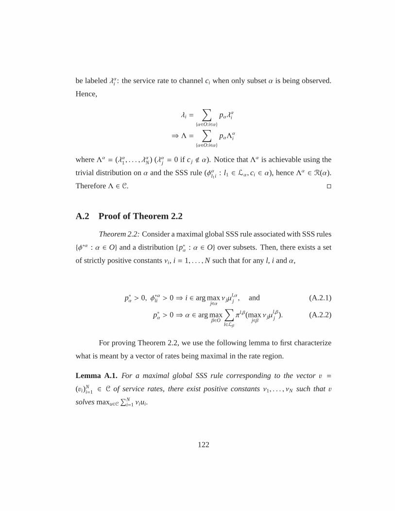
be labeledλαi : the service rate to channelci when only subsetα is being observed.

Hence,

λi =∑

α∈O:i∈αpαλ

αi

⇒ Λ =∑

α∈O:i∈αpαΛ

αi

whereΛα = (λα1, . . . , λαN) (λαj = 0 if cj < α). Notice thatΛα is achievable using the

trivial distribution onα and the SSS rule (φαl1i : l1 ∈ Lα, ci ∈ α), henceΛα ∈ R(α).

ThereforeΛ ∈ C.

A.2 Proof of Theorem 2.2

Theorem 2.2:Consider a maximal global SSS rule associated with SSS rules

φ∗α : α ∈ O and a distributionp∗α : α ∈ O over subsets. Then, there exists a set

of strictly positive constantsνi, i = 1, . . . ,N such that for anyl, i andα,

p∗α > 0, φ∗αli > 0⇒ i ∈ arg maxj∈α

ν jµl,αj , and (A.2.1)

p∗α > 0⇒ α ∈ arg maxβ∈O

∑

l∈Lβ

πl,β(maxj∈β

ν jµl,βj ). (A.2.2)

For proving Theorem 2.2, we use the following lemma to first characterize

what is meant by a vector of rates being maximal in the rate region.

Lemma A.1. For a maximal global SSS rule corresponding to the vectorv =

(vi)Ni=1 ∈ C of service rates, there exist positive constantsν1, . . . , νN such thatv

solvesmaxu∈C∑N

i=1 νiui.

122

Remark:The proof of the lemma is an application of the Arrow-Barankin-

Blackwell theorem [5]. For the sake of clarity, however, we give the full proof

here.

Proof. Let e1, . . . ,eM be all the extreme points ofC, with v =∑M

j=1 pjej and∑M

j=1 pj = 1, pj ≥ 0 j = 1, . . . ,M. Consider the following linear program:

maxζ,q j

ζ

subject to

M∑

j=1

qjeji ≥ ζvi , ∀i = 1, . . . ,N, (A.2.3)

M∑

j=1

qj = 1, 0 ≤ qj ≤ 1, ∀ j = 1, . . . ,M.

where eji denotes thei-th coordinate ofej. We know thatζ = 1 and

qj = pj solve this linear program with constraints (A.2.3) satisfied as equalities.

Then, by the Kuhn-Tucker theorem [34], there exists a set of non-negative Lagrange

multipliersν0, . . . , νN such thatζ = 1 andqj = pj also solve the following linear

program (with the same value of the maximum):

maxζ,q j

ν0ζ +

N∑

i=1

νi

M∑

j=1

qjeji − ζvi

(A.2.4)

subject to

M∑

j=1

qj = 1, 0 ≤ qj ≤ 1, ∀ j = 1, . . . ,M.

We note that everyνi must be strictly positive owing to the tightness in

(A.2.3), andν0 = 1. Rewriting (A.2.4), we get thatqj = pj maximizes

123

N∑

i=1

αi

M∑

j=1

qjeji

over all distributionsqj, i.e., v = (vi)Ni=1 maximizes

∑Ni=1 νiui over all u ∈

C.

Proof of Theorem 2.2.Let v∗ be the vector of long-term service rates for a maximal

global SSS rule parameterized by the distributionsφ∗α : α ∈ O andp∗α : α ∈ O.We have by Lemma A.1 that there exist positive constantsν1, . . . , νN such thatv∗

solves

maxv∈C

N∑

i=1

νivi

= maxpν,φν

N∑

i=1

νi

∑

ν

pν∑

l∈Lν

πl,νµl,νi φ

νli

= maxpν,φν

∑

ν

pν∑

l∈Lν

πl,νN∑

i=1

νiµl,νi φ

νli . (A.2.5)

Equivalently,pα = p∗α and φα = φ∗α solves (A.2.5), and properties

(A.2.1) and (A.2.2) of the theorem follow, since otherwise the maximum in (A.2.5)

would not be attained.

A.3 Proof of Lemma 2.4

Lemma 2.4:Let E be the (finite) set of extreme points for the achievable

rate regionC. If subsetδ is chosen inStep 1of Algorithm 1 at timet, then

R(δ) ∩ arg maxv∈E〈v,Q(t)〉 , ∅.

124

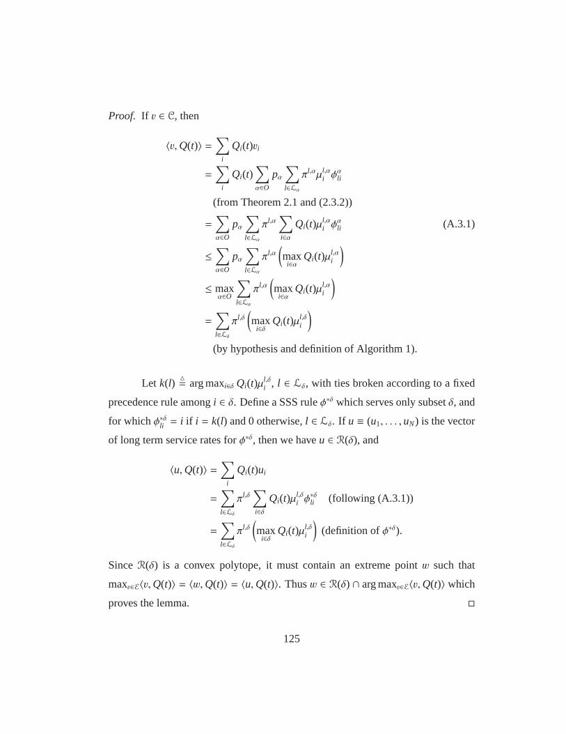
Proof. If v ∈ C, then

〈v,Q(t)〉 =∑

i

Qi(t)vi

=∑

i

Qi(t)∑

α∈Opα

∑

l∈Lα

πl,αµl,αi φ

αli

(from Theorem 2.1 and (2.3.2))

=∑

α∈Opα

∑

l∈Lα

πl,α∑

i∈αQi(t)µ

l,αi φ

αli (A.3.1)

≤∑

α∈Opα

∑

l∈Lα

πl,α(

maxi∈α

Qi(t)µl,αi

)

≤ maxα∈O

∑

l∈Lα

πl,α(

maxi∈α

Qi(t)µl,αi

)

=∑

l∈Lδ

πl,δ(

maxi∈δ

Qi(t)µl,δi

)

(by hypothesis and definition of Algorithm 1).

Let k(l)= arg maxi∈δ Qi(t)µ

l,δi , l ∈ Lδ, with ties broken according to a fixed

precedence rule amongi ∈ δ. Define a SSS ruleφ∗δ which serves only subsetδ, and

for whichφ∗δli = i if i = k(l) and 0 otherwise,l ∈ Lδ. If u ≡ (u1, . . . ,uN) is the vector

of long term service rates forφ∗δ, then we haveu ∈ R(δ), and

〈u,Q(t)〉 =∑

i

Qi(t)ui

=∑

l∈Lδ

πl,δ∑

i∈δQi(t)µ

l,δi φ∗δli (following (A.3.1))

=∑

l∈Lδ

πl,δ(

maxi∈δ

Qi(t)µl,δi

)

(definition ofφ∗δ).

SinceR(δ) is a convex polytope, it must contain an extreme pointw such that

maxv∈E〈v,Q(t)〉 = 〈w,Q(t)〉 = 〈u,Q(t)〉. Thusw ∈ R(δ) ∩ arg maxv∈E〈v,Q(t)〉 which

proves the lemma.

125

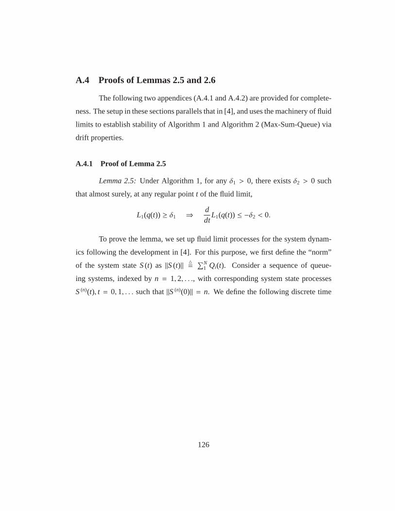
A.4 Proofs of Lemmas 2.5 and 2.6

The following two appendices (A.4.1 and A.4.2) are providedfor complete-

ness. The setup in these sections parallels that in [4], and uses the machinery of fluid

limits to establish stability of Algorithm 1 and Algorithm 2(Max-Sum-Queue) via

drift properties.

A.4.1 Proof of Lemma 2.5

Lemma 2.5:Under Algorithm 1, for anyδ1 > 0, there existsδ2 > 0 such

that almost surely, at any regular pointt of the fluid limit,

L1(q(t)) ≥ δ1 ⇒ ddt

L1(q(t)) ≤ −δ2 < 0.

To prove the lemma, we set up fluid limit processes for the system dynam-

ics following the development in [4]. For this purpose, we first define the “norm”

of the system stateS(t) as ||S(t)|| = ∑N1 Qi(t). Consider a sequence of queue-

ing systems, indexed byn = 1,2, . . ., with corresponding system state processes

S(n)(t), t = 0,1, . . . such that||S(n)(0)|| = n. We define the following discrete time

126

random processes fort = 0,1, . . . :

F(n)i (t)

= # of packets to queuei that arrived by timet,

F(n)i (t)

= # of queuei’s packets that got served by timet,

C(n)α (t)

= # of time slots beforet when subsetα was

chosen for scheduling,

Gα,(n)l (t)

= # of time slots beforet when subsetα was

picked and its sub-state wasl,

Gα,(n)li

= # of time slots beforet when subsetα was

picked, its observed sub-state wasl and queuei

was scheduled for service.

As in [4], for a canonical discrete time processZ(n)(t), define its correspond-

ing scaled(by n in space and time) process in continuous time by

z(n)(t)=

1n

Z(n)(⌊nt⌋), t ≥ 0,

following which we get the scaled versions of our system processes:

f (n) = ( f (n)i (t), t ≥ −1, i = 1,2, . . . ,N),

f (n) = ( f (n)i (t), t ≥ 0, i = 1,2, . . . ,N),

c(n) = (c(n)α (t), t ≥ 0, α ∈ O),

g(n) = (gα,(n)l (t), t ≥ 0, l ∈ Lα, α ∈ O),

g(n) = (gα,(n)li (t), t ≥ 0, l ∈ Lα, α ∈ O, i = 1,2, . . . ,N),

q(n) = (q(n)i (t), t ≥ 0, i = 1,2, . . . ,N).

For the sake of completeness, we reproduce (with minor modifications) the

following lemma from [4], which establishes convergence ofthese scaled processes

127

to the correspondingfluid limit processes. These fluid limit processes have desir-

able properties like being absolutely continuous and thus differentiable almost ev-

erywhere, non-decreasing and time-conserving.

(Lemma 1 in [4]). The following statements hold with probability 1. For

any sequence of processesX(n), there exists a subsequenceX(k), k ⊆ n, such that for

eachi, 1 ≤ i ≤ N, α ∈ O andl ∈ Lα,

( f (k)i (t), t ≥ −1)⇒ ( fi(t), t ≥ −1)

( f (k)i (t), t ≥ 0)→ ( fi(t), t ≥ 0) u.o.c.

( f (k)i (t), t ≥ 0)→ ( fi(t), t ≥ 0) u.o.c.

(q(k)i (t), t ≥ 0)→ (qi(t), t ≥ 0) u.o.c.

(gα,(k)l (t), t ≥ 0)→ (gαl (t), t ≥ 0) u.o.c.

(gα,(k)li (t), t ≥ 0)→ (gαli (t), t ≥ 0) u.o.c.

(c(k)α (t), t ≥ 0)→ (cα(t), t ≥ 0) u.o.c.

where the functionsfi are non-negative, non-decreasing and right-continuous with

left limits (RCLL) in [−1,∞), the functionsfi, fi, gαl , gαli , cα are non-negative non-

decreasing Lipschitz-continuous in [0,∞), functionsqi are continuous in [0,∞),

“⇒” signifies convergence at continuity points of the limit, and “u.o.c.” means

uniform convergence on compact sets, ask→ ∞. The limiting set of functions

x = ( f , f , g, g,q, c)

128

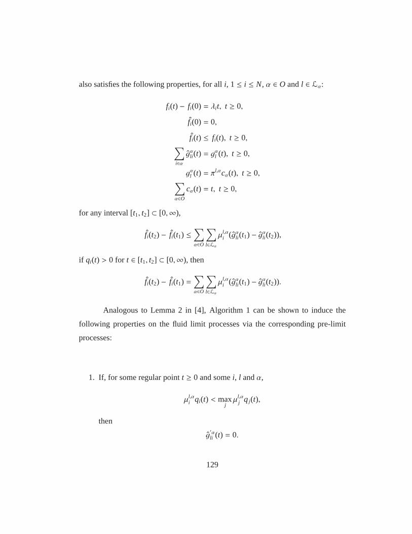
also satisfies the following properties, for alli, 1 ≤ i ≤ N, α ∈ O andl ∈ Lα:

fi(t) − fi(0) = λit, t ≥ 0,

fi(0) = 0,

fi(t) ≤ fi(t), t ≥ 0,∑

i∈αgαli (t) = g

αl (t), t ≥ 0,

gαl (t) = πl,αcα(t), t ≥ 0,∑

α∈Ocα(t) = t, t ≥ 0,

for any interval [t1, t2] ⊂ [0,∞),

fi(t2) − fi(t1) ≤∑

α∈O

∑

l∈Lα

µl,αi (gαli (t1) − gαli (t2)),

if qi(t) > 0 for t ∈ [t1, t2] ⊂ [0,∞), then

fi(t2) − fi(t1) =∑

α∈O

∑

l∈Lα

µl,αi (gαli (t1) − gαli (t2)).

Analogous to Lemma 2 in [4], Algorithm 1 can be shown to inducethe

following properties on the fluid limit processes via the corresponding pre-limit

processes:

1. If, for some regular pointt ≥ 0 and somei, l andα,

µl,αi qi(t) < max

jµl,α

j qj(t),

then

g′αli (t) = 0.

129

2. If, for some regular pointt ≥ 0 and someη,∑

l∈Lη

πl,η

(

maxi∈η

qi(t)µl,ηi

)

< maxα∈O

∑

l∈Lα

πl,α(

maxi∈α

qi(t)µl,αi

)

,

then

c′η(t) = 0.

Proof of Lemma 2.5.Since the system is assumed to be feasible, its rate vector isa

convex combination of feasible rate vectors of its maximal observable subsets, by

Lemma 2.3. Hence there must exist a fixed distributionpαα∈O together with subset

SSS rulesφαα∈O such that, using Theorem 1 of [4] and (A.1.1), we have

λi < vi(pα, φα) :=∑

α∈Opα

∑

l∈Lα

πl,αµl,αi φ

αli .

For any regulart ≥ 0 such thatL1(q(t)) > 0, the derivative ofL1(q(t)) can be

written as follows:

ddt

L1(q(t)) =N∑

i=1

qi(t)(λi − f ′i (t))

=

N∑

i=1

qi(t)(λi − vi(pα, φα)) + K(pα, φα,q(t))

− K(c′α(t), φα,q(t)), (A.4.1)

where we use the notation

K(rα, ψα, y) ≡∑

i

yi

∑

α

rα∑

l∈Lα

πl,αµl,αi ψ

αli ,

φαli ≡g′αli (t)

πl,αc′α(t),

and we use the fact, following from properties of the fluid limits, that

f ′i (t) =∑

α∈O

∑

l∈Lα

µl,αi g

′αli (t).

130

We can always chooseδ3 > 0 such thatL1(y) ≥ δ1 implies maxi yi ≥ δ3.

Then the first sum in (A.4.1) is bounded as follows:

N∑

i=1

qi(t)(λi − vi(pα, φα))

≤ −δ3 mini

(vi(pα, φα) − λi) ≡ −δ2.

It remains to show that

K(pα, φα,q(t)) ≤ K(c′α(t), φα,q(t)). (A.4.2)

Using Properties 1 & 2 of the fluid limit processes under Algorithm 1, we

have

K(c′α(t), φα,q(t))

=∑

i

qi(t)∑

α

c′α(t)∑

l∈Lα

πl,αµl,αi φ

αli

=∑

α

c′α(t)∑

l∈Lα

πl,α∑

i

qi(t)µl,αi φ

αli

= maxα

∑

l∈Lα

πl,α(

maxi

qi(t)µl,αi

)

= maxα

∑

l∈Lα

πl,α∑

i

qi(t)µl,αi φ

αli

≥∑

α

pα∑

l∈Lα

πl,α(

maxi

qi(t)µl,αi

)

≥∑

α

pα∑

l∈Lα

πl,α∑

i

qi(t)µl,αi φ

αli

= K(pα, φα,q(t)).

This proves Lemma 2.5.

131

A.4.2 Proof of Lemma 2.6

Lemma 2.6:Under Max-Sum-Queue scheduling, for anyδ1 > 0, there exists

δ2 > 0 such that almost surely, at any regular pointt of a fluid limit,

L2(q(t)) ≥ δ1 ⇒ ddt

L2(q(t)) ≤ −δ2.

To prove Lemma 2.6, we use the same framework of fluid limits asbefore

(Section A.4.1), this time working with a new Lyapunov function L2(·) where

L2(y)= max

β∈Ohβ(y),

and

hβ(y)=

12

∑

i∈βy2

i .

The following properties of the fluid limits under Max-Sum-Queue schedul-

ing follow from the properties of the pre-limit processes, in a manner similar to

Lemma 2 in [4]:

1. If, for some regular pointt ≥ 0 and somei, l andα,

µl.αi qi(t) < max

jµl,α

j qj(t),

then

g′αli (t) = 0.

2. If, for some regular pointt ≥ 0 and someη,

hη(q(t)) < maxα∈O

hα(q(t)),

then

c′η(t) = 0.

132

Proof of Lemma 2.6.Let arg maxα∈O hα(q(t)) be comprised ofβ1, . . . , βm with each

βi ∈ O, whereβ1 is chosen by a fixed precedence rule among subsets inO; thus

L2(q(t)) = 12

∑

i∈β1q2

i (t). For a regular pointt ∈ [0,∞), we have

ddt

L2(q(t)) =ddt

hβ1(t) =∑

i∈β1

qi(t)(λi − f ′i (t)) (A.4.3)

=∑

i∈β1

qi(t)

λi −

∑

l∈Lβ1

µl,β1i g

′αli (t)

=∑

i∈β1

qi(t)λi − c′β1(t)

∑

l∈Lβ1

πl,β1

∑

i∈β1

qi(t)µl,β1i φ

β1

li

=∑

i∈β1

qi(t)λi − c′β1(t)

∑

l∈Lβ1

πl,β1(maxi

qi(t)µl,β1i )

=∑

i∈β1

qi(t)λi − c′β1(t)Kβ1(q(t))

= 〈q(t), λ〉β1 − c′β1(t)Kβ1(q(t)) = w, say. (A.4.4)

whereφαli=

g′αli (t)

πl,αc′α(t) , Kα(y)=

∑

l∈Lαπl,α

(

maxi∈α yiµl,αi

)

for α ∈ O, 〈x, y〉α=

∑

i∈α xiyi,

and∑m

j=1 c′β j(t) = 1. More generally, as a result of the above, we have

ddt

hβ j (t) = 〈q(t), λ〉β j − c′β j(t)Kβ j (q(t))

∀ j = 1, . . . ,m. (A.4.5)

Sincet is a regular point, we have, using (A.4.5),

ddt

hβ j (q(t)) =ddt

hβ1(q(t)), ∀ j = 1, . . . ,m

⇒ 〈q(t), λ〉β j − c′β j(t)Kβ j (q(t))

= 〈q(t), λ〉β1 − c′β1(t)Kβ1(q(t)) ∀ j = 1, . . . ,m.

Define

qi(t)=

qi(t)Kβ j (q(t))

if i ∈ β j for somej, and 0 otherwise,

133

and letq(t)= (q1(t), . . . , qN(t)). q(t) is well-defined since a queuei belongs to at

most one of the (disjoint)β j. Consider

〈q(t), f ′(t)〉 =m∑

j=1

〈q(t), f ′(t)〉β j

=

m∑

j=1

∑

i∈β j

qi(t) f ′i (t)

=

m∑

j=1

[Kβ j (q(t))]−1∑

i∈β j

qi(t) f ′i (t)

=

m∑

j=1

[Kβ j (q(t))]−1c′β j(t)Kβ j (q(t))

(using (A.4.3)-(A.4.4))

=

m∑

j=1

c′β j(t) = 1.

Note that due to Step 2 of the Max-Sum-Queue policy,f ′(t)|β j maximizes

〈q(t), x〉β j over all x ∈ C. Hence by the above we have thatf ′(t) maximizes

〈q(t), x〉∪ jβ j over all x ∈ C. Sinceλ lies in the interior ofC, there existsǫ > 0

134

such that

〈q(t), λ〉 − 〈q(t), f (t)〉 ≤ −ǫ.

⇒ 〈q(t), λ〉 −m∑

j=1

c′β j(t) ≤ −ǫ

⇒m∑

j=1

〈q(t), λ〉β j −m∑

j=1

c′β j(t) ≤ −ǫ

⇒m∑

j=1

〈q(t), λ〉β j

Kβ j (q(t))−

m∑

j=1

c′β j(t) ≤ −ǫ

⇒m∑

j=1

〈q(t), λ〉β j − c′β j(t)Kβ j (q(t))

Kβ j (q(t))

≤ −ǫ

⇒ w

m∑

j=1

K−1β j

(q(t)) ≤ −ǫ.

∴ w ≤ −ǫ

m∑

j=1

K−1β j

(q(t))

−1

=: −δ2

wheneverL2(q(t)) ≥ δ1, since[∑m

j=1 K−1β j

(q(t))]−1

is monotone increasing inq(t).

This establishes the strictly negative drift and concludesthe proof.

A.5 Proof of Theorem 2.5

Theorem 2.5:Consider a symmetric system, where the observable subsets

are all subsets of a fixed cardinalityK. For such a system, Max-Sum-Queue is

throughput-optimal.

Proof. We show that Max-Sum-Queue is equivalent to the throughput-optimal rule

defined in Section 4 for a symmetric system. The throughput-optimal algorithm

135

picks a subsetγ ∈ O such that

γ ∈ arg maxα∈O

∑

ł∈Lα

πl,α(

maxi∈α

Qi(t)µl,αi

)

, (A.5.1)

while Max-Sum-Queue picks a subsetδ ∈ O such that

δ ∈ arg maxα∈O

∑

i∈αQ2

i (t)

i.e. δ contains the topK queues at timet. We claim thatδ belongs to the set in the

right hand side of (A.5.1). For if not, there exists a subsetη , δ such thatη does

not contain the topK queues and

∑

ł∈Lη

πl,η

(

maxi∈η

Qi(t)µl,ηi

)

>∑

ł∈Lδ

πl,δ

(

maxj∈δ

Q j(t)µl,δj

)

Assume without loss of generality that the queuesQii∈η andQ j j∈δ are ordered in

descending order within subsetsη andδ respectively. Since the system is symmet-

ric, each subset sees identical sub-states with identical distributions on them, so we

can assume thatLη andLδ are also identical, along with the corresponding sets of

πl,η andπl,δ. Hence we have

∑

ł∈Lη

πl,η

[(

maxi∈η

Qi(t)µl,ηi

)

−(

maxj∈δ

Q j(t)µl,δj

)]

> 0

which is a contradiction as each queue inδ is at least as large as its corresponding

queue inη. This proves the theorem.

A.6 Proof of Theorem 2.6

Theorem 2.6:The three-channel system considered in Section 2.6 is unsta-

ble under the Max-Sum-Queue scheduling policy. Furthermore, the Markov chain

136

describing the evolution of its state is transient.

We will need technical preliminaries similar to [84] to prove Theorem 2.6.

As stated earlier, fix the vector of arrival rates to beλ = (87,87,0.01). For each

n we split the nonnegative real line [0,∞) into equal contiguous intervals of size

nT each. Let thek-th interval [(k − 1)nT, knT) be denoted byCk. We divide every

interval uniformly intoPnT= nT/n1/4 equal contiguous sub-intervals of sizen1/4.

Define:

• Ai,n,kj : Number of arrivals from flowj in the i-th sub-interval of thek-th inter-

val, i.e. in [(k− 1)nT + (i − 1)n1/4, (k− 1)nT + in1/4), and

• Bi,n,km : Number of time slots that the channel is in statem in the i-th sub-

interval of thek-th interval, i.e. in [(k− 1)nT + (i − 1)n1/4, (k− 1)nT + in1/4).

We define the following arrival process and channel process deviation events:

En,kj (T, ν) =

⋃

1≤i≤PnT

∣∣∣∣∣∣∣

Ai,n,kj

n14

− λ j

∣∣∣∣∣∣∣

> ν

,

Gn,km (T, ν) =

⋃

1≤i≤PnT

∣∣∣∣∣∣

Bi,n,km

n14

− πm

∣∣∣∣∣∣> ν

.

Note that by hypothesis, the eventsEn,kj (T, ν) andGn,k

m (T, ν) are independent

for anyn, m, j, k, T > 0 andν > 0. For positive integersn andk and real numbers

T > 0 andν > 0 we define the following error event, corresponding to at least one of

the channel service rates or input flows being ‘atypical’ in its empirical distribution

in thek-th time interval:

137

Fn,k(T, ν) =

⋃

j

En,kj (T, ν)

⋃

⋃

m

Gn,km (T, ν)

.

The following lemma bounds from above the probability of this error event:

Lemma A.2. Fix T > 0, ν > 0 and ǫ > 0. Then, there exists n0 = n0(T, ν, ǫ) >

0 such that for all n> n0, for any fixed positive integer k, and uniformly over

a1, . . . ,a(k−1)nT−1, we have

P(

Fn,k(T, ν)∣∣∣A(1) = a1, . . . ,A((k− 1)nT − 1)

= a(k−1)nT−1) < ǫ.

Proof. Since by hypothesis there are only finitely many channels andaggregate

channel states, it suffices to show that

P(

En,kj (T, ν)

∣∣∣A(1) = a1, . . . ,A((k− 1)nT − 1)

= a(k−1)nT−1) < ǫ, (A.6.1)

and

P(

Gn,km (T, ν)

∣∣∣A(1) = a1, . . . ,A((k− 1)nT − 1)

= a(k−1)nT−1) < ǫ, (A.6.2)

for all k, j andm, andn large enough.

By Theorem 3.1.2 in [23], sinceAi is a finite-state irreducible discrete-time

Markov chain for everyi, the empirical meanAi,n,kj /n

14 obeys a large deviations

principle with a convex, good rate function. This means thatAi,n,kj /n

14 → λ j in

probability for everyj at a uniformly exponential rate. There are only a polynomial

138

(Tn34 ) number of sub-intervals in every interval of sizenT, hence (A.6.1) follows.

(A.6.2) is obtained in a similar manner since by Cramer’s Theorem [23], the empir-

ical mean ofiid random variables obeys a large deviations principle with a convex,

good rate function.

The lemma basically lets us assume that the empirical measures of the chan-

nel service rate and arrival processes look like their true measures, with very high

probability.

Let QS(k, t) denote the smallest queue length in the three queue lengths

Qi(k, t), i = 1,2,3, at the beginning of thet-th sub-interval in thek-th interval of

time. The following lemma is crucial to the proof of instability and describes how

the queueing system behaves in a typical interval.

Lemma A.3. Fix T > 0. There exists n1 ∈ Z+, ν > 0 and r > 0 such that for

any k ∈ Z+ and n > n1, conditioned on the fact that the event Fn,k(T, ν) has not

occurred, the following happens. If

minQ1(k, l),Q2(k, l),Q3(k, l) > n

for some l∈ 1, . . . ,PnT, then

QS(k, l + l′) − QS(k, l)l′

≥ r ∀ l′ ∈ 1. . . . ,PnT − l.

This lemma essentially tells us that in any typical interval, the lowest of

the three queues strictly increases with a uniform minimum rate, provided that the

queues are sufficiently large to start with.

139

Proof. Recall that a sub-interval consists ofn14 time slots. We can chooseν > 0 to

be much smaller than all theλi. If we denote by∆ (< ∞) the maximum possible

channel service rate in the system and byΛ the maximum of the three arrival rates

λ1, λ2, λ3, the change in any queue within an interval is at mostΓn14 whereΓ =

|Λ + ν − ∆|. We can pickδ > 0 sufficiently small, andn ∈ Z+ sufficiently large such

that this quantity is negligible compared to a queue length error of δn and such that

the second step of the Max-Sum-Queue policy is immune to queue length errors of

uptoδn if all queues are at least of lengthn.

Let Sδn(k, l) denote the subset of queues whose lengths are withinδn of the

smallest queue lengthQL(k, l), at the beginning of thel-th sub-interval in thek-th

interval. Without loss of generality we can assume thatSδn(k, ·) does not change

from l to l′, since if otherwise we can partition the set of intervals from l to l′ into

contiguous subsets with this property and obtain the resultusing the uniform bound

r.

The proof proceeds by considering various cases for the number of queues

in Sδn(k, l):

Case 1- Sδn(k, l) contains exactly one element: In this case, the single el-

ement is the unique smallest queue in the system, and remainsthe unique small-

est queue throughout, until sub-intervall′. Hence the only subset picked by the

first step of the Max-Sum-Queue policy is that consisting of the other two queues.

Consequently this queue is never served at all, and must increase at a rate at least

(minλ1, λ2, λ3 − ν) > 0.

Case 2- Sδn(k, l) contains exactly two elements: Here we need to consider

three further sub-cases:

2(a) - Sδn(k, l) = 1,2: In such a situation only the subset2,3 or 1,3can be picked by the first step of Max-Sum-Queue. Let us bound from above the

140

maximum rate at whichQ1 andQ2 together are served. If we assume (in the best

case) thatQ3 is never picked for service in the second step of Max-Sum-Queue,

thenQ1 andQ2 share the service time, and the total service rate to them is at most

200(12 + ν) + 150(12 − ν) = 150+ 50ν. The service discipline reduces to serving the

longest ofQ1 andQ2.

We claim that in this time, the difference|Q1−Q2| cannot exceed a constant

amount, say 10Γ, since if it did, then there was a last previous time when the order

of the queues was the same and the difference was under 5Γ. This implies that the

difference grew under the longest-queue policy, a contradiction.

The total arrival rate toQ1 andQ2, however, is at least 2(87− ν) = 174−2ν,

henceQ1+Q2 increases with a net rate of at least (174−2ν)−(150+50ν) = 24−52ν.

Hence their average increases with a net rate of at least (24− 52ν)/2 = 12− 26ν,

and sinceQ1 and Q2 remain within 10Γ of each other throughout andn can be

chosen large enough, the lowest queue increases with rate atleast (arbitrarily close

to) 12− 26ν > 0 for small enoughν > 0.

2(b) - Sδn(k, l) = 1,3: Here, the only possible subsets which can be picked

are1,2 and2,3. Note thatQ3 can never be served when the first subset is picked.

If the second subset is picked, sinceQ2 > Q1 always, the only state in whichQ1 is

served is when its rate is 200 andQ2’s rate is 100. HenceQ3 increases with a rate

at least 0.01− ν, while Q1 increases with a rate at least (87− ν) − (14 + ν)200 =

37− 201ν > 0 for small enoughν > 0.

2(c) - Sδn(k, l) = 2,3: Similar to the previous case by symmetry.

Case 3- Sδn(k, l) contains exactly three elements: In this case, all three

subsets are capable of being chosen in the first scheduling step.Q3 is never served,

hence its length increases at rate at least 0.01 − ν > 0. Partition the total time

141

into sections where(i) Q3 is the smallest queue,(ii) Q3 is between the other two

queues, and(iii) Q 3 is the largest queue. For(i), the smallest queueQ3 clearly

increases with rate bounded away from zero. For(ii) , only the subset consisting of

the top two queues is picked, hence the smallest queue increases with rate at least

87− ν > 0. For(iii) , we can use the same argument as with case2(a) to see that the

smallest queue increases with a strictly positive rate. This completes the proof.

Proof of Theorem 2.6.Fix anyT > 0. Lemma A.3 gives usn1, ν > 0 andr > 0 such

that in a typical interval (where the interval size isnT sub-intervals withn > n1),

if all queues are greater thann, then the lowest queue always increases with a rate

at leastr. Let R > 0 be the maximum possible service rate in the system (in this

caseR = 200), and letK = ⌈Rr ⌉ + 1 where⌈x⌉ denotes the smallest integer at least

x. Chooseǫ ∈ (0,1) small enough so thatǫ2K < 1, and furthermore, so that

(K − 1)ǫ2K

(1− ǫ2K)2+

2ǫ2K

1− ǫ2K< 1. (A.6.3)

Lemma A.2 now gives usn0 such that forn > n0 and anyk,

P(

Fn,k(T, ν)∣∣∣A(1) = a1, . . . ,A((k− 1)nT − 1) (A.6.4)

= a(k−1)nT−1) < ǫ, (A.6.5)

uniformly over alla1, . . . ,a(k−1)nT−1. Fix n to be any integer greater thann0 andn1.

Using the notationQS(k, t) introduced earlier to mean the length of the

smallest queue at the beginning of thet-th time sub-interval in thek-th time interval,

let X = (Xs : s= 1,2,3, . . .) be the random process denoting the size of the smallest

queue at the beginning of every interval of time:Xs = QS(s,1) ∀s = 1,2,3, . . .

Let m be an integer such thatm > n and let all queues start with initial statem:

Q1(1,1) = Q2(1,1) = Q3(1,1) = m.

142

Define the (time-valued) random variableτm to be the first time after starting

that X drops belowm: τm= mins > 1 : Xs ≤ m. We show thatP(τm < ∞) < 1,

implying that the smallest queue (and hence every queue) grows without bound with

a nonzero probability and establishing transience of the Markov chain describing

the evolution of the system stateS(t). We can write

P(τm < ∞) =∞∑

l=0

P(lK ≤ τm < (l + 1)K). (A.6.6)

Let Bl be the random variable which counts the number of atypical intervals

of time upto intervallK :

Bl=

lK∑

s=1

χFn,s(T,ν).

We claim thatlK ≤ τm < (l + 1)K implies Bl+1 ≥ l, for otherwiseBl+1 < l,

and by Lemma A.3, forlK ≤ t < (l + 1)K, we have

Xt ≥ m+ [t − Bl+1]rnT − Bl+1RnT

≥ m+ [lK − Bl+1]rnT − Bl+1RnT

= m+ nT[lKr − Bl+1(r + R)]

> m+ lnT[(K − 1)r − R]

≥ m,

a contradiction tolK ≤ τm < (l + 1)K.

143

From (A.6.6), we can write

P(τm < ∞) ≤∞∑

l=1

P(Bl ≥ l − 1)

=

∞∑

l=1

lK∑

l′=l−1

P(Bl = l′)

(a)≤

∞∑

l=1

lK∑

l′=l−1

(

lKl′

)

ǫ l′

≤∞∑

l=1

lK∑

l′=l−1

2lKǫ l

=

∞∑

l=1

((K − 1)l + 2)(ǫ2K)l

= (K − 1)∞∑

l=1

l(ǫ2K)l + 2∞∑

l=1

(ǫ2K)l

=(K − 1)ǫ2K

(1− ǫ2K)2+

2ǫ2K

1− ǫ2K

(b)< 1.

Here (a) is by applying (A.6.4) to

P(Bl = l′) = P

lK∑

s=1

χFn,s(T,ν) = l′

=∑

1≤i1<···<i l′≤lK

P(

χFn,i1(T,ν) = 1, . . . , χFn,il′ (T,ν) = 1,

χFn,i (T,ν) = 0, i < i1, . . . , i l′)

≤∑

1≤i1<···<i l′≤lK

ǫ l′

=

(

lKl′

)

ǫ l′ ,

and (b) follows from (A.6.3). This completes the proof.

144

Appendix B

Proofs for Chapter 3

B.1 Proof of Proposition 3.1

Proof. In the nth system, consider the joint channel states for the firstnT time

slots, i.e.,(

R(n)(1), R(n)(k), . . . ,R(n)(nT))

, with eachR(n)(k) ∈ RN ⊂ RN. Since

our sampling/scheduling rule is deterministic, the exact time slots in1, . . . ,nTat which useri is sampled depend entirely on these joint channel states. Toavoid

heavy notation, we will suppress the superscript (n) as all quantities we deal with

refer to thenth queueing system. LetV = (V1, . . . ,VN) be the (random)sampled

trace for the system upto timenT. By this, we mean that eachVi is a vector with

elements fromR that represents all the successively observed/sampled rates for

useri, i.e. Vi =(

Ri(Ki1),Ri(Ki2), . . .)

where useri is chosen precisely at time slots

Ki1,Ki2, . . . In other words,Vi is the ordered row of channel state values sampled

by the scheduling policy, so the sum of the lengths of theVi is exactlynT. In

the sequel, we frequently identify eachVi bijectively with its corresponding partial

sums processWi ≡W(Vi).

We have the following lemma, due to the crucial fact thatfor any determin-

istic sampling rule, the sampled trace uniquely specifies atwhat times each user

was sampled and its sampled channel states at those instants. By a valid sampled

trace, we mean a (finite) sampled trace occurring with nonzero probability. For a

valid sampled tracew in the n-th system, letE(w) be the set of all extended (i.e.

padded upto timenT arbitrarily with values inR) combinations ofw, i.e. the set of

145

all (e1, . . . ,eN) where eachei is a size-nT vector withwi a prefix of it.

Lemma B.1. Let Xi j , i = 1, . . . ,N, j = 1,2, . . . ,nT be independent random vari-

ables with Xi j ∼ Ri(0) for all i and j. Let P(nT) be the probability measure induced

by (Xi j )i, j. If w is a valid trace in the n-th system, then for any nq0 ∈ (Z+)N,

Pn,Tq0

[W(n) = w] = P(nT) [E(w)] .

Proof. Let w = (w1, . . . , wN) with∑N

i=1 |wi | = nT, and letv = (v1, . . . , vN) be the

corresponding sampled trace forw, i.e., eachwi is the vector of partial sums for the

vectorvi. Associated tow andv are the time slotski1, ki2, . . . when useri is sampled,

for all i. Furthermore, a key fact is that all the time slotski1, ki2, . . . when useri

is sampled, for alli, are completely specified byv due to the sampling rule being

nonrandom.

Recall, from our notation, that the random variableS(k) records which user

is sampled at time slotk. We have

Pn,Tq0

[W(n) = w] = Pn,Tq0

[V(n) = v](a)= Pn,T

q0[V(n) = v,∀i S(ki1) = i,S(ki2) = i, . . .]

= Pn,Tq0

[∀i Ri(ki1) = vi1,Ri(ki2) = vi2, . . .]

(b)=

∏

i, j

Pn,Tq0

[

Ri(ki j ) = vi j

]

(c)= P(nT) [E(w)] ,

which completes the proof. Here, (a) is by using the key fact in the preceding

paragraph; (b) is because channel states are independent across time and the fact

that theki j i, jare all distinct and partition1,2, . . . ,nT; (c) is due to exchangeability

of the (independent across time) channel state process.

146

Proceeding with the proof of the proposition, for eachq0 ∈ Q, we have

Pn,Tq0

[

q(n) ∈ Γ]

≤ Pn,Tq0

[

w(n) ∈ Γ(n)]

,

whereΓ(n) is the set of all valid sampled tracesw(n) that, together with someq′0 ∈ Q,

result in queue length pathsq(n) ∈ Γ under the scheduling algorithm. For an arbitrary

integern, we can write

Pn,Tq0

[

w(n) ∈ Γ(n)]

=∑

w∈Γ(n)

Pn,Tq0

[

w(n) = w]

=∑

w∈Γ(n)

P(nT) [E(w)] (by Lemma B.1)

= P(nT)

⋃

w∈Γ(n)

E(w)

(unique prefixes⇒ disjointness)

≤ P(nT)

∞⋃

n′=n

E(

Γ(n′))

.

∴ − lim supn→∞

n−1 log supq0∈QP

n,Tq0

[

w(n) ∈ Γ(n)]

≥ − lim supn→∞

n−1 log P(nT)

∞⋃

n′=n

E(

Γ(n′))

≥ inf

∫ 0

−T

N∑

i=1

Λ∗i (wi(z))dz : w ∈∞⋃

n′=n

E(

Γ(n′))

(by Mogulskii’s theorem [23])

⇒ − lim supn→∞

n−1 log supq0∈QP

n,Tq0

[

w(n) ∈ Γ(n)]

≥ (B.1.1)

limn→∞

inf

∫ 0

−T

N∑

i=1

Λ∗i (wi(z))dz : w ∈∞⋃

n′=n

E(

Γ(n′))

. (B.1.2)

Let the right hand side of (B.1.2) be denoted byζ. For everyn = 1,2, . . ., we can

147

choosewn such that

wn ∈∞⋃

n′=n

E(

Γ(n′))

, and

limn→∞

∫ 0

−T

N∑

i=1

Λ∗i (wn,i(z))dz= ζ.

Since thewn are all uniformly Lipschitz continuous and bounded, by the Arzela-

Ascoli theorem, the sequence(wn)n contains a subsequence converging uniformly

over the time interval [−T,0]. Without loss of generality, let the subsequence be

n itself, and let limn→∞ wn = w. The map f 7→∫ 0

−T

∑Ni=1Λ

∗i ( f (z))dz is lower-

semicontinuous [23], thus

∫ 0

−T

N∑

i=1

Λ∗i (w(z))dz≤ limn→∞

∫ 0

−T

N∑

i=1

Λ∗i (wn,i(z))dz= ζ.

We can pick, for each ˆn, anmn and awmn ∈⋃∞

n′=n E(

Γ(n′))

such that||wmn − wn||∞ <1/n. Sincewmn ∈

⋃∞n′=n E

(

Γ(n′))

, let wmn ∈ E(

Γ(m′n))

for somem′n ≥ n. It follows

that there exists a corresponding valid queue length pathqmn such thatwmn induces

qmn, and moreover,qmn ∈ Γ. We can pick a subsequence ofmnn (let it be mn

without loss of generality) along whichqmn converges to aq ∈ Γ = Γ. We now have

lim n→∞ wmn = w and limn→∞ qmn = q, thus (q, w) is a valid fluid sample path with

q ∈ Γ andq(−T) ∈ Q. This yields

− lim supn→∞

n−1 log supq0∈QP

n,Tq0

[

w(n) ∈ Γ(n)]

≥

inf

∫ 0

−T

N∑

i=1

Λ∗i (wi(z))dz : (w,q) an FSP,q ∈ Γ,q(−T) ∈ Q

148

⇒ − lim supn→∞

1n

log supq0∈QP

n,Tq0

[

q(n) ∈ Γ]

≥

inf

∫ 0

−T

N∑

i=1

Λ∗i (wi(z))dz : (w,q) an FSP,q ∈ Γ,q(−T) ∈ Q

.

(B.1.3)

Note: By (w,q) being an FSP, in addition to there existing pre-limit se-

quencesw(n) → w andq(n) → q (uniformly over [-T,0]), we mean that there exist

pointszi ∈ [−T,0] for all i = 1, . . . ,N such thatz(n)i → ti asn→ ∞, wherez(n)

i is the

(scaled by 1/n) index in the sampled tracew(n)i beyond which useri is never sam-

pled (i.e. it is the last index at which useri is sampled by the scheduling algorithm

if user i’s samples are stacked successively and contiguously).

From the observation preceding Lemma B.1, each sampled tracew(n) com-

pletely specifies the exact instants at which each user was scheduled/sampled and

the channel states observed at those instants, i.e.w(n) completely specifies the pair

(m(n), c(n)) in [−T,0]. The next lemma relates the large deviations “costs” of the fluid

limits of sampled traces to those of the fluid limits of their associated (m(n), c(n)) pro-

cesses.

Lemma B.2. Let (w,q) be a fluid sample path withw(n) → w and q(n) → q. Let

(m(n), c(n)) be the scaled sampled rate and selection processes specifiedbyw(n) → w.

For every subsequential limit(m, c) of (m(n), c(n))n (in the || · ||∞ topology on[−T,0]),N∑

i=1

∫ zi

−TΛ∗i (wi(z))dz=

∫ 0

−T

N∑

i=1

ci(t)Λ∗i

(

mi(t)ci(t)

)

dt.

Proof. Assume without loss of generality thatm(n) → m andc(n) → c uniformly in

[−T,0]. Let−T ≤ t1 ≤ t2 ≤ 0. For alln, by the definition of the sampled tracesw(n)i ,

we have

w(n)i

(

c(n)i (t2)

)

− w(n)i

(

c(n)i (t1)

)

= m(n)i (t2) −m(n)

i (t1) +O(1/n). (B.1.4)

149

By the (uniform) convergence hypotheses, forj ∈ 1,2, c(n)i (t j) → ci(t j), thus

w(n)i

(

c(n)i (t j)

)

→ wi(ci(t j)). Lettingn→ ∞ in (B.1.4),

wi (ci(t2)) − wi (ci(t1)) = mi(t2) −mi(t1). (B.1.5)

Sinceci and mi are nondecreasing Lipschitz-continuous functions, they induces

Stieltjes measuresdci anddmi respectively on [−T,0] with dmi << dci. In a simi-

lar fashion,wi induces a Stieltjes measuredwi << dzon [−T, zi] wheredzdenotes

Lebesgue measure. Letdwi/dz be the Radon-Nikodym derivative ofdwi with re-

spect to Lebesgue measure, and consider∫ t2

t1

dwi

dz ci(t)dci(t) =

∫ ci (t2)

ci (t1)

dwi

dz(z)

(

dci c−1)

(change of variables formula)

=

∫ ci (t2)

ci (t1)

dwi

dz(z)dz (dci c−1 ≡ Lebesgue[−T, zi])

= wi (ci(t2)) − wi (ci(t1))

= mi(t2) −mi(t1) (thanks to (B.1.5))

=

∫ t2

t1

dmi(t)

⇒ dwi

dz ci(·) =

dmi

dci(·) dci-a.e. on [−T,0].

With this, we can finally compute∫ 0

−Tci(t)Λ

∗i

(

mi(t)ci(t)

)

=

∫ 0

−T

(

Λ∗ dmi

dci

)

(t)dci(t)

=

∫ 0

−T

(

Λ∗ dwi

dz ci

)

(t)dci(t) =∫ ci (0)

ci (−T)

(

Λ∗ dwi

dz

)

(z)(

dci c−1)

=

∫ zi

−T

(

Λ∗ dwi

dz

)

(z)dz=∫ zi

−TΛ∗ (wi(z)) dz.

This proves the lemma.

Applying the result of Lemma B.2 to (B.1.3) concludes the proofof Propo-

sition 3.1.

150

B.2 Proof of Proposition 3.3

Proof. Denote byC(φ′1, . . . , φ′N) the convex hull of the points (0, . . . ,0), (φ′1, . . . ,0),

(0, φ′2, . . . ,0), . . . , (0, . . . , φ′N). The right-hand side of (3.5.4) is trivially∞ if either

(a)λ ∈ C(φ′1, . . . , φ′N), or (b) any of theφ′i is not in the effective domain of its corre-

spondingΛ∗i ; we exclude suchφ′i andλ in the remainder of the proof.

For eachn = 1,2, . . ., let tn ≥ 0 be a nonrandom time, to be specified later

(to avoid complications, we assumentn is an integer). Consider

Pπ[

||q(n)(0)||∞ ≥ 1]

= Pπ[

||q(n)(tn)||∞ ≥ 1]

≥ Pπ[

||q(n)(tn)||∞ ≥ 1 | ||q(n)(0)||∞ = 0]

Pπ[

||q(n)(0)||∞ = 0]

= π((0,0, . . . ,0)) Pπ0[

||q(n)(tn)||∞ ≥ 1]

.

Here,π(·) is used to denote the stationary distribution that the policy π induces, and

Pπ0 represents the stationary distribution conditioned on thestarting state being the

origin (all zeroes).

The non-negativity of queues forces the relationU (n)(k)= λn − M(n)(k) ≤

Q(n)(k), whereU (n)(k) =∑k

l=1(λ − R(n)(l)δS(l)) represents the “unreflected queue

lengths” in then-th queueing system at timek. By suitably rescaling in time and

space, we can continue this chain of inequalities as

Pπ[

||q(n)(0)||∞ ≥ 1]

≥ π((0,0, . . . ,0)) Pπ0

[

maxi

u(n)i (tn) ≥ 1

]

. (B.2.1)

For eachi = 1, . . . ,N, sinceφ′i is in the effective domain of its Cramer rate function

Λ∗i , it follows that there existsη′i ∈ R such thatΛ∗i (φ′i ) = η

′iφ′i − Λi(η′i ). Define for

eachi an exponentially tilted measurePi (with respect to the marginal measurePi

of the i-th channel stateRi(0)) onR as follows:

Pi(dx)= exp[η′i x− Λi(η

′i )] Pi(dx) = exp[η′i (x− φ′i ) + Λ∗i (φ′i )] Pi(dx).

151

A standard computation under the tilted measure yieldsEi[Ri(0)] = φ′i . As with the

approach followed in [86], letPπ0 be the measure defined similarly toPπ0 except that

the twisted measuresPi replacePi as the conditional marginal distributions of

the sampled channel states/rates, withEi being the corresponding expectations.

Let us define

t−1min

= max

iλi ,

t−1max

= min

µ∈C(φ′1,...,φ′N)

maxi

(λi − µi).

Since by hypothesis the arrival rateλ is outside the closed setC(φ′1, . . . , φ′N), it fol-

lows that 0< tmin ≤ tmax < ∞. The timestmin and tmax represent the earliest and

latest time that the maximum queue length can take to overflowto level 1 in a sys-

tem of queues with “fluid” inputs at ratesλi that can be drained with instantaneous

rates in the convex hullC(φ′1, . . . , φ′N).

The remainder of the proof is organized into four steps:

1. Showing that forn large enough, under the twisted measureP, the service

m(n)i (t) provided to the queuei is approximated with high probability byφ′i ci(t),

i.e. we can treat the channel as being deterministic with a service rate ofφ′i ,

2. Under the conditions of the previous step, overflow of the unreflected max-

queued(n)(·) is inevitable by time roughlytmax, so with a significant proba-

bility the first hitting time ofd(n)(·) to level 1 is at mosttmax. Thus, we can

find a time not exceedingtmax at which overflow occurs with a significant

probability (i.e. not decaying to 0 exponentially inn)

152

3. Overflow occurring at the time in the previous step, under the conditions of

step 1, forces the scheduling “choice fractions”c(n)(t)/t to be “consistent”

with overflow ofd(n)(·) occurring at that time

4. Using all the steps to develop the right-hand side of (B.2.1) and derive the

stated result.

B.2.0.1 Step 1 of 4

Let us record the following definition. For eachi = 1, . . . ,N, we can write

m(n)i (t) ≡ mi(t) =

1n

Mi(nt) =1n

nt∑

l=0

Ri(l)Xi(l) =Mi(nt)

n+φ′in

nt∑

l=0

Xi(l)

=Mi(nt)

n+φ′in

Ci(nt),

= mi(t) + φ′i ci(t),

whereXi(l) is the indicator of the event that useri was scheduled at time slotl, and

Mi(k)=

∑kl=0(Ri(l)− φ′i )Xi(l) is the (unscaled) “centered” service provided to queue

i upto time slotk.

Lemma B.3. Let times t1 and t2, such that0 < t1 ≤ t2, andδ > 0 be fixed. Then,

limn→∞Pπ0

[

|m(n)i (t)| < δt ∀t ∈ [t1, t2]

]

= 1.

Proof. Observe that for eachi, Mi(k)k is a martingale (with respect to the measure

Pπ0) null at 0 and with differences bounded byD= (Rmax+maxi φ

′i ), whereRmax is

the maximum channel rate across all channels in the system. An application of the

Azuma-Hoeffding martingale inequality [59] thus gives

Pπ0

∣∣∣∣∣∣

Mi(k)k

∣∣∣∣∣∣≥ γ

≤ 2e−kγ2

2D2 (B.2.2)

153

for all k = 1,2, . . .. Hence, a union bound gives

1−Pπ0[|mi(t)| < δt ∀t ∈ [t1, t2]

]

= Pπ0[∃t ∈ [t1, t2] |mi(t)| ≥ δt

]

≤nt2∑

k=nt1

Pπ0

∣∣∣∣∣∣

Mi(k)k

∣∣∣∣∣∣≥ δ

≤nt2∑

k=nt1

2e−kδ2

2D2

≤ 2n(t2 − t1)e− nt1δ

2

2D2n→∞−→ 0 (∵ t1 > 0),

which is the stated result.

B.2.0.2 Step 2 of 4

Let us fixδ > 0 small enough, and letǫ > 0 be such that

(tmax+ ǫ)−1 = min

µ∈C(φ′1,...,φ′N)

maxi

(λi − δ − µi).

Additionally, fix a timet0 > 0 small enough, and letA ≡ An denote the event whose

(twisted) probability is estimated in Lemma B.3, i.e.

An ≡ An(δ) ≡ An(δ, t0, tmax)=

|m(n)i (t)| < δt ∀t ∈ [t0, tmax]

.

Denote the (unreflected and fluid-scaled) maximum queue length process

by d(·) ≡ d(n)(·) = maxi u(n)i (·). It follows that in the eventAn, d(·) must overflow

(i.e. hit level 1) at least once by time (tmax+ ǫ). In other words, if we let

τ ≡ τn= inf

t = 0,1n,2n, . . . : d(t) ≥ 1

,

thenAn ⊆ τn ≤ tmax+ ǫ. For eachn = 1,2, . . ., define the (deterministic)

time

tn= arg max

t=0, 1n ,...,tmax+ǫPπ0 [τn = t]

154

with ties broken in an arbitrary fashion. Observe thattn does not depend uponδ, t0

or An. Also, note that

Pπ0 [An] ≤ Pπ0 [τn ≤ tmax+ ǫ] ≤

∑

t=0, 1n ,...,tmax+ǫ

Pπ0 [τn = t]

≤ n(tmax+ ǫ)

maxt=0, 1n ,...,tmax+ǫ

Pπ0 [τn = t]

≤ n(tmax+ ǫ)Pπ0 [τn = tn]

⇒ Pπ0 [τn = tn] ≥

Pπ0 [An]

n(tmax+ ǫ)

Since the rate of change ofd(n)(·) is bounded byD, we can write

⇒ Pπ0[

d(tn) ∈[

1,1+Dn

]]

≥ Pπ0 [τn = tn] ≥Pπ0 [An]

n(tmax+ ǫ). (B.2.3)

B.2.0.3 Step 3 of 4

This step involves showing that when the queues overflow at time tn then

the scheduling choice fractionsc(n)(tn)/tn at that time are very likely to be the ones

that cause “straight-line” overflow at timetn from the all-empty queue state.

Recall thatδ > 0 is a sufficiently small number. We denote byΓn the set of

δ-compatiblescheduling fractions for overflow at timetn as follows:

Γn ≡ Γn(δ, tn)=

( f ′1, . . . , f ′N) :

∑

i

f ′i = 1, f ′i ≥ 0,maxi

(

λitn − φ′i f ′i tn) ∈ [1 − δtn,1+ δtn]

.

Lemma B.4. For all n large enough andδ > 0,

Pπ0

[

d(tn) ∈[

1− Dn,1+

Dn

]

,c(tn)tn< Γn

]

≤ 2Ne−nt0δ

2

8D2 .

Proof. Forn sufficiently large,

d(tn) ∈[

1− Dn,1+

Dn

]

⇒ d(tn) ∈[

1− δ2

tn,1+δ

2tn]

.

155

Also,

d(tn) ∈[

1− δ2

tn,1+δ

2tn]

,c(tn)tn< Γn⇒ ∃i |mi(tn)| >

δ

2tn.

Thus,

Pπ0

[

d(tn) ∈[

1− Dn,1+

Dn

]

,c(tn)tn< Γn

]

≤ Pπ0[

∃i |mi(tn)| >δ

2tn]

≤∑

i

Pπ0

[

|mi(tn)| >δ

2tn]

≤∑

i

2e−ntnδ2

8D2 (Azuma-Hoeffding (B.2.2))

≤ 2Ne−nt0δ

2

8D2 .

Step 4 of 4

We can now finally develop the right-hand side of (B.2.1) usingthe results

from the previous steps:

Pπ0

[

maxi

u(n)i (tn) ≥ 1

]

= Pπ0

[

d(n)(tn) ≥ 1]

≥ Pπ0[

d(n)(tn) ≥ 1, c(n)(tn)/tn ∈ Γn

]

= Eπ0[

1d(tn)≥1,c(tn)/tn∈Γn]

= Eπ0

1d(tn)≥1,c(tn)/tn∈Γn

ntn∏

l=0

exp[

−Λ∗U(l)(φ′U(l)) − η′U(l)

(

RU(l)(l) − φ′U(l)

)]

= Eπ0

1d(tn)≥1,c(tn)/tn∈Γn exp

−ntn

∑

i

ci(tn)tnΛ∗i (φ

′i )

exp[−nw(tn)]

with w(tn) ≡ w(n)(tn)=

1n

W(ntn)=

1n

ntn∑

l=0

η′U(l)

(

RU(l)(l) − φ′U(l)

)

= Eπ0

1d(tn)≥1,c(tn)/tn∈Γn exp

−ntn

supf ′∈Γn

∑

i

f ′i Λ∗i (φ′i )

exp[−nw(tn)]

= exp

−ntn

supf ′∈Γn

∑

i

f ′i Λ∗i (φ′i )

Eπ0

[

1d(tn)≥1,c(tn)/tn∈Γne−nw(tn)

]

. (B.2.4)

156

The second term in the product above can be bounded from belowfor anyζ > 0 as

follows:

Eπ0

[

1d(tn)≥1,c(tn)/tn∈Γne−nw(tn)

]

≥ Eπ0[

1d(tn)≥1,c(tn)/tn∈Γn,|w(tn)|<ζe−nζ

]

= e−nζPπ0

[

d(tn) ≥ 1,c(tn)tn∈ Γn, |w(tn)| < ζ

]

≥ e−nζPπ0

[

d(tn) ∈[

1,1+Dn

]

,c(tn)tn∈ Γn, |w(tn)| < ζ

]

. (B.2.5)

We have

Pπ0

[

d(tn) ∈[

1,1+Dn

]

,c(tn)tn∈ Γn, |w(tn)| < ζ

]

≥ Pπ0[

d(tn) ∈[

1,1+Dn

]

,c(tn)tn∈ Γn

]

− Pπ0[|w(tn)| ≥ ζ

]

≥ Pπ0[

d(tn) ∈[

1,1+Dn

]]

− Pπ0[

d(tn) ∈[

1,1+Dn

]

,c(tn)tn< Γn

]

− Pπ0[|w(tn)| ≥ ζ

]

.

(B.2.6)

By definition and the properties of the twisted distributionP, it can be seen that

W(k)k=0,1,... is again a martingale null at 0 and with bounded increments (bounded

by, say,D2= maxi η

′i (Rmax+ φ

′i )). Hence, the Azuma-Hoeffding inequality applied

to it yields

Pπ0

[|w(tn)| ≥ ζ] ≤ 2e

− nζ2

2tnD22 ≤ 2e

− nζ2

2tmaxD22 .

Using this and the results of Steps 2 and 3, (B.2.6) becomes

Pπ0

[

d(tn) ∈[

1,1+Dn

]

,c(tn)tn∈ Γn, |w(tn)| < ζ

]

≥Pπ0 [An]

n(tmax+ ǫ)− 2Ne−

nt0δ2

8D2 − 2e− nζ2

2tmaxD22

≥ 1/2n(tmax+ ǫ)

− 2Ne−nt0δ

2

8D2 − 2e− nζ2

2tmaxD22 (for n large enough, by Step 1).

157

The first term above decays asn−1 while the second and third terms decay exponen-

tially in n, thus

− lim infn→∞

1n

log Pπ0

[

d(tn) ∈[

1,1+Dn

]

,c(tn)tn∈ Γn, |w(tn)| < ζ

]

≤ 0. (B.2.7)

What remains is to bound the first term in the product in (B.2.4).By definition, for

every f ′ ∈ Γn, we have

maxi

(λi − φ′i f ′i ) ≤ 1tn+ δ

⇒ tn supf ′∈Γn

∑

i

f ′i Λ∗i (φ′i ) ≤ sup

f ′∈Γn

∑

i f ′i Λ∗i (φ′i )

maxi(λi − φ′i f ′i ) − δ

≤ sup∑

i f ′i =1f ′i ≥0

∑

i f ′i Λ∗i (φ′i )

maxi(λi − φ′i f ′i ) − δ. (B.2.8)

Applying the conclusions of (B.2.5), (B.2.7) and (B.2.8) to (B.2.4), we get

− lim infn→∞

1n

logPπ0

[

maxi

u(n)i (tn) ≥ 1

]

≤ ζ + sup∑

i f ′i =1f ′i ≥0

∑

i f ′i Λ∗i (φ′i )

maxi(λi − φ′i f ′i ) − δ.

The arbitrary choice ofζ > 0 andδ > 0 implies that

− lim infn→∞

1n

logPπ0

[

maxi

u(n)i (tn) ≥ 1

]

≤ sup∑

i f ′i =1f ′i ≥0

∑

i f ′i Λ∗i (φ′i )

maxi(λi − φ′i f ′i ).

The stationary distributionPπ induced by the (stabilizing) scheduling policyπ forces

π((0,0, . . . ,0)) > 0, so (B.2.1) finally implies

− lim infn→∞

1n

logPπ[

||q(n)(0)||∞ ≥ 1]

≤ sup∑

i f ′i =1f ′i ≥0

∑

i f ′i Λ∗i (φ′i )

maxi(λi − φ′i f ′i ),

completing the proof of the proposition.

158

B.3 Proof of Proposition 3.4

Proof. Recall thatJ∗ is the infimum

J∗= inf

T,(mT ,cT ,qT )0≤t≤T

∑Ni=1 ci(t)Λ∗i

(mi (t)ci (t)

)

ddt ||q(t)||∞

(B.3.1)

over all feasible Fluid Sample Paths at regular pointst. There is nothing to be done

if the right hand side above is∞, so we exclude this case. We have the following

characterization of regular points under the Max-Queue scheduling algorithm.

Lemma B.5. Under the Max-Queue policy, let s(t)= arg maxi=1,...,N qi(t) ⊆ 1, . . . ,N.

If t is a regular point, then

1. c′i (t) = 0 ∀i < s(t), i.e., the non-maximum fluid queues do not receive service,

2. ddt ||q(t)||∞ = λi −m′i (t) ∀i ∈ s(t), i.e., all the maximum fluid queues grow at the

same rate.

Thus, by Lemma B.5,

J∗ ≥ infS⊆1,...,N

∑

i∈S c′iΛ∗i

(

φ′i

)

w′, (B.3.2)

for all non-negativec′i i∈S, φ′i i∈S satisfying∑

i∈S c′i = 1, andw′ = λi − c′iφ′i ∀i ∈ S.

Note that the denominatorw′ is strictly positive if and only ifλ < C(φ′1, . . . , φ′N),

and that eachφ′i can be restricted to be at mostE[Ri] (since ifφ′i > E[Ri], reducing

φ′i to E[Ri] only gives a lesser fraction above).

For a subsetS ⊆ 1, . . . ,N, let

DS=

(φ′i )i∈S : Rmin,i ≤ φ′i ≤ E[Ri], ∃c′i ≥ 0 with∑

i∈Sc′i = 1, ∀i, j ∈ S,

λi − c′iφ′i = λ j − c′jφ

′j = w

′ > 0

.

159

It can be shown that for each such tupleφ′ ∈ DS, there is auniquecorresponding

tuplec′ and hence auniquew′ (this follows because the point (c′iφ′i )i∈S must be the

point where the diagonal fromφ′ pierces the convex hullC((φ′i )i∈S)). Thus, if we

define a mapf S : DS → R+ by

f S(φ′)=

∑

i∈S c′iΛ∗i

(

φ′i

)

w′, (B.3.3)

then (B.3.2) is just

J∗ ≥ minS

infφ′S∈DS

f S(φ′S). (B.3.4)

The next lemma contains the key result needed to prove Proposition 3.4:

Lemma B.6. Let S⊆ 1, . . . ,N be such thatDS , ∅. Then,

1. fS attains its infimum overDS at a pointφ′S ∈ DS.

2. Let c′ be the (unique) tuple corresponding toφ′S such that0 < λi − c′i φ′i =

λ j − c′jφ′j ∀i, j ∈ S . Then, for everyc′i i∈S with c′i ≥ 0,

∑

i∈S c′i = 1, we have

f S(φ′S) ≥∑

i∈S c′iΛ∗i (φ′i )

maxi∈S(λi − c′i φ′i ).

Proof. Without loss of generality, we will assumeS = 1, . . . ,N. Denoteµi=

E[Ri]. λ is a stabilizable vector of arrival rates, soλ ∈ C(µ1, . . . , µN) (hereµi is

overloaded to denote theN-tuple with thei-th coordinate beingµi and the remaining

coordinates being 0). Hence, there existsδ > 0 such that∑N

i=1λi

µi= 1− δ.

For anyφ′ ∈ DS, we have∑N

i=1λi

φ′i> 1 by definition. Thus,

∑Ni=1

λi

φ′i>

(1

1−δ

)∑Ni=1

λi

µi, so φ′j < (1 − δ)µ j for at least onej. It follows from the proper-

ties of the Cramer rate function for finite alphabets [23] that for eachi, Λ∗i (·) is

160

strictly decreasing on [Rmin,i , µi], with Λ∗i (µi) = 0. Denote byγ the positive number

mini Λ∗i ((1 − δ)µi). Fix ǫ > 0 small enough. If additionally (forφ′ ∈ DS) w′ < ǫ,

then

f S(φ′) =

∑

i c′iΛ∗i (φ′i )

w′≥

c′jΛ∗j (φ′j)

w′=

λ j − w′

φ′jw′

Λ∗j (φ′j) >

(λ j − ǫµ jǫ

)

γ.

This means that for everyB > 0, there existsǫB > 0 such thatφ′ ∈ DS : w′ < ǫB ⊆φ′ ∈ DS : f S(φ′) > B. Thus,

infφ′∈DS

f S(φ′) = infφ′∈DS:w′≥ǫB

f S(φ′).

Observe thatφ′ ∈ DS : w′ ≥ ǫB is a compact set, and that the lower-semicontinuity

of Λ∗i (·) [23] forces f S to be lower-semicontinuous on this compact set. It follows

that f S achieves its infimum on this set and thus onDS. This proves the first part of

the lemma.

Turning to the second part, letφ′S ∈ DS infimize f S(·) overDS, with Rmin,i ≤φ′i ≤ µi ∀i ∈ S. Fix any i ∈ S. Sinceφ′S is a minimizer, increasingφ′i = φ′i by a

small amount (keeping the other coordinates unchanged andφ′S within DS) cannot

decreasef S(φ′S), i.e., ∂∂φ′i

f S(φ′S)∣∣∣∣φ′S

≥ 0. From the definition off S (B.3.3), we can

write ∂∂φ′i

f S(φ′S) = ∂∂φ′i

ND , whereN ≡ N(φ′S) =

∑

i∈S c′iΛ∗i (φ′i ), andD ≡ D(φ′S) = w′ ≡

w′(φ′S). Thus,

0 ≤ ∂

∂φ′if S(φ′S)

∣∣∣∣∣∣φ′S

=1

D2(φ′S)

(

D(φ′S)∂

∂φ′iN(φ′S) − N(φ′S)

∂

∂φ′iD(φ′S)

)∣∣∣∣∣∣φ′S

. (B.3.5)

Define, for eachi, η′i=Λ∗i (φ′i )φ′i

(and η′i=Λ∗i (φ′i )

φ′i). Noticing that ∂

∂φ′iD(φ′S) = ∂

∂φ′i(λ j −

c′jφ′j) = −

∂∂φ′i

(c′jφ′j) for all j ∈ S, we can write

∂

∂φ′iN(φ′S) =

∂

∂φ′i

∑

j∈Sc′jφ′jη′j = −

∂D(φ′S)

∂φ′i·∑

j∈Sη′j + c′iφ

′i ·∂η′i∂φ′i

.

161

Along with (B.3.5), this implies (evaluated atφS = φ′S)

0 ≤ −D(φ′S) ·∂D(φ′S)

∂φ′i·∑

j∈Sη′j + D(φ′S) · c′iφ′i ·

∂η′i∂φ′i− N(φ′S)

∂D(φ′S)

∂φ′i

= −∂D(φ′S)

∂φ′i

D(φ′S) ·

∑

j∈Sη′j + N(φ′S)

+ D(φ′S) · c′iφ′i ·

∂η′i∂φ′i

= −∂D(φ′S)

∂φ′i

D(φ′S) ·

∑

j∈Sη′j + N(φ′S)

+ D(φ′S) · c′iφ′i ·

φ′i∂Λ∗i (φ′i )∂φ′i− Λ∗i (φ′i )

φ′2i

= −∂D(φ′S)

∂φ′i

D(φ′S) ·

∑

j∈Sη′j + N(φ′S)

− D(φ′S)c′iη

′i + D(φ′S) · c′i ·

∂Λ∗i (φ′i )

∂φ′i︸ ︷︷ ︸

≤0

≤ −∂D(φ′S)

∂φ′i︸ ︷︷ ︸

≤0

D(φ′S) ·

∑

j∈Sη′j + N(φ′S)

− D(φ′S)c′iη

′i

⇒ ND≥ −

c′iη′i

(

∂D∂φ′i

) −∑

j∈Sη′j . (B.3.6)

SinceD = λ j − c′jφ′j and

∑

j∈S c′j = 1, we have

∑

j∈S

λ j − D

φ′j= 1 ⇒ D =

∑

j∈Sλ j

φ′j− 1

∑

j∈S1φ′j

.

Using this, some calculus yields

−c′i

(

∂D∂φ′i

) = φ′i ·∑

j∈S

1φ′j

⇒ ND≥ η′iφ′i ·

∑

j∈S

1φ′j−

∑

j∈Sη′j (by (B.3.6))

⇒ f S(φ′S) =ND≥

(

maxi∈S

η′i φ′i

)

·∑

j∈S

1

φ′j−

∑

j∈Sη′j . (B.3.7)

162

Now consider any tupled′i i∈S with d′i ≥ 0 and∑

i∈S d′i = 1. Letδ′i= d′i − c′i for all

i ∈ S, so that∑

i∈S δ′i = 0, and fort ∈ [0,1], define

g(t)=

∑

i∈S(c′i + tδ′i )Λ∗i (φ′i )

maxi∈S(λi − (c′i + tδ′i )φ′i ),

so thatg(0) = f S(φ′S). To prove the second part of the lemma, we proceed to show

thatg(0) ≥ g(1). First, note that since (fort = 0) λi − c′i φ′i is equal for alli ∈ S,

we can assume without loss of generality that 1∈ S and that the denominator in

the definition ofg(t) above is equal toλ1 − c′1φ′1 − tδ′1φ

′1 = D(φ′S) − tδ′1φ

′1, with

δ′1φ′1 ≤ δ′i φ′i for eachi ∈ S. This makesg(·) a quotient of affine functions on [0,1],

and thus monotone. It just remains to show thatg′(t) ≤ 0 for all t.

Consider

ddtg(t) =

ddt

N + t∑

i∈S δ′iΛ∗(φ′i )

D − tδ′1φ′1

≤ 0

⇔ D ·∑

i∈Sδ′iΛ

∗(φ′i ) + N · δ′1φ′1 ≤ 0

⇔∑

i∈S δ′iΛ∗(φ′i )

−δ′1φ′1︸︷︷︸

>0

≤ ND

⇔∑

i∈S

δ′i φ′i

−δ′1φ′1

η′i ≤

ND.

By (B.3.7), we will be done if we can show that

(

maxj∈S

η′jφ′j

)

·∑

j∈S

1

φ′j−

∑

j∈Sη′j ≥

∑

j∈S

δ′jφ′j

−δ′1φ′1

η′j .

163

But notice that

∑

j∈S

δ′jφ′j

−δ′1φ′1

η′j +

∑

j∈Sη′j =

∑

j∈Sη′j

1+δ′jφ

′j

−δ′1φ′1

≤(

maxj∈S

η′jφ′j

)∑

j∈S

1

φ′j

1+δ′jφ

′j

−δ′1φ′1

=

(

maxj∈S

η′jφ′j

)∑

j∈S

1

φ′j+

(

maxj∈S

η′jφ′j

)∑

j∈S

δ′j

−δ′1φ′1︸ ︷︷ ︸

=0

=

(

maxj∈S

η′jφ′j

)∑

j∈S

1

φ′j.

This completes the proof of the lemma.

Using this lemma, we can finish the proof of the proposition. Let S be a

subset of channels that achieves the minimum in (B.3.4); according to the lemma

there existsφ′S that infimizesf S overDS. Extendφ′S ∈ R|S| to anN-tupleφ′ ∈ RN by

setting coordinatesi < S to their respective mean channel ratesE[Ri]. This means

thatΛ∗i (φ′i ) = 0 for i < S, so for anyN-tuplee′ on the simplex, because

∑

i∈S e′i ≤ 1,

the lemma gives

∑Ni=1 e′iΛ

∗i (φ′i )

max1≤i≤N(λi − e′i φ′i )=

∑

i∈S e′iΛ∗i (φ′i )

max1≤i≤N(λi − e′i φ′i )≤

∑

i∈S e′iΛ∗i (φ′i )

maxi∈S(λi − e′i φ′i )≤ f S(φ′S) ≤ J∗,

completing the proof.

164

Appendix C

Proofs for Chapter 4

C.1 Proof of Theorem 4.1

Proof. For showing necessity, assume that there exists a scheduling policyP which

supports the arrival rate vectorλ = (λ1, . . . , λM). This means that underP, the vector

XR(t) is a positive recurrent discrete time Markov chain. Consider this Markov chain

in its stationary regime (arbitrarily close approximations to the stationary regime

will also suffice).

We will need the following additional notation for the proof:

1. Let O(t)= (Ob1(t), . . . ,ObN(t)) be a representation of the collection of user

subsets that each base station picks to observe at time slott.

2. For user subsetsW1, . . . ,WN, andx in the support ofXR(t), let φW1,...,WN;x(t)=

P[Ob1(t) =W1, . . . ,ObN(t) =WN,XR(t) = x].

3. Recall that the scheduling decisionBj(t) for useruj ∈ U(bi) is a function of

system stateXR(t), the subsetObi (t) chosen by its server (since users outside

this subset are not scheduled), and current channel statesCObi(t). To indicate

this, we explicitly writeBj(t) = f tj (XR(t),Obi (t),CObi

(t)), where for everyj =

1, . . . ,M andt = 1,2, . . ., f tj is a function that maps (XR(t),Obi (t),CObi

(t)) into

0,1, with f tj (XR(t),Obi (t),CObi

(t)) = 0 wheneverj < Obi (t).

165

Let uj ∈ U(bi). To begin, we note that

λ j = E[Aj(t)] = E[E j(t)] ≤ E[F j(t)] = E

C j(t)Bj(t)

∏

uk∈I(u j )

(1− Bk(t))

=∑

W1,...,WNx

φW1,...,WN;x(t)E

C j(t)Bj(t)

∏

uk∈I(u j )

(1− Bk(t))

∣∣∣∣∣∣∣∣

O(t) = (W1, . . . ,WN),XR(t) = x

.

(C.1.1)

Evaluating the expectation gives

E

C j(t)Bj(t)

∏

uk∈I(u j )

(1− Bk(t))

∣∣∣∣∣∣∣∣

O(t) = (W1, . . . ,WN),XR(t) = x

=∑

r≡(r1,...,rM)

P[C(t) = (r1, . . . , rM)|O(t) = (W1, . . . ,WN)] ×

E

C j(t)Bj(t)

∏

uk∈I(u j )

(1− Bk(t))

∣∣∣∣∣∣∣∣

O(t) = (W1, . . . ,WN),XR(t) = x,C(t) = (r1, . . . , rM)

=∑

r≡(r1,...,rM)

π(r1, . . . , rM)r j ftj (x,Wi , r |Wi )

∏

uk∈I(u j )

(1− f tk(x,WB(uk), r |WB(uk))), (C.1.2)

sinceC(t) is independent ofO(t). Using (C.1.2), (C.1.1) finally becomes

λ j ≤∑

W1,...,WN,x

φW1,...,WN;x(t)

∑

r≡(r1,...,rM)

π(r1, . . . , rM)r j ftj (x,Wi , r |Wi ) ×

∏

uk∈I(u j )

(1− f tk(x,WB(uk), r |WB(uk))

. (C.1.3)

The fact that∑

W1,...,WN,x

φW1,...,WN;x(t) = 1,

together with the fact that (C.1.3) has the same form as that of(4.4.2) (relying in

turn on (4.4.1)) for the long term rates of STS scheduling policies, shows that the

vectorλ = (λ1, . . . , λM) can be dominated by a convex combination of rate vectors

of SSS scheduling policies. This finishes the proof of the theorem.

166

C.2 Proof of Theorem 4.2

Proof. To avoid heavy notation, we prove the theorem assuming that each base

station can pick all its users in the first scheduling step, viz. Obi = U(bi) ∀ i =

1, . . . ,N. The extension to the general case is straightforward.

First, we bound the amount that any queue in the system can grow in T time

slots, using (4.3.1):

Lemma C.1.

Q j(t + T) ≤ max

Q j(t) −

t+T−1∑

τ=t

F j(τ),0

+

t+T−1∑

τ=t

Aj(τ). (C.2.1)

Proof. Consider two cases:

• Q j(t) ≥∑t+T−1τ=t F j(τ): In this case, according to (4.3.1), both sides of (C.2.1)

are equal.

• Q j(t) <∑t+T−1τ=t F j(τ): For this case, lett′ ∈ t, . . . , t + T − 2 be the first time

that Q j(t′) − F j(t′) < 0 (if no such time exists, thenQ j(t + T) = Q j(t) −∑t+T−1τ=t F j(τ) +

∑t+T−1τ=t Aj(τ) ≤

∑t+T−1τ=t Aj(τ) and we are done). We must then

have

Q j(t + T) ≤t+T−1∑

τ=t′

Aj(τ) ≤t+T−1∑

τ=t

Aj(τ),

which finishes the proof.

Next, let us introduce for the Markov chain (XT(t))∞t=1 the quadratic Lya-

punov function

L(XT(t))=

M∑

j=1

Q2j (t).

167

In what follows, we bound the expected drift in this Lyapunovfunction over an

interval of T time slots when the system operates under the policyPT , and show

that the expected drift can be bounded negatively away from zero. Consider

∆L(XT(kT))= L(XT((k+ 1)T)) − L(XT(kT))

=

M∑

j=1

(Q2j (kT + T) − Q2

j (kT))

(a)≤

M∑

j=1

kT+T−1∑

τ=KT

F j(τ)

2

+

kT+T−1∑

τ=KT

Aj(τ)

2

− 2Q j(kT)kT+T−1∑

τ=KT

[

F j(τ) − Aj(τ)]

≤M∑

j=1

T2C2

max+ T2A2max− 2Q j(kT)

kT+T−1∑

τ=KT

[

F j(τ) − Aj(τ)]

= M(

T2C2max+ T2A2

max

)

− 2M∑

j=1

Q j(kT)kT+T−1∑

τ=KT

[

F j(τ) − Aj(τ)]

,

where (a) follows from the fact that ifV,U, µ,A are nonnegative real num-

bers withV ≤ maxU − µ,0 + A, thenV2 ≤ U2 + µ2 + A2 − 2U(µ − A). Taking

conditional expectations givenQ(kT) = q ≡ (q1, . . . ,qM) yields

E[∆L(XT(kT))|Q(kT) = q]

≤ MT2(

C2max+ A2

max

)

− 2M∑

j=1

qjE

kT+T−1∑

τ=KT

[

F j(τ) − A j(τ)]

∣∣∣∣∣∣∣

Q(kT) = q

= MT2(

C2max+ A2

max

)

+ 2TM∑

j=1

qjλ j − 2M∑

j=1

qjE

kT+T−1∑

τ=KT

F j(τ)

∣∣∣∣∣∣∣

Q(kT) = q

= MT2(

C2max+ A2

max

)

+ 2TM∑

j=1

qjλ j − 2M∑

j=1

qjTE[

F j(kT)∣∣∣ Q(kT) = q

]

, (C.2.2)

where the last line follows because by definition, the scheduling choices of the

policy PT from timekT uptokT + T − 1 depend only on the queue lengthsQ(kT)

168

at timekT and the optimal binary vectorsz∗1, . . . , z∗M computed at time slotkT, and

are thus statistically identical from timekT uptokT + T − 1.

By hypothesis,λ = (λ1, . . . , λM) ∈ R. Hence, there existsǫ > 0 and a static

time-sharing scheduling policyPTS such thatµPTS = (1 + ǫ)λ. Let PTS be a time-

sharing (Bernoulli) combination ofn SSS policiesPi with selection probabilities

φi respectively,i = 1, . . . ,n, wherePi = (Wi1, . . . ,W

iN, z

i1, . . . , z

iN) (the superscripti

indexes the SSS policy). We have, for 1≤ j ≤ M,

µPTSj =

n∑

i=1

φi

∑

r≡(r1,...,rM)bh=B(u j )

π(r1, . . . , rM) · r j ·(

zh(r |Wih))

j

∏

uk∈I(u j )bl=B(uk)

(

1− (

zl(r |Wl ))

k

)

.

(C.2.3)

We add and subtract 2T∑M

j=1 qjµPTSj to the right hand side of (C.2.2) to get

E[∆L(XT(kT))|Q(kT) = q] ≤ MT2(

C2max+ A2

max

)

+

2TM∑

j=1

qj(λ j − µPTSj ) + 2T

M∑

j=1

qjµPTSj −

M∑

j=1

qjE[

F j(kT)∣∣∣ Q(kT) = q

]

. (C.2.4)

The crucial observation here is that the scheduling policyPT is designed

such that the last term above, in round brackets, isalways non-positive:

Lemma C.2. For the static time-sharing policyPTS, we have

M∑

j=1

qjµPTSj −

M∑

j=1

qjE[

F j(kT)∣∣∣ Q(kT) = q

]

≤ 0.

Proof. With the long term rates of the STS policyPTS satisfying (C.2.3), we can

169

write

M∑

j=1

qjµPTSj −

M∑

j=1

qjE[

F j(kT)∣∣∣ Q(kT) = q

]

=

M∑

j=1

qj

n∑

i=1

φi

∑

r≡(r1,...,rM)bh=B(u j )

π(r1, . . . , rM) · r j ·(

zh(r |Wih))

j×

∏

uk∈I(u j )bl=B(uk)

(

1− (

zl(r |Wl ))

k

)

−M∑

j=1

qjE[

F j(kT)∣∣∣ Q(kT) = q

]

≤

maxi=1,...,n

M∑

j=1

qj

∑

r≡(r1,...,rM)bh=B(u j )

π(r1, . . . , rM) · r j ·(

zh(r |Wih))

j×

∏

uk∈I(u j )bl=B(uk)

(

1− (

zl(r |Wl ))

k

)

−M∑

j=1

qjE[

F j(kT)∣∣∣ Q(kT) = q

]

. (C.2.5)

We also have, by the definition of our proposed scheduling policy via (4.5.1), that

M∑

j=1

qjE[

F j(kT)∣∣∣ Q(kT) = q

]

=

M∑

j=1

qj

∑

r≡(r1,...,rM)bh=B(u j )

π(r1, . . . , rM) · r j · (z∗h(r)) j

∏

uk∈I(u j )bl=B(uk)

(1− (z∗l (r))l)

≥M∑

j=1

qj

∑

r1,...,rM

∑

r≡(r1,...,rM)bh=B(u j )

π(r1, . . . , rM) · r j ·(

zh(r |Wih))

j

∏

uk∈I(u j )bl=B(uk)

(

1− (

zl(r |Wl ))

k

)

=

M∑

j=1

qjµPTSj ,

by the optimal choice of thez∗h, h = 1, . . . ,N. Together with (C.2.5), this proves the

lemma.

170

Using Lemma C.2, (C.2.4) implies

E[∆L(XT(kT))|Q(kT) = q]

≤ MT2(

C2max+ A2

max

)

+ 2TM∑

j=1

qj(λ j − µPTSj )

= MT2(

C2max+ A2

max

)

− 2ǫTM∑

j=1

qjλ j

≤ MT2(

C2max+ A2

max

)

− 2ǫT(minjλ j)

M∑

j=1

qj . (C.2.6)

Without loss of generality, minj λ j > 0. For a fixedδ > 0, outside the finite set

of vectorsq for which∑M

j=1 qj <δ+MT2(C2

max+A2max)

2ǫT(min j λ j ), we haveE[∆L(XT(kT))|Q(kT) =

q] ≤ −δ < 0, so by Foster’s theorem [12],XT(kT)k is a positive recurrent Markov

chain. This proves the first part of the theorem.

Turning to the second part, we can take expectations of both sides of (C.2.6)

and sum overk = 0, . . . ,K − 1, so that

E[L(XT(KT))] − E[L(XT(0))]

≤ MKT2(

C2max+ A2

max

)

− 2ǫT(minjλ j)

K−1∑

k=0

M∑

j=1

E[Q j(kT)].

Rearranging terms and noting thatL(XT(KT)) ≥ 0 gives

1K

K−1∑

k=0

M∑

j=1

E[Q j(kT)] ≤MT

(

C2max+ A2

max

)

2ǫ(min j λ j)+E[L(XT(0))]

2ǫKT(min j λ j).

The positive recurrence ofXT(kT)k, from the previous part, implies that

limK→∞

1K

K−1∑

k=0

M∑

j=1

E[Q j(kT)] =M∑

j=1

Eπ[Q j(lT )],

171

for any l, and, together with the finiteness ofE[L(XT(0))], we get that

M∑

j=1

Eπ[Q j(lT )] ≤

MT(

C2max+ A2

max

)

2ǫ(min j λ j)≤ αT

for anyα ≥ M(C2max+A2

max)2ǫ(min j λ j )

. This proves the second part of the theorem.

172

Bibliography

[1] R. Agrawal, A. Bedekar, R. J. La, and V. Subramanian. Class andchannel

condition based weighted proportional fair scheduler. InInternational Test

Conference, 2001.

[2] Mohamed H. Ahmed, Halim Yanikomeroglu, and Samy A. Mahmoud. In-

terference management using basestation coordination in broadband wire-

less access networks.Wireless Commun. and Mobile Computing, 6:95–103,

2006.

[3] Jeffrey G. Andrews, Arunabha Ghosh, and Rias Muhamed.Fundamentals

of WiMAX: Understanding Broadband Wireless Networking. Prentice Hall,

2007.

[4] M. Andrews, K. Kumaran, K. Ramanan, A. L. Stolyar, R. Vijayakumar, and

P. Whiting. Scheduling in a queueing system with asynchronously vary-

ing service rates.Probability in Engineering and Informational Sciences,

14:191–217, 2004.

[5] K. J. Arrow, E. W. Barankin, and D. Blackwell. Admissible points of convex

sets. InContributions to the theory of games, vol. 2, Annals of Mathematics

Studies, no. 28, pages 87–91. Princeton University Press, Princeton, N. J.,

1953.

[6] Ralf Bendlin, Yih-Fang Huang, Michel T. Ivrlac, and Josef A. Nossek.

Fast distributed multi-cell scheduling with delayed limited-capacity back-

haul links. InIEEE Intl. Conf. on Commun., pages 1–5, 2009.

173

[7] D. P. Bertsekas.Dynamic Programming and Optimal Control. Athena Sci-

entific, 2005.

[8] D. Bertsimas, I.C. Paschalidis, and J.N. Tsitsiklis. Asymptotic buffer over-

flow probabilities in multiclass multiplexers: an optimal control approach.

IEEE Trans. Automat. Contr., 43(3):315 –335, Mar 1998.

[9] Shreeshankar Bodas, Sanjay Shakkottai, Lei Ying, and R. Srikant. Schedul-

ing in multi-channel wireless networks: rate function optimality in the small-

buffer regime. InProc. ACM SIGMETRICS, pages 121–132, 2009.

[10] Thomas Bonald, Sem C. Borst, Nidhi Hegde, and Alexandre Proutiere. Wire-

less data performance in multi-cell scenarios.Sigmetrics Performance Eval-

uation Review, 32:378–380, 2004.

[11] Maury Bramson. State space collapse with application toheavy traffic limits

for multiclass queueing networks.Queueing Syst. - Theory and Applications,

30:89–148, 1998.

[12] Pierre Bremaud.Markov chains: Gibbs fields, Monte Carlo simulation, and

queues. Texts in applied mathematics. Springer, 1999.

[13] N. Chang and M. Liu. Optimal channel probing and transmission scheduling

for opportunistic spectrum access. InACM Int. Conf. on Mobile Computing

and Networking (MobiCom), Montreal, Canada, September 2007.

[14] P. Chaporkar, K. Kar, and S. Sarkar. Achieving queue length stability through

maximal scheduling in wireless networks. InInformation Theory and Appli-

cations Workshop, 2006.

174

[15] P. Chaporkar, A. Proutiere, H. Asnani, and A. Karandikar. Scheduling with

limited information in wireless systems. InACM Mobihoc, pages 75–84,

2009.

[16] Jieying Chen, Randall A. Berry, and Michael L. Honig. Limited feedback

schemes for downlink OFDMA based on sub-channel groups.IEEE J. Sel.

Areas Commun., 26:1451–1461, 2008.

[17] Mung Chiang. Balancing transport and physical layers in wireless multihop

networks: jointly optimal congestion control and power control. IEEE J. Sel.

Areas Commun., 23:104–116, January 2005.

[18] Wan Choi and Jeffrey G. Andrews. The capacity gain from intercell schedul-

ing in multi-antenna systems.IEEE Trans. Wireless Commun., 7:714–725,

2008.

[19] A. Chowdhery, W. Yu, and J. M. Cioffi. Cooperative wireless multicell

OFDMA network with backhaul capacity constraints. InIEEE Intl. Conf.

on Commun., June 2011.

[20] J. Dai and B. Prabhakar. The throughput of data switches with and without

speedup. InProc. IEEE INFOCOM, pages 556–564, 2000.

[21] J. G. Dai and Wuqin Lin. Asymptotic optimality of maximum pressure poli-

cies in stochastic processing networks.Annals of Appl. Prob., 18:2239–2299,

2008.

[22] Suman Das, Harish Viswanathan, and G. Rittenhouse. Dynamic load balanc-

ing through coordinated scheduling in packet data systems.In Proc. IEEE

INFOCOM, volume 1, pages 786–796 vol.1, March-3 April 2003.

175

[23] Amir Dembo and Ofer Zeitouni.Large Deviations Techniques and Applica-

tions. Jones and Bartlett, 1993.

[24] Rick Durrett. Probability: Theory and Examples. Brooks/Cole - Thomson

Learning, Belmont, CA, 2005.

[25] A. Eryilmaz, A. Ozdaglar, and E. Modiano. Polynomial complexity algo-

rithms for full utilization of multi-hop wireless networks. In Proc. IEEE

INFOCOM, 2007.

[26] A. Eryilmaz, R. Srikant, and J. R. Perkins. Throughput optimal schedul-

ing for broadcast channels. InModelling and Design of Wireless Networks,

Proceedings of SPIE, E. K. P. Chong (editor), volume 4531, pages 70–78,

Denver, CO, 2001.

[27] Atilla Eryilmaz, R. Srikant, and James R. Perkins. Stablescheduling policies

for fading wireless channels.IEEE/ACM Trans. Networking, 13:411–424,

2005.

[28] Eyal Even-Dar, Shie Mannor, and Yishay Mansour. Learning with global

cost in stochastic environments. InConf. on Learning Theory, pages 80–92,

2010.

[29] Gabor Fodor, Miklos Telek, and Chrysostomos Koutsimanis. Performance

analysis of scheduling and interference coordination policies for OFDMA

networks.Comput. Netw., 52(6):1252–1271, 2008.

[30] Harish Ganapathy, Siddhartha Banerjee, Nedialko Dimitrov, and Constan-

tine Caramanis. Low-complexity feedback allocation algorithms for cellular

uplink. submitted, 2010.

176

[31] L. Georgiadis, M. J. Neely, and L. Tassiulas. Resource allocation and cross-

layer control in wireless networks.Foundations and Trends in Networking,

1:1–144, 2006.

[32] D. Gesbert and M. Slim-Alouini. How much feedback is multi-user diversity

really worth? InIEEE Intl. Conf. on Commun., pages 234–238, 2004.

[33] David Gesbert, Stephen V. Hanly, Howard Huang, Shlomo Shamai, Osvaldo

Simeone, and Wei Yu. Multi-cell MIMO cooperative networks:A new look

at interference.IEEE J. Sel. Areas Commun., 28:1380–1408, 2010.

[34] P. E. Gill and W. Murray.Numerical Methods for Constrained Optimization.

Academic Press, London, 1974.

[35] J. Gittins, R. Weber, and K. Glazebrook.Multi-armed Bandit Allocation

Indices. John Wiley & Sons, 2nd edition, 2011.

[36] Aditya Gopalan, Constantine Caramanis, and Sanjay Shakkottai. On wireless

scheduling with partial channel state information. InProc. Ann. Allerton

Conf. Communication, Control and Computing, 2007.

[37] Aditya Gopalan, Constantine Caramanis, and Sanjay Shakkottai. On wire-

less scheduling with partial channel state information.IEEE Trans. Inform.

Theory, 2011. To appear. Previous version in the Proc. of the Allerton Con-

ference on Communication, Control and Computing, 2007.

[38] M. Goyal, A. Kumar, and V. Sharma. Optimal cross-layer scheduling of

transmissions over a fading multiaccess channel.IEEE Trans. Inform. The-

ory, 54(8):3518–3537, August 2008.

177

[39] Sudipto Guha, Kamesh Munagala, and Saswati Sarkar. Performance guar-

antees through partial information based control in multichannel wireless

networks. Technical report, University of Pennsylvania, 2006.

[40] Abhinav Gupta, Xiaojun Lin, and R. Srikant. Low-complexity distributed

scheduling algorithms for wireless networks. InProc. IEEE INFOCOM,

volume 17, pages 1631–1639.

[41] Michael Howard. Using Carrier Ethernet to backhaul LTE.White paper,

February 2011.

[42] J. Huang, V. G. Subramanian, R. Agrawal, and R. Berry. Jointscheduling

and resource allocation in downlink of OFDM systems.IEEE Trans. Wireless

Commun., 8(1):288–296, 2009.

[43] Cisco Inc. Cisco visual networking index: Global mobile data traffic forecast

update, 2010-2015. February 2011.

[44] K. Jagannathan, I. Menache, S. Mannor, and E. Modiano. Astate action fre-

quency approach to throughput maximization over uncertainwireless chan-

nels. InProc. IEEE INFOCOM, 2011.

[45] Z. Ji, Y. Yang, J. Zhou, M. Takai, and R. Bagrodia. Exploiting medium

access diversity in rate adaptive wireless LANs. InACM Int. Conf. on Mobile

Computing and Networking (MobiCom), 2004.

[46] Sheng Jing, David N. C. Tse, Joseph B. Soriaga, Jilei Hou, John E. Smee, and

Roberto Padovani. Multicell downlink capacity with coordinated processing.

EURASIP J. on Wireless Commun. and Networking, vol. 2008.

178

[47] David Julian, Mung Chiang, Daniel O’neill, and Stephen P. Boyd. QoS and

fairness constrained convex optimization of resource allocation for wireless

cellular and ad hoc networks. InProc. IEEE INFOCOM, 2002.

[48] Koushik Kar, Xiang Luo, and Saswati Sarkar. Throughput-optimal schedul-

ing in multichannel access point networks under infrequentchannel mea-

surements.IEEE Trans. Wireless Commun., 7(7):2619–2629, 2008.

[49] Saad G. Kiani and David Gesbert. Optimal and distributed scheduling for

multicell capacity maximization.IEEE Trans. Wireless Commun., 7:288–

297, 2008.

[50] H. J. Kushner and P. A. Whiting. Convergence of proportional-fair shar-

ing algorithms under general conditions.IEEE Trans. Wireless Commun.,

3:1250–1259, 2004.

[51] Suk-Bok Lee, Ioannis Pefkianakis, Adam Meyerson, Shugong Xu, and

Songwu Lu. Proportional fair frequency-domain packet scheduling for 3GPP

LTE uplink. In Proc. IEEE INFOCOM, pages 2611–2615, 2009.

[52] X. Lin, N. Shroff, and R. Srikant. A tutorial on cross-layer optimization in

wireless networks.IEEE J. Sel. Areas Commun., pages 1452–1463, August

2006.

[53] Xiaojun Lin and Shahzada B. Rasool. Constant-time distributed schedul-

ing policies for ad hoc wireless networks. InProc. Conf. on Decision and

Control, 2006.

[54] X. Liu, E. P. K. Chong, and N. Shroff. Opportunistic transmission scheduling

with resource-sharing constraints in wireless networks.IEEE J. Sel. Areas

Commun., 19(10):2053–2064, October 2001.

179

[55] D. Lopez-Perez, A. Valcarce, G. de la Roche, and Jie Zhang. OFDMA fem-

tocells: A roadmap on interference avoidance.IEEE Commun. Magazine,

47(9):41–48, September 2009.

[56] Ritesh Madan, Ashwin Sampath, Naga Bhushan, Aamod Khandekar, Jaber

Borran, and Tingfang Ji. Impact of coordination delay on distributed schedul-

ing in LTE-A femtocell networks. InGLOBECOM, pages 1–5, 2010.

[57] Ritesh Madan, Ashwin Sampath, Aamod Khandekar, Jaber Borran, and Naga

Bhushan. Distributed interference management and scheduling in LTE-A

femto networks. InGLOBECOM, pages 1–5, 2010.

[58] V. A. Malyshev and M. V. Menshikov. Ergodicity, continuity and analyticity

of countable Markov chains.Trans. of the Moscow Mathematical Society,

39:3–48, 1979.

[59] Michael Mitzenmacher and Eli Upfal.Probability and Computing: Random-

ized Algorithms and Probabilistic Analysis. Cambridge University Press,

New York, NY, USA, 2005.

[60] Eytan Modiano, Devavrat Shah, and Gil Zussman. Maximizing throughput

in wireless networks via gossiping. InProc. ACM SIGMETRICS, pages 27–

38, 2006.

[61] Motorola. Long term evolution (LTE): Overview of LTE air-interface.White

paper, 2007.

[62] M. Neely. Max Weight Learning Algorithms with Application to Scheduling

in Unknown Environments.ArXiv, Feb 2009.

180

[63] M. Neely, E. Modiano, and C. Rohrs. Power allocation and routing in multi-

beam satellites with time varying channels.IEEE/ACM Trans. Networking,

11(1):138–152, February 2003.

[64] M. Neely, E. Modiano, and C. Rohrs. Dynamic power allocation and routing

for time-varying wireless networks.IEEE J. Sel. Areas Commun., 23(1):89–

103, 2005.

[65] M. J. Neely.Dynamic Power Allocation and Routing for Satellite and Wire-

less Networks with Time Varying Channels. PhD thesis, Massachusetts Insti-

tute of Technology, LIDS, November 2004.

[66] Ming Ouyang and Lei Ying. On scheduling in multi-channel wireless down-

link networks with limited feedback. InProc. Ann. Allerton Conf. Communi-

cation, Control and Computing, pages 455–461, Piscataway, NJ, USA, 2009.

IEEE Press.

[67] A. Pantelidou, A. Ephremides, and A.L. Tits. Joint scheduling and routing

for ad-hoc networks under channel state uncertainty. InIntl. Symposium

on Modeling and Optimization in Mobile, Ad-Hoc and WirelessNetworks

(WiOpt), pages 1–8, April 2007.

[68] Stefan Parkvall and David Astely. The evolution of LTE towards IMT-

advanced.Journal of Communications, 4(3), 2009.

[69] S. Patil and G. de Veciana. Reducing feedback for opportunistic schedul-

ing in wireless systems.IEEE Trans. Wireless Commun., 12(6):4227–38,

December 2007.

[70] X. Qin and R. Berry. Opportunistic splitting algorithms for wireless net-

works. InProc. IEEE INFOCOM, March 2004.

181

[71] X. Qin and R. Berry. Opportunistic splitting algorithms for wireless networks

with heterogenous users. InProc. Conf. on Information Sciences and Systems

(CISS), March 2004.

[72] Xiaoxin Qiu and N. K. Shankaranarayanan. Radio resourceallocation in

fixed broadband wireless networks.IEEE Trans. Commun., 46:806–818,

1998.

[73] B. Rengarajan and G. de Veciana. Architecture and abstractions for environ-

ment and traffic aware system-level coordination of wireless networks: The

downlink case. InProc. IEEE INFOCOM, pages 502–510, April 2008.

[74] A. Sabharwal, A. Khoshnevis, and E. Knightly. Opportunistic spectral usage:

Bounds and a multi-band CSMA/CA protocol. IEEE/ACM Trans. Network-

ing, 2006.

[75] Bilal Sadiq and Gustavo de Veciana. Optimality and largedeviations for

multi-user wireless systems under pseudo-log opportunistic scheduling. In

Proc. Ann. Allerton Conf. Communication, Control and Computing, pages

1–8, 2008.

[76] T. Salvalaggio. On the application of reuse partitioning. InVehicular Tech-

nology Conf., pages 182–185, June 1988.

[77] Shahab Sanayei and Aria Nosratinia. Opportunistic downlink transmission

with limited feedback.IEEE Trans. Inform. Theory, 53:4363–4372, 2007.

[78] Sujay Sanghavi, Loc Bui, and R. Srikant. Distributed linkscheduling with

constant overhead. InProc. ACM SIGMETRICS, pages 313–324, 2007.

182

[79] Devavrat Shah, John N. Tsitsiklis, and Yuan Zhong. Qualitative properties

of α-weighted scheduling policies. InProc. ACM SIGMETRICS, pages 239–

250, 2010.

[80] Devavrat Shah and Damon Wischik. Optimal scheduling algorithms for

input-queued switches. InProc. IEEE INFOCOM, 2006.

[81] S. Shakkottai. Effective capacity and QoS for wireless scheduling.IEEE

Trans. Automat. Contr., February 2008.

[82] S. Shakkottai, R. Srikant, and A. L. Stolyar. Pathwise optimality and state

space collapse for the exponential rule. InProc. IEEE Int. Symp. Information

Theory (ISIT), Lausanne, Switzerland, July 2002.

[83] S. Shakkottai, R. Srikant, and A. L. Stolyar. Pathwise optimality of the expo-

nential scheduling rule for wireless channels.Adv. Appl. Prob., 36(4):1021–

1045, 2004.

[84] S. Shakkottai and A. Stolyar. Scheduling for multiple flows sharing a time-

varying channel: The exponential rule.American Mathematical Society

Translations, Series 2, a volume in memory of F. Karpelevich,Yu. M. Suhov,

Editor, 207, 2002.

[85] S. Shakkottai and A. Stolyar. Scheduling for multiple flows sharing a time-

varying channel: The exponential rule.Analytic Methods in Applied Prob-

ability. American Mathematical Society Translations, Series 2, A volume in

memory of F. Karpelevich, Yu. M. Suhov, Editor, 207, 2002.

[86] Nahum Shimkin. Extremal large deviations in controlled i.i.d. processes

with applications to hypothesis testing.Adv. Appl. Prob., 25(4):pp. 875–894,

1993.

183

[87] A. Simonsson. Frequency reuse and intercell interference co-ordination in

E-UTRA. In Vehicular Technology Conf., pages 3091–3095, April 2007.

[88] Oren Somekh, Benjamin M. Zaidel, and Shlomo Shamai. Sum rate charac-

terization of joint multiple cell-site processing.IEEE Trans. Inform. Theory,

53:4473–4497, 2007.

[89] Guocong Song, Ye Li, and L.J. Cimini. Joint channel- and queue-aware

scheduling for multiuser diversity in wireless OFDMA networks. IEEE

Trans. Commun., 57(7):2109–2121, July 2009.

[90] A. Stolyar. Large deviations of queues sharing a randomly time-varying

server.Queueing Syst. - Theory and Applications, pages 1–35, 2008.

[91] A. Stolyar and K. Ramanan. Largest weighted delay first scheduling: Large

deviations and optimality.Annals of Appl. Prob., pages 1–48, 2001.

[92] A.L. Stolyar. Maxweight scheduling in a generalized switch: State space

collapse and workload minimization in heavy traffic. Annals of Appl. Prob.,

14, No.1:1–53, 2004.

[93] A.L. Stolyar and H. Viswanathan. Self-organizing dynamic fractional fre-

quency reuse for best-effort traffic through distributed inter-cell coordination.

In Proc. IEEE INFOCOM, pages 1287–1295, April 2009.

[94] Alexander L. Stolyar. Maximizing queueing network utility subject to sta-

bility: Greedy primal-dual algorithm.Queueing Syst. - Theory and Applica-

tions, 50:401–457, 2005.

184

[95] Alexander L. Stolyar. On the asymptotic optimality of the gradient schedul-

ing algorithm for multiuser throughput allocation.Operations Research,

53:12–25, 2005.

[96] Vijay G. Subramanian, Tara Javidi, and Somsak Kittipiyakul. Many-sources

large deviations for max-weight scheduling.IEEE Trans. Inform. Theory,

57:2151–2168, 2011.

[97] T. Tang and R. W. Heath. Opportunistic feedback for downlink multiuser

diversity. IEEE Commun. Letters, 9:948–950, 2005.

[98] L. Tassiulas and A. Ephremides. Stability properties of constrained queueing

systems and scheduling policies for maximum throughput in multihop radio

networks.IEEE Trans. Automat. Contr., 4:1936–1948, December 1992.

[99] L. Tassiulas and A. Ephremides. Dynamic server allocation to parallel

queues with randomly varying connectivity.IEEE Trans. Inform. Theory,

39:466–478, March 1993.

[100] Leandros Tassiulas. Adaptive back-pressure congestion control based on

local information.IEEE Trans. Automat. Contr., 40:236–250, February 1995.

[101] V. J. Venkataramanan and X. Lin. Structural properties of LDP for queue-

length based wireless scheduling algorithms. InProc. Ann. Allerton Conf.

Communication, Control and Computing, 2007.

[102] V. J. Venkataramanan and X. Lin. On the queue-overflow probability of

wireless systems: A new approach combining large deviations with Lya-

punov functions. submitted to IEEE Trans. Information Theory, 2009.

http://cobweb.ecn.purdue.edu/∼linx/paper/it09-ldp-updated2.pdf.

185

[103] Luca Venturino, Narayan Prasad, and Xiaodong Wang. Coordinated schedul-

ing and power allocation in downlink multicell OFDMA networks. IEEE

Trans. Veh. Technol., 58:2835–2848, 2009.

[104] Pramod Viswanath, David N. C. Tse, and Rajiv Laroia. Opportunistic beam-

forming using dumb antennas.IEEE Trans. Inform. Theory, 48(6):1277–

1294, 2002.

[105] Xinzhou Wu and R. Srikant. Scheduling efficiency of distributed greedy

scheduling algorithms in wireless networks. InProc. IEEE INFOCOM,

2006.

[106] S.C. Yang.OFDMA System Analysis and Design. Mobile Communications.

Artech House, 2010.

[107] L. Ying, G. Dullerud, and R. Srikant. A large deviationsanalysis of schedul-

ing in wireless networks.IEEE Trans. Inform. Theory, 52, November 2006.

[108] Lei Ying and Sanjay Shakkottai. On throughput optimality with delayed

network-state information. InInformation Theory and Applications Work-

shop, pages 339–344, January 2008.

[109] Lei Ying and Sanjay Shakkottai. Scheduling in mobile wireless networks

with topology and channel-state uncertainty. InProc. IEEE INFOCOM,

2009.

[110] Lei Ying and Sanjay Shakkottai. On throughput-optimal scheduling with de-

layed channel state feedback.IEEE Trans. Inform. Theory, 2011. To appear.

186

[111] Taesang Yoo and Andrea Goldsmith. Optimality of zero-forcing beamform-

ing with multiuser diversity. InIEEE Intl. Conf. on Commun., pages 542–

546, 2005.

[112] Wei Yu, Taesoo Kwon, and Changyong Shin. Multicell coordination via joint

scheduling, beamforming and power adaptation. InProc. IEEE INFOCOM,

2011.

[113] Jim Zyren. Overview of the 3GPP Long Term Evolution physical

layer. White paper, July 2007. Freescale Semiconductor, Document No:

3GPPEVOLUTIONWP, Rev 0.

187

Vita

Aditya Gopalan received the B.Tech. and M.Tech. degrees in electrical en-

gineering from the Indian Institute of Technology Madras, Chennai, India, in July,

2006. Since August, 2006, he is a graduate student at the Department of Electrical

and Computer Engineering, The University of Texas at Austin.He was a summer

intern at the Corporate Research and Development Center, Qualcomm Inc., San

Diego, California, in 2009.

Permanent address: 51/501, Pramukh ApartmentsTilak Nagar Road No. 3Goregaon WestMumbai 400062, India

This dissertation was typeset with LATEX† by the author.

†LATEX is a document preparation system developed by Leslie Lamport as a special version ofDonald Knuth’s TEX Program.

188