assessment of shock wave lithotripters via cavitation ... · assessment of shock wave lithotripters...

Assessment of shock wave lithotripters via cavitation potentialJonathan I. IloretaDepartment of Mechanical Engineering, University of California, Berkeley, California 94720-1740, USA

Yufeng Zhou, Georgy N. Sankin, and Pei ZhongDepartment of Mechanical Engineering and Materials Science, Duke University, Durham,North Carolina 27708, USA

Andrew J. Szeria�

Department of Mechanical Engineering, University of California, Berkeley, California 94720-1740, USA

�Received 23 August 2006; accepted 20 June 2007; published online 23 August 2007�

A method to characterize shock wave lithotripters by examining the potential for cavitationassociated with the lithotripter shock wave �LSW� has been developed. The method uses themaximum radius achieved by a bubble subjected to a LSW as a representation of the cavitationpotential for that region in the lithotripter. It is found that the maximum radius is determined by thework done on a bubble by the LSW. The method is used to characterize two reflectors: an ellipsoidalreflector and an ellipsoidal reflector with an insert. The results show that the use of an insert reducedthe −6 dB volume �with respect to peak positive pressure� from 1.6 to 0.4 cm3, the −6 dB volume�with respect to peak negative pressure� from 14.5 to 8.3 cm3, and reduced the volume characterizedby high cavitation potential �i.e., regions characterized by bubbles with radii larger than 429 �m�from 103 to 26 cm3. Thus, the insert is an effective way to localize the potentially damaging effectsof shock wave lithotripsy, and suggests an approach to optimize the shape of the reflector. © 2007American Institute of Physics. �DOI: 10.1063/1.2760279�

I. INTRODUCTION

Shock wave lithotripsy �SWL�1 is a noninvasive proce-dure that uses high-energy lithotripter shock waves �LSWs�to eliminate kidney stones. In a typical procedure, approxi-mately 2000 LSWs, generated extracorporeally, are focusedat the site of the stone. This pulverizes the stone into grainsthat can be passed through the patient’s urinary system.Since its development in 1980, SWL has become a primarytreatment modality for upper urinary stones. However, thereare growing concerns for SWL-induced renal injuries such ashemorrhaging2 and acute impairment,3 especially in pediatricand elderly patients.

There are several types of lithotripters in clinical use:electrohydraulic �EH�, piezoelectric, and electromagnetic.4

Each is based on concentrating acoustic waves at the focus ofa conic section using reflectors, spherical dishes, or an acous-tic lens. The first lithotripter used in the United States wasthe Dornier HM-3. It is a reflector-based EH lithotripter, andhas become the comparison standard for new lithotripterdesigns.

Reflector-based EH lithotripters are driven by an electri-cal discharge produced by a spark gap located at the firstfocus of an ellipsoidal bowl �F1�. Rapid expansion and/orvaporization of the working medium—water for mostcases—generates a spherical shock wave. There are two dis-tinct parts of the spherical shock wave. The first part does notintercept the reflector and travels outward in the direction ofthe second focus of the ellipsoid �F2�. This part is called the

direct wave. The second part is reflected by the lithotripterand redirected toward F2. This part is the reflected wave. It isthe primary wave and is what is referred to as the LSW. Asthe reflected wave propagates through the patient’s body, itsteepens through geometric focusing and hyperbolic effectsand causes damage to the kidney stone. The form of a LSWconsists of an initial �compressive� shock wave followed bya long rarefaction tail.4

Studies have shown that cavitation, caused by the hightensile stresses of the LSW tail, plays a major role in tissuedamage in SWL. It is shown that the rarefaction tail of aLSW causes pre-existing cavitation nuclei to expand and col-lapse violently. The expansion of bubbles ruptures small cap-illaries and the formation of strong jets during violent col-lapses may damage larger vessels.5 Furthermore, studies ofpressure-release lithotripters6 in which cavitation intensity isinhibited show a minimal effect on kidney morphology.7

Cavitation also plays an important and favorable role instone comminution. High-speed photographs of kidneystones in vitro have shown that fissures created by the LSW8

are nucleation sites for bubble clusters. The cavitation ofthese bubble clusters leads to pits on the proximal end andcracks on the lateral faces of kidney stones.9 Therefore, ef-forts have been made to control cavitation intensity in SWLin order to increase stone comminution. These include use ofa dual-pulse lithotripter,10 alignment of the kidney stone withthe location of greatest cavitation activity,11 and use of apiezoelectric annular array �PEAA� generator in conjunctionwith an EH lithotripter to force cavitating bubbles into astronger collapse.12

Because cavitation is needed for sufficient comminutiona�Author to whom correspondence should be addressed. Electronic mail:

[email protected]

PHYSICS OF FLUIDS 19, 086103 �2007�

1070-6631/2007/19�8�/086103/16/$23.00 © 2007 American Institute of Physics19, 086103-1

Downloaded 24 Aug 2007 to 169.229.149.242. Redistribution subject to AIP license or copyright, see http://pof.aip.org/pof/copyright.jsp

http://dx.doi.org/10.1063/1.2760279

http://dx.doi.org/10.1063/1.2760279

of kidney stones but leads to vessel rupture, several methodshave been studied in order to address the issue of cavitationlocalization. The use of deflector plates has been shown tomake the focus tighter through the elimination of paraxialsound rays.13 A wave superposition technique has been de-veloped to modify the form of the LSW so that intraluminalbubble expansion could be suppressed. This was done byusing an ellipsoidal insert14,15 and/or PEAA16 to generate atwo-peaked LSW. A two-peaked LSW was also generatedthrough the use of a bifocal reflector created by joining twoellipsoidal halves together.17

With many different lithotripter designs being devel-oped, it is necessary to have a technique to characterize dif-ferent designs. Such a methodology exists for clinical diag-nostic ultrasound equipment. In 1980, Holland and Apfelshowed that their mechanical index �MI�,18 defined as

MI =�P��a

f�, �1�

can be used to assess the likelihood of cavitation for pulsedultrasound devices. Here, P�= P / �1 MPa� is the normalizedpressure, P is largest rarefaction pressure in megapascals,f�= f / �1 MHz� is the normalized frequency with f in MHz,and a�2 for physiologically relevant host fluids. However,the MI failed when used to characterize shock wavelithotripters19 because LSWs lie outside the regime where theMI is expected to be valid. That is, the time scale of theexpansion phase of a bubble forced by a LSW is muchlonger than the pulse length of the LSW.

In this paper, we present an alternative approach to char-acterizing lithotripters. The method is based on calculatingthe maximum radius a bubble attains if placed within alithotripter as a representation of the cavitation potential forthat region in the device. We use the maximum radius abubble attains to quantify cavitation potential because alarger bubble has a higher potential to do damage thansmaller bubble does upon collapse. Note that the cavitation“potential” of a region is only an expectation of findingbubbles there because bubbles need nuclei to form. Thus,there is only a potential for cavitation and realization of thispotential depends on exact circumstances. However, giventhe same environment, a lithotripter with a higher cavitationpotential will cause more damage than one with a lower po-tential, and thus our cavitation potential is a good metric forthe characterization of lithotripters.

The paper is organized as follows: First, the correlationbetween the maximum radius a bubble attains and the workdone on the bubble is shown in order to provide a simpleway to determine the cavitation potential of a lithotripter.Next, the procedure for calculating the work for a givenLSW is outlined. Next, the mathematical formulation to de-termine the pressure fields of various lithotripters is pre-sented, and its numerical implementation is given. Twolithotripters are then characterized based on the cavitationpotential. Finally, conclusions are presented.

II. WORK AS A GATEWAY TO CAVITATIONPOTENTIAL

In this section we show that the maximum radius abubble attains correlates well with the work done on thebubble by a LSW. Thus, calculating the work done on abubble provides a way for determining the cavitation poten-tial of the region.

A. Work done on bubble

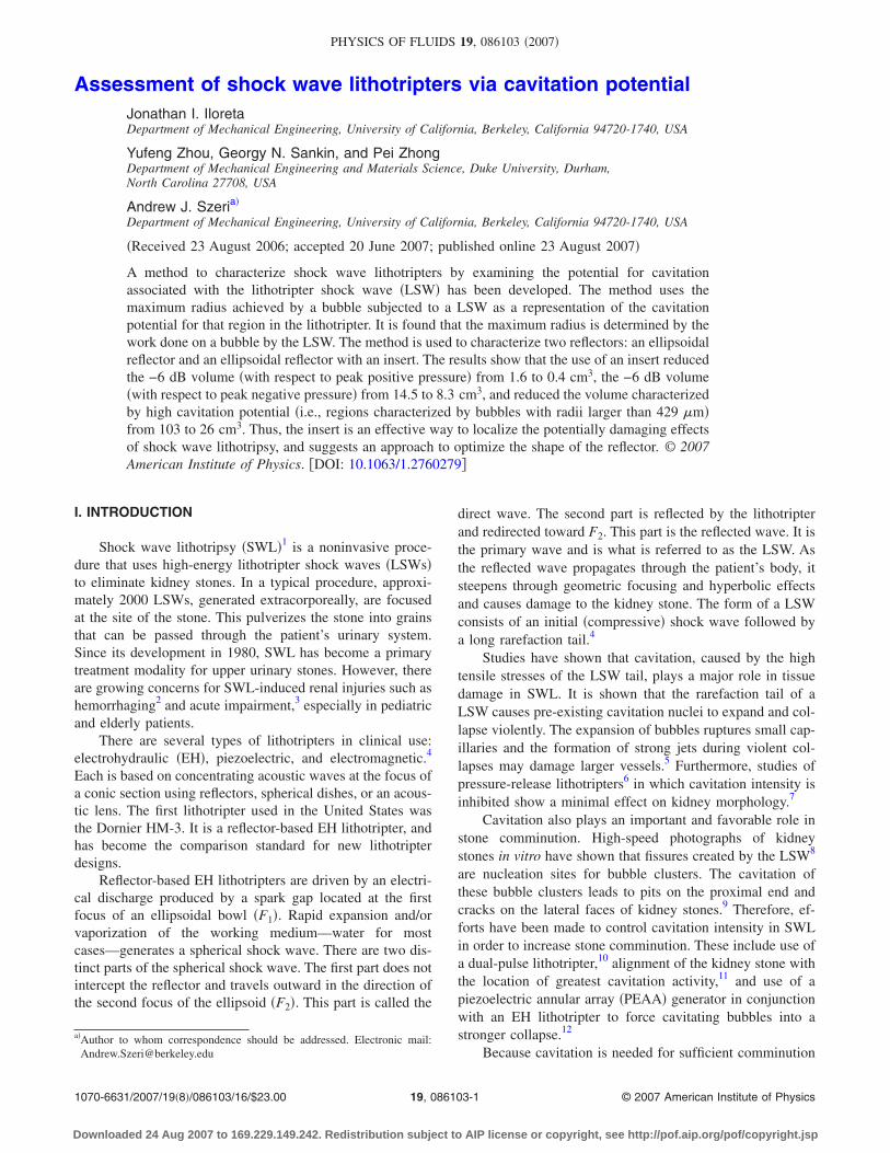
We motivate this by looking at a single spherical bubblethat is forced with the rarefaction tail of a LSW �see Fig. 1�.We only consider the rarefaction tail of the LSW here �andthroughout the rest of the paper� because our tests showedthat the short compressive part of the LSW does not affectbubble dynamics appreciably. In these tests, it was found thatincreasing the amplitude of the leading shock produced neg-ligible changes in cavitation-related parameters such as themaximum radius and peak collapse temperature. The bubbledynamics were, however, strongly dependent on the natureof the rarefaction tail of the LSW. Similar results were notedby Church.20 The tests were performed using a Rayleigh-Plesset �RP� solver that incorporated gas diffusion, heattransfer, chemical reactions, surface tension, and viscous ef-fects. The code21 was developed by Storey, and the detailscan be found in the corresponding reference. Hereinafter, thecode will be referred to as BUBBLE.

Initially the bubble is regarded as having zero energy,i.e., KE+PE=0. The kinetic energy �KE� is zero because thebubble is still and we set the potential energy �PE� to zero forreference. After the LSW does work on the bubble, thebubble gains kinetic and potential energy, the sum of whichequals the work done: W=KE+PE. The bubble then growsinertially without input from the LSW. At maximum volume,the bubble converts all of its kinetic energy into potentialenergy. Thus, the work done on the bubble is equal to thepotential energy22 of the bubble at maximum radius:

W = PE = �V0

Vmax

�p� − pb�dV . �2�

Here the bubble pressure is the sum of the vapor and gaspressures within the bubble �pb= pv+ pg� and the integral istaken along the path connecting the initial and maximumvolumes: V0 and Vmax, respectively. Because �2� requires

FIG. 1. The radial dynamics of a bubble �dashed� subjected to a typicalLSW �solid� is shown.

086103-2 Iloreta et al. Phys. Fluids 19, 086103 �2007�


knowledge of the exact volume dynamics of the bubble, itcannot be integrated to give a general equation. However, wecan learn something about the system by making a few ap-proximations. First, for bubbles subjected to LSWs, pv�pg,so pb can be replaced by pv in �2�.21 Second, Vmax�V0, soV0 can be replaced by 0. Finally, the vapor pressure is almostconstant during the expansion phase of the bubble. Thus, �2�can be approximated by

W � �0

Vmax

�p� − pv�dV = �p� − pv�4

3�rmax

3 ,

where pv is some suitable mean value of the vapor pressure.Thus, we have motivated the notion that the work done on abubble is closely related to the maximum radius the bubbleachieves.

We now turn our attention to determining a more exactrelationship between rmax and W. For this, we use BUBBLE todetermine the dynamics of bubbles subjected to LSW pulsesof the form

Pa�t� = 2Pamp cos�2f�t +�

2�exp− �� 1

12f+ t� , �3�

where Pamp, �, and f are parameters of the LSW. As definedabove, the LSW starts at the rarefaction and does not includethe leading shock wave. To add the leading shock wave to�3�, one only needs to change the phase shift of the cosineterm from � /2 to � /3. The work done on the bubble inchanging its radius from r1 to r2 �from time t1 to t2� is cal-culated using

W = �r1

r2

Fdr = �t1

t2

�P � A�rdt = 4��t1

t2

Pr2rdt , �4�

where F is the force applied on the bubble surface, A is thearea of the bubble surface, r�t� is the bubble radius, and a dotrepresents a time derivative so r�t� is the bubble wall veloc-ity. Note that the external pressure, P�t�, in �4� is given by�3� in the foregoing test. However, �4� is a general equationand is valid for any P�t�.

The test simulated argon bubbles in water using the fol-lowing properties: initial ambient pressure p0=1.01�105 Pa, initial gas pressure pg0= p0, water density �l

=996.6 kg/m3, argon molecular weight M =39.95 g/mol,water sound speed cl=1481 m/s, water surface tension �l

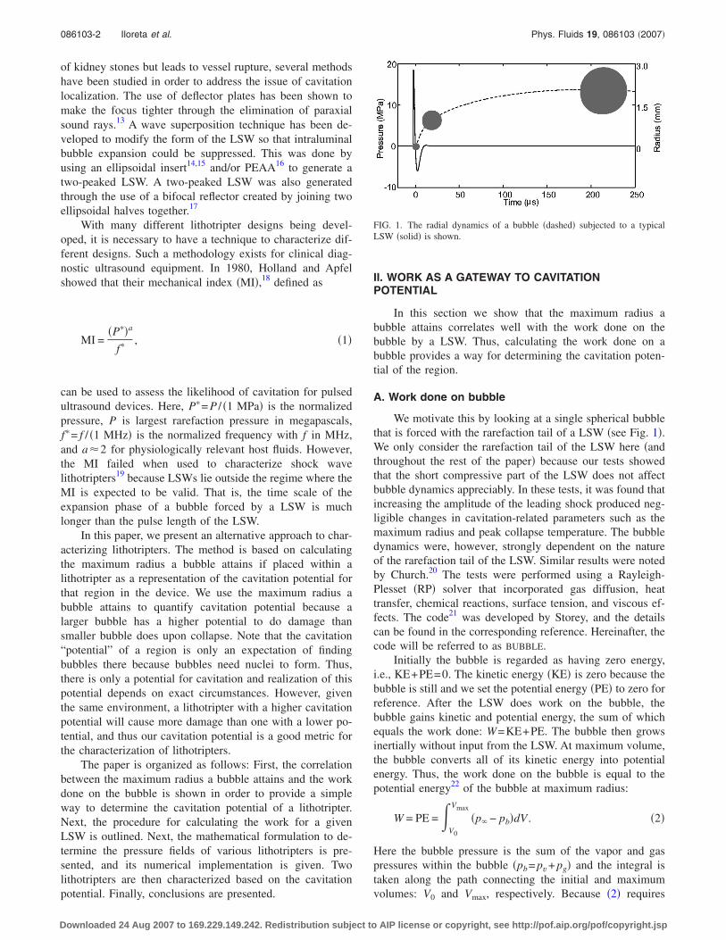
=72.8 dyn/cm, argon surface tension �g=3.418 dyn/cm, ar-gon polytropic index �=1.4, and water dynamic viscosity�l=1.00 cP. Note that argon bubbles were used for simplic-ity because the maximum radius a bubble attains when sub-jected to a LSW does not depend on the gas inside; watervapor dominates the interior contents so diffusion and com-pressible effects of the gas in the interior is of no conse-quence. The test scanned a range of the parameter space�Pamp, f ,�� that covered realistic pressure traces for typicallithotripters. In all the tests, the initial radius r0=4.5 �m wasused because rmax does not depend on r0 for the parameterstested.20 Figure 2 shows the results of the test. A fit was doneand the following relationship was found:

rmax = 1.347W0.337, �5�

where W is in millijoules and rmax is in millimeters.Before we move on, we show that the same work versus

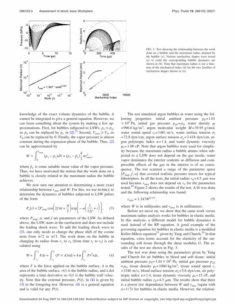
maximum radius analysis works for bubbles in elastic media.In this analysis, a different model for bubble dynamics isused instead of the RP equation. A good example of thegoverning equation for bubbles in elastic media is a modifiedKeller-Miksis equation23 given by Yang and Church.24 In thatequation, extra terms account for the elasticity of the sur-rounding soft tissue through the shear modulus G. The re-sults of the test are shown in Fig. 3.

The test was done using the parameters given by Yangand Church for air bubbles in blood and soft tissue: initialambient pressure p0=1.01�105 Pa, initial gas pressure pg0

= p0, tissue density �t=1060 kg/m3, tissue sound speed ct

=1540 m/s, blood surface tension �b=5.6 dyn/cm, air poly-tropic index �=1.4, tissue dynamic viscosity �t=15 cP, andinitial bubble radius r0=4.5 �m. The results show that thereis a power law dependence between W and rmax �again withn=1/3� for bubbles in elastic media. However, the relation-

FIG. 2. Test showing the relationship between the workdone on a bubble and the maximum radius attained bythe bubble �c�. Various rarefaction shapes were tested�a� to yield the corresponding bubble dynamics areshown in �b�. Note that maximum radius is not a func-tion of the mechanical index �d� for the two families ofrarefaction shapes shown in �a�.

086103-3 Assessment of shock wave lithotripters Phys. Fluids 19, 086103 �2007�


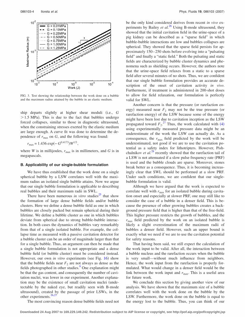
ship departs slightly at higher shear moduli �i.e., G1.5 MPa�. This is due to the fact that bubbles undergoforced collapses, similar to those in diagnostic ultrasound,when the constraining stresses exerted by the elastic mediumare large enough. A curve fit was done to determine the de-pendence of rmax on G, and the following was found:

rmax = 1.436 exp�− G0.4173�W1/3,

where W is in millijoules, rmax is in millimeters, and G is inmegapascals.

B. Applicability of our single-bubble formulation

We have thus established that the work done on a singlespherical bubble by a LSW correlates well with the maxi-mum radius an isolated single bubble attains. Now we arguethat our single bubble formulation is applicable to describingreal bubbles and their maximum radii in SWL.

There have been numerous in vitro studies25 that showthe formation of large dense bubble fields and/or bubbleclusters. Here we define a dense bubble field as one in whichbubbles are closely packed but remain spherical during theirlifetime. We define a bubble cluster as one in which bubblesdeviate from spherical due to strong bubble-bubble interac-tion. In both cases the dynamics of bubbles vary remarkablyfrom that of a single isolated bubble. For example, the col-lapse time as measured with a passive cavitation detector fora bubble cluster can be an order of magnitude larger than thatfor a single bubble. Thus, an argument can then be made thata single bubble formulation is not appropriate and a densebubble field �or bubble cluster� must be considered instead.However, our own in vitro experiments �see Fig. 16� showthat the bubble fields near F2 are not always as dense as thefields photographed in other studies.9 One explanation mightbe that the gas content, and consequently the number of cavi-tation nuclei, was lower in our experiment. Another explana-tion may be the existence of small cavitation nuclei �unde-tectable by the naked eye, but readily seen with B-modeultrasound�, created by the passage of prior LSWs, in theother experiments.26,27

The most convincing reason dense bubble fields need not

be the only kind considered derives from recent in vivo ex-periments by Bailey et al.26 Using B-mode ultrasound, theyshowed that the initial cavitation field in the urine-space of apig kidney can be described as a “sparse field” in whichbubble-bubble interactions are low and bubbles collapses arespherical. They showed that the sparse field persists for ap-proximately 150–250 shots before evolving into a “pulsatingfield” and finally a “static field.” Both the pulsating and staticfields are characterized by bubble cluster dynamics and phe-nomena such as shielding occurs. However, the authors notethat the urine-space field relaxes from a static to a sparsefield after several minutes of no shots. Thus, we are confidentthat our single bubble formulation provides an accurate de-scription of the onset of cavitation activity in vivo.Furthermore, if treatment is administered in 200-shot dosesto allow for field relaxation, our formulation is perfectlyvalid for SWL.

Another concern is that the pressure �or rarefaction en-ergy� measured near F2 may not be the true pressure �orrarefaction energy� of the LSW because some of the energymight have been lost due to cavitation inception as the LSWpropagated toward F2.27 Thus, the work calculated with �4�using experimentally measured pressure data might be anunderestimate of the work the LSW can actually do. As aconsequence, the rmax field predicted by the work will beunderestimated, not good if we are to use the cavitation po-tential as a safety index for lithotripters. However, Pish-chalnikov et al.28 recently showed that the rarefaction tail ofa LSW is not attenuated if a slow pulse frequency rate �PRF�is used and the bubble clouds are sparse. Moreover, stonesbreak better as a consequence. Thus, it is becoming increas-ingly clear that SWL should be performed at a slow PRF.Under such conditions, we are confident that our single-bubble formulation is valid.

Although we have argued that the work is expected tocorrelate well with rmax for an isolated bubble during cavita-tion onset and especially at slower PRF, one may still like toconsider the case of a bubble in a denser field. This is be-cause the presence of other growing bubbles creates a back-ground pressure field that is higher than that of the free-field.This higher pressure restricts the growth of bubbles, and thermax field predicted by the work on an isolated bubble islikely a slight overestimation of the maximum radii ofbubbles a denser field. However, such an upper bound isexactly what we need if we are to use the cavitation potentialfor safety reasons.

That having been said, we still expect the calculation ofthe work input to be valid. After all, the interaction betweena bubble nucleus and the rarefaction occurs when the bubbleis very small—without much influence from neighbors.Hence, the work input from the rarefaction is properly for-mulated. What would change in a denser field would be thelink between the work input and rmax. This is a useful areafor future work.

We conclude this section by giving another view of ouranalysis. We have shown that the maximum size of a bubblecorrelates well with the work done on the bubble by theLSW. Furthermore, the work done on the bubble is equal tothe energy lost to the bubble. Thus, you can think of our

FIG. 3. Test showing the relationship between the work done on a bubbleand the maximum radius attained by the bubble in an elastic medium.



analysis as measuring the energy of the LSW lost to bubblegrowth, and looking at such a field provides a valid way ofestimating the potential for damage.

III. BUBBLE DYNAMICS

Now we turn our attention to the procedure for determin-ing the work done on a bubble by a LSW. From �4�, we seethat the radial dynamics of a bubble is needed to get anexpression for the work. If we assume that the bubble is in anincompressible �or only mildly compressible� fluid, we canuse the RP equation to find the bubble radius.

A. Simplified Rayleigh-Plesset equation

Hilgenfeldt et al.29 define a useful form of the RP equa-tion as

�l�rr +3

2r2� = pg�r,t� − Pf�t� − p0 +

r

cl

d

dtpg�r,t� − 4�l

r

r

−2�

r, �6�

where �l is the liquid density, pg is the internal gas pressure,Pf�t� is the acoustic forcing, p0 is the ambient pressure, cl isthe liquid sound speed, �l is the liquid viscosity, and � is thesurface tension. Equation �6� can be solved numerically forany Pf�t�.

However, we wish to find a simpler model for r�t�. Thiscan be done by following the analysis of Hilgenfeldt et al.29

In their paper, the authors defined distinct phases for the RPequation in response to a spatially homogeneous, standingwave, and derived analytic expressions for the bubble dy-namics and subsequent analytical laws for parameter depen-dencies. The phases were: Rayleigh collapse, turnaround anddelayed re-expansion, afterbounces �a parametric resonance�,and expansion. In our work we are interested in the RP ap-proximation for the bubble expansion phase.

In the expansion phase of the bubble dynamics, the dy-namical pressures pacc=�lrr and pvel= �3/2��lr

2 roughly bal-ance the external pressure P�t�= Pf�t�+ p0. Thus, we onlyneed to solve the simplified RP equation

�l�rr + 32 r2� = − Pf�t� − p0 = − P�t� �7�

to calculate the bubble dynamics during the time span of theLSW.

The validity of �7� was tested against �6� using BUBBLE.We tested five different driving pressures: three LSWs of theform given by �3� and the pressures at F2 for the original andupgraded reflectors we consider in Sec. V. The three LSWswere a theoretical shock wave as defined by Matula et al.21

�Pamp=33 MPa, �=0.35 MHz, f =50 kHz�, a strong short-lived shock wave �Pamp=80.16 MPa, �=1.6 MHz, f=200 kHz�, and a weak long-lived shock wave �Pamp

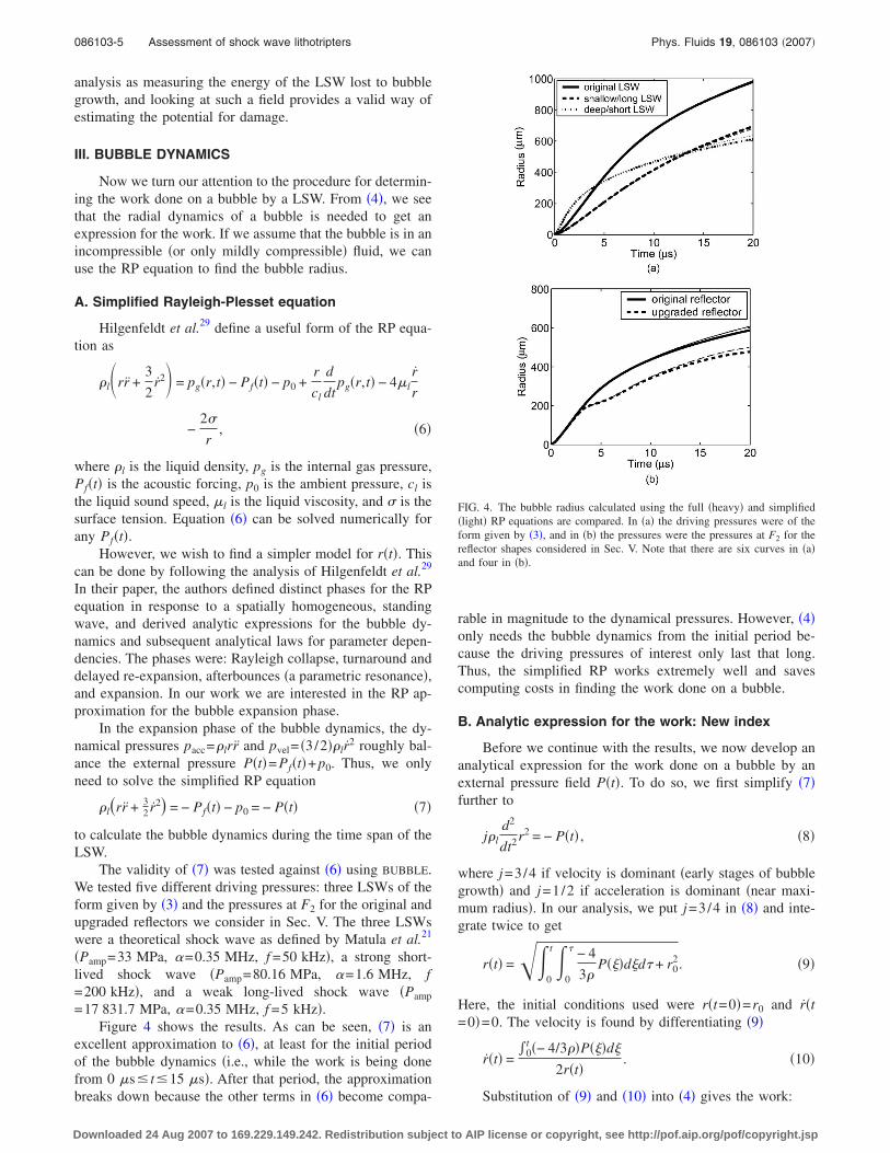
=17 831.7 MPa, �=0.35 MHz, f =5 kHz�.Figure 4 shows the results. As can be seen, �7� is an

excellent approximation to �6�, at least for the initial periodof the bubble dynamics �i.e., while the work is being donefrom 0 �s t15 �s�. After that period, the approximationbreaks down because the other terms in �6� become compa-

rable in magnitude to the dynamical pressures. However, �4�only needs the bubble dynamics from the initial period be-cause the driving pressures of interest only last that long.Thus, the simplified RP works extremely well and savescomputing costs in finding the work done on a bubble.

B. Analytic expression for the work: New index

Before we continue with the results, we now develop ananalytical expression for the work done on a bubble by anexternal pressure field P�t�. To do so, we first simplify �7�further to

j�ld2

dt2r2 = − P�t� , �8�

where j=3/4 if velocity is dominant �early stages of bubblegrowth� and j=1/2 if acceleration is dominant �near maxi-mum radius�. In our analysis, we put j=3/4 in �8� and inte-grate twice to get

r�t� = �0

t �0

� − 4

3�P��d�d� + r0

2. �9�

Here, the initial conditions used were r�t=0�=r0 and r�t=0�=0. The velocity is found by differentiating �9�

r�t� =�0

t �− 4/3��P��d�

2r�t�. �10�

Substitution of �9� and �10� into �4� gives the work:

FIG. 4. The bubble radius calculated using the full �heavy� and simplified�light� RP equations are compared. In �a� the driving pressures were of theform given by �3�, and in �b� the pressures were the pressures at F2 for thereflector shapes considered in Sec. V. Note that there are six curves in �a�and four in �b�.



W = �t1

t2 P�t�2� �0

t �0

� − 4

3�P��d�d� + r0

2

��0

t − 4

3�P��d�dt . �11�

Thus, the work can be considered a functional: W=W�P�t� ,� ,r0�. However, we can eliminate the dependenceon r0 if

r02 � �

0

t �0

� − 4

3�P��d�d� . �12�

Furthermore, if the external pressure is parametrized by onlyan amplitude Pamp and frequency f , the work scales like

W �Pamp

5/2

f3�3/2 . �13�

The constant of proportionality in �13� may bedetermined—at least approximately—for wave fields of cer-tain forms. For example, the work done on a bubble drivenby a LSW of the form of �3� for 0 t1/ �2f� and 0 for t1/ �2f� is approximated by

W �9� − 16

3�� − 2��2exp�− x0.85�

Pamp5/2

f3�3/2 ,

where x�� / f . This work index is not directly practical foruse to characterize shock wave lithotripters. Instead, it givesone an idea of how the work input varies with differentparameters.

IV. PRESSURE FIELD

To compare lithotripter designs via our cavitation poten-tial, we need a way to determine the pressure fields of thereflectors. In the past, this has been accomplished numeri-cally by several authors. Christopher30 used an acousticbeam model to determine the propagation of a LSW from aDornier HM-3 for water and tissue. However, his schemeused an arbitrary tensile strength limit to produce “reason-able looking” waveforms. Averkiou and Cleveland31 mod-eled an EH lithotripter using geometrical acoustics and theKhokhlov-Zabolotskaya-Kuznetsov �KZK� equation. Theirresults showed good comparison with experimental measure-ments, but the accuracy was limited due to the parabolicapproximation of the diffraction. Tanguay32 developed amodel of shock wave propagation in a bubbly liquid mixtureusing an ensemble-averaged, two-phase flow scheme. His re-sults also compared well with experiments, but he used awall boundary condition for the reflector. Zhou and Zhong33

developed an equivalent reflector model coupled with theKZK equation to solve for the pressure field of their originaland upgraded reflectors �see Secs. V B and V C,respectively�.

In this section, we develop a new model of SWL that canbe used to determine the pressure fields of different reflectordesigns. It is similar to the model developed by Tanguay,32

but treats the reflection problem differently. We chose to de-velop our own code for convenience and flexibility, and to

allow for comparisons of different designs using the samecode. The model described below is very simple �yet power-ful� and easily implemented by many numerical solvers toprovide qualitatively accurate pressure fields that can betested by determining the cavitation potential of the field.

A. Model formulation

In our simplified model, we consider the shock propaga-tion process to be isentropic and the flow field to be homo-geneous. The domain is taken to be axisymmetric to reducethe number of space dimensions to two. With these approxi-mations, the flow field is governed by the axisymmetric Eu-ler equations

�

�tq +

�

�rF�q� +

�

�zG�q� = S�q� , �14�

where the variables vector q, flux vectors F�q� and G�q�,and the geometric source vector S�q� are defined as

q =��

�u

�v

�e�, F�q� =�

�u

�u2 + p

�uv

��e + p�u� ,

�15�

G�q� =��v

�uv

�v2 + p

��e + p�v�, S�q� =�

−1

r�u

−1

r�u2

−1

r�uv

−1

r��e + p�u

� .

Here, ��r ,z , t� is the fluid density, u�r ,z , t� is the axial veloc-ity, v�r ,z , t� is the radial velocity, and p�r ,z , t� is thepressure.

The fourth component of �14� is the balance of mechani-cal energy per unit volume �hereinafter it will be simplyreferred to as the energy equation�. It is found by taking thescalar product between the velocity vector and the balance oflinear momentum. However, this energy balance lends nonew information �i.e., the system is still open�. It only intro-duces the total mechanical energy per unit mass �e�, definedas the sum of the kinetic energy per unit mass 1

2 �V�2= 12 �u2

+v2� and the “strain” energy per unit mass: =��p /�2�d�.The system of equations �14� is closed by specifying the

Tait equation of state �EOS�. The Tait EOS is the isentropic�p ,��-relationship for water, and if rearranged as

pTait � p + B =B + 1 atm

�0n �n, �16�



it has the same form as the equation of state for an ideal gas;i.e., p /��=const. Here, ��cp /cv is the specific heat ratio,and cp and cv are the specific heats at constant pressure andvolume, respectively. Thus, if p in �15� is replaced by pTait,our governing equations look formally like those of an idealgas, because �14� is invariant to pressure translations. Notethat although the energy equation is not invariant to pressuretranslations by itself, it is a direct consequence of the mo-mentum equation, so invariance is already assumed in itsderivation. In �16�, B and n are experimentally determinedconstants and �0 is the density at atmospheric pressure. TheTait EOS is valid for pressures up to 105 atm with B=3000 atm and n=7.34 With p= pTait, = p / ��n−1��.

It is critical to note that the isentropic assumption breaksdown when shocks are present due to irreversible processeswithin the shock. However, the normalized entropy jump fora weak shock is proportional to the cube of the normalizedpressure jump, �p� / ��c2�, where c is the sound speed. Forwater, �c2=2200 MPa and in SWL, �p��100 MPa. Thus,the isentropic assumption is a good approximation.

B. Numerical implementation

The system of equations in �14� along with �16� is solvednumerically using CLAWPACK �Conservation LAWsPACKage�.35 CLAWPACK is a collection of FORTRAN subrou-tines that solves time-dependent hyperbolic systems based onthe method of characteristics. The package is capable ofsolving nonlinear, nonconservative systems with sourceterms. The source code solves the Reimann problem betweenadjacent nodes in a finite volume mesh using a first-orderGodunov scheme with second-order corrections. This deter-mines the waves that propagate through the domain. Limiterfunctions are used to modify the second-order corrections tothese waves. The code is stable for Courant-Friedrichs-Lewynumbers CFL�max�c�t /�x��1, where c is the wavespeed, �t is the time step, �x is the grid size, and the max istaken over all coordinate directions.

In this work we use the message-passing interface �MPI�version of the two-dimensional �2D� Euler package with asource term for the cylindrical geometry. It solves the con-servation of mass, momentum, and mechanical energy for anideal gas using the MPI parallelization scheme. The sourceterms are handled with a Godunov �fractional-step� splittingtechnique in which the homogeneous problem is solved firstand the inhomogeneous next. A “monotonized centered” lim-iter is used to resolve the shock waves. This scheme has beenshown to be able to resolve the interaction of four shockwaves and a shock wave hitting a bubble exceptionallywell.35

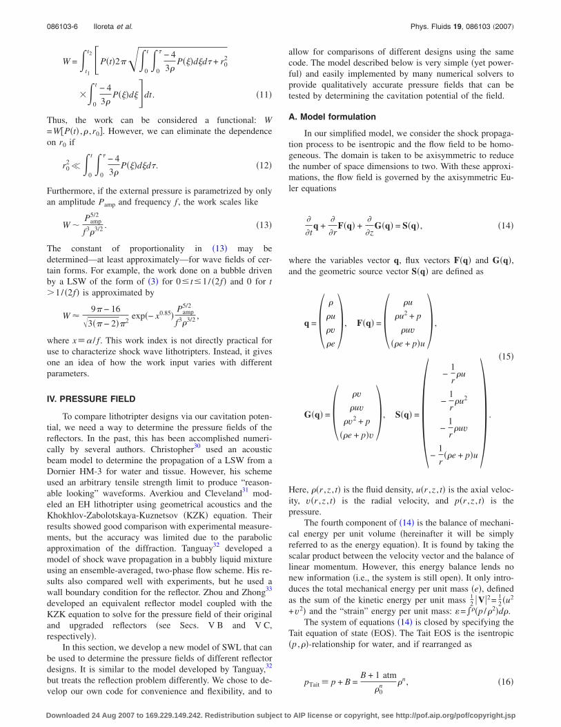
The computational domain in our work is a rectangulargrid in the axisymmetric domain; for an example, see Fig. 5.The left, top, and right boundaries are ordinary outflowboundaries, while the bottom boundary is a reflective bound-ary because it serves as the axis of symmetry for the cylin-drical domain. To ensure that the boundaries of the compu-tation domain do not affect the numerical solution, thecomputational domain is taken to be large enough such that itcontains the LSW at all times.

C. Initiation of the direct wave

The direct wave is generated by a source-like boundarycondition at F1. The source is established by specifying thetotal mechanical energy per unit volume ��e� of a ball of gridpoints surrounding F1. The idea arose by recognizing thatour mechanical energy equation is equivalent to a thermody-namic energy equation for an ideal gas. To see this we definethe total thermodynamic energy per unit mass �eth� as thesum of the internal energy per unit mass �eint� and kineticenergy per unit mass. For an isentropic process, eint is gov-erned by deint=−p dv, and for an ideal gas this yields eint

= p / ��n−1��. Therefore, eth is equivalent to e, and specify-ing the mechanical energy is equivalent to specifying thethermodynamic energy. Thus, our source creates the directwave by introducing the heat energy produced by the sparkdischarge at F1.

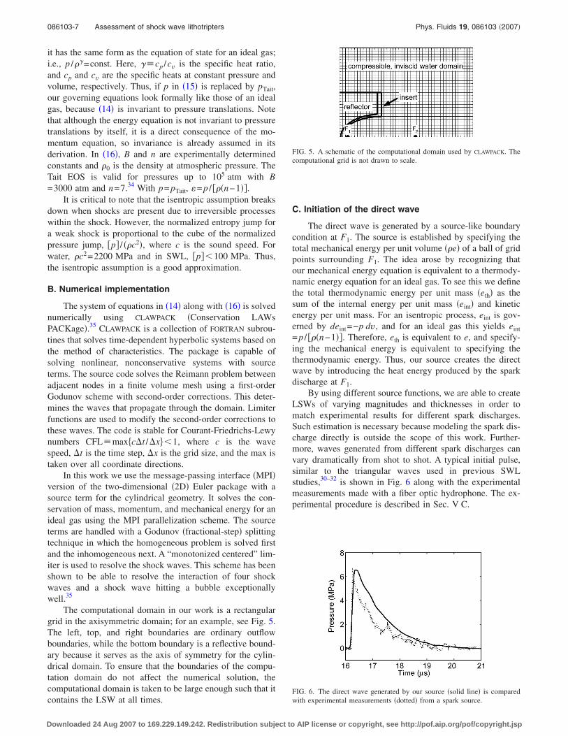
By using different source functions, we are able to createLSWs of varying magnitudes and thicknesses in order tomatch experimental results for different spark discharges.Such estimation is necessary because modeling the spark dis-charge directly is outside the scope of this work. Further-more, waves generated from different spark discharges canvary dramatically from shot to shot. A typical initial pulse,similar to the triangular waves used in previous SWLstudies,30–32 is shown in Fig. 6 along with the experimentalmeasurements made with a fiber optic hydrophone. The ex-perimental procedure is described in Sec. V C.

FIG. 5. A schematic of the computational domain used by CLAWPACK. Thecomputational grid is not drawn to scale.

FIG. 6. The direct wave generated by our source �solid line� is comparedwith experimental measurements �dotted� from a spark source.



D. Reflector

Unlike other SWL simulations32 in which a reflector ismodeled as a rigid boundary aligned with a computationalgrid, in this work the reflector and any “insert” is approxi-mated as an interface between two different regions withinthe computational domain �see Fig. 5�. The interface is de-fined by a surface such that grid cells lying within the surfaceare in the reflector domain while cells outside are in the fluiddomain. Grid cells cut by the surface are given properties ofboth domains, weighted by the volume of each domain con-tained by the grid cell. We note that a quadrilateral grid canbe used instead of a rectangular mesh to place the reflectoralong a grid line. However, this approach is not taken be-cause a rectangular mesh is accurate enough to show how thecavitation potential can be used to characterize lithotripters.

To simplify the problem, we model the solid reflectordomain as a liquid with the same EOS �but different proper-ties� as the fluid domain �see Fig. 7�. By doing so, the entirecomputational domain is governed by the same set of equa-tions and eliminates the need of coupling regions togetherwhere different equations �e.g., the Euler equations coupledwith the nonlinear elastodynamics equations� are solved. Thereflection problem is then treated by setting the properties ofthe reflector domain such that the reflection coefficient be-tween the liquid-liquid computational interface matches ana-lytical results for the reflection coefficient of an actual reflec-tor �liquid-solid interface�.

We argue that it is not necessary to solve physically ac-curate equations of motion within the reflector because onlythe reflected wave is of interest; the waves in the reflector donot directly affect the solution in the liquid. Of course, if thewaves in the reflector are subsequently re-reflected from aback side and retransmitted into the liquid domain, there isan effect on the solution. However, this is accompanied by atime delay of sufficient length so as to render the alterationof the pressure field unimportant for the present purposes.

In the analysis that follows, we first consider the liquid-solid reflection problem to determine the reflection coeffi-

cient of the lithotripter reflector, on the liquid side. We thenconsider the liquid-liquid reflection within the computationaldomain to determine the properties of the reflector domain toachieve this same reflection coefficient. In both sections,only the main results are shown; interested readers shouldconsult Refs. 37 and 38 for details.

The reflection coefficient for a plane wave incident froma liquid hitting a liquid-solid interface is given in Chap. 1.4of Brekhovskikh37 and is outlined here for convenience. Ingeneral, the velocity at any point in a solid can be expressedthrough a scalar and a vector potential. In planar problems,this is reduced to two scalar potentials, � and �, for thelongitudinal and transverse waves, respectively. These poten-tials satisfy separate wave equations with different wavespeeds given in terms of the density of the material and theLamé constants � and �. For liquids, we take � and � to bezero because liquids can only support longitudinal waves.The interface conditions are that the normal stress and dis-placement must be continuous and the tangential stress mustvanish because liquids cannot support shear. To solve thesystem of equations, harmonic wave solutions are assumedfor the potentials, and the amplitudes and wave numbers aredetermined.

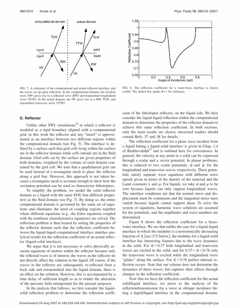
Figure 8 shows the reflection coefficient for a brass-water interface. We see that unlike the case for a liquid-liquidinterface in which the modulus is a monotonically decreasingfunction of �i �see �17� below�, the modulus for a liquid-solidinterface has interesting features due to the wave dynamicsin the solid. For �i�0.37 both longitudinal and transversewaves are excited in the solid, and for 0.37��i�0.78 onlythe transverse wave is excited while the longitudinal wave“glides” along the surface. For �i0.78 perfect internal re-flection occurs. Note that our scheme does not determine thedynamics of these waves, but captures their effects throughchanges in the reflection coefficient.

Now that we have the reflection coefficient for the actualsolid/liquid interface, we move to the analysis of thereflection/transmission for a wave at oblique incidence hit-ting a liquid/liquid interface in the computational domain.

FIG. 7. A schematic of the computational and actual reflector interface, andthe waves set up upon reflection. In the computational domain, the incidentwave �IW� gives rise to a reflected wave �RW� and transmitted longitudinalwave �TLW�. In the actual domain, the IW gives rise to a RW, TLW, andtransmitted transverse wave �TTW�.

FIG. 8. The reflection coefficient for a water-brass interface is shown�solid�. The dotted line marks R=1 for reference.



This is given in Chap. 5.B.1 of Blackstock,38 so we just citethe result. The reflection coefficient �Eq. B–9a ofBlackstock38� is given by

R �p−

p+ =Z2 cos �i − Z1 cos �t

Z2 cos �i + Z1 cos �t

=

p2

p1

�2

�1cos �i − 1 −

p2

p1sin2�i

�2

�1

p2

p1

�2

�1cos �i + 1 −

p2

p1sin2�i

�2

�1

, �17�

where p− and p+ are the strengths of the incident and re-flected waves, respectively, Zj =� jcj is the impedance of thejth medium, �i is the angle of incidence, and �t is the angleof transmission. The sound speed cj = npj /� j, and the anglesof incidence and transmission are related by Snell’s law�c1 sin �t=c2 sin �i�. Here, and throughout the rest of the pa-per, “1” refers to the working medium and “2” to thereflector.

From �17� we see that the reflection coefficient is only afunction of the pressure ratio p2 / p1, the density ratio �2 /�1,and the angle of incidence �i. Thus, we are free to vary anyor all of these parameters to change the reflection coefficientin our computational domain. In our scheme, we choose tovary only the density ratio because a pressure jump inducesmotion and the angle of incidence is fixed by the geometry ofthe lithotripter. Thus, the reflector is simply modeled as adensity jump across a prescribed boundary. The density ratio�2 /�1 is calculated using �17� for a given interface and ge-ometry. We note that this scheme is similar to the impedancemismatch method36 developed to study acoustic scattering.

The initial density of the reflector is set as follows: Thereflection coefficient for the materials of interest is calculatedas in Fig. 8. The density ratio in �17� that gives the samereflection coefficient pointwise is assigned to the interface�reflector�. The interior grid points are given the same den-sity ratio as the grid point along the surface with the sameaxial position. If the density ratio is almost infinite �i.e., R�1�, a cutoff reflection coefficient is applied such that thecode is stable with regard to the density ratio changing as afunction of time due to numerical dissipation.

Note that we only set the initial density of the reflectorand allow it to evolve according to the equations of motion.Thus, the density jump, and consequently the reflection co-efficient, of the reflector changes with time. However, wenow show that the change is negligible. From Fig. 6, theLSW has a peak pressure of about 7 MPa at 1 cm away fromF1. Therefore, the peak pressure of the LSW at the reflectoris at most 7 MPa. This is a change of 0.2% in the pressure.By �16�, the density changes 0.029%. We now determinehow these changes affect the accuracy of our reflection co-efficient. This is done by defining a modified reflection co-

efficient R and comparing it to the original reflection coeffi-

cient. To maximize the error, we define R, by setting p1

=0.998p1, p2=1.002p2, �1=0.999 71�1, and �2=1.000 29�2

in �17�. Comparing the reflection coefficients, we find that

�R−R� /R0.08% for the range of reflection coefficients inFig. 8.

V. PRESSURE FIELD RESULTS

In this section, we show the results of the pressure fieldscalculated with our model. We first present tests to validateour reflector-density scheme. We then compare the pressurefields obtained with our model with previous numerical andexperimental results for two lithotripter designs to validateour model. The designs we consider are an ellipsoidal reflec-tor and ellipsoidal reflector with an insert.

A. Code validation

The principal validation for the numerical scheme is thefollowing. Beginning with a numerical waveform thatclosely approximates experimental measurements near F1,the scheme is able to propagate forward the solution to yielda numerical waveform that closely approximates experimen-tal measurements near F2. However, we first examine thereflection technique in some detail.

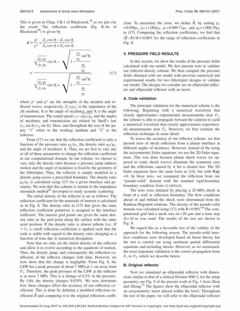
To assess the accuracy of our reflector scheme, we firstpresent tests of shock reflection from a planar interface atdifferent angles of incidence. However, instead of the usingthe axisymmetric Euler equations, we use the 2D Euler equa-tions. This was done because planar shock waves �as op-posed to conic shock waves� eliminate the symmetry axisand the reflections caused by it for a cleaner test. The 2DEuler equations have the same form as �14�, but with S�q�=0. In these tests, we compared the reflection from our“pseudo-solid” domain with the standard rigid-boundaryboundary condition from CLAWPACK.

The tests were initiated by placing a 20 MPa shock infront of a wall or reflection boundary. The flow conditionsahead of and behind the shock were determined from theRankine-Hugoniot relations. The density of the pseudo-soliddomain was calculated using �17� with R=0.993.40 The com-putational grid had a mesh size dx=20 �m and a time stepdt=10 ns was used. The results of the test are shown inFig. 9.

We regard this as a favorable test of the validity of theapproach for the following reason. The pseudo-solid inter-face conditions were developed based on linear theory, butthe test is carried out using nonlinear partial differentialequations and including shocks. However, as we mentioned,the most important validation is the correct propagation fromF1 to F2, which we describe below.

B. Original reflector

Next we simulated an ellipsoidal reflector with dimen-sions similar to that of a clinical Dornier HM-3; for the setupgeometry, see Fig. 5 of the present work or Fig. 1 from Zhouand Zhong.15 The figures show the ellipsoidal reflector withan axisymmetric insert placed within the bowl. Throughoutthe rest of the paper, we will refer to the ellipsoidal reflector



without an insert as the “original reflector” and the reflectorwith an insert as the “upgraded reflector.” In this subsectionwe consider the original reflector. In addition, the nomencla-ture for reflector parameters will follow the nomenclatureused by Zhou and Zhong.15

The original reflector we simulated had a semimajor axisa=13.8 cm, semiminor axis b=7.75 cm, and exit plane dis-tance d=12.4 cm. Here, the exit plane distance is defined asthe distance �along the semimajor axis� from the bottom ofthe reflector to the point where the reflector is truncated �theellipse is not a complete hemi-ellipsoid�. The working fluid�here and in all the other tests� was water and had an initialdensity of �1=1000 kg/m3. The brass reflector had an initialdensity calculated from the reflection coefficient given inFig. 8. The analysis used the following parameters: densityof brass �2=8600 kg/m3, longitudinal wave speed in brassc2=4073 m/s, transverse wave speed in brass b2

=2114 m/s, and sound speed in water c1=1482 m/s. As inSec. V A, R0.993 was used for stability. The source func-tion that produced the direct wave in Fig. 6 was used toinitiate the simulation.

The computational grid had a mesh size dx=39 �m andtime step dt=10 ns was used. This corresponded to a maxi-mum Courant number CFLmax=0.4066 at t=196 �s. Thesimulation, as well as the one for the upgraded reflector,were run on DataStar, the largest IBM terascale machine atthe San Diego Supercomputer Center �SDSC�.41

To show that our scheme captures the correct propaga-tion, we now turn to the pressure field of the original reflec-tor and compare it with numerical and experimental mea-surements. We first start with a comparison with numericalresults. In Fig. 10 we compare the pressure at various pointsalong the symmetry axis as calculated with the present model

FIG. 9. A comparison of the reflection of a shock using a rigid-boundaryboundary condition and our pseudo-solid is shown for two angles of inci-dence: �a� 0° and �b� 30°. The shock was initially 10 and 8.8 mm in front ofthe wall for cases �a� and �b�, respectively, and the pressures were taken2 mm in front of the wall.

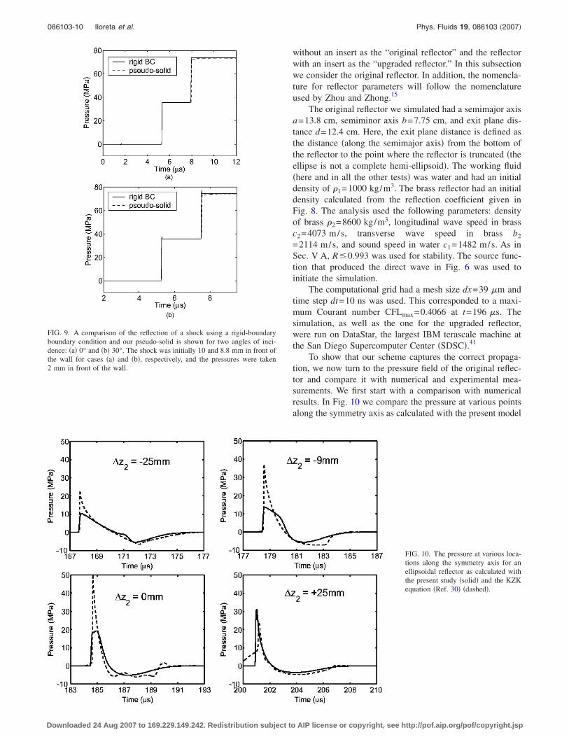
FIG. 10. The pressure at various loca-tions along the symmetry axis for anellipsoidal reflector as calculated withthe present study �solid� and the KZKequation �Ref. 30� �dashed�.



and the KZK equation.31 As readily seen, the rarefaction tailcalculated by our model and that calculated by the KZKequation have approximately the same duration and peakpressure. This agreement is exactly what we need in order tomake objective conclusions based on the results of the cal-culated rmax fields. However, the compression wave does notfocus as sharply as when modeled with the KZK equation.This can be attributed to the coarseness of the computationaldomain. In order to resolve such fine structures, the gridwould have had to be made finer. However, that would haveincreased the computational time by a factor of 3, an increasenot warranted by our goals.

We note that perfect geometric focusing is not realizeddue to nonlinear wave interactions and edge wave effects.The edge wave is a diffraction wave that emanates from theedge of the lithotripter aperture. As time �or �z2 in Fig. 10�increases the edge wave catches up to the LSW and affectsthe LSW through the steepening and expansion of the lead-ing shock wave and the rarefaction tail, respectively.

We now turn to a comparison with experimental dataobtained by Cleveland et al.39 We first show how well thepresent model simulates the propagation from F1 to F2 bycomparing focal waveform parameters that are commonlyused and defined in literature. For completeness, the defini-tions are outlined here: P±�peak positive/negative pressure;tr�rise time of the shock front, measured from 10% to 90%of the peak positive pressure; t±�positive/negative pulse du-ration, measured by the zero crossing duration of the firstpositive/negative cycle of the shock wave. Note that thesource wave and lithotripter geometries in Cleveland et al.39

are not known in detail. In the following comparison, typicalexperimental results �Anat-IU in Ref. 39� are listed in paren-theses. The peak pressures were P+=27.54 MPa �31.7 MPa�and P−=−7.39 MPa �−10.9 MPa�, the rise time was tr

=107 ns �22 ns�, and the pulse durations were t+=0.85 �s�0.85 �s� and t−=5.99 �s �4 �s�.

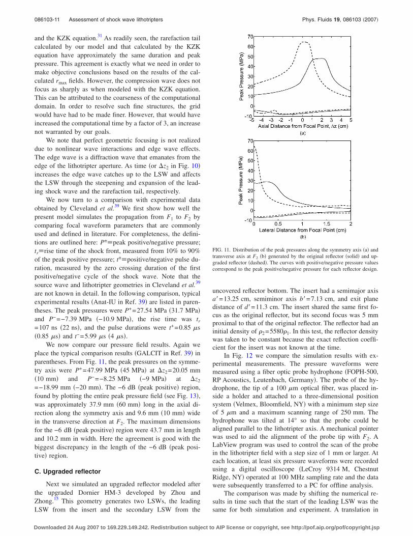
We now compare our pressure field results. Again weplace the typical comparison results �GALCIT in Ref. 39� inparentheses. From Fig. 11, the peak pressures on the symme-try axis were P+=47.99 MPa �45 MPa� at �z2=20.05 mm�10 mm� and P−=−8.25 MPa �−9 MPa� at �z2

=−18.99 mm �−20 mm�. The −6 dB �peak positive� region,found by plotting the entire peak pressure field �see Fig. 13�,was approximately 37.9 mm �60 mm� long in the axial di-rection along the symmetry axis and 9.6 mm �10 mm� widein the transverse direction at F2. The maximum dimensionsfor the −6 dB �peak positive� region were 43.7 mm in lengthand 10.2 mm in width. Here the agreement is good with thebiggest discrepancy in the length of the −6 dB �peak posi-tive� region.

C. Upgraded reflector

Next we simulated an upgraded reflector modeled afterthe upgraded Dornier HM-3 developed by Zhou andZhong.15 This geometry generates two LSWs, the leadingLSW from the insert and the secondary LSW from the

uncovered reflector bottom. The insert had a semimajor axisa�=13.25 cm, semiminor axis b�=7.13 cm, and exit planedistance of d�=11.3 cm. The insert shared the same first fo-cus as the original reflector, but its second focus was 5 mmproximal to that of the original reflector. The reflector had aninitial density of �2=5580�1. In this test, the reflector densitywas taken to be constant because the exact reflection coeffi-cient for the insert was not known at the time.

In Fig. 12 we compare the simulation results with ex-perimental measurements. The pressure waveforms weremeasured using a fiber optic probe hydrophone �FOPH-500,RP Acoustics, Leutenbach, Germany�. The probe of the hy-drophone, the tip of a 100 �m optical fiber, was placed in-side a holder and attached to a three-dimensional positionsystem �Velmex, Bloomfield, NY� with a minimum step sizeof 5 �m and a maximum scanning range of 250 mm. Thehydrophone was tilted at 14° so that the probe could bealigned parallel to the lithotripter axis. A mechanical pointerwas used to aid the alignment of the probe tip with F2. ALabView program was used to control the scan of the probein the lithotripter field with a step size of 1 mm or larger. Ateach location, at least six pressure waveforms were recordedusing a digital oscilloscope �LeCroy 9314 M, ChestnutRidge, NY� operated at 100 MHz sampling rate and the datawere subsequently transferred to a PC for offline analysis.

The comparison was made by shifting the numerical re-sults in time such that the start of the leading LSW was thesame for both simulation and experiment. A translation in

FIG. 11. Distribution of the peak pressures along the symmetry axis �a� andtransverse axis at F2 �b� generated by the original reflector �solid� and up-graded reflector �dashed�. The curves with positive/negative pressure valuescorrespond to the peak positive/negative pressure for each reflector design.



time was needed for several reasons: �1� The experimentalstart time was when the spark was ignited while the simula-tion start time was when the direct wave was already a dis-tance r0 from F1 due to the size of the source �r0 /c0

=4 mm/1459 ms−1=2.74 �s�; �2� bubbles from previousshots were not fully dissolved before the arrival of the LSWand affected the propagation of the LSW; and �3� the indi-vidual plots in Fig. 12 are for different runs and the variabil-ity of the spark discharge affected the shape of the directwave, and consequently, the waveforms near F2.

A quantitative comparison of our results with those mea-sured by Zhou and Zhong33 is made with experimental

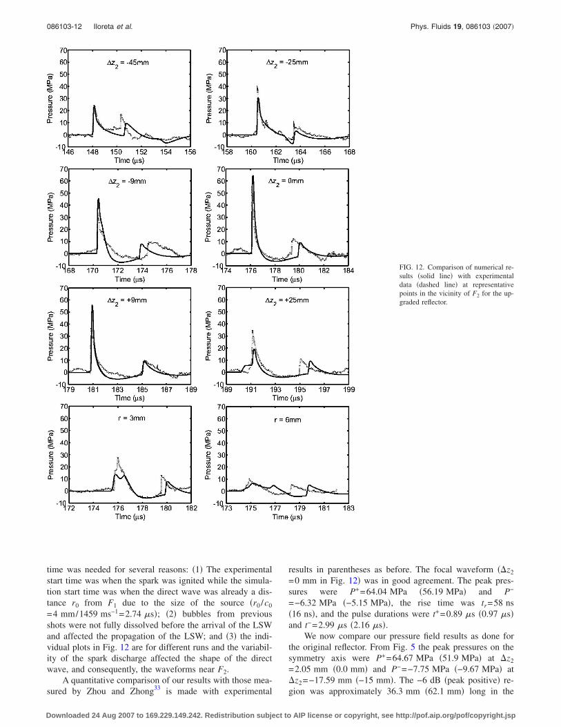
results in parentheses as before. The focal waveform ��z2

=0 mm in Fig. 12� was in good agreement. The peak pres-sures were P+=64.04 MPa �56.19 MPa� and P−

=−6.32 MPa �−5.15 MPa�, the rise time was tr=58 ns�16 ns�, and the pulse durations were t+=0.89 �s �0.97 �s�and t−=2.99 �s �2.16 �s�.

We now compare our pressure field results as done forthe original reflector. From Fig. 5 the peak pressures on thesymmetry axis were P+=64.67 MPa �51.9 MPa� at �z2

=2.05 mm �0.0 mm� and P−=−7.75 MPa �−9.67 MPa� at�z2=−17.59 mm �−15 mm�. The −6 dB �peak positive� re-gion was approximately 36.3 mm �62.1 mm� long in the

FIG. 12. Comparison of numerical re-sults �solid line� with experimentaldata �dashed line� at representativepoints in the vicinity of F2 for the up-graded reflector.



axial direction along the symmetry axis and 2.7 mm�5.9 mm� wide in the transverse direction at F2. The maxi-mum dimensions for the −6 dB �peak positive� region were36.3 mm in length and 2.9 mm in width.

VI. DISCUSSION

We now turn to the characterization of the two reflectorsin this section. We first use the peak pressure field to analyzethe flow physics. We then calculate the rmax fields using thework done on the bubbles to determine the effect reflectorgeometry has on the cavitation potential of the lithotripters.Finally, we present conclusions.

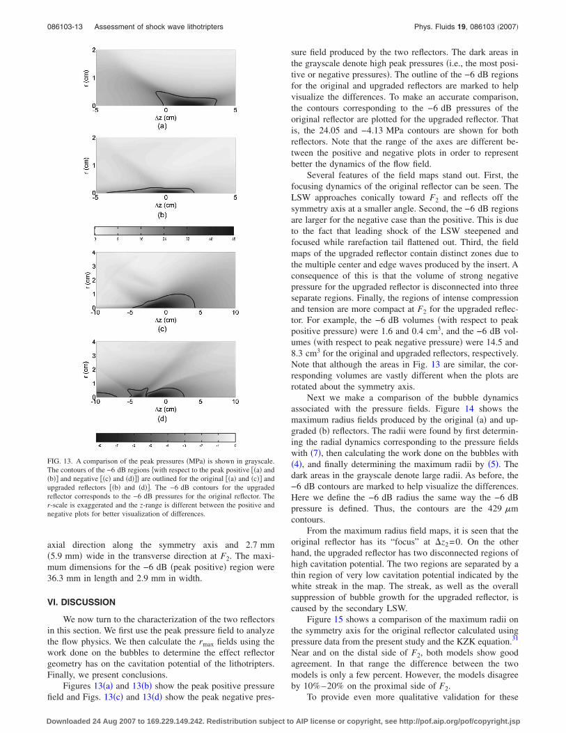
Figures 13�a� and 13�b� show the peak positive pressurefield and Figs. 13�c� and 13�d� show the peak negative pres-

sure field produced by the two reflectors. The dark areas inthe grayscale denote high peak pressures �i.e., the most posi-tive or negative pressures�. The outline of the −6 dB regionsfor the original and upgraded reflectors are marked to helpvisualize the differences. To make an accurate comparison,the contours corresponding to the −6 dB pressures of theoriginal reflector are plotted for the upgraded reflector. Thatis, the 24.05 and −4.13 MPa contours are shown for bothreflectors. Note that the range of the axes are different be-tween the positive and negative plots in order to representbetter the dynamics of the flow field.

Several features of the field maps stand out. First, thefocusing dynamics of the original reflector can be seen. TheLSW approaches conically toward F2 and reflects off thesymmetry axis at a smaller angle. Second, the −6 dB regionsare larger for the negative case than the positive. This is dueto the fact that leading shock of the LSW steepened andfocused while rarefaction tail flattened out. Third, the fieldmaps of the upgraded reflector contain distinct zones due tothe multiple center and edge waves produced by the insert. Aconsequence of this is that the volume of strong negativepressure for the upgraded reflector is disconnected into threeseparate regions. Finally, the regions of intense compressionand tension are more compact at F2 for the upgraded reflec-tor. For example, the −6 dB volumes �with respect to peakpositive pressure� were 1.6 and 0.4 cm3, and the −6 dB vol-umes �with respect to peak negative pressure� were 14.5 and8.3 cm3 for the original and upgraded reflectors, respectively.Note that although the areas in Fig. 13 are similar, the cor-responding volumes are vastly different when the plots arerotated about the symmetry axis.

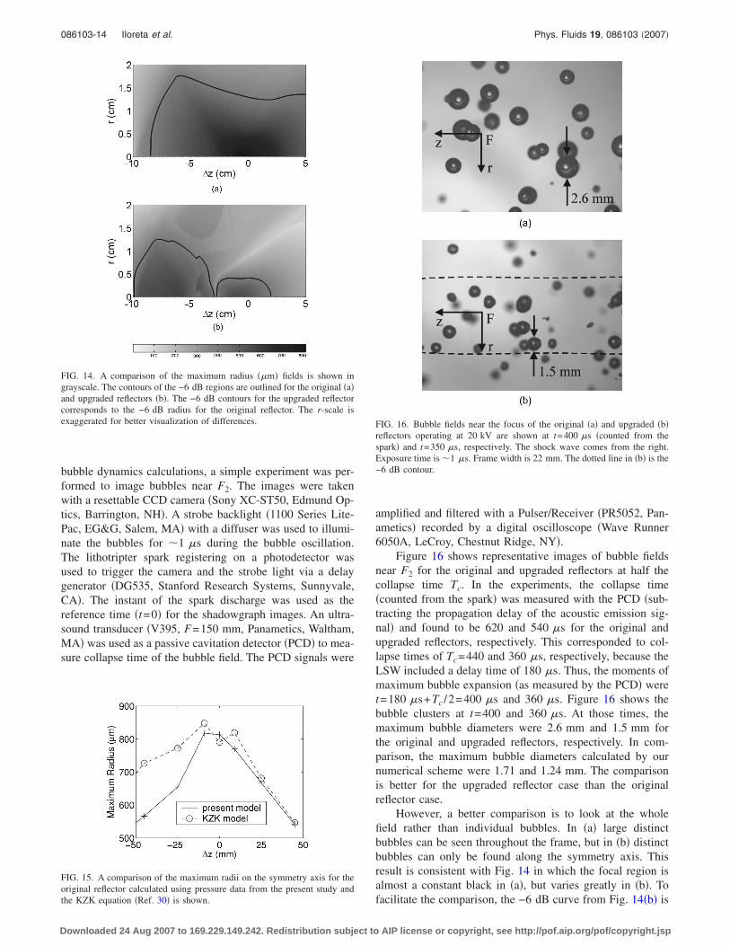
Next we make a comparison of the bubble dynamicsassociated with the pressure fields. Figure 14 shows themaximum radius fields produced by the original �a� and up-graded �b� reflectors. The radii were found by first determin-ing the radial dynamics corresponding to the pressure fieldswith �7�, then calculating the work done on the bubbles with�4�, and finally determining the maximum radii by �5�. Thedark areas in the grayscale denote large radii. As before, the−6 dB contours are marked to help visualize the differences.Here we define the −6 dB radius the same way the −6 dBpressure is defined. Thus, the contours are the 429 �mcontours.

From the maximum radius field maps, it is seen that theoriginal reflector has its “focus” at �z2=0. On the otherhand, the upgraded reflector has two disconnected regions ofhigh cavitation potential. The two regions are separated by athin region of very low cavitation potential indicated by thewhite streak in the map. The streak, as well as the overallsuppression of bubble growth for the upgraded reflector, iscaused by the secondary LSW.

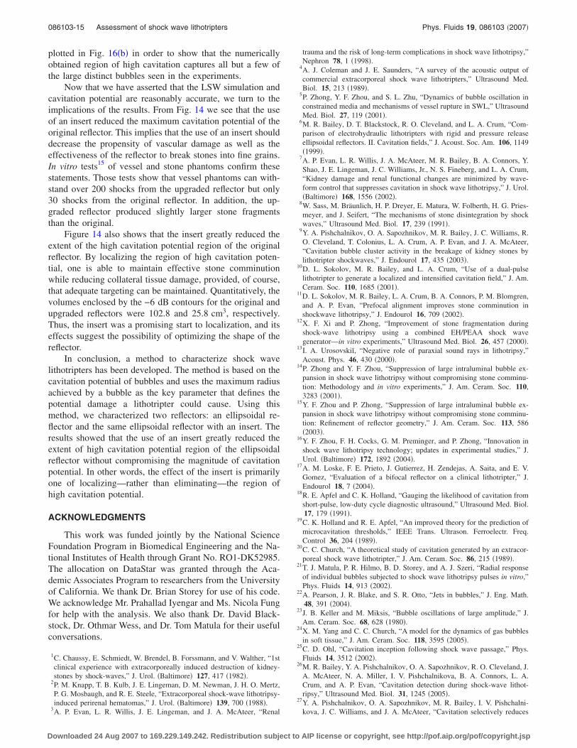
Figure 15 shows a comparison of the maximum radii onthe symmetry axis for the original reflector calculated usingpressure data from the present study and the KZK equation.31

Near and on the distal side of F2, both models show goodagreement. In that range the difference between the twomodels is only a few percent. However, the models disagreeby 10%–20% on the proximal side of F2.

To provide even more qualitative validation for these

FIG. 13. A comparison of the peak pressures �MPa� is shown in grayscale.The contours of the −6 dB regions �with respect to the peak positive ��a� and�b�� and negative ��c� and �d�� are outlined for the original ��a� and �c�� andupgraded reflectors ��b� and �d��. The −6 dB contours for the upgradedreflector corresponds to the −6 dB pressures for the original reflector. Ther-scale is exaggerated and the z-range is different between the positive andnegative plots for better visualization of differences.



bubble dynamics calculations, a simple experiment was per-formed to image bubbles near F2. The images were takenwith a resettable CCD camera �Sony XC-ST50, Edmund Op-tics, Barrington, NH�. A strobe backlight �1100 Series Lite-Pac, EG&G, Salem, MA� with a diffuser was used to illumi-nate the bubbles for �1 �s during the bubble oscillation.The lithotripter spark registering on a photodetector wasused to trigger the camera and the strobe light via a delaygenerator �DG535, Stanford Research Systems, Sunnyvale,CA�. The instant of the spark discharge was used as thereference time �t=0� for the shadowgraph images. An ultra-sound transducer �V395, F=150 mm, Panametics, Waltham,MA� was used as a passive cavitation detector �PCD� to mea-sure collapse time of the bubble field. The PCD signals were

amplified and filtered with a Pulser/Receiver �PR5052, Pan-ametics� recorded by a digital oscilloscope �Wave Runner6050A, LeCroy, Chestnut Ridge, NY�.

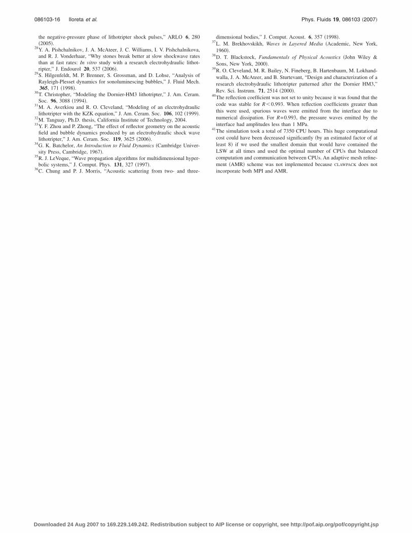
Figure 16 shows representative images of bubble fieldsnear F2 for the original and upgraded reflectors at half thecollapse time Tc. In the experiments, the collapse time�counted from the spark� was measured with the PCD �sub-tracting the propagation delay of the acoustic emission sig-nal� and found to be 620 and 540 �s for the original andupgraded reflectors, respectively. This corresponded to col-lapse times of Tc=440 and 360 �s, respectively, because theLSW included a delay time of 180 �s. Thus, the moments ofmaximum bubble expansion �as measured by the PCD� weret=180 �s+Tc /2=400 �s and 360 �s. Figure 16 shows thebubble clusters at t=400 and 360 �s. At those times, themaximum bubble diameters were 2.6 mm and 1.5 mm forthe original and upgraded reflectors, respectively. In com-parison, the maximum bubble diameters calculated by ournumerical scheme were 1.71 and 1.24 mm. The comparisonis better for the upgraded reflector case than the originalreflector case.

However, a better comparison is to look at the wholefield rather than individual bubbles. In �a� large distinctbubbles can be seen throughout the frame, but in �b� distinctbubbles can only be found along the symmetry axis. Thisresult is consistent with Fig. 14 in which the focal region isalmost a constant black in �a�, but varies greatly in �b�. Tofacilitate the comparison, the −6 dB curve from Fig. 14�b� is

FIG. 14. A comparison of the maximum radius ��m� fields is shown ingrayscale. The contours of the −6 dB regions are outlined for the original �a�and upgraded reflectors �b�. The −6 dB contours for the upgraded reflectorcorresponds to the −6 dB radius for the original reflector. The r-scale isexaggerated for better visualization of differences.

FIG. 15. A comparison of the maximum radii on the symmetry axis for theoriginal reflector calculated using pressure data from the present study andthe KZK equation �Ref. 30� is shown.

FIG. 16. Bubble fields near the focus of the original �a� and upgraded �b�reflectors operating at 20 kV are shown at t=400 �s �counted from thespark� and t=350 �s, respectively. The shock wave comes from the right.Exposure time is �1 �s. Frame width is 22 mm. The dotted line in �b� is the−6 dB contour.



plotted in Fig. 16�b� in order to show that the numericallyobtained region of high cavitation captures all but a few ofthe large distinct bubbles seen in the experiments.

Now that we have asserted that the LSW simulation andcavitation potential are reasonably accurate, we turn to theimplications of the results. From Fig. 14 we see that the useof an insert reduced the maximum cavitation potential of theoriginal reflector. This implies that the use of an insert shoulddecrease the propensity of vascular damage as well as theeffectiveness of the reflector to break stones into fine grains.In vitro tests15 of vessel and stone phantoms confirm thesestatements. Those tests show that vessel phantoms can with-stand over 200 shocks from the upgraded reflector but only30 shocks from the original reflector. In addition, the up-graded reflector produced slightly larger stone fragmentsthan the original.

Figure 14 also shows that the insert greatly reduced theextent of the high cavitation potential region of the originalreflector. By localizing the region of high cavitation poten-tial, one is able to maintain effective stone comminutionwhile reducing collateral tissue damage, provided, of course,that adequate targeting can be maintained. Quantitatively, thevolumes enclosed by the −6 dB contours for the original andupgraded reflectors were 102.8 and 25.8 cm3, respectively.Thus, the insert was a promising start to localization, and itseffects suggest the possibility of optimizing the shape of thereflector.

In conclusion, a method to characterize shock wavelithotripters has been developed. The method is based on thecavitation potential of bubbles and uses the maximum radiusachieved by a bubble as the key parameter that defines thepotential damage a lithotripter could cause. Using thismethod, we characterized two reflectors: an ellipsoidal re-flector and the same ellipsoidal reflector with an insert. Theresults showed that the use of an insert greatly reduced theextent of high cavitation potential region of the ellipsoidalreflector without compromising the magnitude of cavitationpotential. In other words, the effect of the insert is primarilyone of localizing—rather than eliminating—the region ofhigh cavitation potential.

ACKNOWLEDGMENTS

This work was funded jointly by the National ScienceFoundation Program in Biomedical Engineering and the Na-tional Institutes of Health through Grant No. RO1-DK52985.The allocation on DataStar was granted through the Aca-demic Associates Program to researchers from the Universityof California. We thank Dr. Brian Storey for use of his code.We acknowledge Mr. Prahallad Iyengar and Ms. Nicola Fungfor help with the analysis. We also thank Dr. David Black-stock, Dr. Othmar Wess, and Dr. Tom Matula for their usefulconversations.

1C. Chaussy, E. Schmiedt, W. Brendel, B. Forssmann, and V. Walther, “1stclinical experience with extracorporeally induced destruction of kidney-stones by shock-waves,” J. Urol. �Baltimore� 127, 417 �1982�.

2P. M. Knapp, T. B. Kulb, J. E. Lingeman, D. M. Newman, J. H. O. Mertz,P. G. Mosbaugh, and R. E. Steele, “Extracorporeal shock-wave lithotripsy-induced perirenal hematomas,” J. Urol. �Baltimore� 139, 700 �1988�.

3A. P. Evan, L. R. Willis, J. E. Lingeman, and J. A. McAteer, “Renal

trauma and the risk of long-term complications in shock wave lithotripsy,”Nephron 78, 1 �1998�.

4A. J. Coleman and J. E. Saunders, “A survey of the acoustic output ofcommercial extracorporeal shock wave lithotripters,” Ultrasound Med.Biol. 15, 213 �1989�.

5P. Zhong, Y. F. Zhou, and S. L. Zhu, “Dynamics of bubble oscillation inconstrained media and mechanisms of vessel rupture in SWL,” UltrasoundMed. Biol. 27, 119 �2001�.

6M. R. Bailey, D. T. Blackstock, R. O. Cleveland, and L. A. Crum, “Com-parison of electrohydraulic lithotripters with rigid and pressure releaseellipsoidal reflectors. II. Cavitation fields,” J. Acoust. Soc. Am. 106, 1149�1999�.

7A. P. Evan, L. R. Willis, J. A. McAteer, M. R. Bailey, B. A. Connors, Y.Shao, J. E. Lingeman, J. C. Williams, Jr., N. S. Fineberg, and L. A. Crum,“Kidney damage and renal functional changes are minimized by wave-form control that suppresses cavitation in shock wave lithotripsy,” J. Urol.�Baltimore� 168, 1556 �2002�.

8W. Sass, M. Bräunlich, H. P. Dreyer, E. Matura, W. Folberth, H. G. Pries-meyer, and J. Seifert, “The mechanisms of stone disintegration by shockwaves,” Ultrasound Med. Biol. 17, 239 �1991�.

9Y. A. Pishchalnikov, O. A. Sapozhnikov, M. R. Bailey, J. C. Williams, R.O. Cleveland, T. Colonius, L. A. Crum, A. P. Evan, and J. A. McAteer,“Cavitation bubble cluster activity in the breakage of kidney stones bylithotripter shockwaves,” J. Endourol 17, 435 �2003�.

10D. L. Sokolov, M. R. Bailey, and L. A. Crum, “Use of a dual-pulselithotripter to generate a localized and intensified cavitation field,” J. Am.Ceram. Soc. 110, 1685 �2001�.

11D. L. Sokolov, M. R. Bailey, L. A. Crum, B. A. Connors, P. M. Blomgren,and A. P. Evan, “Prefocal alignment improves stone comminution inshockwave lithotripsy,” J. Endourol 16, 709 �2002�.

12X. F. Xi and P. Zhong, “Improvement of stone fragmentation duringshock-wave lithotripsy using a combined EH/PEAA shock wavegenerator—in vitro experiments,” Ultrasound Med. Biol. 26, 457 �2000�.

13I. A. Urosovski�, “Negative role of paraxial sound rays in lithotripsy,”Acoust. Phys. 46, 430 �2000�.

14P. Zhong and Y. F. Zhou, “Suppression of large intraluminal bubble ex-pansion in shock wave lithotripsy without compromising stone comminu-tion: Methodology and in vitro experiments,” J. Am. Ceram. Soc. 110,3283 �2001�.

15Y. F. Zhou and P. Zhong, “Suppression of large intraluminal bubble ex-pansion in shock wave lithotripsy without compromising stone comminu-tion: Refinement of reflector geometry,” J. Am. Ceram. Soc. 113, 586�2003�.

16Y. F. Zhou, F. H. Cocks, G. M. Preminger, and P. Zhong, “Innovation inshock wave lithotripsy technology; updates in experimental studies,” J.Urol. �Baltimore� 172, 1892 �2004�.

17A. M. Loske, F. E. Prieto, J. Gutierrez, H. Zendejas, A. Saita, and E. V.Gomez, “Evaluation of a bifocal reflector on a clinical lithotripter,” J.Endourol 18, 7 �2004�.

18R. E. Apfel and C. K. Holland, “Gauging the likelihood of cavitation fromshort-pulse, low-duty cycle diagnostic ultrasound,” Ultrasound Med. Biol.17, 179 �1991�.

19C. K. Holland and R. E. Apfel, “An improved theory for the prediction ofmicrocavitation thresholds,” IEEE Trans. Ultrason. Ferroelectr. Freq.Control 36, 204 �1989�.

20C. C. Church, “A theoretical study of cavitation generated by an extracor-poreal shock wave lithotripter,” J. Am. Ceram. Soc. 86, 215 �1989�.

21T. J. Matula, P. R. Hilmo, B. D. Storey, and A. J. Szeri, “Radial responseof individual bubbles subjected to shock wave lithotripsy pulses in vitro,”Phys. Fluids 14, 913 �2002�.

22A. Pearson, J. R. Blake, and S. R. Otto, “Jets in bubbles,” J. Eng. Math.48, 391 �2004�.

23J. B. Keller and M. Miksis, “Bubble oscillations of large amplitude,” J.Am. Ceram. Soc. 68, 628 �1980�.

24X. M. Yang and C. C. Church, “A model for the dynamics of gas bubblesin soft tissue,” J. Am. Ceram. Soc. 118, 3595 �2005�.

25C. D. Ohl, “Cavitation inception following shock wave passage,” Phys.Fluids 14, 3512 �2002�.

26M. R. Bailey, Y. A. Pishchalnikov, O. A. Sapozhnikov, R. O. Cleveland, J.A. McAteer, N. A. Miller, I. V. Pishchalnikova, B. A. Connors, L. A.Crum, and A. P. Evan, “Cavitation detection during shock-wave lithot-ripsy,” Ultrasound Med. Biol. 31, 1245 �2005�.

27Y. A. Pishchalnikov, O. A. Sapozhnikov, M. R. Bailey, I. V. Pishchalni-kova, J. C. Williams, and J. A. McAteer, “Cavitation selectively reduces



the negative-pressure phase of lithotripter shock pulses,” ARLO 6, 280�2005�.

28Y. A. Pishchalnikov, J. A. McAteer, J. C. Williams, I. V. Pishchalnikova,and R. J. Vonderhaar, “Why stones break better at slow shockwave ratesthan at fast rates: In vitro study with a research electrohydraulic lithot-ripter,” J. Endourol 20, 537 �2006�.

29S. Hilgenfeldt, M. P. Brenner, S. Grossman, and D. Lohse, “Analysis ofRayleigh-Plesset dynamics for sonoluminescing bubbles,” J. Fluid Mech.365, 171 �1998�.

30T. Christopher, “Modeling the Dornier-HM3 lithotripter,” J. Am. Ceram.Soc. 96, 3088 �1994�.

31M. A. Averkiou and R. O. Cleveland, “Modeling of an electrohydrauliclithotripter with the KZK equation,” J. Am. Ceram. Soc. 106, 102 �1999�.

32M. Tanguay, Ph.D. thesis, California Institute of Technology, 2004.33Y. F. Zhou and P. Zhong, “The effect of reflector geometry on the acoustic

field and bubble dynamics produced by an electrohydraulic shock wavelithotripter,” J. Am. Ceram. Soc. 119, 3625 �2006�.

34G. K. Batchelor, An Introduction to Fluid Dynamics �Cambridge Univer-sity Press, Cambridge, 1967�.

35R. J. LeVeque, “Wave propagation algorithms for multidimensional hyper-bolic systems,” J. Comput. Phys. 131, 327 �1997�.

36C. Chung and P. J. Morris, “Acoustic scattering from two- and three-

dimensional bodies,” J. Comput. Acoust. 6, 357 �1998�.37L. M. Brekhovskikh, Waves in Layered Media �Academic, New York,

1960�.38D. T. Blackstock, Fundamentals of Physical Acoustics �John Wiley &

Sons, New York, 2000�.39R. O. Cleveland, M. R. Bailey, N. Fineberg, B. Hartenbaum, M. Lokhand-

walla, J. A. McAteer, and B. Sturtevant, “Design and characterization of aresearch electrohydraulic lithotripter patterned after the Dornier HM3,”Rev. Sci. Instrum. 71, 2514 �2000�.

40The reflection coefficient was not set to unity because it was found that thecode was stable for R�0.993. When reflection coefficients greater thanthis were used, spurious waves were emitted from the interface due tonumerical dissipation. For R=0.993, the pressure waves emitted by theinterface had amplitudes less than 1 MPa.

41The simulation took a total of 7350 CPU hours. This huge computationalcost could have been decreased significantly �by an estimated factor of atleast 8� if we used the smallest domain that would have contained theLSW at all times and used the optimal number of CPUs that balancedcomputation and communication between CPUs. An adaptive mesh refine-ment �AMR� scheme was not implemented because CLAWPACK does notincorporate both MPI and AMR.



assessment of shock wave lithotripters via cavitation ... · assessment of shock wave lithotripters...

Documents