Assessing Residual Seasonality in the U.S. National Income and Product Account Aggregates

Authors Baoline Chen, U.S. Bureau of Economic Analysis; Tucker S. McElroy and

Osbert C. Pang, U.S. Census Bureau

Date January 2021

Abstract There is an ongoing debate on whether residual seasonality is present in the

estimates of real gross domestic product (GDP) in U.S. national accounts and

whether it explains the slower quarter-one GDP growth rate in the recent

years. This paper aims to bring clarity to this topic by 1) summarizing the

techniques and methodologies used in these studies; 2) arguing for a sound

methodological framework for evaluating claims of residual seasonality; and

3) proposing three diagnostic tests for detecting residual seasonality, applying

them to different vintages and different sample spans of data on real GDP and

its major components from the U.S. national accounts and making comparisons

with results from the previous studies.

Keywords Seasonality diagnostics, residual seasonality

JEL Code C32, C51, E01

BEA Working Paper Series, WP2021-2

This paper is released to inform interested parties of research and to encourage discussion. The views expressed on the statistical issues are those of the authors and not necessarily those of the U.S. Bureau of Economic Analysis or the U.S. Census Bureau.

2

1. Introduction

There has been an ongoing debate in the public sphere as to whether residual seasonality is pres-

ent in estimates of gross domestic product (GDP) as well as its major components published by the

Bureau of Economic Analysis (BEA). This topic has stemmed from the observation that in recent

years real GDP and some of its major components from the National Income and Product Accounts

(NIPAs) have consistently grown at a lower rate in the first quarter than in the other quarters of

the year. The lower quarter-one (Q1) growth was first observed in the 1980s (Stark 2015, Lunsford

2017); it has become more persistent, and has been observed in additional GDP components in

the last two decades (Rudebusch et al. 2015, Phillips and Wang 2016, Lengerman et al. 2017, and

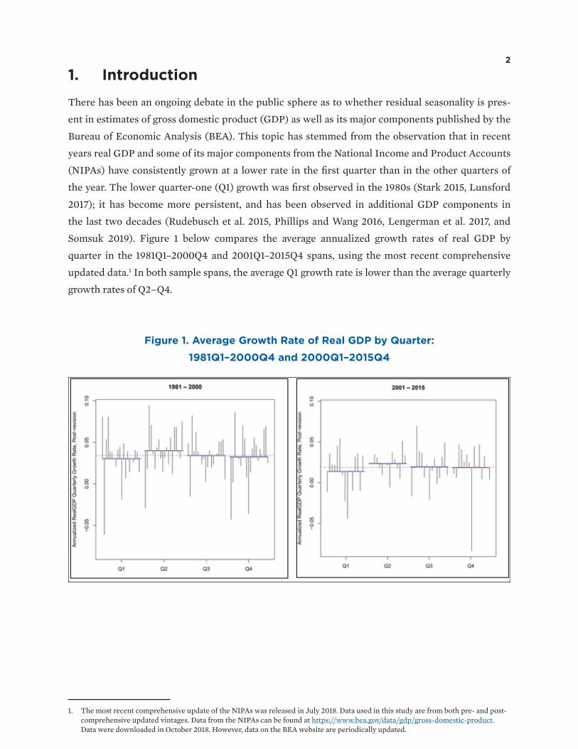
Somsuk 2019). Figure 1 below compares the average annualized growth rates of real GDP by

quarter in the 1981Q1–2000Q4 and 2001Q1–2015Q4 spans, using the most recent comprehensive

updated data.1 In both sample spans, the average Q1 growth rate is lower than the average quarterly

growth rates of Q2–Q4.

Figure 1. Average Growth Rate of Real GDP by Quarter: 1981Q1–2000Q4 and 2000Q1–2015Q4

1. The most recent comprehensive update of the NIPAs was released in July 2018. Data used in this study are from both pre- and post-comprehensive updated vintages. Data from the NIPAs can be found at https://www.bea.gov/data/gdp/gross-domestic-product. Data were downloaded in October 2018. However, data on the BEA website are periodically updated.

3

Table 1 below compares sample average growth rates of real GDP and its major components by

quarter in the 1961Q1–1980Q4 and 2001Q1–2018Q2 time spans using data after the most recent

comprehensive update of the NIPAs. In the first span, a lower Q1 growth rate is observed in only

a few components of GDP, whereas in the second span, a lower Q1 growth rate is observed in real

GDP and most of its major components.

Table 1. Average Growth Rates of Real Gross Domestic Product and Selected National Income and Product Account Aggregates, by Quarter

Variables

1961Q1–1980Q4 2001Q1–2018Q2

Q1 Q2 Q3 Q4 Q1 Q2 Q3 Q4

Real gross domestic product (GDP) 4.8 3.6 3.9 2.8 1.4 2.5 2.0 1.8

Personal consumption expenditures (PCE) 4.2 3.4 4.0 3.6 1.9 2.2 2.5 2.3

Durables 8.8 3.3 7.6 2.0 3.6 5.0 6.9 3.8

Nondurables 2.7 2.5 2.9 2.7 1.8 1.5 1.7 2.4

Services 4.0 4.0 3.9 4.7 1.6 1.9 2.1 2.0

GPDI 11.0 4.9 4.6 1.7 0.0 3.6 3.6 1.8

Structures 3.0 4.6 5.6 2.4 –3.1 5.6 0.1 –4.1

Equipment 7.4 5.3 6.9 7.9 2.2 4.4 6.3 1.9

Int. property 6.3 6.6 6.2 6.5 3.3 4.6 4.9 4.6

Residential 4.4 1.7 4.1 2.5 –0.4 1.2 –0.8 –0.1

Exports 1.9 14.7 4.2 6.2 1.7 5.1 2.5 4.8

Imports 3.8 8.4 5.7 6.7 1.7 3.3 4.1 4.2

Government 2.8 1.2 3.2 1.7 1.2 1.6 0.4 0.9

National defense 1.3 –2.0 1.4 –0.4 1.8 3.3 0.7 1.1

Nondefense 3.8 7.3 7.6 0.8 4.3 1.9 0.9 2.7

State & local government 3.8 2.6 3.3 3.9 0.3 0.9 0.1 0.4

Nominal GDP 9.4 8.2 8.6 8.4 3.2 4.6 4.1 3.6

P-Index GDP 4.7 4.7 4.8 5.3 1.8 2.1 2.0 1.8

P-Index PCE 4.7 4.7 4.9 4.8 1.8 2.1 2.0 1.3

P-Index PCE 4.2 4.6 4.7 4.6 1.8 1.8 1.6 1.7

GPDI Gross Private Domestic Investment Note: Data are from the NIPAs after the comprehensive update or benchmark revision, which was released in July 2018. The bolded entries indicate those components show lower quarter 1 growth than the other quarters.

Observations of the possible presence of residual seasonality in real GDP and its major compo-

nents were first articulated by Furman (2015), Gilbert et al. (2015), Stark (2015), Rudebusch et al.

(2015), and Groen and Russo (2015). These studies have prompted renewed interest in seasonality

diagnostics and seasonal adjustment at BEA (see the discussion in Lengerman et al. 2017). McCulla

and Smith (2015), Moulton and Cowan (2016) and Cowan et al. (2018) review some of the changes

made in response to critiques, and Phillips and Wang (2016), Lunsford (2017) and Wright (2018)

point out the continuing need for research on methodologies for detecting and removing residual

seasonality in national statistics.

4

Some of these studies report that residual seasonality has been detected in more recent years

(Furman 2015, Stark 2015, Rudebusch et al. 2015, Philips and Wang 2016, and Lunsford, 2017),

while other studies are skeptical about such a claim (Gilbert et al. 2015, Groen and Russo 2015).

Overall, the findings in each case appear to be sensitive to the methods and sample spans used.

This paper aims to bring clarity to this topic by first summarizing the techniques and methodol-

ogies used in these studies, and secondly, by arguing for sound methodological frameworks for

evaluating claims of residual seasonality. This is important, because if a statistical methodology

is applied wherein the chief axioms are violated, then any resulting claims should be treated as

dubious. We propose three diagnostic tests: 1) a model-based F (MBF) test, which tests for fixed

seasonality using seasonal dummies, but correctly accounts for time-series structure using a model

fit via generalized least squares (GLS) (Lytras et al. 2007); 2) a visual significance (VS) test, which

uses a nonparametric spectral estimator of a particular peak measure to detect peaks in the spectral

density function at seasonal frequencies corresponding to dynamic seasonality (McElroy and Roy

2021); and 3) the ROOT diagnostic test, which examines oscillatory behavior in the autocorrelation

function corresponding to the behavior of dynamic seasonality (McElroy 2021).

Our third contribution is to apply our proposed diagnostic tests to different vintages and different

sample spans of data on real GDP and its major components from the NIPAs, making comparisons

with results from the above studies. Our test results also indicate that changes made to mitigate

seasonality during the 2018 comprehensive update resulted in improvements in seasonal adjust-

ment in the U.S. national accounts. Lastly, we outline a potential solution for correcting residual

seasonality via a vast benchmarking and reconciliation system for all component series in the U.S.

national accounts.

The plan for the paper is as follows. Section 2 describes the methods used in the above- mentioned

studies and evaluates these methods according to basic criteria of diagnostics for residual season-

ality. Section 3 describes three alternative diagnostic tests proposed for detecting residual season-

ality. Section 4 reports the diagnosis of the possible presence of residual seasonality from the three

proposed diagnostic tests, using data on real GDP and its major components from the U.S. national

accounts. Section 5 reviews the findings and provides directions for future research into correcting

residual seasonality.

5

2. Methods Used for Detecting Residual Seasonality in Real GDP Estimates

Many methods are used in the above-mentioned studies: double seasonal adjustment, GLS regres-

sions, structural time-series modeling, and diagnostic tests of seasonally adjusted series. We dis-

cuss these techniques in the context of the above-cited critiques of published GDP without delving

into heavy notation; we also delineate some fallacies and limitations of these methods.

Double seasonal adjustment refers to the application of a seasonal adjustment procedure such as

X-12-ARIMA (Findley et al. 1998) to series that have already been seasonally adjusted, i.e., treat-

ing seasonally adjusted series as raw data. Rudebusch et al. (2015) apply X-12-ARIMA to identify

and estimate seasonal effects in the indirectly seasonally adjusted data from 1961Q1 to 2015Q1. The

estimated seasonal factors are shown to be nonzero, and double seasonal adjustment results in an

upward revision of Q1 growth rates as well as a downward revision of quarterly growth rates of

Q2-Q4. Gilbert et al. (2015) use the bootstrap to test the null hypothesis of zero seasonality and

applies X-12-ARIMA to identify and estimate seasonal effects in indirectly seasonally adjusted real

GDP as well as its components from 2005Q1 to 2015Q1. The bootstrap test fails to reject the null

and no residual seasonality is identified through the X-12-ARIMA procedure. Phillips and Wang

(2016) also apply X-12-ARIMA to identify and estimate seasonal effects in the indirectly season-

ally adjusted data from 1947Q1 to 2016Q1. Q1 growth rates in real GDP from 2010Q1 to 2015Q1 are

revised up via double seasonal adjustment. However, they conclude that double seasonal adjust-

ment using X-12-ARIMA may result in a poor quality adjustment in the full sample, though it can

improve the quality of seasonal adjustment if the second adjustment is only applied to the periods

where residual seasonality is significant.

Another method used in these studies is the GLS type of regression method. For example, using

seasonally adjusted data of GDP and gross domestic income (GDI) from 1959Q1 to 2014Q1, Stark

(2015) tests seasonal effects using seasonal dummies and examines the Q1 effect with signal

extraction analysis. His study finds that a low Q1 growth rate is statistically significant in the post-

1984 years, and model-based estimates using both GDP and GDI data can improve Q1 growth. In

another study, Groen and Russo (2015) test seasonal effects with seasonal dummies and lagged

GDP growth rates using data from 1975Q1 to 2015Q1. Regressions are estimated using 10-year roll-

ing windows. The results show uncorrected seasonality in the Q1s over the last 10 years of the sam-

ple, while seasonal dummies for Q2 to Q4 are never significant. To assess the impact of harsher-

than-usual winters on Q1 growth, the test is repeated by adding a new monthly weather variable

measuring monthly temperature relative to the average temperature of the current and previous

quarters. The estimates of the Q1 dummy from the second test with the weather variable included

never become significant throughout the sample.

6

Structural time series modeling is another technique employed to detect residual seasonality in

real GDP growth. Using seasonally adjusted data from 1985Q1 to 2015Q1, Lunsford (2017) decom-

poses real GDP growth into business-cycle, seasonal, and irregular components, treating the data

as seasonally unadjusted. He uses ordinary least squares (OLS) regression to estimate the cycles

(defined as fluctuations lasting 2 years and longer). He derives the seasonal component by comput-

ing the difference between GDP growth and the estimated cycles by quarter of the year, and takes

the average of the quarter-by-quarter differences between GDP growth rates and estimated cycles.

Finally, he produces confidence intervals for the quarter-by- quarter averages using low-frequency

econometrics techniques from Müller and Watson (2008, 2015) to identify regular deviations from

the business cycles that are associated with a given quarter. His analysis shows a statistically sig-

nificant average seasonal effect of –0.8 percent for the first quarter and 0.6 percent for the second

quarter during the sample span.

Another approach used in these studies is to conduct diagnostic tests on seasonally adjusted real

GDP and some major NIPA aggregates. Wright (2018) tests stable seasonality with a Wald test,2

varying seasonality with a Nyblom test (Nyblom 1989) and combined stable and moving seasonality

with a joint test. These tests are conducted on the indirectly seasonally adjusted national accounts

data using X-13ARIMA-SEATS (Census Bureau 2020) from pre- and post-comprehensive updated

vintages and on the directly seasonally adjusted data using the TRAMO-SEATS program (Gómez

and Maravall 1996). Seasonally unadjusted data were released after the 2018 comprehensive update

and date back to 2002; thus, all tests are conducted using samples from 2002Q1 to 2018Q1 so that

the results are comparable. The Wald test finds residual seasonality at the 5 percent significance

level in two components of GDP in the pre-comprehensive updated estimates (structures and fed-

eral defense), and in two components in the post-comprehensive updated estimates (structures

and equipment). The Nyblom test shows time-variation in the residual seasonality at the 5 percent

significance level in consumption, durable goods and federal defense, and at the 10 percent sig-

nificance level for the GDP price index in the pre-comprehensive updated data. In the post-com-

prehensive updated data, residual seasonality is significant at the 5 percent level only for durable

goods. With directly seasonally adjusted data, the Nyblom test finds residual seasonality significant

only for the personal consumption expenditures (PCE) price index at the 10 percent significance

level. Wright combines the Nyblom and Wald tests to test the joint null hypothesis of no fixed and

no moving residual seasonality in the NIPA estimates. The joint test is rejected at the 5 percent sig-

nificance level for structures and federal defense in the pre-comprehensive updated estimates and

for equipment in the post-comprehensive updated estimates. The joint test is not rejected in any

directly seasonally adjusted series.

2. The Wald test used in Wright (2018) is different from the F-test in X-13ARIMA-SEATS in that a lagged dependent variable is included and heteroskedasticity and autocorrelation robust standard errors are used.

7

Diagnosis of residual seasonality depends closely on the diagnostic method used. To select a proper

diagnostic for detecting the presence of residual seasonality, the first and foremost prerequisite is

to have rigorous criteria by which we judge seasonality to be present. First, a seasonality diagnostic

should distinguish between seasonal and nonseasonal processes. Second, a seasonality diagnostic

should be a statistical tool, which offers p-values or confidence intervals that can be used to quan-

tify Type I and Type II errors. Third, a seasonality diagnostic should be fully vetted against dif-

ferent types of processes and time-series data, such that the method’s performance has been thor-

oughly evaluated. Fourth, a seasonality diagnostic should treat differently seasonally adjusted (SA)

and nonseasonally adjusted (NSA), or raw, data. Seasonality in an NSA series could be deterministic

(stable), moving and stationary (dynamic), moving and nonstationary (unit-root), or a combination.

SA data has different statistical properties from NSA data: in SA data arising from a direct seasonal

adjustment, there will typically not be any deterministic or unit-root seasonality, but dynamic sea-

sonality may be present. Thus, diagnostics must take account of whether the data is NSA or SA; see

Findley et al. (2017) for additional discussion.

The choice of a seasonality diagnostic test should be determined by the type of seasonality to be

detected, and whether NSA or SA series are tested. For testing nonstationary seasonality in raw

data, commonly used tests include the HEGY diagnostic (Hylleberg et al. 1990), the Canova-

Hansen test (Canova and Hansen 1995), and the periodically integrated time-series model (Franses

1994). The advantage of the HEGY test is that it can test nonseasonal and seasonal unit roots sep-

arately. It can distinguish the presence of positive, negative, and complex unit roots in the time

series, and it determines the appropriate differencing filter for making the time series stationary.

The Canova-Hansen test is appropriate for testing the null hypothesis of deterministic seasonality

against the alternative of seasonal unit roots. The periodically integrated time-series model allows

one to test for unit roots in a framework that is more expansive than that of the HEGY test, by

allowing for seasonal heteroscedasticity.

Seasonal dummy regression models using OLS or GLS as well as the MBF test on seasonal

dummies are appropriate for testing fixed seasonality that never changes from year to year.

Additionally, the ANOVA-type (analysis of variance) methods of the Friedman (1937) and Kruskal-

Wallis (1952) tests for detecting stable seasonality are essentially seasonal-dummy regression mod-

els with the assumption of independent, identically distributed disturbances.

Spectrum diagnostics such as visual significance (VS), spectral convexity (SC) and spectral peak

(SP) are appropriate for testing fixed or dynamic periodic effects in a stationary process; see

McElroy and Roy (2021) for discussion as well as background in Priestley (1981), McElroy and

Holan (2009), and McElroy (2012). Spectrum diagnostics depict the relative contribution of dif-

ferent frequencies to the total variability in a time series. For series with prominent seasonal

8

features, the seasonal dummy estimates (calculated after appropriate temporal differencing of

the time series) correspond to local maxima at one or more seasonal frequencies in estimates of

the spectrum. The classic VS diagnostic (Soukup and Findley 1999), currently implemented in

the X-13ARIMA-SEATS program, uses an autoregressive spectrum to find “visually significant”

peaks by comparing the value of the spectrum at each seasonal frequency to its nearest neighbors,

and declaring it as a peak if the discrepancy is sufficiently large. The limitation of the original VS

approach is that it does not have any distribution theory, and hence the decision rules are ad hoc;

this weakness was corrected in McElroy and Roy (2021), where a distribution theory for a nonpara-

metric spectral estimator of peaks was derived and tested. Moreover, the X-13ARIMA-SEATS pro-

gram does not produce the spectrum for quarterly series, so VS in X-13ARIMA-SEATS is not usable

for the quarterly data in this study. In a similar spirit, the nonparametric SC diagnostic is designed

to measure and test the presence of spectral peaks by assessing their aggregate slope and convexity.

VS and SC diagnostics for detecting spectral peaks are primarily useful for detecting the presence

of residual seasonality in seasonally adjusted series.

Alternative diagnostics have been developed to detect dynamic periodic effects in a stationary pro-

cess by examining both autoregressive roots and autocorrelations at the seasonal lags. For exam-

ple, the QS diagnostic (Maravall 2012) looks for positive seasonal autocorrelation in a series, in

order to test the null hypothesis that there is no seasonality in the series. The QS diagnostic has

frequently been used for detecting residual seasonality in SA series, as it is incorporated in the pop-

ular X13ARIMA-SEATS software.

Caution must be exercised when selecting diagnostic tests for detecting residual seasonality in SA

data. NSA data may have stable and/or unit-root seasonality; therefore, unit-root tests and the MBF

test can be used. SA data will not have unit roots but might have a small degree of fixed seasonality

if the data are indirectly adjusted (that is, adjusted by aggregating SA component series), and may

exhibit dynamic seasonality. SA data may additionally also have locally nonstationary effects in the

first and last 3–5 years; this is due to edge effects occurring from the forecast extension used in the

filtering required by X-13ARIMA-SEATS program. Given these properties of SA data, we conclude

that spectral diagnostics, the MBF test, and autocorrelation diagnostics are appropriate.

OLS, as well as models of the ANOVA-type (such as the Friedman stable seasonality test and the

Kruskal-Wallis test), which assume fixed seasonality and independent and identically distributed

(i.i.d.) errors, are not proper methods for testing the presence of residual seasonality, because the

other time-series structure is ignored. The QS diagnostic only examines autocorrelation at the sea-

sonal lags, which can be high for a nonseasonal process, and thus can incorrectly declare nonsea-

sonal processes to be seasonal. Another class of diagnostics are the model-based signal diagnostics

(Blakely and McElroy 2017), which are designed for evaluating the goodness-of-fit of a model used

9

for seasonal adjustment. These are not a diagnostic for seasonality per se and cannot be applied

unless an ARIMA model has been fitted; therefore, they are excluded.

The X-11 diagnostics such as the M statistics (M7 and such) were designed by the authors of the

X-11-ARIMA program to determine whether seasonality in the raw time series can or cannot be

identified by X-11 (Lothian and Morry 1978). However, X-11 diagnostics are descriptive statistics

and do not have any known distribution theory, and therefore are not recommended for detecting

residual seasonality. Double seasonal adjustment implicitly utilizes a software program’s method-

ology for detecting seasonality; this could involve X-11 diagnostics and automatic ARIMA model-

ing, for example. When using the X-13ARIMA-SEATS program in an automatic fashion, a series is

only considered a candidate for seasonal adjustment if seasonality of the stable or unit-root types is

present; hence, SA series with residual dynamic seasonality will automatically (and fallaciously) be

regarded as nonseasonal by such a criterion.

Evaluating against the afore-described basic criteria, Rudebusch et al. (2015) and Philips and Wang

(2016) apply X-12-ARIMA to identify and estimate seasonality in the SA data, and thus, their meth-

ods inappropriately use the double SA method. The bootstrap method in Gilbert et al. (2015) utilizes

a null hypothesis of i. i. d. disturbances, which is too simplistic (being akin to the problem with using

OLS); also, the author’s use of X-12-ARIMA to identify and estimate seasonal effects suffers from the

double SA fallacy. The seasonal-dummy regression method in Stark (2015), Groen and Russo (2015)

and Lunsford (2017) fails to detect dynamic seasonality, only being suitable for stable seasonality. In

Wright (2018) the Wald test is used to test stable seasonality, and the Nyblom test, like the Canova-

Hansen test, allows for time-varying regressions to test for the presence of moving seasonality.

However, the Nyblom and Canova- Hansen tests are appropriate for testing stable versus unit-root

seasonality; they are not designed to detect dynamic seasonality, which is moving but stationary.

10

3. Alternative Diagnostics for Detecting Residual Seasonality in Real GDP Estimates

In this section we review the MBF, VS, and ROOT diagnostic tests, which are primarily treated in

Lytras et al. (2007), McElroy and Roy (2021), and McElroy (2021).

3.1 The MBF test

The framework for the MBF test assumes the data {Yt } follows a RegARIMA model (Findley et al.

1998), which is expressed as

Yt = 𝛽′xt + Zt ,

for times t = 1, … , n, where {Zt} is a seasonal ARIMA (SARIMA) model, β is the vector of regres-

sion parameters, and xt is an r-dimensional vector of regressors. If the seasonal period is s (e.g.,

s = 4 for quarterly data), then s − 1 seasonal dummies are included among the r regressors. The

SARIMA model for {Zt} accounts for stochastic dynamics such as trend, business cycle, and irreg-

ular fluctuations, but does not include seasonal differencing; this framework’s assumption is that

unit-root seasonality is not present, but instead stable (and possibly dynamic) seasonality may be

present. Such models can be fitted using maximum likelihood estimation, such as is done in the

X-13ARIMA-SEATS software. Then the Wald statistic for testing whether the regression parame-

ters are zero is

𝑊 =  ��′𝑉𝑎𝑟(𝛽)−1��.

Here, �� is the GLS estimate of 𝛽 obtained from maximum likelihood estimation, and standard for-

mulas provide the variance matrix of this estimator. Because we can always consider sub-vectors of

𝛽 in our Wald statistic, and we wish to focus upon the seasonal dummies, without loss of generality

suppose that 𝛽 in W consists only of parameters corresponding to the s − 1 = 3 seasonal dummies.

The distribution used for W relies on the fact that estimated parameters are plugged into the for-

mula for the variance of ��; denote this estimate W by W. The resulting statistic, after a rescaling, is

the MBF:

s − 1 n − dn − d − r

FM =

W

.

11

This has an F distribution on s − 1 and n − d − r degrees of freedom when 𝛽 = 0, where n is the sam-

ple size, d is the number of trend differences in the SARIMA model, r is the number of regression

parameters, and s is the seasonal period.

For testing, we take as a null hypothesis that there is no stable seasonality in the series, so that

H0: 𝛽 = 0. Note that even when H0 holds, dynamic seasonality might still be present in the SARIMA

model for {Zt }, possibly entering through a seasonal autoregressive or seasonal moving average poly-

nomial. The alternative hypothesis is that 𝛽 is nonzero, so that some degree of stable seasonality is

present. However, in neither the null nor the alternative regime can unit-root seasonality be present.

3.2 The VS test

The VS procedure of Soukup and Findley (1999) identifies dynamic seasonality when there are large

peaks in the autoregressive estimator of the spectral density at seasonal frequencies (which is just 𝜋/2

for quarterly data). The criteria used to classify a peak as large was based on ad hoc considerations

without any distribution theory to account for statistical error in estimating the spectral density.

McElroy and Roy (2021) modified the VS procedure by allowing for more flexible peak measures, by

broadening the class of spectral estimators, and by providing an asymptotic distribution theory. This

makes formal hypothesis testing of dynamic seasonality possible under the VS framework.

Suppose the time series {Yt} is stationary with no regression effects—if necessary, the SA series is

first-differenced and regression effects are subtracted. Let f be the spectral density of the station-

ary time series {Yt } (see McElroy and Politis 2020 for background), and define the left and right

peak measures at frequency θ by

log f(θ) − log f(θ − δ) log f(θ) − log f(θ + δ)

respectively, where δ > 0 parameterizes the width. The VS functional is defined as

min {log f (θ) − log f (θ − δ) , log f (θ) − log f (θ + δ)},

and is large (and positive) if and only if f(θ) greatly exceeds both its left and right neighboring values,

f(θ − 𝛿) and f(θ + 𝛿). In other words, large values of the VS function correspond to a peak at θ. The log

of the spectral density is used in order to remove the impact of scale from the asymptotic distribution.

In order to quantify the size of a peak, a fixed fraction τ of the dynamic range of the log spectrum

(that is, its maximum values minus its minimum value) is used. This is denoted τf , so that

τf = τ ∙ (max log f (λ) − min log f (λ)). λ λ

12

In Soukup and Findley (1999), the value τ = 6/52 is used, as this was found through experimenta-

tion to correspond to a fairly strong level of dynamic seasonality for a wide range of processes. The

updated VS procedure of McElroy and Roy (2021) makes use of τf to quantify peak strength, but

with τ as a tuning parameter defaulting to 0.1, and a formal hypothesis testing framework is added.

The null hypothesis is

H0: min{log f (θ) − log f (θ − δ) , log f (θ) − log f (θ + δ)} ≤ τf ,

which means that either one (or both) of the left and right peak measures are below the threshold

τf . The alternative hypothesis is

Ha: min {log f (θ) − log f (θ − δ) , log f (θ) − log f (θ + δ)} > τf ,

which indicates that a peak of magnitude τf is present at frequency θ. Note that the user chooses δ

(half of the peak’s width) and τ (the peak’s strength).

The spectral density is estimated using a nonparametric estimator, denoted by f , which is based on

tapering the sample autocovariances. An asymptotic distribution is derived that accounts for both

the taper and the bandwidth used, and 𝛼-level critical values (denoted c𝛼 ) for different tapers and

values of δ have been tabulated (using an 𝛼 of 0.05). Note that the order p = 30 autoregressive spec-

tral estimator of Soukup and Findley (1999) is not of the form of nonparametric estimators consid-

ered in McElroy and Roy (2021), and there are some other differences between the two procedures.

(The VS procedure currently in the X-13ARIMA-SEATS program also makes a comparison of the

peak functional to the median value of the spectral density estimate, and does not allow customiza-

tion of the peak width, and so forth.) In the empirical work of this paper, however, the Bartlett taper

is used (which ensures positivity of the spectral estimate, a necessity when taking logs) with band-

width ⌊n/2⌋, where n is the length of stationary time series {Yt} and ⌊∙⌋ is the integer floor function.

Substituting the nonparametric spectral estimator fˆ into the peak functional formula yields our

test statistic:

min {log f (θ) − log f (θ − δ), log f (θ) − log f (θ + δ)}.

Then H0 is rejected at level 𝛼 if the test statistic exceeds c𝛼 + τf . This criterion shows how uncer-

tainty in the spectral estimator makes it harder to reject the null hypothesis when comparing to the

case where statistical error is ignored (as in Soukup and Findley (1999)).

13

3.3 The ROOT test

The framework of the ROOT test is similar to that of VS, since we assume an invertible stationary

process {Yt} without regression effects. The AR(∞) representation of such a process is

𝜋(B)Yt = 𝜖t ,

where 𝜋(z) is a power series and {𝜖t } is white noise of variance 𝜎2. (See McElroy and Politis 2020

for background.) McElroy (2021) defines a 𝜌-persistent seasonal effect at frequency 𝜃 by the crite-

rion that 𝜋(𝜌−1𝑒𝑖𝜃) equals zero. Here 𝜌 ∈ (0,1) measures the degree of strength of seasonality, analo-

gously to 𝜏 in the VS criterion, with values closer to one indicating more persistence. Heuristically,

the persistency 𝜌 is related to the year-to-year serial correlation, but in such a way that nonseasonal

effects are accounted for.

This is a dynamic measure of seasonality, with the limiting case of 𝜌 = 1 corresponding to unit-root

seasonality. Whereas in the VS criterion peaks in the spectral density at seasonal frequencies corre-

spond to seasonality, here seasonality is assessed through oscillations in the autocovariance sequence,

and such oscillations are captured by the criterion given above. As with VS, the null hypothesis of sea-

sonality requires a choice of 𝜌, such as 𝜌 = .9 or 𝜌 = .97, and a choice of 𝜃, which is set to the same sea-

sonal frequencies used for VS. Regardless of the choice of 𝜌, the null hypothesis takes the general form

H0: 𝜋(𝜌−1𝑒𝑖𝜃) = 0.

The alternative hypothesis is simply that the criterion is some nonzero complex number, although

it is possible to get a zero value for some other choice of 𝜌. For testing, an ARMA model is identi-

fied and fitted to {Yt }, and ��(z) is computed from the maximum likelihood estimates of the param-

eters. Our own implementation fits an AR model identified by AIC, and with parameter estimates

computed via OLS. Then the test statistic of H0 is

n |��(𝜌−1ei𝜃)|2,

which under the null hypothesis has an asymptotic distribution given by a weighted sum of

squared normal random variables. Thus, large values of the test statistic indicate rejection of sea-

sonality of persistence 𝜌; we reject H0 when the test statistic exceeds the critical value (which is

obtained by Monte Carlo simulation). However, it is possible that a greater or lesser persistence of

seasonality could still be present, so we should test across many values of 𝜌. We consider testing

a null hypothesis for each 𝜌 ∈ [.98, 1), so that if all these hypotheses are rejected, we can conclude

there is no seasonality of such persistency present.

14

4. Diagnosis of Possible Presence of Residual Seasonality in Real GDP Estimates

The proposed MBF test for detecting stable seasonality as well as the VS and ROOT diagnostics for

detecting dynamic seasonality are applied to test for the possible presence of residual seasonality

in the SA estimates of real GDP and its major components in the U.S. national accounts. During the

2018 comprehensive update, some changes were made to improve the seasonal adjustment meth-

ods used in calculating real GDP. Thus, in this study, data from both pre- and post-comprehensive

update vintages are tested. Twenty series are selected, which include real GDP and its 15 major

components, nominal GDP, price index for GDP, and price indexes for PCE, and PCE excluding

food and energy. (See table 1 for the list of components included for the tests.)

Because the lower Q1 growth was first observed in the 1980s and has become more persistent in

the last two decades, our tests include quarterly data from 1980Q1 to 2015Q4, a total of 144 obser-

vations. Data from 2016 to 2018 are not included in the tests to avoid potential nonstationarity in

the series due to the edge effect occurring from forecast extension used in the filtering required by

the X-11 program. Since results from seasonality diagnostics can be sensitive to the sample size, our

tests are conducted using 20- and 15-year sample spans. Using a 4-quarter rolling window, seven-

teen 20-year sample spans (1980Q1–1999Q4, 1981Q1–2000Q4, etc.) and twenty-two 15-year sample

spans are constructed from the 144 observations. Data used in the tests are the log-transformed

original SA estimates from the U.S. national accounts.

4.1 Results from MBF Test for Detecting Stable Seasonality

Using X-13ARIMA-SEATS, a model was identified for the data over a given span using the automdl

spec, without disabling outlier detection or regression testing for other variables. The MBF test

was then performed by re-estimating the data using that model form (with some conditions men-

tioned below) with a forcibly included fixed seasonal regressor, while potentially allowing the out-

liers and other regressors to vary. The fixed seasonal regressor is then tested for significance.

There are some considerations involved, however. First, because the fixed seasonal regressor can-

not be included in a model that already contains a seasonal difference, if the model originally iden-

tified by automdl has a seasonal difference, then that seasonal difference is eliminated in the model

used for re-estimating. E.g., if automdl favors a (0 1 1)(1 1 0) form for the data, then the model used

for estimating with a fixed seasonal regressor will have a (0 1 1)(1 0 0) form.

Second, when a model has both a seasonal difference and a seasonal moving average parameter, if

the seasonal moving average parameter is close to 1, these two effectively cancel each other out.

15

Therefore, if automdl decides on a seasonal component of the form (P 1 1) and the estimated sea-

sonal moving average parameter is at least 0.98, then both the seasonal difference and the seasonal

moving average parameter will be eliminated in the model used for re-estimating, making the sea-

sonal component (P 0 0). E.g., if automdl favors a (0 1 0)(0 1 1) form for the data, but the estimated

seasonal moving average parameter is 0.999, then the model used for estimating with a fixed sea-

sonal regressor will have a (0 1 0) form.

Using the seventeen 20-year sample spans from the pre-comprehensive update estimates, the MBF

test results show the possible presence of stable seasonality at the 5 percent significance level in

6 sample spans of real GDP from 1990Q1–2014Q4; 14 sample spans of government expenditure;

16 sample spans of national defense; 7 sample spans of residential investment; 6 sample spans of

structure investment; 4 sample spans of nondurable goods, services, and exports; and 3 sample

spans of price index for GDP. Using the comprehensive updated data, the MBF test results show a

decrease in the number of spans with a possible presence of residual seasonality from 6 to 4 in real

GDP, from 14 to 2 in government expenditures, from 16 to 6 in national defense, from 3 to 1 in price

index for GDP, from 4 to 0 in exports, and from 3 to 0 in state and local government. The numbers

of sample spans that show a possible presence of stable seasonality remain unchanged for structure

investment and residential investment. However, the number of spans that show a possible pres-

ence of residual seasonality increases from 4 to 5 in nondurables, from 4 to 6 in services, and from 1

to 2 in price index for PCE.

Table 2-a below shows the p-values from the MBF test for stable seasonality in real GDP and its

major components that have shown the possible presence of residual seasonality at the 5 percent

significance level in the 20-year sample spans. For each component, p-values from the MBF test

using data before and after the comprehensive update are compared. Comparing with data before

the comprehensive update, fewer components and fewer sample spans exhibit the possible pres-

ence of stable seasonality in the estimates after the comprehensive update.

Using the 15-year sample spans in the MBF test, 15 out of the 20 series tested possible presence

of stable seasonality in some sample spans before the comprehensive update and 16 series after

the comprehensive update. Table 2-b compares the p-values from the MBF test using data before

and after the comprehensive update. MBF test results using data before the comprehensive update

show the possible presence of stable seasonality at the 5 percent significance level in 4 sam-

ple spans of real GDP; 11 sample spans of government expenditure; 20 sample spans of national

defense; 7 sample spans of residential investment; 6 sample spans of structures; and 5 sample spans

of services, exports, and state and local government. Possible presence of stable seasonality is also

identified in nondurable goods, intellectual property, imports, nominal GDP, price index for GDP,

price indexes for PCE, and core PCE in 1 to 4 sample spans.

16

Table 2-a. P-values of MBF Test for Stable Residual Seasonality in Real Gross Domestic Product and Its Major Components Using Data Before and After Comprehensive Update: 20-Year Sample Spans

Sample span

Real gross domestic product  

Nondurables Services Structures Residential Exports Federal government  

National defense

State and local

government

Personal income gross

domestic product

Personal income

personal consumption expenditures

Pre-update

Post-update

Pre-update

Post-update

Pre-update

Post-update

Pre-update

Post-update

Pre-update

Post-update

Pre-update

Post-update

Pre-update

Post-update

Pre-update

Post-update

Pre-update

Post-update

Pre-update

Post-update

Pre-update

Post-update

1980Q1–1999Q4 0.42 0.53 0.91 0.91 0.32 0.20 0.34 0.34 0.00 0.00 0.18 0.20 0.06 0.21 0.11 0.32 0.73 0.83 0.41 0.74 0.00 0.00

1981Q1–2000Q4 0.14 0.22 0.49 0.49 0.01 0.00 0.61 0.62 0.00 0.00 0.53 0.25 0.02 0.07 0.00 0.01 0.87 0.87 0.52 0.49 0.87 0.84

1982Q1–2001Q4 0.06 0.09 0.10 0.11 0.02 0.00 0.78 0.91 0.08 0.08 0.67 0.45 0.02 0.10 0.00 0.00 0.92 0.86 0.12 0.40 0.90 0.86

1983Q1–2002Q4 0.17 0.24 0.04 0.04 0.02 0.01 0.91 0.89 0.05 0.05 0.41 0.50 0.01 0.10 0.02 0.01 0.82 0.90 0.10 0.57 0.66 0.65

1984Q1–2003Q4 0.12 0.17 0.22 0.51 0.06 0.03 0.78 0.78 0.17 0.17 0.23 0.41 0.00 0.05 0.01 0.10 0.91 0.83 0.32 0.80 0.81 0.83

1985Q1–2004Q4 0.15 0.20 0.26 0.31 0.01 0.00 0.26 0.27 0.00 0.00 0.32 0.51 0.29 0.09 0.00 0.01 0.90 0.73 0.17 0.74 0.90 0.88

1986Q1–2005Q4 0.17 0.28 0.04 0.05 0.11 0.00 0.31 0.31 0.00 0.00 0.16 0.58 0.02 0.21 0.01 0.17 0.64 0.56 0.09 0.79 1.00 0.96

1987Q1–2006Q4 0.24 0.27 0.02 0.04 0.25 0.32 0.00 0.00 0.00 0.00 0.39 0.54 0.03 0.71 0.00 0.48 0.52 0.44 0.04 0.51 0.92 0.98

1988Q1–2007Q4 0.20 0.35 0.00 0.01 0.43 0.24 0.52 0.47 0.00 0.00 0.27 0.50 0.03 0.50 0.00 0.08 0.80 0.93 0.02 0.61 0.93 0.82

1989Q1–2008Q4 0.13 0.25 1.00 0.34 0.42 0.34 0.32 0.32 0.10 0.10 0.41 0.39 0.03 0.35 0.00 0.02 0.88 0.96 0.02 0.53 0.82 0.82

1990Q1–2009Q4 0.02 0.05 0.66 0.58 0.44 0.20 0.14 0.15 0.24 0.24 0.12 0.27 0.01 0.62 0.03 0.08 0.80 0.86 0.11 0.67 0.72 0.72

1991Q1–2010Q4 0.02 0.05 0.00 0.24 0.61 0.29 0.04 0.04 0.59 0.59 0.10 0.22 0.00 0.12 0.03 0.06 0.05 0.71 0.23 0.00 0.84 0.72

1992Q1–2011Q4 0.00 0.01 0.10 0.03 0.72 0.32 0.04 0.04 0.28 0.29 0.00 0.19 0.00 0.18 0.00 0.06 0.07 0.36 0.24 0.23 0.93 0.49

1993Q1–2012Q4 0.01 0.02 0.15 0.06 0.55 0.38 0.07 0.08 0.86 0.86 0.00 0.18 0.00 0.09 0.00 0.08 0.05 0.26 0.13 0.71 0.92 0.21

1994Q1–2013Q4 0.02 0.06 0.11 0.08 0.90 0.86 0.02 0.03 0.93 0.91 0.13 0.30 0.19 0.08 0.00 0.04 0.05 0.35 0.16 0.81 0.63 0.01

1995Q1–2014Q4 0.02 0.07 0.12 0.05 0.98 0.85 0.03 0.02 0.87 0.88 0.00 0.16 0.00 0.04 0.00 0.07 0.03 0.19 0.18 0.75 0.69 0.79

1996Q1–2015Q4 0.07 0.08 0.74 0.04 0.83 0.77 0.02 0.00 0.28 0.18 0.00 0.07 0.00 0.02 0.00 0.10 0.03 0.17 0.34 0.44 0.99 0.99

Note: Bolded entries show seasonality from the tests.

17

Table 2-b. P-values of MBF Test for Stable Residual Seasonality in Real GDP and Its Major Components Using Data before and after Comprehensive Update: 15-Year Sample Spans

Sample span

Real gross domestic product  

Durables Nondurables Services Gross private domestic

investment 

Structures Intellectual property

Residential Exports

Pre-update

Post-update

Pre-update

Post-update

Pre-update

Post-update

Pre-update

Post-update

Pre-update

Post-update

Pre-update

Post-update

Pre-update

Post-update

Pre-update

Post-update

Pre-update

Post-update

1980Q1–1994Q4 0.62 0.70 0.23 0.23 0.97 0.97 0.29 0.80 0.58 0.59 0.28 0.28 0.00 0.00 0.00 0.00 0.41 0.42

1981Q1–1995Q4 0.46 0.55 0.18 0.18 0.09 0.09 0.02 0.06 0.65 0.66 0.58 0.58 0.00 0.00 0.00 0.00 0.76 0.76

1982Q1–1996Q4 0.17 0.32 0.89 0.89 0.74 0.75 0.06 0.06 0.43 0.43 0.73 0.73 0.11 0.14 0.00 0.00 0.74 0.74

1983Q1–1997Q4 0.24 0.35 0.40 0.40 0.18 0.18 0.00 0.01 0.08 0.07 0.76 0.76 0.12 0.16 0.00 0.00 0.41 0.41

1984Q1–1998Q4 0.30 0.38 0.45 0.45 0.23 0.23 0.40 0.38 0.27 0.23 0.72 0.73 0.28 0.35 0.20 0.20 0.19 0.19

1985Q1–1999Q4 0.45 0.57 0.73 0.73 0.96 0.96 0.55 0.56 0.30 0.28 0.49 0.49 0.79 0.79 0.00 0.00 0.37 0.49

1986Q1–2000Q4 0.27 0.35 0.54 0.54 0.00 0.00 0.52 0.00 0.34 0.32 0.00 0.00 0.43 0.50 0.00 0.00 0.52 0.47

1987Q1–2001Q4 0.03 0.04 0.79 0.79 0.29 0.29 0.00 0.00 0.32 0.27 0.56 0.57 0.62 0.55 0.00 0.00 0.02 0.00

1988Q1–2002Q4 0.08 0.10 0.16 0.12 0.96 0.97 0.36 0.00 0.52 0.41 0.64 0.65 0.78 0.75 0.49 0.49 0.54 0.10

1989Q1–2003Q4 0.15 0.18 0.67 0.63 0.48 0.57 0.50 0.38 0.65 0.51 0.52 0.53 0.77 0.73 0.33 0.33 0.69 0.80

1990Q1–2004Q4 0.04 0.06 0.15 0.14 0.89 0.49 0.18 0.00 0.46 0.33 0.06 0.06 0.98 0.97 0.08 0.08 0.37 0.62

1991Q1–2005Q4 0.18 0.12 0.82 0.73 0.11 0.15 0.20 0.37 0.65 0.56 0.12 0.14 0.62 0.50 0.36 0.36 0.38 0.69

1992Q1-–2006Q4 0.22 0.27 0.71 0.74 0.97 0.12 0.88 0.74 0.78 0.59 0.20 0.20 0.12 0.09 0.57 0.57 0.10 0.62

1993Q1–2007Q4 0.28 0.33 0.70 0.52 0.16 0.09 0.71 0.57 0.79 0.80 0.33 0.37 0.19 0.29 0.25 0.25 0.27 0.45

1994Q1–2008Q4 0.10 0.16 0.28 0.21 0.29 0.03 0.68 0.83 0.69 0.72 0.16 0.16 0.26 0.43 0.24 0.24 0.61 0.89

1995Q1–2009Q4 0.07 0.69 0.51 0.46 0.29 0.14 0.90 0.87 0.84 0.00 0.19 0.21 0.91 0.35 0.46 0.46 0.02 0.20

1996Q1–2010Q4 0.06 0.14 0.16 0.03 0.27 0.12 0.99 0.47 0.66 0.57 0.05 0.06 0.68 0.96 0.57 0.56 0.03 0.11

1997Q1–2011Q4 0.03 0.09 0.70 0.61 0.57 0.02 0.85 0.28 0.60 0.51 0.02 0.02 0.57 0.48 0.66 0.66 0.03 0.24

1998Q1–2012Q4 0.04 0.08 0.62 0.70 0.58 0.03 0.98 0.65 0.44 0.33 0.07 0.10 0.81 0.39 0.97 1.00 0.04 0.18

1999Q1–2013Q4 0.27 0.33 0.96 0.76 0.43 0.45 0.62 0.95 0.39 0.36 0.03 0.03 0.77 0.69 0.35 0.33 0.09 0.27

2000Q1–2014Q4 0.16 0.30 0.80 0.95 0.35 0.36 0.03 0.60 0.26 0.08 0.04 0.02 0.78 0.54 0.99 0.45 0.10 0.18

2001Q1–2015Q4 0.34 0.68 0.76 0.86 0.20 0.13 0.00 0.59 0.24 0.26 0.03 0.01 0.60 0.25 0.98 0.93 0.04 0.09

Note: Bolded entries show seasonality from the tests.

18

Table 2-b. P-values of MBF Test for Stable Residual Seasonality in Real GDP and Its Major Components Using Data before and after Comprehensive Update: 15-Year Sample Spans (Cont.)

Sample span

Imports Federal government  

National defense Nondefense State & Local Nominal GDP Personal income gross domestic

product

Personal income personal

consumption expenditures

Personal income core personal consumption expenditures

Pre-update

Post-update

Pre-update

Post-update

Pre-update

Post-update

Pre-update

Post-update

Pre-update

Post-update

Pre-update

Post-update

Pre-update

Post-update

Pre-update

Post-update

Pre-update

Post-update

1980Q1–1994Q4 0.07 0.07 0.37 0.54 0.00 0.39 0.71 0.37 0.35 0.33 0.57 0.49 0.36 0.58 0.32 0.28 0.84 0.88

1981Q1–1995Q4 0.10 0.10 0.33 0.46 0.04 0.13 0.56 0.62 0.73 0.70 0.53 0.44 0.68 0.38 0.80 0.78 0.70 0.66

1982Q1–1996Q4 0.01 0.01 0.26 0.43 0.12 0.33 0.37 0.72 0.96 0.95 0.30 0.34 0.17 0.36 0.84 0.83 0.23 0.19

1983Q1–1997Q4 0.51 0.51 0.12 0.21 0.00 0.17 0.64 0.99 0.93 1.00 0.46 0.48 0.08 0.42 0.79 0.77 0.62 0.27

1984Q1–1998Q4 0.74 0.74 0.05 0.11 0.01 0.08 0.72 0.45 0.93 0.96 0.83 0.47 0.64 0.76 0.86 0.86 0.39 0.34

1985Q1–1999Q4 0.67 0.75 0.43 0.41 0.01 0.01 0.57 0.58 0.95 0.95 0.00 0.65 0.73 0.79 0.73 0.75 0.55 0.48

1986Q1–2000Q4 0.97 0.98 0.03 0.12 0.00 0.02 0.48 0.40 0.85 0.69 0.00 0.29 0.40 0.72 0.96 0.98 0.24 0.27

1987Q1–2001Q4 0.87 0.80 0.23 0.41 0.00 0.01 0.19 0.32 0.47 0.40 0.00 0.02 0.17 0.38 0.00 0.00 0.24 0.22

1988Q1–2002Q4 0.84 0.72 0.51 0.32 0.00 0.01 0.15 0.51 0.65 0.61 0.04 0.05 0.19 0.50 0.00 0.00 0.42 0.38

1989Q1–2003Q4 0.00 0.78 0.68 0.08 0.00 0.01 0.09 0.20 0.90 0.80 0.23 0.17 0.15 0.60 0.51 0.50 0.33 0.39

1990Q1–2004Q4 0.87 0.81 0.02 0.25 0.00 0.01 0.24 0.50 0.93 0.73 0.11 0.08 0.16 0.05 0.90 0.89 0.32 0.41

1991Q1–2005Q4 0.54 0.80 0.02 0.73 0.04 0.11 0.41 0.67 0.63 0.83 0.37 0.23 0.28 0.92 0.99 0.98 0.36 0.32

1992Q1–2006Q4 0.25 0.66 0.70 0.86 0.14 0.10 0.42 0.44 0.41 0.70 0.48 0.31 0.14 0.92 0.95 0.84 0.13 0.17

1993Q1–2007Q4 0.65 0.66 0.62 0.93 0.00 0.09 0.36 0.39 0.59 0.79 0.65 0.51 0.07 0.00 0.98 0.05 0.43 0.33

1994Q1–2008Q4 0.44 0.34 0.04 0.52 0.00 0.04 0.21 0.35 0.00 0.73 0.51 0.42 0.07 0.00 0.75 0.86 0.61 0.49

1995Q1–2009Q4 0.17 0.43 0.00 0.07 0.01 0.06 0.36 0.05 0.00 0.69 0.54 0.34 0.15 0.78 0.80 0.96 0.00 0.64

1996Q1–2010Q4 0.95 0.60 0.08 0.03 0.01 0.15 0.11 0.04 0.04 0.84 0.37 0.18 0.18 0.63 0.87 0.68 0.72 0.55

1997Q1–2011Q4 0.99 0.78 0.02 0.04 0.00 0.30 0.11 0.07 0.17 0.92 0.23 0.13 0.30 0.68 0.23 0.93 0.61 0.00

1998Q1–2012Q4 0.12 0.00 0.01 0.15 0.00 0.40 0.07 0.06 0.17 0.93 0.39 0.27 0.09 0.60 0.00 0.00 0.68 0.43

1999Q1–2013Q4 0.22 0.00 0.01 0.13 0.00 0.22 0.37 0.41 0.09 0.84 0.58 0.48 0.05 0.72 0.00 0.64 0.71 0.38

2000Q1–2014Q4 0.10 0.00 0.03 0.09 0.05 0.02 0.19 0.31 0.01 0.39 0.38 0.38 0.07 0.59 0.53 0.65 0.00 0.00

2001Q1–2015Q4 0.33 0.68 0.00 0.14 0.02 0.35 0.38 0.43 0.00 0.14 0.48 0.53 0.19 0.44 0.95 0.72 0.39 0.49

Note: Bolded entries show seasonality from the tests.

19

The MBF test results show possible presence of stable seasonality in fewer sample spans in some

series using data after the comprehensive update: down from 6 to 4 sample spans in structure,

down from 11 to 2 in government expenditure, down from 20 to 8 in national defense , down from

5 to 1 in exports, down from 4 to 2 in nominal GDP, down from 4 to 0 in real GDP and from 5 to 0

in state and local government. However, for other components, the numbers of sample spans that

exhibit possible presence of stable seasonality remain unchanged (services, intellectual property,

residential investment, price indexes for PCE, and core PCE) or have increased by 1–2 sample spans

(durables, nondurables, gross private domestic investment (GDPI), imports, nondefense, and price

index for GDP).

4.2 Results from the VS Diagnostic for Detecting Dynamic Seasonality

As was discussed earlier, peaks in the spectral density estimates of seasonally adjusted data are

indicative of an inadequate adjustment. The VS diagnostic provides measures of uncertainty for

spectral peak measures and, thus, it establishes the statistical foundation for formal hypothesis

testing. Recall that the distance, 𝛿, of the nearest neighbors on both sides of a seasonal frequency

(in this case, 𝜃 = 𝜋/2) of interest defines the left- and right-peak measures included in the visual

significance function, and it is one of the parameters determining the test statistic and the criti-

cal region. In our tests, 𝛿 is set to be 𝜋/5 and 𝜋/15, a wider and narrower distance from a seasonal

frequency of interest. We test spectral peaks in both a wider and narrower neighborhood of the

spectral frequency of interest, because a peak identified in a wider neighborhood might not be

identified in the narrower neighborhood and vice versa. The explanation is that the spectral peak

measure depends not only on the width of the peak (𝛿), but also on other factors such as the height

at each peak location, the base height from where the peak rises, the curvature during the rise, and

such. The null hypothesis of no spectral peak is that either the left or the right peak measure (or

both) must be less than the pre-specified threshold 𝜏𝑓, given by .1 times an estimate of the log spec-

trum’s dynamic range. The alternative hypothesis is that both left- and right-peak measures are

greater than 𝜏𝑓.

We report the results from the VS tests by comparing the test statistic with the pre-specified crit-

ical value based on the Bartlett taper and bandwidth equal to ⌊𝑛/2⌋ (i.e., the greatest integer less

than or equal to half the length of the series). If the test statistic is greater than the critical value,

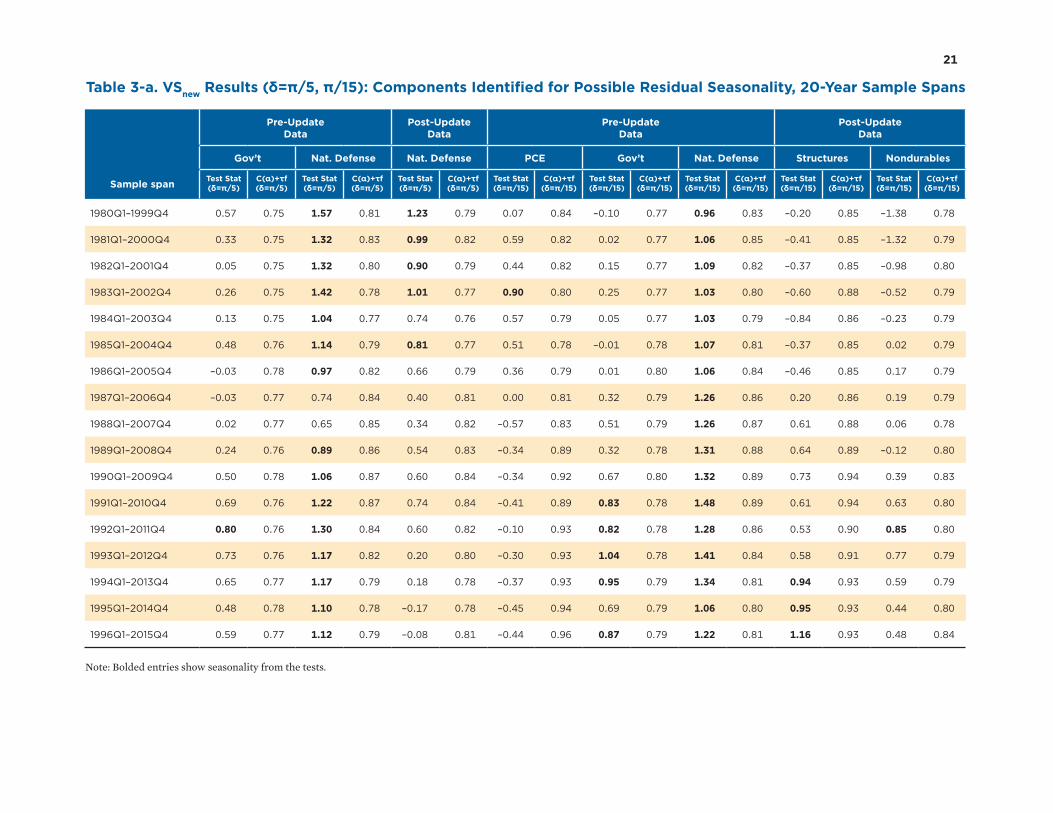
then the null hypothesis of no spectral peak is rejected. Table 3-a below shows the NIPA aggregates

from both pre- and post-comprehensive updated data for which the null hypothesis of the VS test

is rejected in the 20-year sample spans. Using the pre-comprehensive updated data in the test and

setting 𝛿 = 𝜋/5, the null hypothesis is rejected in the 1992Q1–2011Q4 sample span of government

expenditure and in 15 out of 17 sample spans of national defense. After the comprehensive update,

20

no spectral peak is detected in government expenditure, and for national defense the number of

sample spans for which the null hypothesis is rejected reduces from 15 to 5.

Setting the nearest neighbors at a closer distance from the seasonal frequency of interest, 𝛿 = 𝜋/15 ,

the VS test results using data before the comprehensive update show possible presence of dynamic

residual seasonality in the 1983Q1–2002Q2 sample span of PCE, 5 sample spans of government

expenditure from 1991Q1–2015Q4, and all 17 sample spans of national defense. After the compre-

hensive updates, the VS tests show no residual seasonality in PCE, government expenditure and

national defense. However, the null hypothesis is rejected in 3 sample spans of structures and 1

sample span of nondurables.

The VS test is also conducted using the 15-year sample spans. Using data before the comprehensive

update and setting 𝛿 = 𝜋/5, the null hypothesis of no spectral peak is rejected in the 1999Q1–2013Q4

sample span of nondurables, in 3 sample spans of government expenditure including the 2 most

recent sample spans, and in 11 out of the 22 sample spans of national defense. Using data after the

comprehensive update, the null hypothesis is rejected in only 1 sample span of national defense.

Setting 𝛿 = 𝜋/15, the null hypothesis is rejected in 2 sample spans of nondurables, in the most

recent 4 sample spans of government expenditure, 14 sample spans of national defense since

1986Q1, and the 2001Q1–2015Q4 sample span of state and local government using data before the

comprehensive update; and the null hypothesis is rejected in only 1 sample span of structures using

data after the comprehensive update.

Three general observations stand out from the VS test results: 1) for a given 𝛿, which defines the

tightness of the peak detection region in the frequency spectrum, the null hypothesis is rejected in

fewer NIPA components and fewer sample spans in the post-comprehensive updated data, using

both 20- and 15-year sample spans; 2) spectral peaks detected in the wider test region (𝛿 = 𝜋/5)

may not be present in the narrower test region (𝛿 = 𝜋/15) and vice versa; and 3) spectral peaks are

detected in some NIPA components (for example, government expenditure, national defense, and

structures) using both 20- and 15-year sample spans but not necessarily in the same time periods.

For example, for 𝛿 = 𝜋/15, a spectral peak is detected in some of the 20- and 15-year sample spans in

national defense in the pre-comprehensive updated data. However, if the 20-year sample spans are

used, a peak is detected in the 1980Q1–1999Q4 sample span, whereas if the 15-year sample spans

are used, no spectral peak is detected in the 4 sample spans from 1980Q1 to 1999Q4.

21

Table 3-a. VSnew Results (δ=π/5, π/15): Components Identified for Possible Residual Seasonality, 20-Year Sample Spans

Sample span

Pre-Update Data

Post-Update Data

Pre-Update Data

Post-Update Data

Gov’t Nat. Defense Nat. Defense PCE Gov’t Nat. Defense Structures Nondurables

Test Stat(δ=π/5)

C(α)+τf(δ=π/5)

Test Stat(δ=π/5)

C(α)+τf(δ=π/5)

Test Stat(δ=π/5)

C(α)+τf(δ=π/5)

Test Stat(δ=π/15)

C(α)+τf(δ=π/15)

Test Stat(δ=π/15)

C(α)+τf(δ=π/15)

Test Stat(δ=π/15)

C(α)+τf(δ=π/15)

Test Stat(δ=π/15)

C(α)+τf(δ=π/15)

Test Stat(δ=π/15)

C(α)+τf(δ=π/15)

1980Q1–1999Q4 0.57 0.75 1.57 0.81 1.23 0.79 0.07 0.84 –0.10 0.77 0.96 0.83 –0.20 0.85 –1.38 0.78

1981Q1–2000Q4 0.33 0.75 1.32 0.83 0.99 0.82 0.59 0.82 0.02 0.77 1.06 0.85 –0.41 0.85 –1.32 0.79

1982Q1–2001Q4 0.05 0.75 1.32 0.80 0.90 0.79 0.44 0.82 0.15 0.77 1.09 0.82 –0.37 0.85 –0.98 0.80

1983Q1–2002Q4 0.26 0.75 1.42 0.78 1.01 0.77 0.90 0.80 0.25 0.77 1.03 0.80 –0.60 0.88 –0.52 0.79

1984Q1–2003Q4 0.13 0.75 1.04 0.77 0.74 0.76 0.57 0.79 0.05 0.77 1.03 0.79 –0.84 0.86 –0.23 0.79

1985Q1–2004Q4 0.48 0.76 1.14 0.79 0.81 0.77 0.51 0.78 –0.01 0.78 1.07 0.81 –0.37 0.85 0.02 0.79

1986Q1–2005Q4 –0.03 0.78 0.97 0.82 0.66 0.79 0.36 0.79 0.01 0.80 1.06 0.84 –0.46 0.85 0.17 0.79

1987Q1–2006Q4 –0.03 0.77 0.74 0.84 0.40 0.81 0.00 0.81 0.32 0.79 1.26 0.86 0.20 0.86 0.19 0.79

1988Q1–2007Q4 0.02 0.77 0.65 0.85 0.34 0.82 –0.57 0.83 0.51 0.79 1.26 0.87 0.61 0.88 0.06 0.78

1989Q1–2008Q4 0.24 0.76 0.89 0.86 0.54 0.83 –0.34 0.89 0.32 0.78 1.31 0.88 0.64 0.89 –0.12 0.80

1990Q1–2009Q4 0.50 0.78 1.06 0.87 0.60 0.84 –0.34 0.92 0.67 0.80 1.32 0.89 0.73 0.94 0.39 0.83

1991Q1–2010Q4 0.69 0.76 1.22 0.87 0.74 0.84 –0.41 0.89 0.83 0.78 1.48 0.89 0.61 0.94 0.63 0.80

1992Q1–2011Q4 0.80 0.76 1.30 0.84 0.60 0.82 –0.10 0.93 0.82 0.78 1.28 0.86 0.53 0.90 0.85 0.80

1993Q1–2012Q4 0.73 0.76 1.17 0.82 0.20 0.80 –0.30 0.93 1.04 0.78 1.41 0.84 0.58 0.91 0.77 0.79

1994Q1–2013Q4 0.65 0.77 1.17 0.79 0.18 0.78 –0.37 0.93 0.95 0.79 1.34 0.81 0.94 0.93 0.59 0.79

1995Q1–2014Q4 0.48 0.78 1.10 0.78 –0.17 0.78 –0.45 0.94 0.69 0.79 1.06 0.80 0.95 0.93 0.44 0.80

1996Q1–2015Q4 0.59 0.77 1.12 0.79 –0.08 0.81 –0.44 0.96 0.87 0.79 1.22 0.81 1.16 0.93 0.48 0.84

Note: Bolded entries show seasonality from the tests.

22

Table 3-b. VSnew Results (δ=π/5, π/15): Components Identified with Possible Residual Seasonality, 15-Year Sample Spans

Sample span

Pre-Update Data

Post-Update Data

Pre-Update Data

Post-Update Data

NonDurables Gov’t Nat. Defense Nat. Defense Nondurables Gov’t Nat. Defense State & Local Structures

Test Stat(δ=π/5)

C(α)+τf(δ=π/5)

Test Stat(δ=π/5)

C(α)+τf(δ=π/5)

Test Stat(δ=π/5)

C(α)+τf(δ=π/5)

Test Stat(δ=π/5)

C(α)+τf(δ=π/5)

Test Stat(δ=π/15)

C(α)+τf(δ=π/15)

Test Stat(δ=π/15)

C(α)+τf(δ=π/15)

Test Stat(δ=π/15)

C(α)+τf(δ=π/15)

Test Stat(δ=π/15)

C(α)+τf(δ=π/15)

Test Stat(δ=π/15)

C(α)+τf(δ=π/15)

1980Q1–1994Q4 –0.98 0.76 0.09 0.75 0.43 0.81 0.27 0.83 –1.51 0.77 –0.46 0.75 0.22 0.82 –0.72 0.85 –0.33 0.85

1981Q1–1995Q4 –1.16 0.76 –0.07 0.77 0.56 0.86 0.42 0.88 –1.60 0.76 –0.33 0.77 0.12 0.86 –0.88 0.86 -0.56 0.85

1982Q1–1996Q4 –1.13 0.75 0.12 0.78 0.88 0.83 0.63 0.86 –1.49 0.75 –0.05 0.78 0.03 0.83 –0.82 0.81 –0.83 0.87

1983Q1–1997Q4 –0.85 0.75 0.38 0.77 0.72 0.83 0.47 0.85 –0.95 0.76 0.20 0.77 0.29 0.83 –0.66 0.79 –0.94 0.85

1984Q1–1998Q4 –0.70 0.76 0.69 0.75 1.18 0.83 1.00 0.85 –0.72 0.76 0.07 0.75 0.83 0.83 –0.35 0.82 –1.57 0.80

1985Q1–1999Q4 –1.54 0.76 0.93 0.76 1.43 0.83 1.15 0.85 –0.84 0.77 –0.11 0.76 0.72 0.83 –0.45 0.81 –1.13 0.78

1986Q1–2000Q4 –1.75 0.81 0.21 0.80 1.04 0.88 0.76 0.90 –0.75 0.81 0.02 0.80 0.89 0.88 –0.60 0.81 –1.04 0.79

1987Q1–2001Q4 –1.30 0.78 0.02 0.78 1.07 0.88 0.69 0.91 –0.38 0.78 0.11 0.78 1.00 0.88 –0.38 0.77 –0.10 0.79

1988Q1–2002Q4 –1.15 0.77 0.13 0.77 1.13 0.85 0.72 0.87 –0.07 0.77 0.02 0.77 0.93 0.85 –0.90 0.75 0.08 0.87

1989Q1–2003Q4 –0.85 0.77 0.05 0.77 1.01 0.86 0.78 0.87 0.07 0.78 0.03 0.78 0.90 0.86 –1.06 0.79 0.13 0.87

1990Q1–2004Q4 –0.67 0.78 0.31 0.79 1.07 0.89 0.75 0.90 0.55 0.78 0.37 0.79 1.04 0.89 –0.96 0.80 0.59 0.88

1991Q1–2005Q4 –0.72 0.80 0.35 0.77 1.19 0.92 0.93 0.93 0.59 0.80 0.60 0.78 1.18 0.92 –0.65 0.81 0.24 0.85

1992Q1–2006Q4 –0.07 0.81 0.28 0.77 0.88 0.89 0.56 0.91 0.87 0.81 0.50 0.78 1.09 0.90 –0.44 0.81 0.53 0.85

1993Q1–2007Q4 –0.05 0.80 0.07 0.78 0.55 0.89 0.16 0.92 0.83 0.80 0.67 0.78 1.16 0.89 –0.26 0.79 0.49 0.87

1994Q1–2008Q4 –0.19 0.78 0.04 0.78 0.64 0.89 0.19 0.91 0.01 0.78 0.44 0.78 0.90 0.89 –0.34 0.78 0.55 0.92

1995Q1–2009Q4 –0.36 0.76 –0.14 0.77 0.61 0.89 –0.13 0.89 0.29 0.76 0.16 0.77 0.60 0.89 –0.41 0.79 0.60 0.97

1996Q1–2010Q4 –0.02 0.75 0.09 0.78 0.75 0.88 0.01 0.88 0.36 0.76 0.49 0.78 0.88 0.88 –0.12 0.79 0.49 0.96

1997Q1–2011Q4 0.10 0.76 0.33 0.75 0.80 0.85 –0.20 0.86 0.55 0.76 0.55 0.75 1.00 0.85 –0.29 0.80 0.54 0.92

1998Q1–2012Q4 0.18 0.76 0.27 0.75 0.71 0.82 –0.70 0.84 0.33 0.76 0.86 0.75 1.10 0.82 –0.27 0.79 0.65 0.95

1999Q1–2013Q4 0.77 0.76 0.55 0.75 0.59 0.82 –1.11 0.85 0.39 0.76 1.01 0.76 1.12 0.82 0.23 0.80 0.85 0.94

2000Q1–2014Q4 0.10 0.81 1.29 0.79 1.16 0.79 0.25 0.81 -0.02 0.81 1.21 0.79 1.63 0.80 0.52 0.82 0.73 0.93

2001Q1–2015Q4 0.41 0.83 1.34 0.81 1.35 0.82 0.11 0.83 0.32 0.83 1.58 0.82 1.54 0.83 0.95 0.88 1.01 0.94

Note: Bolded entries show seasonality from the tests.

23

4.3 Results from the ROOT Diagnostic for Detecting Dynamic Seasonality

The ROOT diagnostic examines oscillatory effects in the autocovariance sequence of frequency

𝜃 = 𝜋/2. The persistence 𝜌 ∈ (0, 1) corresponds to the degree of dynamic seasonality that is pres-

ent. The null hypothesis states that for a given frequency 𝜃 there is seasonality of degree 𝜌 present.

Hence, low p-values indicate the absence of seasonality (of a given degree of persistency), whereas

for VS the opposite is true: a low p-value indicates that seasonality is indeed present. For the ROOT

test, we consider a range of 𝜌 and report which of the corresponding p-values are greater than our

chosen threshold 𝛼—these are the values of 𝜌 for which we fail to reject the null hypothesis, that is,

there is evidence of the presence of seasonality of degree 𝜌.

In our testing, the null hypothesis is set so that seasonality of degree 𝜌 can be rejected at a signifi-

cance level of 𝛼 = .10 for all 𝜌 ∈ (0.98, 1). The value of 𝜌 = .98 corresponds to a substantial degree of

oscillation in the autocorrelation function; lowering this value requires weaker forms of seasonality

to be screened out. We consider a grid of values for 𝜌 ∈ (0.98, 1), and record the p-value for each

null hypothesis. Then for each series and span, we record both the maximum of these p-values and

the p-value for the case of 𝜌 = .999, as this case may be of special interest (as it corresponds to the

most persistent form of stable seasonality for this range of 𝜌). Note that if all these p-values are less

than 𝛼 = .10 (or, equivalently, the maximum is less than 𝛼 = .10), then the presence of seasonality is

rejected; conversely, when the maximum p- value exceeds .10, then seasonality is not rejected for at

least one value of 𝜌 ∈ (0.98, 1).

Table 4-a below shows that using the 20-year sample spans, the ROOT diagnostic tests found no

identifiable presence of residual seasonality due to persistent seasonal roots in the autoregressive

polynomials of real GDP and 18 major components in the pre-comprehensive updated data. The

only exception is national defense, for which the ROOT diagnostic test shows a possible presence

of residual seasonality in 4 out of the 17 sample spans from 1992Q1 to 2015Q4.

Table 4-b shows that using the 15-year sample spans, the ROOT diagnostic test found identifiable

presence of residual seasonality in 5 sample spans of national defense from 1996Q1–2015Q4 and in

the 2001Q1–2015Q4 sample span of government expenditure in the pre-comprehensive updated

data. No identifiable presence of residual seasonality is found in real GDP and the other compo-

nents both before and after the comprehensive update.

24

Table 4-a. ROOT Diagnostic Test Results Using Data before and after Comprehensive Update: 20-Year Sample Spans

Sample span

Pre-Update Data Post-Update Data

Gov’t Nat. Defense Gov’t Nat. Defense

Max p-value ρ=0.999

Max p-value ρ=0.999

Max p-value ρ=0.999

Max p-value ρ=0.999

1980Q1–1999Q4 0.00 0.00 0.00 0.00 0.00 0.00 0.00 0.00

1981Q1–2000Q4 0.00 0.00 0.01 0.01 0.00 0.00 0.00 0.00

1982Q1–2001Q4 0.00 0.00 0.01 0.01 0.00 0.00 0.00 0.00

1983Q1–2002Q4 0.00 0.00 0.01 0.00 0.00 0.00 0.00 0.00

1984Q1–2003Q4 0.00 0.00 0.01 0.00 0.00 0.00 0.00 0.00

1985Q1–2004Q4 0.00 0.00 0.01 0.01 0.00 0.00 0.00 0.00

1986Q1–2005Q4 0.00 0.00 0.00 0.00 0.00 0.00 0.00 0.00

1987Q1–2006Q4 0.00 0.00 0.01 0.01 0.00 0.00 0.00 0.00

1988Q1–2007Q4 0.00 0.00 0.01 0.00 0.00 0.00 0.00 0.00

1989Q1–2008Q4 0.00 0.00 0.02 0.01 0.00 0.00 0.00 0.00

1990Q1–2009Q4 0.00 0.00 0.04 0.02 0.00 0.00 0.00 0.00

1991Q1–2010Q4 0.01 0.00 0.08 0.03 0.00 0.00 0.00 0.00

1992Q1–2011Q4 0.01 0.00 0.17 0.07 0.00 0.00 0.00 0.00

1993Q1–2012Q4 0.01 0.00 0.09 0.04 0.00 0.00 0.00 0.00

1994Q1–2013Q4 0.01 0.00 0.13 0.05 0.00 0.00 0.00 0.00

1995Q1–2014Q4 0.01 0.00 0.10 0.05 0.00 0.00 0.00 0.00

1996Q1–2015Q4 0.01 0.00 0.17 0.07 0.00 0.00 0.01 0.00

Note: Bolded entries show seasonality from the tests.

25

Table 4-b. ROOT Diagnostic Test Results Using Data before and after Comprehensive Update: 15-Year Sample Spans

Sample span

Pre-Update Data Post-Update Data

Gov’t Nat. Defense Gov’t Nat. Defense

Max p-value ρ=0.999

Max p-value ρ=0.999

Max p-value ρ=0.999

Max p-value ρ=0.999

1980Q1–1994Q4 0.00 0.00 0.02 0.01 0.00 0.00 0.00 0.00

1981Q1–1995Q4 0.00 0.00 0.00 0.00 0.00 0.00 0.00 0.00

1982Q1–1996Q4 0.00 0.00 0.00 0.00 0.00 0.00 0.00 0.00

1983Q1–1997Q4 0.00 0.00 0.01 0.01 0.00 0.00 0.00 0.00

1984Q1–1998Q4 0.00 0.00 0.04 0.02 0.00 0.00 0.00 0.00

1985Q1–1999Q4 0.00 0.00 0.01 0.00 0.00 0.00 0.00 0.00

1986Q1–2000Q4 0.00 0.00 0.02 0.01 0.00 0.00 0.00 0.00

1987Q1–2001Q4 0.00 0.00 0.00 0.00 0.00 0.00 0.00 0.00

1988Q1–2002Q4 0.00 0.00 0.02 0.01 0.00 0.00 0.00 0.00

1989Q1–2003Q4 0.00 0.00 0.04 0.02 0.00 0.00 0.00 0.00

1990Q1–2004Q4 0.00 0.00 0.03 0.01 0.00 0.00 0.00 0.00

1991Q1–2005Q4 0.00 0.00 0.07 0.03 0.00 0.00 0.00 0.00

1992Q1–2006Q4 0.00 0.00 0.04 0.02 0.00 0.00 0.00 0.00

1993Q1–2007Q4 0.00 0.00 0.03 0.02 0.00 0.00 0.00 0.00

1994Q1–2008Q4 0.00 0.00 0.02 0.01 0.00 0.00 0.00 0.00

1995Q1–2009Q4 0.00 0.00 0.05 0.03 0.00 0.00 0.00 0.00

1996Q1–2010Q4 0.00 0.00 0.44 0.19 0.00 0.00 0.00 0.00

1997Q1–2011Q4 0.00 0.00 0.41 0.18 0.00 0.00 0.00 0.00

1998Q1–2012Q4 0.00 0.00 0.02 0.01 0.00 0.00 0.00 0.00

1999Q1–2013Q4 0.00 0.00 0.20 0.10 0.00 0.00 0.00 0.00

2000Q1–2014Q4 0.00 0.00 0.57 0.25 0.00 0.00 0.00 0.00

2001Q1–2015Q4 0.42 0.19 0.59 0.25 0.00 0.00 0.00 0.00

Note: Bolded entries show seasonality from the tests.

26

4.4 Discussion of Results from the Proposed Diagnostic Tests

There are four major observations to note from the results of the three diagnostic tests. First, using

the same sample size in the test, the three diagnostic tests do not always identify a possible pres-

ence of residual seasonality in the same NIPA aggregates or in the same sample spans. For example,

the MBF test identifies the possible presence of residual seasonality in real GDP in a few sample

spans and in some sample spans of several NIPA aggregates such as GDPI, services, residential

investment, exports, imports, and the three price indexes, but no residual seasonality is identified

in these components from the VS and ROOT diagnostic tests. The explanation for the differential

results from the three tests is that the three diagnostics are designed for detecting different types of

seasonality. The MBF test is intended to test for stable seasonality, whereas the VS and ROOT diag-

nostics are designed to test for dynamic seasonality, respectively, in the frequency and time domain.

Some NIPA aggregates may only exhibit stable residual seasonality but not dynamic seasonality.

Others, such as PCE, nondurables, structures, and state and local government, may exhibit dynamic

seasonality in the frequency domain but not in the time domain. There are even some aggregates,

such as government and national defense, that may exhibit residual seasonality of all three types

in some sample spans. Moreover, results for the VS and ROOT tests depend upon user-defined set-

tings, such as 𝛿, 𝜏, choice of taper, choice of bandwidth, range of 𝜌, and model selection criteria.

Second, the possible presence of fixed residual seasonality is identified in around 50 percent of the

NIPA aggregates being tested at least in some sample spans in the pre- and/or post-comprehen-

sive updated estimates, whereas dynamic seasonality in the frequency domain is identified in just a

few NIPA aggregates, mostly in the estimates before the comprehensive update. Dynamic season-

ality in the time domain is identified only in two components, national defense and government,

in the pre-comprehensive updated estimates. Since stable seasonality is typically only present in

raw data, one may ask why fixed seasonality is detected in the seasonally adjusted data. This could

be because real GDP and NIPA aggregates are indirectly seasonally adjusted; stable seasonality

that may not be identifiable in the detailed component series may become identifiable through the

aggregation of detailed seasonally adjusted series. This observation underscores the importance

of detecting and correcting stable and dynamic residual seasonality while aggregating seasonally

adjusted detailed series.

Third, results using the 20- and 15-year sample spans may not identify residual seasonality in the

same NIPA components or in the sample time periods. For example, the MBF test identifies the

possible presence of stable seasonality in durables, intellectual property, imports, nondefense, and

nominal GDP only from the 15-year sample spans and not from the 20-year sample spans. Using the

20-year sample spans, the MBF test identifies stable residual seasonality in the post-comprehensive

update of real GDP during the 1992Q1–2012Q4 periods, whereas when using the 15-year sample

27

spans from the same vintage of data, stable residual seasonality is identified in real GDP only in the

1987Q1–2001Q4 sample span. Moreover, the VS test (with 𝛿 = 𝜋/5) identifies the possible presence

of dynamic seasonality in national defense during the 1980Q1–2004Q4 periods using the 20-year

sample spans from the post-comprehensive updated data, whereas using the 15-year sample spans,

dynamic seasonality is only identified in the 1985Q1–1999Q4 sample span. It frequently occurs that

seasonality diagnostics may produce different results when different sample spans are used. This

study chooses 20- and 15-year sample spans for testing, with the consideration that these sample

spans are long enough to cover business cycles of various lengths, and that the sample size is large

enough to properly estimate test statistics.

Fourth, our test results demonstrate improvements in seasonal adjustment in the U.S. national

accounts after the most recent comprehensive update. Fewer NIPA aggregates are identified with

the possible presence of residual seasonality from the MBF test using the 20-year sample spans

and from the VS and ROOT tests using both 20- and 15-year sample spans. The possible presence

of residual seasonality is also identified in fewer sample spans after the comprehensive update.

Particularly, government and national defense are the two NIPA aggregates for which both sta-

ble seasonality and spectral peaks are identified in most sample spans before the comprehensive

update, whereas after the comprehensive update, residual seasonality is identified in only a few

sample spans.

28

5. Further Research and Concluding Remarks

In this study, we have reviewed several critiques of residual seasonality in real GDP and its major

components published in the U.S. national accounts. We have identified appropriate diagnostics

from available tests that have been vetted and published, and evaluated the methods used in the cri-

tiques. We have applied our own analysis with appropriate diagnostics, focusing on tests for season-

ally adjusted data, looking at stable and dynamic seasonality. We tested for stable and dynamic sea-

sonality in real GDP and in 19 NIPA aggregates from 1980Q1 to 2015Q4 using data from before and

after the 2018 comprehensive update. Because seasonality diagnostics can be sensitive to the sample

spans used in the tests, we compared the test results using both 20- and 15-year sample spans.

Using data after the comprehensive update, possible residual seasonality is identified in real GDP

in four recent 20-year sample spans from the MBF test but not in the 15-year sample spans; pos-

sible residual seasonality is also identified from the MBF test in eight NIPA aggregates in some

20-year sample spans and in 15 NIPA aggregates in some 15-year sample spans. Dynamic seasonal-

ity is identified in four components from the VS test and in two components from the ROOT tests.

We have observed from our analysis that: 1) more components are identified with possible residual

seasonality from the MBF test than from the VS and ROOT diagnostic tests; 2) because the diagnos-

tics are intended to test for different types of residual seasonality, the three diagnostics do not always

identify residual seasonality in the same components or in the same sample spans; 3) for a given

diagnostic test using the 20- and 15-year sample spans, residual seasonality may not always be iden-

tified in the same NIPA components or in the same time periods; and 4) residual seasonality is iden-

tified in fewer components and fewer sample spans in real GDP and NIPA aggregates after the com-

prehensive update, reflecting improvements in seasonal adjustment in the U.S. national accounts.

The results from this study show that the three diagnostic tests presented here could be useful

tools for detecting residual seasonality in the national accounts estimates. Future research will

focus on developing a method for further mitigating residual seasonality. Quarterly seasonal adjust-

ments in official statistics are often not the result of a direct adjustment of the quarterly series, but

instead are an indirect adjustment arising from the aggregation of the seasonally adjusted monthly

series. However, temporal aggregation of seasonal adjusted monthly series to a quarterly frequency

can exhibit seasonality. The residual seasonality detected in the quarterly series in this study could

have arisen from temporal aggregation of the seasonally adjusted monthly series.

An implementable solution method is being built on prior work that uses a benchmarking and rec-

onciliation framework to enforce seasonal adjustment adequacy as temporal aggregation is applied,

where adequacy is metrized and supplied as a hard constraint to the benchmarking optimization

29

problem (McElroy 2018, McElroy et al. 2019). This proposed solution method involves nonlinear

optimization for each series, whereby monthly adjustments are changed as little as possible, such that

they are still adequate and aggregated to the quarterly adjustment, which is also enforced to be ade-

quate. Any of the three diagnostic tests presented in this study could be utilized in tandem with the

benchmarking and reconciliation procedure. The outlined solution method could be applied to the

national accounts estimates to correct residual seasonality that has arisen from temporal aggregation.

30

References

Blakely, C. and T.S. McElroy. 2017. “Signal Extraction Goodness-of-fit Diagnostic Tests Under

Model Parameter Uncertainty: Formulations and Empirical Evaluation,” Econometric Reviews 36, 4

(April): 447–467.

Canova, F. and B.E. Hansen. 1995. “Are Seasonal Patterns Constant over Time? A Test for Seasonal

Stability,” Journal of Business and Economic Statistics 13 (July): 237–252.

Cowan, B., S. Smith, and S. Thompson. 2018. “Seasonal Adjustment in the National Income and

Product Accounts,” Survey of Current Business 98 (August): 1–14.

Findley, D.F., D.P. Lytras, and T.S. McElroy. 2017. Detecting Seasonality in Seasonally Adjusted Monthly

Time Series. Census Bureau Research Report 2017-03. Washington , D.C.: Census Bureau, February.

https://www.census.gov/content/dam/Census/library/working-papers/2017/adrm/rrs2017-03.pdf

Findley, D.F., B.C. Monsell, W.R. Bell, M.C. Otto, and B.C. Chen. 1998”New Capabilities and

Methods of the X-12-ARIMA Seasonal Adjustment Program,” Journal of Business and Economic

Statistics 16 (April): 127–177.

Franses, P.H. 1994. “A Multivariate Approach to Modeling Univariate Seasonal Time Series,”

Journal of Econometrics 63 (July): 133–151.

Friedman, M. 1937. “The Use of Ranks to Avoid the Assumption of Normality Implicit in the

Analysis of Variance,” Journal of the American Statistical Association 32, no. 200, 675–701.

Furman, J. “Second Estimate of GDP for the First Quarter of 2015,” Council of Economic Advisers

(Blog), The White House, May 29, 2015. https://obamawhitehouse.archives.gov/blog/2015/05/29/

second-estimate-gdp-first-quarter-2015

Gilbert, C.E., N.J. Morin, A.O. Paciorek, and C.R. Sahm. 2015. “Residual Seasonality in GDP,” FEDS

Notes. Washington: Board of Governors of the Federal Reserve System, May 14, 2015. https://doi.

org/10.17016/2380-7172.1538

Gómez, V. and A. Maravall. 1996. “Programs TRAMO and SEATS. Instructions for the User,”

Working Paper 9628, Servicio de Estudios, Banco de España.

Groen, J. and P. Russo. “The Myth of First-Quarter Residual Seasonality,” Liberty Street Economics

(Blog), The Federal Reserve Bank of New York, June 8, 2015.

31

Hylleberg, S., R.F. Engle, C.W.J. Granger, and B.S. Yoo. 1990. “Seasonal Integration and

Cointegration,” Journal of Econometrics 44, 215–238.

Kruskal, W.H. and W.A. Wallis. 1952. “Use of Ranks in One-Criterion Variance Analysis,” Journal of

the American Statistical Association 47, 583–621.

Lengermann, P., E. Morin, A. Paciorek, E. Pinto, and C. Sahm. 2017. “Another Look at Residual

Seasonality in GDP,” FEDS Notes. Washington: Board of Governors of the Federal Reserve System.

https://doi.org/10.17016/2380-7172.2031

Lothian, J. and M. Morry. 1978. “A Set of Quality Control Statistics for the X-11 ARIMA Seasonal

Adjustment Method,” Working Paper 78-10-005E, Methodology Branch, Statistics Canada, Ottawa,

ON, Canada.

Lunsford, K.G. 2017. “Lingering Residual Seasonality in GDP Growth,” Economic Commentary,

Federal Reserve Bank of Cleveland, March 28, 2017.

Lytras, D.P., R.M. Feldpausch, and W.R. Bell. 2007. “Determining Seasonality: A Comparison

of Diagnostics from X-12-ARlMA.” In Proceedings of the Third International Conference on

Establishment Surveys (ICES-III), Montreal, Canada. https://www.census.gov/content/damq/

Census/library/working-papers/2007/adrm/ices2007dpl.pdf

Maravall, A. 2012. “Update of Seasonality Tests and Automatic Model Identification in TRAMO-

SEATS,” Banco de España (November 2012 draft).

McCulla, S.H. and S. Smith. 2015. “Preview of the 2015 Annual Revision of the National Income and

Product Accounts,” Survey of Current Business 95 (June):1–8.

McElroy, T.S. 2012. “An Alternative Model-Based Seasonal Adjustment that Reduces Over-

Adjustment,” Taiwan Economic Forecast and Policy 43, 33–70.

McElroy, T.S. 2018. “Seasonal Adjustment Subject to Accounting Constraints,” Statistica

Neerlandica 72, 574–589.

McElroy, T.S. 2021. “A Diagnostic for Seasonality Based Upon Polynomial Roots of ARMA Models,”

Journal of Official Statistics, forthcoming.

McElroy, T.S. and S. Holan. 2009. “A Nonparametric Test for Residual Seasonality,” Survey

Methodology 35, no. 1, 67–83.

32

McElroy, T.S., O. Pang, and B. Monsell. 2019. “Seasonal Adjustment Subject to Lower Frequency

Benchmarks,” In the 2019 Proceedings of American Statistical Association: Alexandria, VA.

McElroy, T.S. and D.N. Politis. 2020. Time Series: A First Course with Bootstrap Sampler. New York:

Chapman & Hall.

McElroy, T.S. and A. Roy. 2021. “Testing for Adequacy of Seasonal Adjustment in the Frequency

Domain,” Journal of Statistical Planning and Inference 221, 241–255.

Moulton, B.R. and B.D. Cowan. 2016. “Residual Seasonality in GDP and GDI: Findings and Next

Steps,” Survey of Current Business 96 (July): 1–6.

Müller, U.K. and M.W. Watson 2008. “Testing Models of Low-Frequency Variability,” Econometrica

76, no. 5, 979-1016.

Müller, U.K. and M.W. Watson 2015. “Low-Frequency Econometrics,” National Bureau of Economic

Research Working Paper Series 21564, (September): 1-45, http://www.nber.org/papers/w21564

Nyblom, J. 1989. “Testing for the Constancy of Parameters Over Time,” Journal of the American

Statistical Association 84, no. 405, 223-230.

Peneva, E. 2014. “Residual Seasonality in Core Consumption Price Inflation,” FEDS Notes.

Washington: Board of Governors of the Federal Reserve System, October 14, 2014. https://doi.

org/10.17016/2380-7172.0030

Phillips, K. and J. Wang. 2016. “Residual Seasonality in U.S. GDP Data” FRB of Dallas Working

Paper No. 1608. Available at SSRN: https://ssrn.com/abstract=2866843 or at http://dx.doi.org/

10.24149/wp1608

Priestley, M.B. 1981. Spectral Analysis and Time Series. New York: Academic Press.

Rudebusch, G.D., D. Wilson, and T. Mahedy. 2015. “The Puzzle of Weak First-Quarter GDP

Growth,” Federal Reserve Bank of San Francisco Economic Letter, May 18, 2015.

Somsuk, N. 2019. “Taking a Closer Look at Residual Seasonality and U.S. GDP Growth,” in On the

Economy, Federal Reserve Bank of St. Louis, January 2019.

Soukup, R. and D. Findley. 1999. “On the spectrum diagnostics used by X-12-ARIMA to indicate the

presence of trading day effects after modeling or adjustment.” In the 1999 Proceedings of American

33

Statistical Association: Alexandria, VA, and available at https://www.census.gov/content/dam/

Census/library/working-papers/1999/adrm/rr9903s.pdf

Stark, T. 2015. “First Quarter in the National Income and Product Accounts,” in Research Rap,

Federal Reserve Bank of Philadelphia, May 14, 2015.

U.S. Census Bureau. 2020. “X-13ARIMA-SEATS Reference Manual,”, Washington D.C.: U.S. Census

Bureau, available from https://www2.census.gov/software/x-13arima-seats/x13as/windows/docu-

mentation/docx13ashtml.pdf

Wright, J. H. 2018. “Seasonal Adjustment of NIPA Data,” NBER Working Paper 24895, August 2018.