appropriateness of some resampling-based inference

Appropriateness of some resampling-based inference procedures for

assessing performance of prognostic classifiers derived from microarray

data

Lara Lusa1,2, Lisa M. McShane3,*, Michael D. Radmacher4, Joanna H. Shih3, George W.

Wright3, and Richard Simon3

1Department of Experimental Oncology, Istituto Nazionale per lo Studio e la Cura dei

Tumori, Milano, Italy

2Molecular Cancer Genetics Group, Fondazione Istituto FIRC di Oncologia Molecolare

(IFOM), Milano, Italy

3Biometric Research Branch, National Cancer Institute, Bethesda, MD 20892-7434,

U.S.A.

4Center for Biostatistics, The Ohio State University, Columbus, OH 43210

*Correspondence to: Lisa M. McShane

Biometric Research Branch, EPN 8126

National Cancer Institute

6130 Executive Blvd.

Bethesda, MD 20892-7434

Email: [email protected]

Phone: 301-402-0636

Fax: 301-402-0560

1

Summary

The goal of many gene-expression microarray profiling clinical studies is to develop a

multivariate classifier to predict patient disease outcome from a gene expression profile

measured on some biological specimen from the patient. Often some preliminary

validation of the predictive power of a profile-based classifier is carried out using the

same data set that was used to derive the classifier. Techniques such as cross-validation

or bootstrapping can be used in this setting to assess predictive power, and if applied

correctly, can result in a less biased estimate of predictive accuracy of a classifier.

However, some investigators have attempted to apply standard statistical inference

procedures to assess the statistical significance of associations between true and cross-

validated predicted outcomes. We demonstrate in this paper that naïve application of

standard statistical inference procedures to these measures of association can result in

greatly inflated testing type I error rates and confidence intervals with poor coverage

probabilities. Our results suggest that some of the claims of exceptional prognostic

classifier performance that have been reported in prominent biomedical journals in the

past few years should be interpreted with great caution.

Key words: cross-validation, microarray, gene expression, classification, resampling,

molecular profiling

2

1. Introduction

A frequent goal in gene expression microarray clinical studies is to develop a multivariate

classifier of disease outcome [1-9]. In these studies, gene expression microarray assays

are performed on tissue or other biological material from patients for whom clinical

outcomes such as survival are known. The results of the microarray assays are thousands

of gene expression measures, comprising a “profile”, for each of the patient samples

assayed. Mathematical methods are applied to the expression profile data to develop a

multivariate classifier to predict disease outcome. For example, van’t Veer et al. [1]

conducted gene expression microarray analyses on breast tumors and used the data from

78 of the lymph node-negative tumors to build a 70-gene classifier of clinical outcome;

they reported it had excellent ability to distinguish between breast cancer patients who

did versus did not develop distant metastases within 5 years. Beer et al. [3] developed a

50-gene risk index using gene expression profiles from 86 primary lung adenocarcinomas

and demonstrated that their risk index could separate patients into subgroups with distinct

overall survival probabilities.

An important question is how one can reliably assess the performance of

microarray-based classifiers. For example, suppose that patient outcomes are classified

as “good prognosis” (long survival) versus “poor prognosis” (short survival). A common

approach to assessing the performance of a multivariate classifier is to estimate its

prediction accuracy, defined as the proportion of samples it correctly classifies. Ideally,

this assessment of the classifier would be carried out on a completely independent set of

patient specimens, but rarely are there readily available sufficiently large numbers of

specimens that are amenable to microarray analysis and accompanied by the necessary

3

clinical information. The alternative is to estimate prediction accuracy using the same

data from which the classifier was derived. However, when re-using the same data,

proper application of resampling methods such as cross-validation [10] or bootstrapping

[11-12] is essential in order to avoid seriously overestimating the prediction accuracy.

As an alternative to, or in addition to, estimating the proportion of correct

classifications, some authors have chosen to estimate the association of the true (known)

classes with the classes predicted from the cross-validated classifier and to perform a test

of the statistical significance of that association. For example, this is an approach that

was taken in the study by van’t Veer et al. [1] that has received much attention. In the

simplest case of a two-class prediction problem, this measure of association might take

the form of an odds ratio calculated from a 2×2 table with one dimension of the table

representing the true class (0 versus 1) and the other dimension representing the cross-

validated classifier-predicted class (0 versus 1). A similar approach is to perform a

logistic regression analysis considering the true class as the dependent binary variable

and the cross-validated predicted class as an independent variable in the model, and then

test the regression coefficient. When the disease outcomes are survival times, sometimes

they are dichotomized into “poor” and “good” prognosis groups to convert the problem

into a standard classification problem, and then the methods described above could be

used. If one prefers to use the actual survival times rather than just “poor” and “good”

outcome categories, survival analysis methods such as log rank tests or Cox proportional

hazards regression could be employed to examine how well the cross-validated classifier

can divide patients into two groups with well-separated survival curves. For example,

Beer et al. [3] took such an approach in part of their analyses. A potential advantage of

4

the logistic and Cox regression approaches would be their flexibility to allow adjustment

for other covariates. For simplicity, we consider here only the case with no additional

covariates.

The questions we explore in this paper are whether standard statistical inference

procedures applied to measures of association between true and cross-validated predicted

classes are valid and whether inferences judging the significance of survival differences

between predicted groups are valid. While it is true that properly performed cross-

validation or bootstrapping will lead to less biased estimates of prediction accuracy or

association, several researchers have assumed in error that standard inference procedures

performed on cross-validated measures of association are valid. As we will demonstrate

through a series of selected simulation studies, these naïve inference procedures for

testing the significance of measures of association can suffer from severely inflated type I

errors and poor confidence interval coverage. Furthermore, our simulations will clearly

demonstrate the difficulty in interpreting measures of association such as the odds ratio

for purposes of gauging performance of a classifier.

2. Methods

2.1 Class prediction method

Many methods have been used to construct multivariate predictors of class

membership using microarray data, including linear and quadratic discriminant analysis,

logistic regression, decision trees, support vector machines, and numerous others. For

example, see Dudoit at el. [13] and Simon et al. [14]. The data required to construct

these classifiers includes class membership designations for each of a number of subjects

5

(e.g., patients) along with a set of measured characteristics for each subject, for example a

gene expression profile. The purpose of developing a classifier is to allow the

classification of a new subject for whom measured characteristics are known but class

membership is unknown. Simple classification methods such as diagonal linear

discriminant analysis have been shown to work well for microarray data [13], where a

very large number of measured characteristics compared to the number of subjects is

available. For purposes of our simulation studies, we use diagonal linear discriminant

analysis, but we expect the results would be similar if we were to use other class

prediction methods.

In brief, diagonal linear discriminant analysis is performed as follows. Suppose

we have a collection of n subjects. Some of these subjects are known to belong to class 1

(e.g., poor prognosis), and the rest belong to class 2 (e.g., good prognosis). Let =

measurement of the j

ijx

th characteristic (e.g., gene expression value) on the ith subject where

these measurements collectively form the gene expression profile for subject i. Apply a

feature selection step to reduce the number of candidate predictor variables to a limited

set of G genes that are the most informative about the class distinction. For subject i we

denote the set of selected features by ),,,( 21 iGiii xxx K=x . For example, feature

selection might be accomplished using univariate two-sample t-tests to test, for each

gene, if its mean expression level differs between the two prognosis classes. Let ( )1jx and

( )2jx denote the mean expression of gene j in class 1 and 2, respectively. The value

denotes the pooled estimate of the within class variance for gene j. The diagonal linear

discriminant rule assigns a new sample, represented by a vector x

2js

* of expression

measurements, to class 1 if

6

( )( ) ( )( )

∑∑== ⎥

⎥⎦

⎤

⎢⎢⎣

⎡ −≤

⎥⎥⎦

⎤

⎢⎢⎣

⎡ − G

j j

jjG

j j

jj

sxx

sxx

12

22*

12

21*

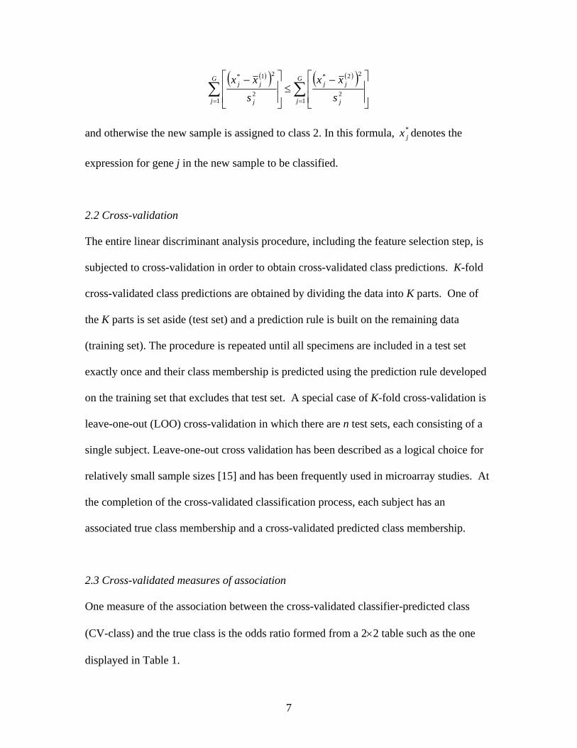
and otherwise the new sample is assigned to class 2. In this formula, denotes the

expression for gene j in the new sample to be classified.

*jx

2.2 Cross-validation

The entire linear discriminant analysis procedure, including the feature selection step, is

subjected to cross-validation in order to obtain cross-validated class predictions. K-fold

cross-validated class predictions are obtained by dividing the data into K parts. One of

the K parts is set aside (test set) and a prediction rule is built on the remaining data

(training set). The procedure is repeated until all specimens are included in a test set

exactly once and their class membership is predicted using the prediction rule developed

on the training set that excludes that test set. A special case of K-fold cross-validation is

leave-one-out (LOO) cross-validation in which there are n test sets, each consisting of a

single subject. Leave-one-out cross validation has been described as a logical choice for

relatively small sample sizes [15] and has been frequently used in microarray studies. At

the completion of the cross-validated classification process, each subject has an

associated true class membership and a cross-validated predicted class membership.

2.3 Cross-validated measures of association

One measure of the association between the cross-validated classifier-predicted class

(CV-class) and the true class is the odds ratio formed from a 2×2 table such as the one

displayed in Table 1.

7

(Insert Table 1 about here.)

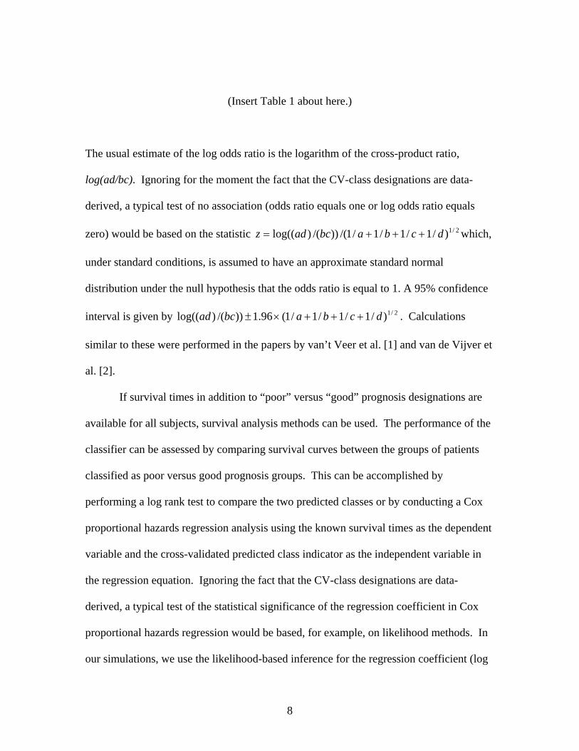
The usual estimate of the log odds ratio is the logarithm of the cross-product ratio,

log(ad/bc). Ignoring for the moment the fact that the CV-class designations are data-

derived, a typical test of no association (odds ratio equals one or log odds ratio equals

zero) would be based on the statistic which,

under standard conditions, is assumed to have an approximate standard normal

distribution under the null hypothesis that the odds ratio is equal to 1. A 95% confidence

interval is given by . Calculations

similar to these were performed in the papers by van’t Veer et al. [1] and van de Vijver et

al. [2].

2/1)/1/1/1/1/())/()log(( dcbabcadz +++=

2/1)/1/1/1/1(96.1))/()log(( dcbabcad +++×±

If survival times in addition to “poor” versus “good” prognosis designations are

available for all subjects, survival analysis methods can be used. The performance of the

classifier can be assessed by comparing survival curves between the groups of patients

classified as poor versus good prognosis groups. This can be accomplished by

performing a log rank test to compare the two predicted classes or by conducting a Cox

proportional hazards regression analysis using the known survival times as the dependent

variable and the cross-validated predicted class indicator as the independent variable in

the regression equation. Ignoring the fact that the CV-class designations are data-

derived, a typical test of the statistical significance of the regression coefficient in Cox

proportional hazards regression would be based, for example, on likelihood methods. In

our simulations, we use the likelihood-based inference for the regression coefficient (log

8

hazard ratio) as implemented by the coxph function of the survival library in the R

statistical package (http://www.r-project.org).

2.4 Data Simulation

To simulate data under the null case, gene expression profiles for each patient were

generated independently of the patients’ survival times. Expression measurements for

each of 10,000 genes were generated independently from the standard normal

distribution. All survival times were generated independently from an exponential

distribution with parameter lambda = −log(0.5)/10. This parameter was chosen to

produce an overall survival curve with probability of survival equal to 50% at 10 years.

Under the alternative case, survival times were generated to depend on gene

expression profiles. For each patient, 9900 genes were generated independently from a

standard normal distribution, while the remaining 100 genes were generated

independently from a normal distribution with mean µ1 and variance 1 for half of the

patients and from a normal distribution with mean µ2 and variance 1 for the other half.

The expression measures for these 100 genes were averaged for each patient to produce

scores s1, s2, . . ., sn. These scores were then used as the mean parameter (on the log-

scale) of the log normal distribution with variance 1, from which survival times were

simulated. Similarly to the null case, paired values of µ1 and µ2 were chosen so that on

average half of the subjects would have a survival time longer than 10 years.

The classifier building procedure was simulated as follows for both the null and

alternative cases. Patients were divided into poor and good prognosis groups on the basis

of their observed survival times. Subjects with observed survival time shorter than 10

9

years were assigned to poor prognosis class; others were assigned to the good prognosis

class. Survival times greater than 20 years were censored at 20 years. These assigned

outcome classes represented the “true” prognostic classes. On average, specimens were

equally distributed among the two classes due to the choice of parameters of the

distributions used to generate survival times. Univariate two-sample pooled variance t-

statistics comparing the good versus poor prognosis groups were computed for each gene,

and the 100 genes with largest absolute t-statistics were selected as the “informative

features” to be used in building the classifier. Fisher's diagonal linear discriminant

analysis was used to build the multivariate prediction rule using the 100 informative

genes to classify the specimens into the two prognosis groups. This entire classifier

building process was embedded in a cross-validation loop. For each training set,

informative genes were re-selected, the classifier was re-calculated, and the classifier was

used to make predictions on the test set. Note that the 100 gene sets selected as the

informative features in the training data sets were not guaranteed to be the genes that,

under the alternative case, were truly generated from two different distributions for the

good and poor prognosis groups. At the end of each simulated cross-validation, there

were true and cross-validated predicted prognosis classes assigned to each patient.

All simulations were repeated 10,000 times. For the null cases, situations with

25, 50, 100 and 500 subjects were considered, and leave-one-out, 10-fold and 5-fold

cross-validation were all examined. For simulations under alternative cases, the number

of subjects was always 100, and only leave-one-out cross-validation was considered.

While we would not usually advocate building classifiers using sample sizes as small as

25 or 50, we include them in our simulations because they cover the range of sample

10

sizes that have been used in published studies that developed microarray-based

classifiers. Also, we note that there were some iterations of the simulations for the small

sample size cases in which odds ratios or Cox regression coefficients could not be

calculated (e.g., empty cells in the 2×2 table), and we treated these as missing in the

simulation result summaries.

Under the null case, gene expression profiles are generated from the same

distribution for all patients, and class membership is defined independently from gene

expression profiles; therefore, there should be no significant association between true and

CV-class membership (log odds ratio = 0), and the regression coefficient of the CV-class

indicator variable in the Cox regression should not be statistically significantly different

from zero. For the null cases, our simulation studies examine for potential bias in the

estimates and problems with the level of tests of hypotheses of no association.

Under the alternative case, we expect there will be some association between the

CV-class and true class and survival. Therefore, we would expect a non-zero log odds

ratio and a non-zero regression coefficient for the cross-validated predicted class

indicator in the Cox regression. Due to the complexity of the classifier derivation, the

true values of the log odds ratio and regression coefficient are not easily calculated and

must be empirically determined by simulation. The true quantities were obtained

through an “inner” simulation loop, where at each “outer loop” of the primary simulation

we simulated 100 data sets of 100 subjects each from the same population from which the

original sample, on which the classifier was developed, was drawn. The classifier derived

on the full original data set was applied to each new (“inner loop”) data set. For each of

the 100 “inner loop” data sets, predicted (from full original sample classifier) class

11

memberships were obtained and log-odds ratios and Cox regression parameters were

estimated. These estimates were then averaged over the 100 inner loop data sets to

empirically determine the true log odds ratio and Cox regression coefficient. These true

quantities were compared to the cross-validated estimates obtained in the outer loop in

order to estimate bias and confidence interval coverage for the log odds ratio and Cox

regression coefficient. For confidence interval coverage, the coverage percentage was

broken into components, recording how often the true value falls completely below the

lower confidence bound (overestimation) and how often the true value falls completely

above the upper confidence bound (underestimation).

3. Results

3.1 Null case

Table 2 presents simulation results for the log odds ratio estimates calculated under a null

situation using various cross-validation methods. For leave-one-out cross-validation, the

mean estimated log odds ratio approached the correct value of zero as the sample size

increased but was strongly biased for small sample sizes. The estimated median log odds

ratio estimates suggested a trend of slightly more departure from the true value of zero

for 5-fold and 10-fold cross-validation compared to leave-one-out (LOO) cross-

validation, but there were no statistically significant differences in bias based on the mean

log odds ratio estimates. All of these cross-validation methods yielded log odds ratio

estimates with SDs substantially larger than the theoretical SD of (16/n)1/2 that would

apply to the situation in which all observations were independent and the predictions for

the n subjects were random “coin flips”. Additionally, we note that the use of 10-fold or

12

5-fold cross-validation resulted in considerably smaller estimated SD of the log odds ratio

estimate for sample size of 100. This may be related to the claim in the context of

prediction error estimation that LOO cross-validation often results in estimates with large

variance [11]. However, it is interesting to note that the degree of inflation of the SD

under LOO cross-validation (as a multiplier of the theoretical SD under independence)

may be less for smaller sample sizes.


Most dramatic and disturbing were the findings regarding the level of the tests of

significance of the log odds ratio. Table 3 shows that the observed rejection rates for the

z-test for no association greatly exceeded their nominal values. For example, if one were

to use leave-one-out cross-validation for a study of 100 subjects, a nominal 5% two-sided

z-test would reject the null hypothesis an estimated 41% of the time (23% lower

rejection, 18% upper rejection). The 18% upper rejection rate is probably of greatest

concern, as these might represent classifiers likely to be falsely reported as promising,

whereas classifiers exhibiting negative association with truth are unlikely to ever be

published. The problem with leave-one-out cross-validation is exacerbated with a larger

sample size. For a study of 500 subjects, the estimated rejection rate increased to nearly

55%. In part, this may be explained by greater inflation of the variance of the cross-

validated odds ratio estimate resulting from the proportion of overlapping observations (

(n-2)/(n-1) ) between any two leave-one-out training sets increasing with sample size (n).

Although the performance of the test is not quite as bad when 5-fold or 10-fold cross-

13

validation is used, the rejection rates for a study with sample size 100 still exceed the

nominal values by an unacceptably large margin. Similar results (not shown) were

observed for estimates and tests using the logistic regression-based estimate of log odds

ratio.


Table 4 presents simulation results for the log hazard ratio (Cox regression coefficient)

estimates calculated under the null situation using various cross-validation methods. The

results show trends analogous to those presented earlier for the log odds ratio. For leave-

one-out cross-validation, the mean estimated regression coefficient approached the

correct value of zero as the sample size increased. The estimated median regression

coefficient estimates suggested a trend of slightly more departure from the true value of

zero for 5-fold and 10-fold cross-validation compared to leave-one-out (LOO) cross-

validation, but there were no statistically significant differences in bias based on the mean

regression coefficient estimates. The use of 10-fold or 5-fold cross-validation resulted in

substantially smaller estimated SD of the regression coefficient estimate. All of these

cross-validation methods yielded coefficient estimates with SDs substantially larger than

the theoretical regression coefficient SD of (4/(expected number of events))1/2 that would

apply to the situation in which all observations were independent and the predictions for

the n subjects were random “coin flips”. (The expected number of events under the

simulation parameters considered is 0.75n.)

14


Similar to the case of testing the significance of the log odds ratio, our simulation

results presented in Table 5 show that the level of the likelihood ratio test for the Cox

regression coefficient was greatly inflated.


3.2 Alternative case

Table 6 presents results demonstrating properties of the odds ratio estimates, including

confidence interval coverage, under alternative cases in which there was a positive

association between gene expression profiles and survival outcomes. The degree of

separation of survival curves between the good and poor prognosis groups is controlled

by the two means used to generate the gene expression data which, in turn, influence the

means of the lognormal distributions generating the survival times. As the difference in

means decreases, the true log odds ratio between the true and predicted classes decreases

toward zero.


The results presented in table 6 show that for extremely large odds ratios, the confidence

interval coverage is not too far from the intended coverage probability. However, for

moderate or smaller odds ratios, confidence interval coverage can be quite poor. In any

15

case, it is noteworthy that the SDs of the estimated log odds ratios are very large relative

to the magnitude of the log odds ratios for a sample of size 100 which is typical of the

size of many gene expression microarray profiling studies. This implies that even if the

confidence intervals had correct coverage probabilities, the large variance of the

estimators may result in confidence intervals too wide to be helpful. In addition, it is

clear that the odds ratio can provide a misleading impression of the performance of the

predictor. For example, an odds ratio as large 17 (third case presented in Table 6) would

appear extremely impressive in the context of an epidemiologic study, but we see from

Table 6 that the corresponding classifier misclassification rate was a rather unsatisfying

20%.

4. Discussion

Cross-validation has been widely used to adjust for bias in estimates of prediction

accuracy of classifiers built from gene expression microarray profiling data when

independent data sets have not been available for testing the classifier. It performs well

for this purpose, although estimators may have large variance. Some authors of gene

expression microarray papers published in prominent biomedical medical journals have

attempted to take cross-validation one step further. Specifically, some authors have made

claims about the strength of a classifier by testing the statistical significance of

association between the true and cross-validated predicted prognostic classes. For

example, in Table 2 of the paper by van de Vijver et al. [2], some of the odds ratio

estimates presented are based on cross-validation, and confidence intervals and highly

significant p-values are reported. Our results in the present paper suggest that several of

16

these confidence intervals and p-values cannot be trusted. Particularly, we are concerned

that in the null case (classifier is completely uninformative), application of standard

inference procedures to test for significance of the association when cross-validation has

been used to determine predictions carries with it a very high likelihood of obtaining false

positive statistical significance. Our results also show that even if there is some modest

predictive value in the data-derived classifier, confidence intervals for the true association

between predicted and true prognostic class may be very wide and not have the reported

coverage properties. The problems arise from the fact that the data pairs (CV-class, True-

class) are not independent across subjects, and their dependency derives from re-use of

the true classes in the cross-validation process. This type of dependency violates the

assumptions of the standard statistical procedures for performing tests and constructing

confidence intervals for the measures of association. Finally, our results emphasized a

point made by others [16, 17] that measures of association such as an odds ratio are

generally poor gauges of classifier performance.

The next question is whether there are satisfactory remedies for these problems.

The most important point is to recognize that the prime interest is to evaluate the

classifier’s predictive accuracy and to determine if the accuracy is better than expected by

chance. Radmacher et al. [15] provide a valid method of testing whether the classifier

accuracy is better than expected by chance. They propose a permutation test on the

cross-validated misclassification rate. This test is performed directly on the cross-

validated prediction accuracy estimate and therefore avoids use of difficult to interpret

measures of association such as the odds ratio. The permutation approach involves

considering many possible permutations of assignments of clinical outcomes to profiles,

17

calculating for each permuted data set the cross-validated prediction accuracy. The

proportion of permutations for which the cross-validated accuracy calculated on the

original data set is better (larger) is a valid p-value for testing the null hypothesis that the

predictor performance is no better than chance.

If it is desired to assess predictor performance when adjusted for other covariates,

the permutation method of Radmacher et al. [15] cannot be directly applied. Tibshirani

and Efron [18] discuss the idea of “pre-validation” in logistic regression models in which

one of the variables in the model is a predicted class indicator obtained through cross-

validation and additional covariates can be incorporated into the regression model. They

point out a problem with the degrees of freedom in the test of the regression coefficient

for the predicted class indicator that is related to the problems with type I error rate and

confidence interval coverage we observed. We have elaborated on their findings to show

how seriously type I error rates and confidence interval non-coverage rates can be

inflated; we demonstrated the roles that sample size and method of cross-validation play,

and we presented results for Cox regression. The dependency problem we described in

the previous paragraph is essentially the phenomenon they describe as “information

leak”. They explore a bootstrap method to approximately correct the degrees of freedom

for testing regression coefficients. This seems like a promising approach, but would

require further investigation to determine how successfully the bootstrap-estimated

degrees of freedom can correct for problems in testing levels and confidence interval

coverage. Troendle et al. [19] demonstrated that bootstrap procedures may not perform

well in moderate to small samples of very high dimensional data. In addition, we would

be remiss if we did not point out that even if one were able to appropriately correct the

18

problems with the inference procedures, the variances of the measures of association

obtained through resampling of typical size gene expression microarray data sets would

still be very large. Also, it would be desirable to base the procedure on a more

interpretable alternative to the logistic regression coefficient such as gain in predictive

accuracy above predictive accuracy afforded by standard covariates.

In summary, our results provide further evidence that concerns recently expressed

[20, 21] about the reproducibility and validity of microarray-based prognostic classifiers

are warranted. Our findings support the notion that more and larger independent data sets

on which to develop and validate these classifiers are needed if microarray-based or other

molecular classifiers based on high-dimensional biologic data are ever to be important

clinical tools.

Acknowledgements

This study utilized the high-performance computational capabilities of the

Biowulf/LoBoS3 cluster at the National Institutes of Health, Bethesda, MD. We

gratefully acknowledge the funding provided by Ministero dell'Istruzione, dell'Università

e della Ricerca (grant PRIN 2003133820) and AIRC (Associazione Italiana per la Ricerca

sul Cancro, individual grant to M. A. Pierotti) to support Dr. Lusa’s participation in this

project.

19

References

1. van't Veer LJ, Dai HY, van de Vijver MJ, He YDD, Hart AAM, Mao M, Peterse HL,

van der Kooy K, Marton MJ, Witteveen AT, Schreiber GJ, Kerkhoven RM, Roberts C,

Linsley PS, Bernards R, Friend SH. Gene expression profiling predicts clinical outcome

of breast cancer. Nature 2002; 415(6871):530-536.

2. van de Vijver MJ, He YD, van’t Veer LJ, Dai H, Hart AAM, Voskuil DW, Schreiber

GJ, Peterse JL, Robert C, Marton MJ, Parrish M, Atsma D, Witteveen A, Glas A,

Delahaye L, van der Velde T, Bartelink H, Rodenhuis S, Rutgers ET, Friend SH,

Bernards R. A gene-expression signature as a predictor of survival in breast cancer. The

New England Journal of Medicine 2002; 347(25):1999-2009.

3. Beer DG, Kardia SLR, Huang CC, Giordano TJ, Levin AM, Misek DE, Lin L, Chen

G, Gharib TG, Thomas DG, Lizy ML, Kuick R, Hayasaka S, Taylor JMG, Iannettoni

MD, Orringer MB, Hanash S. Gene-expression profiles predict survival of patients with

lung adenocarcinoma. Nature Medicine 2002; 8(8):816-824.

4. Rosenwald A, Wright G, Chan WC, Connors JM, Campo E, Fisher RI, Gascoyne RD,

Muller-Hermelink HK, Smeland EB, Staudt LM for the Lymphoma/Leukemia Molecular

Profiling Project. The use of molecular profiling to predict survival after chemotherapy

for diffuse large B-cell lymphoma. The New England Journal of Medicine 2002;

346(25):1937-1947.

20

5. Shipp MA, Ross KN, Tamayo P, Weng AP, Kutok JL, Aguiar RCT, Gaasenbeek M,

Angelo M, Reich M, Pinkus GS, Ray TS, Koval MA, Last KW, Norton A, Lister TA,

Mesirov J, Neuberg DS, Lander ES, Aster JC, Golub TR. Diffuse large B-cell lymphoma

outcome prediction by gene-expression profiling and supervised machine learning.

Nature Medicine 2002; 8(1):68-74.

6. Tay ST, Leong SH, Yu K, Aggarwal A, Tan SY, Lee CH, Wong K, Visvanathan J,

Lim D, Wong WK, Soo KC, Kon OL, Tan P. A combined comparative genomic

hybridization and expression microarray analysis of gastric cancer reveals novel

molecular subtypes. Cancer Research 2003; 63(12):3309-3316.

7. Bullinger L, Dohner K, Bair E, Frohling S, Schlenk RF, Tibshirani R, Dohner H,

Pollack JR. Use of gene-expression profiling to identify prognostic subclasses in adult

acute myeloid leukemia. The New England Journal of Medicine 2004; 350(16):1605-

1616.

8. Valk PJM, Verhaak RGW, Beijen MA, Erpelinck CAJ, van Doorn-Khosrovani SBV,

Boer JM, Beverloo HB, Moorhouse MJ, van der Spek PJ, Lowenberg B, Delwel R.

Prognostically useful gene-expression profiles in acute myeloid leukemia. The New

England Journal of Medicine 2004; 350(16):1617-1628.

9. Dave SS, Wright G, Tan B, Rosenwald A, Gascoyne RD, Chan WC, Fisher RI, Braziel

RM, Rimsza LM, Grogan TM, Miller TP, LeBlanc M, Greiner TC, Weisenburger DD,

21

Lynch JC, Vose J, Armitage JO, Smeland EB, Kvaloy S, Holte H, Delabie J, Connors

JM, Lansdorp PM, Ouyang Q, Lister TA, Davies AJ, Norton AJ, Muller-Hermelink HK,

Ott G, Campo E, Montserrat E, Wilson WH, Jaffe ES, Simon R, Yang L, Powell J, Zhao

H, Goldschmidt N, Chiorazzi M, Staudt LM. Prediction of survival in follicular

lymphoma based on molecular features of tumor-infiltrating immune cells. The New

England Journal of Medicine 2004; 351(21):2159-2169.

10. Simon R, Radmacher MD, Dobbin K, McShane LM. Pitfalls in the use of DNA

microarray data for diagnostic and prognostic classification. Journal of the National

Cancer Institute 2003; 95(1):14-18.

11. Efron B. Estimating the error rate of a prediction rule: some improvements on cross-

validation. Journal of the American Statistical Association 1983; 78(382):316-331.

12. Efron B, Tibshirani R. Improvements on cross-validation: The .632+ bootstrap

method. Journal of the American Statistical Association 1997; 92(438):548-560.

13. Dudoit S, Fridlyand J, Speed TP. Comparison of discrimination methods for the

classification of tumors using gene expression data. Journal of the American Statistical

Association 2002; 97(457):77-87.

22

14. Simon R, Korn EL, McShane LM, Radmacher MD, Wright GW, Zhao Y. Design

and Analysis of DNA Microarray Investigations. Springer-Verlag: New York, 2004;

chapter 8.

15. Radmacher MD, McShane LM, Simon R. A paradigm for class prediction using gene

expression profiles. Journal of Computational Biology 2002; 9(3):505-511.

16. Pepe MS, Janes H, Longton G, Leisenring W, Newcomb P. Limitations of the odds

ratio in gauging performance of a diagnostic, prognostic, or screening marker. American

Journal of Epidemiology 2004; 159(9):882-890.

17. Kattan MW. Judging new markers by their ability to improve predictive accuracy.

Journal of the National Cancer Institute 2003; 95(9):634-635.

18. Tibshirani RJ, Efron B. Pre-validation and inference in microarrays. Statistical

Application in Genetics and Molecular Biology 2002; 1(1):1-18.

19. Troendle JF, Korn EL, McShane LM. An example of slow convergence of the

bootstrap in high dimensions. The American Statistician 2004; 58(1):25-29.

20. Michiels S, Koscielny S, Hill C. Prediction of cancer outcome with microarrays: a

multiple random validation strategy. Lancet 2005; 365(9458):488-492.

23

21. Ioannidis JPA. Microarrays and molecular research: noise discovery? Lancet 2005;

365(9458):454-455.

24

Table 1. 2×2 table for estimation of odds ratio. True-class Class 1 Class 2 Class 1 a b CV-class Class 2 c d

25

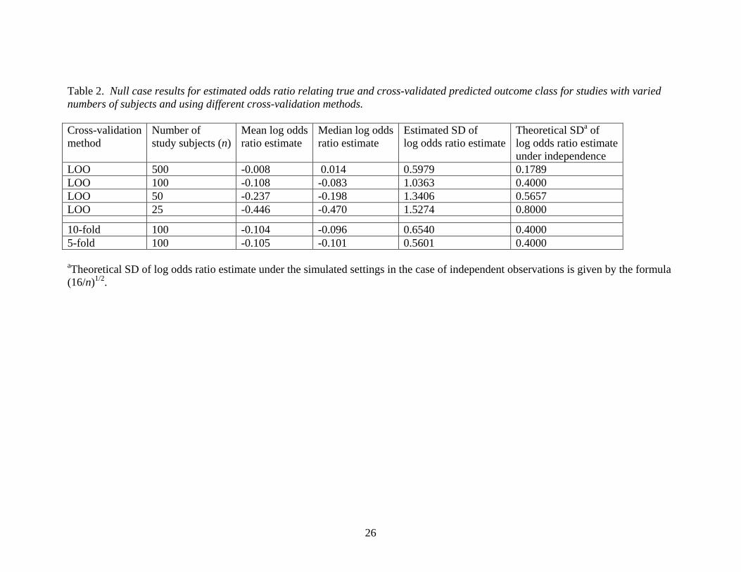
Table 2. Null case results for estimated odds ratio relating true and cross-validated predicted outcome class for studies with varied numbers of subjects and using different cross-validation methods. Cross-validation method

Number of study subjects (n)

Mean log oddsratio estimate

Median log oddsratio estimate

Estimated SD of log odds ratio estimate

Theoretical SDa of log odds ratio estimateunder independence

LOO 500 -0.008 0.014 0.5979 0.1789 LOO 100 -0.108 -0.083 1.0363 0.4000LOO 50 -0.237 -0.198 1.3406 0.5657LOO 25 -0.446 -0.470 1.5274 0.8000

10-fold 100 -0.104 -0.096 0.6540 0.40005-fold 100 -0.105 -0.101 0.5601 0.4000 aTheoretical SD of log odds ratio estimate under the simulated settings in the case of independent observations is given by the formula (16/n)1/2.

26

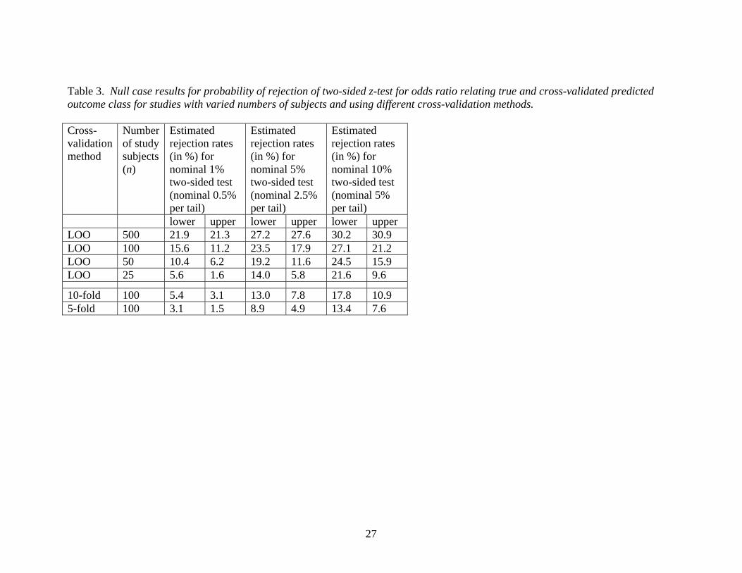
Table 3. Null case results for probability of rejection of two-sided z-test for odds ratio relating true and cross-validated predicted outcome class for studies with varied numbers of subjects and using different cross-validation methods. Cross-validation method


Estimated rejection rates (in %) for nominal 1% two-sided test (nominal 0.5% per tail)

Estimated rejection rates (in %) for nominal 5% two-sided test (nominal 2.5% per tail)

Estimated rejection rates (in %) for nominal 10% two-sided test (nominal 5% per tail)

lower upper lower upper lower upperLOO 500 21.9 21.3 27.2 27.6 30.2 30.9 LOO 100 15.6 11.2 23.5 17.9 27.1 21.2LOO 50 10.4 6.2 19.2 11.6 24.5 15.9LOO 25 5.6 1.6 14.0 5.8 21.6 9.6

10-fold 100 5.4 3.1 13.0 7.8 17.8 10.95-fold 100 3.1 1.5 8.9 4.9 13.4 7.6

27

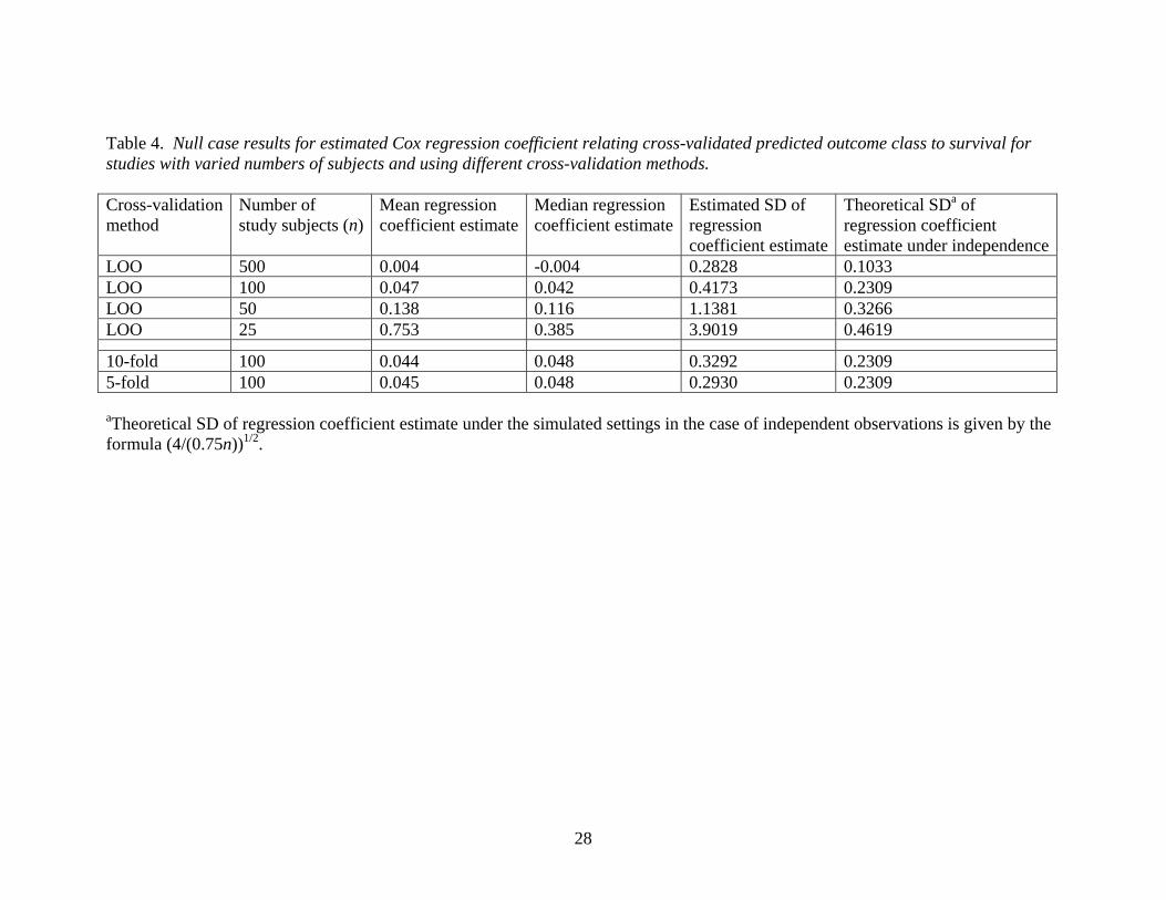
Table 4. Null case results for estimated Cox regression coefficient relating cross-validated predicted outcome class to survival for studies with varied numbers of subjects and using different cross-validation methods. Cross-validation method


Mean regression coefficient estimate

Median regression coefficient estimate

Estimated SD of regression coefficient estimate

Theoretical SDa of regression coefficient estimate under independence

LOO 500 0.004 -0.004 0.2828 0.1033 LOO 100 0.047 0.042 0.4173 0.2309LOO 50 0.138 0.116 1.1381 0.3266LOO 25 0.753 0.385 3.9019 0.4619

10-fold 100 0.044 0.048 0.3292 0.23095-fold 100 0.045 0.048 0.2930 0.2309 aTheoretical SD of regression coefficient estimate under the simulated settings in the case of independent observations is given by the formula (4/(0.75n))1/2.

28

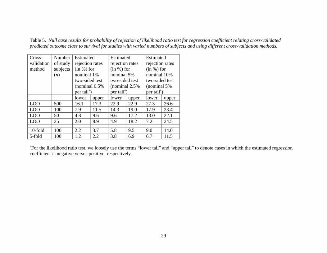
Table 5. Null case results for probability of rejection of likelihood ratio test for regression coefficient relating cross-validated predicted outcome class to survival for studies with varied numbers of subjects and using different cross-validation methods. Cross-validation method


Estimated rejection rates (in %) for nominal 1% two-sided test (nominal 0.5% per taila)

Estimated rejection rates (in %) for nominal 5% two-sided test (nominal 2.5% per taila)

Estimated rejection rates (in %) for nominal 10% two-sided test (nominal 5% per taila)

lower upper lower upper lower upperLOO 500 16.1 17.3 22.9 22.9 27.3 26.6 LOO 100 7.9 11.5 14.3 19.0 17.9 23.4LOO 50 4.8 9.6 9.6 17.2 13.0 22.1LOO 25 2.0 8.9 4.9 18.2 7.2 24.5

10-fold 100 2.2 3.7 5.8 9.5 9.0 14.05-fold 100 1.2 2.2 3.8 6.9 6.7 11.5 aFor the likelihood ratio test, we loosely use the terms “lower tail” and “upper tail” to denote cases in which the estimated regression coefficient is negative versus positive, respectively.

29

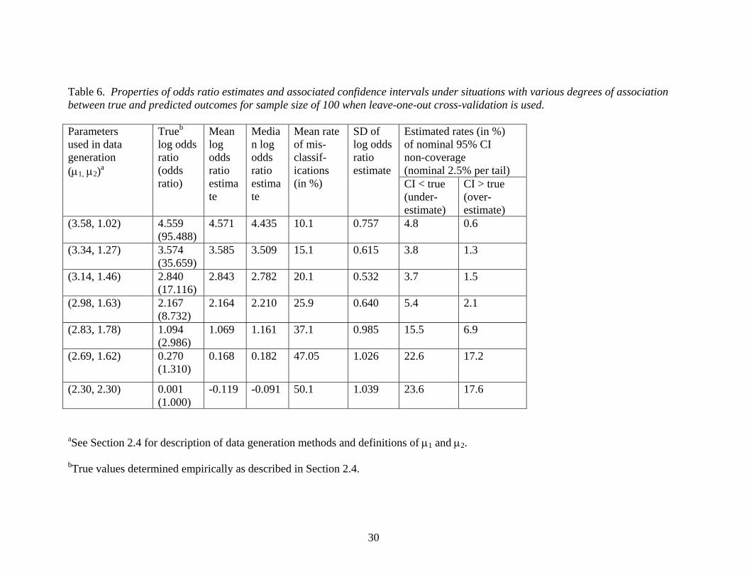
Table 6. Properties of odds ratio estimates and associated confidence intervals under situations with various degrees of association between true and predicted outcomes for sample size of 100 when leave-one-out cross-validation is used.

Estimated rates (in %) of nominal 95% CI non-coverage (nominal 2.5% per tail)

Parameters used in data generation (µ1, µ2)a

Trueb log odds ratio (odds ratio)

Mean log odds ratio estimate

Median log odds ratio estimate

Mean rate of mis-classif-ications (in %)

SD of log odds ratio estimate

CI < true (under-estimate)

CI > true (over- estimate)

(3.58, 1.02) 4.559 (95.488)

4.571 4.435 10.1 0.757 4.8 0.6

(3.34, 1.27) 3.574 (35.659)

3.585 3.509 15.1 0.615 3.8 1.3

(3.14, 1.46) 2.840 (17.116)

2.843 2.782 20.1 0.532 3.7 1.5

(2.98, 1.63) 2.167 (8.732)

2.164 2.210 25.9 0.640 5.4 2.1

(2.83, 1.78) 1.094 (2.986)

1.069 1.161 37.1 0.985 15.5 6.9

(2.69, 1.62) 0.270 (1.310)

0.168 0.182 47.05 1.026 22.6 17.2

(2.30, 2.30) 0.001 (1.000)

-0.119 -0.091 50.1 1.039 23.6 17.6

aSee Section 2.4 for description of data generation methods and definitions of µ1 and µ2. bTrue values determined empirically as described in Section 2.4.

30

appropriateness of some resampling-based inference

Documents