13: resampling filters halfband filters polynomial ... · pdf file13: resampling filters 13:...
TRANSCRIPT
13: Resampling Filters
13: Resampling Filters
• Resampling
• Halfband Filters
• Dyadic 1:8 Upsampler
• Rational Resampling
• Arbitrary Resampling +
• Polynomial Approximation
• Farrow Filter +
• Summary
• MATLAB routines
DSP and Digital Filters (2017-10126) Resampling: 13 – 1 / 10
Resampling
13: Resampling Filters
• Resampling
• Halfband Filters
• Dyadic 1:8 Upsampler
• Rational Resampling
• Arbitrary Resampling +
• Polynomial Approximation
• Farrow Filter +
• Summary
• MATLAB routines
DSP and Digital Filters (2017-10126) Resampling: 13 – 2 / 10
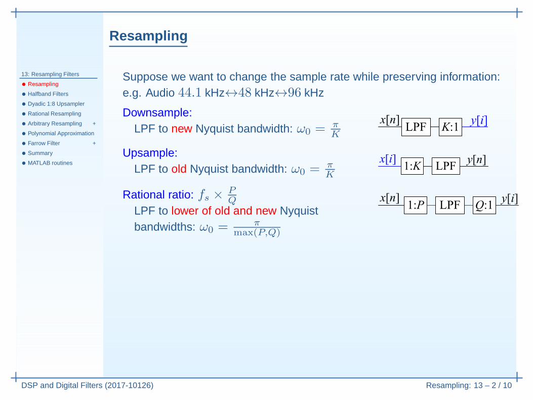
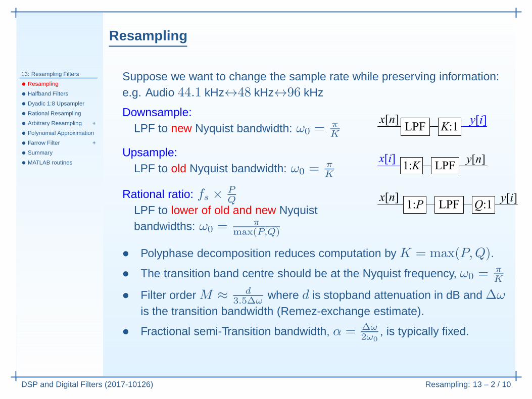
Suppose we want to change the sample rate while preserving information:e.g. Audio 44.1 kHz↔48 kHz↔96 kHz
Resampling
13: Resampling Filters
• Resampling
• Halfband Filters
• Dyadic 1:8 Upsampler
• Rational Resampling
• Arbitrary Resampling +
• Polynomial Approximation
• Farrow Filter +
• Summary
• MATLAB routines
DSP and Digital Filters (2017-10126) Resampling: 13 – 2 / 10
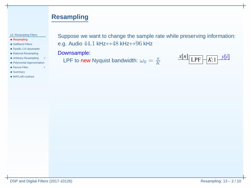
Suppose we want to change the sample rate while preserving information:e.g. Audio 44.1 kHz↔48 kHz↔96 kHz
Downsample:LPF to new Nyquist bandwidth: ω0 = π
K
Resampling
13: Resampling Filters
• Resampling
• Halfband Filters
• Dyadic 1:8 Upsampler
• Rational Resampling
• Arbitrary Resampling +
• Polynomial Approximation
• Farrow Filter +
• Summary
• MATLAB routines
DSP and Digital Filters (2017-10126) Resampling: 13 – 2 / 10
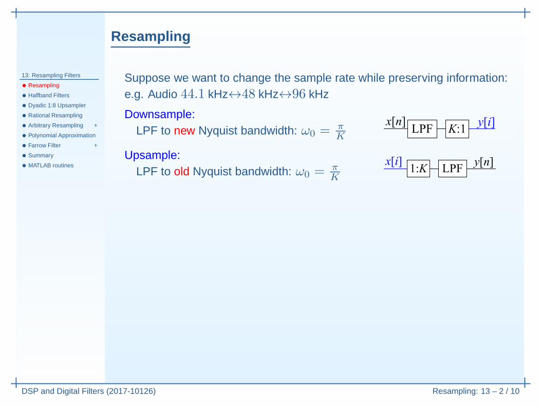
Suppose we want to change the sample rate while preserving information:e.g. Audio 44.1 kHz↔48 kHz↔96 kHz
Downsample:LPF to new Nyquist bandwidth: ω0 = π
K
Upsample:LPF to old Nyquist bandwidth: ω0 = π
K
Resampling
13: Resampling Filters
• Resampling
• Halfband Filters
• Dyadic 1:8 Upsampler
• Rational Resampling
• Arbitrary Resampling +
• Polynomial Approximation
• Farrow Filter +
• Summary
• MATLAB routines
DSP and Digital Filters (2017-10126) Resampling: 13 – 2 / 10
Suppose we want to change the sample rate while preserving information:e.g. Audio 44.1 kHz↔48 kHz↔96 kHz
Downsample:LPF to new Nyquist bandwidth: ω0 = π
K
Upsample:LPF to old Nyquist bandwidth: ω0 = π
K
Rational ratio: fs ×PQ
LPF to lower of old and new Nyquistbandwidths: ω0 = π
max(P,Q)
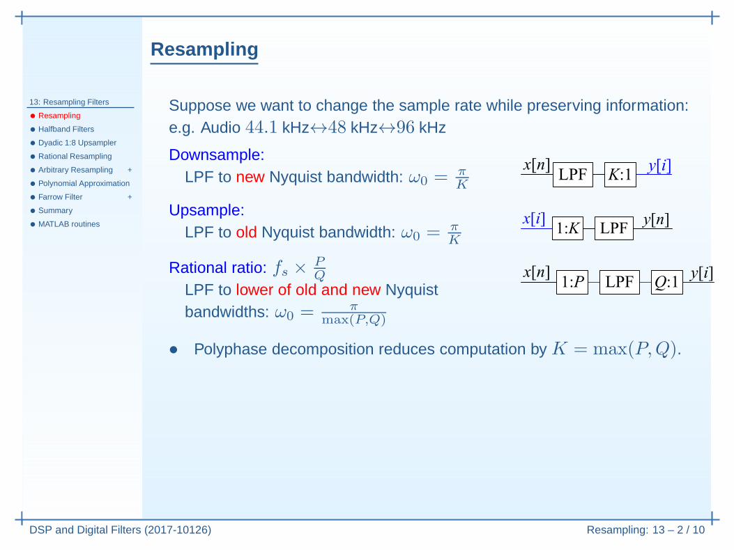
• Polyphase decomposition reduces computation by K = max(P,Q).
Resampling
13: Resampling Filters
• Resampling
• Halfband Filters
• Dyadic 1:8 Upsampler
• Rational Resampling
• Arbitrary Resampling +
• Polynomial Approximation
• Farrow Filter +
• Summary
• MATLAB routines
DSP and Digital Filters (2017-10126) Resampling: 13 – 2 / 10
Suppose we want to change the sample rate while preserving information:e.g. Audio 44.1 kHz↔48 kHz↔96 kHz
Downsample:LPF to new Nyquist bandwidth: ω0 = π
K
Upsample:LPF to old Nyquist bandwidth: ω0 = π
K
Rational ratio: fs ×PQ
LPF to lower of old and new Nyquistbandwidths: ω0 = π
max(P,Q)
• Polyphase decomposition reduces computation by K = max(P,Q).
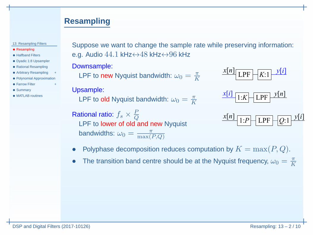
• The transition band centre should be at the Nyquist frequency, ω0 = πK
Resampling
13: Resampling Filters
• Resampling
• Halfband Filters
• Dyadic 1:8 Upsampler
• Rational Resampling
• Arbitrary Resampling +
• Polynomial Approximation
• Farrow Filter +
• Summary
• MATLAB routines
DSP and Digital Filters (2017-10126) Resampling: 13 – 2 / 10
Suppose we want to change the sample rate while preserving information:e.g. Audio 44.1 kHz↔48 kHz↔96 kHz
Downsample:LPF to new Nyquist bandwidth: ω0 = π
K
Upsample:LPF to old Nyquist bandwidth: ω0 = π
K
Rational ratio: fs ×PQ
LPF to lower of old and new Nyquistbandwidths: ω0 = π
max(P,Q)
• Polyphase decomposition reduces computation by K = max(P,Q).
• The transition band centre should be at the Nyquist frequency, ω0 = πK
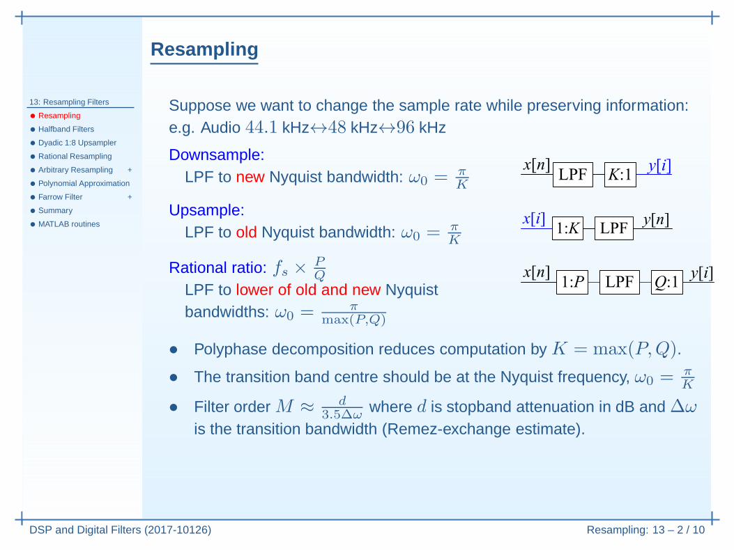
• Filter order M ≈ d3.5∆ω
where d is stopband attenuation in dB and ∆ω
is the transition bandwidth (Remez-exchange estimate).
Resampling
13: Resampling Filters
• Resampling
• Halfband Filters
• Dyadic 1:8 Upsampler
• Rational Resampling
• Arbitrary Resampling +
• Polynomial Approximation
• Farrow Filter +
• Summary
• MATLAB routines
DSP and Digital Filters (2017-10126) Resampling: 13 – 2 / 10
Suppose we want to change the sample rate while preserving information:e.g. Audio 44.1 kHz↔48 kHz↔96 kHz
Downsample:LPF to new Nyquist bandwidth: ω0 = π
K
Upsample:LPF to old Nyquist bandwidth: ω0 = π
K
Rational ratio: fs ×PQ
LPF to lower of old and new Nyquistbandwidths: ω0 = π
max(P,Q)
• Polyphase decomposition reduces computation by K = max(P,Q).
• The transition band centre should be at the Nyquist frequency, ω0 = πK
• Filter order M ≈ d3.5∆ω
where d is stopband attenuation in dB and ∆ω
is the transition bandwidth (Remez-exchange estimate).
• Fractional semi-Transition bandwidth, α = ∆ω2ω0
, is typically fixed.
e.g. α = 0.05 ⇒ M ≈ dK7πα = 0.9dK (where ω0 = π
K)
Halfband Filters
13: Resampling Filters
• Resampling
• Halfband Filters
• Dyadic 1:8 Upsampler
• Rational Resampling
• Arbitrary Resampling +
• Polynomial Approximation
• Farrow Filter +
• Summary
• MATLAB routines
DSP and Digital Filters (2017-10126) Resampling: 13 – 3 / 10
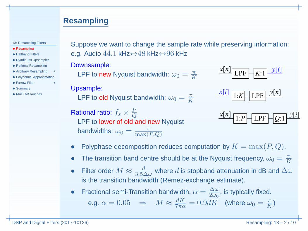
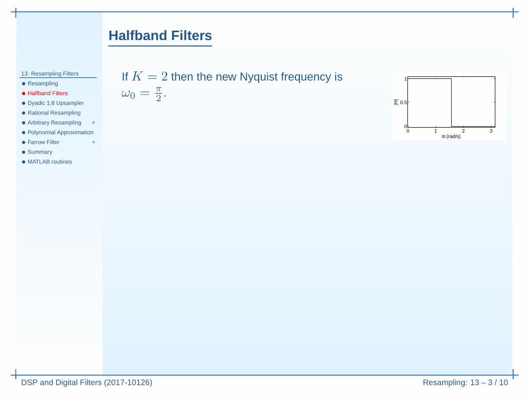
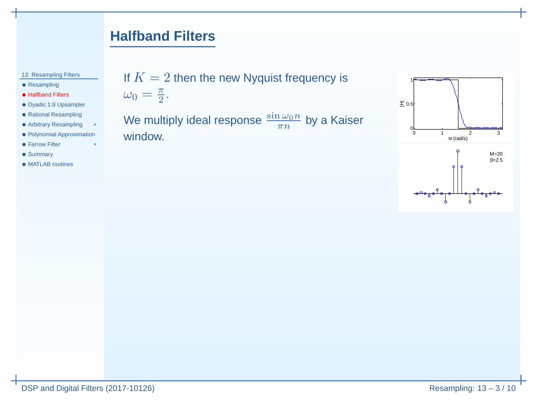
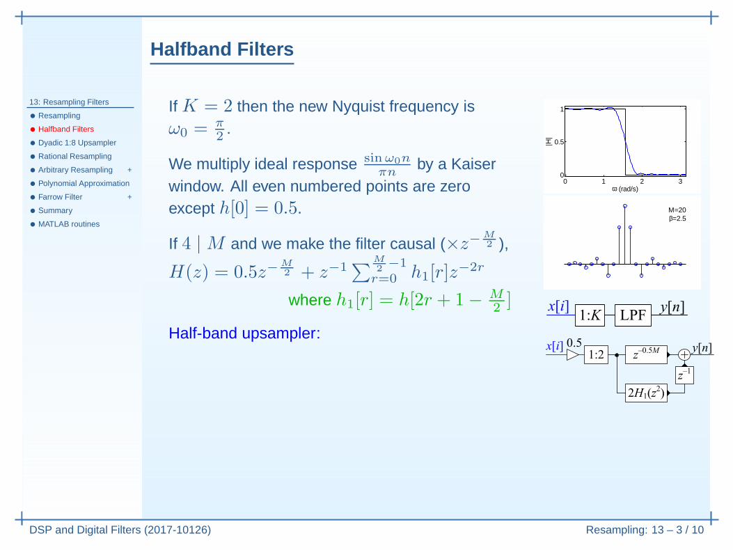
If K = 2 then the new Nyquist frequency isω0 = π
2 .
0 1 2 30
0.5
1
ω (rad/s)
Halfband Filters
13: Resampling Filters
• Resampling
• Halfband Filters
• Dyadic 1:8 Upsampler
• Rational Resampling
• Arbitrary Resampling +
• Polynomial Approximation
• Farrow Filter +
• Summary
• MATLAB routines
DSP and Digital Filters (2017-10126) Resampling: 13 – 3 / 10
If K = 2 then the new Nyquist frequency isω0 = π
2 .
We multiply ideal response sinω0nπn
by a Kaiserwindow. 0 1 2 3
0
0.5
1
ω (rad/s)
M=20β=2.5
Halfband Filters
13: Resampling Filters
• Resampling
• Halfband Filters
• Dyadic 1:8 Upsampler
• Rational Resampling
• Arbitrary Resampling +
• Polynomial Approximation
• Farrow Filter +
• Summary
• MATLAB routines
DSP and Digital Filters (2017-10126) Resampling: 13 – 3 / 10
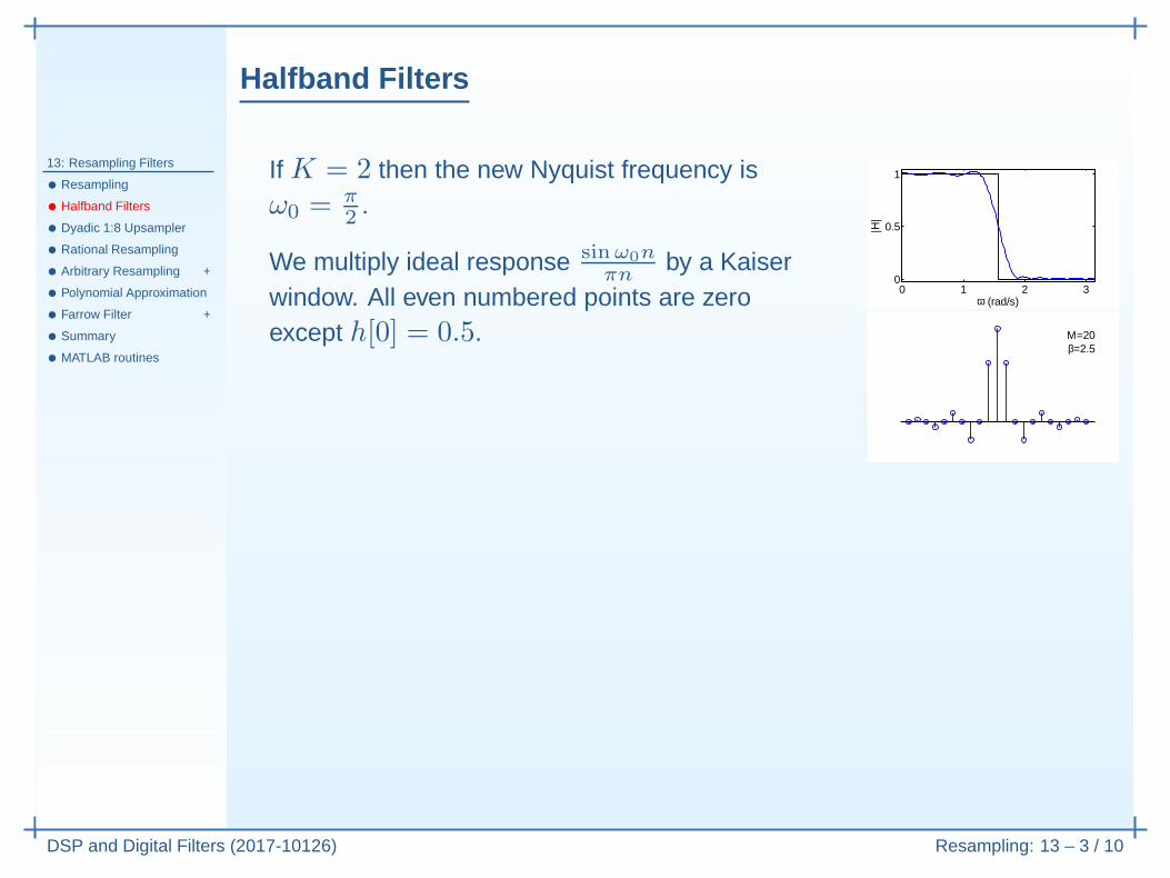
If K = 2 then the new Nyquist frequency isω0 = π
2 .
We multiply ideal response sinω0nπn
by a Kaiserwindow. All even numbered points are zeroexcept h[0] = 0.5.
0 1 2 30
0.5
1
ω (rad/s)
M=20β=2.5
Halfband Filters
13: Resampling Filters
• Resampling
• Halfband Filters
• Dyadic 1:8 Upsampler
• Rational Resampling
• Arbitrary Resampling +
• Polynomial Approximation
• Farrow Filter +
• Summary
• MATLAB routines
DSP and Digital Filters (2017-10126) Resampling: 13 – 3 / 10
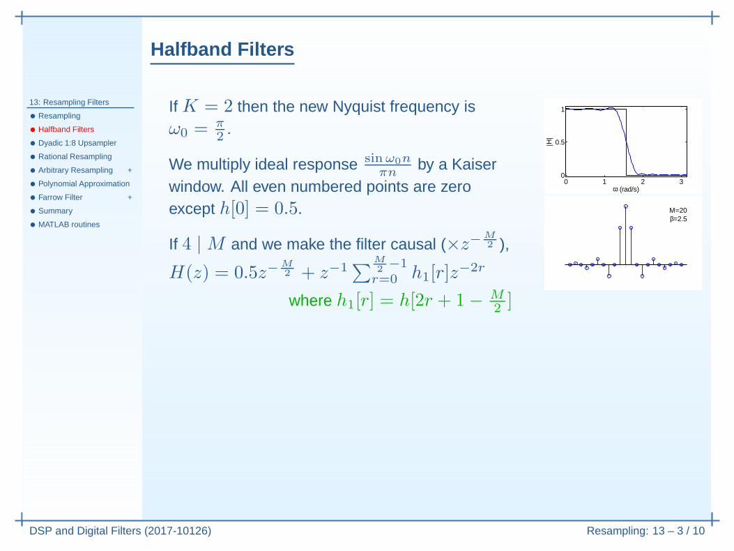
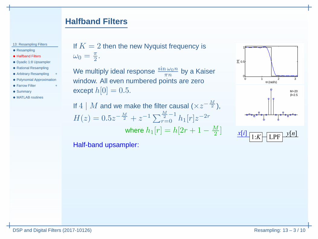
If K = 2 then the new Nyquist frequency isω0 = π
2 .
We multiply ideal response sinω0nπn
by a Kaiserwindow. All even numbered points are zeroexcept h[0] = 0.5.
If 4 | M and we make the filter causal (×z−M2 ),
H(z) = 0.5z−M2 + z−1
∑
M2−1
r=0 h1[r]z−2r
where h1[r] = h[2r + 1− M2 ]
0 1 2 30
0.5
1
ω (rad/s)
M=20β=2.5
Halfband Filters
13: Resampling Filters
• Resampling
• Halfband Filters
• Dyadic 1:8 Upsampler
• Rational Resampling
• Arbitrary Resampling +
• Polynomial Approximation
• Farrow Filter +
• Summary
• MATLAB routines
DSP and Digital Filters (2017-10126) Resampling: 13 – 3 / 10
If K = 2 then the new Nyquist frequency isω0 = π
2 .
We multiply ideal response sinω0nπn
by a Kaiserwindow. All even numbered points are zeroexcept h[0] = 0.5.
If 4 | M and we make the filter causal (×z−M2 ),
H(z) = 0.5z−M2 + z−1
∑
M2−1
r=0 h1[r]z−2r
where h1[r] = h[2r + 1− M2 ]
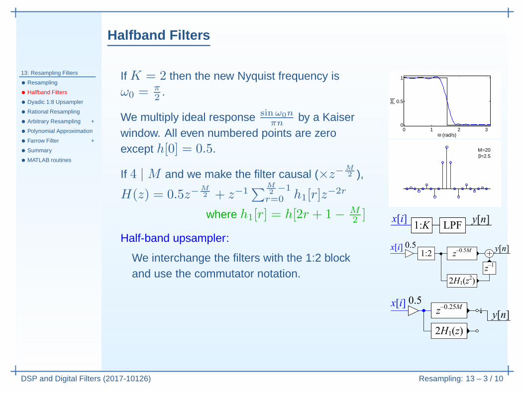
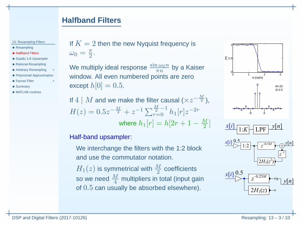
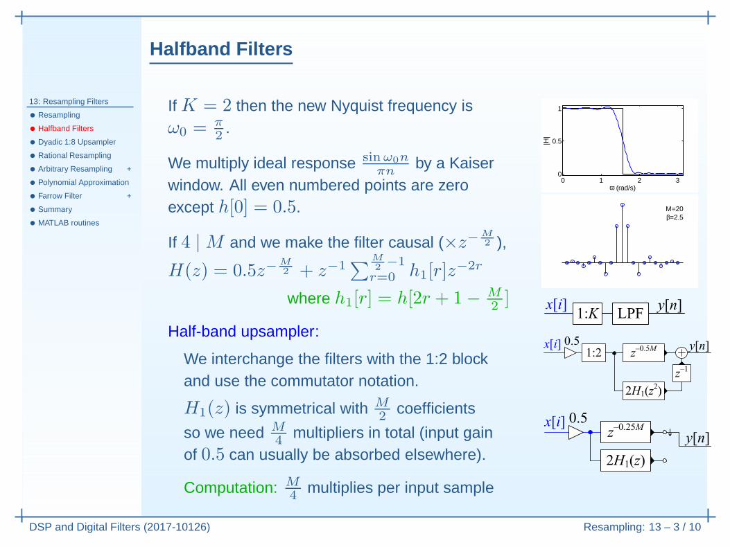
Half-band upsampler:
0 1 2 30
0.5
1
ω (rad/s)
M=20β=2.5
Halfband Filters
13: Resampling Filters
• Resampling
• Halfband Filters
• Dyadic 1:8 Upsampler
• Rational Resampling
• Arbitrary Resampling +
• Polynomial Approximation
• Farrow Filter +
• Summary
• MATLAB routines
DSP and Digital Filters (2017-10126) Resampling: 13 – 3 / 10
If K = 2 then the new Nyquist frequency isω0 = π
2 .
We multiply ideal response sinω0nπn
by a Kaiserwindow. All even numbered points are zeroexcept h[0] = 0.5.
If 4 | M and we make the filter causal (×z−M2 ),
H(z) = 0.5z−M2 + z−1
∑
M2−1
r=0 h1[r]z−2r
where h1[r] = h[2r + 1− M2 ]
Half-band upsampler:
We interchange the filters with the 1:2 blockand use the commutator notation.
H1(z) is symmetrical with M2 coefficients
so we need M4 multipliers in total (input gain
of 0.5 can usually be absorbed elsewhere).
Computation: M4 multiplies per input sample
0 1 2 30
0.5
1
ω (rad/s)
M=20β=2.5
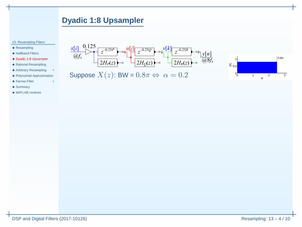
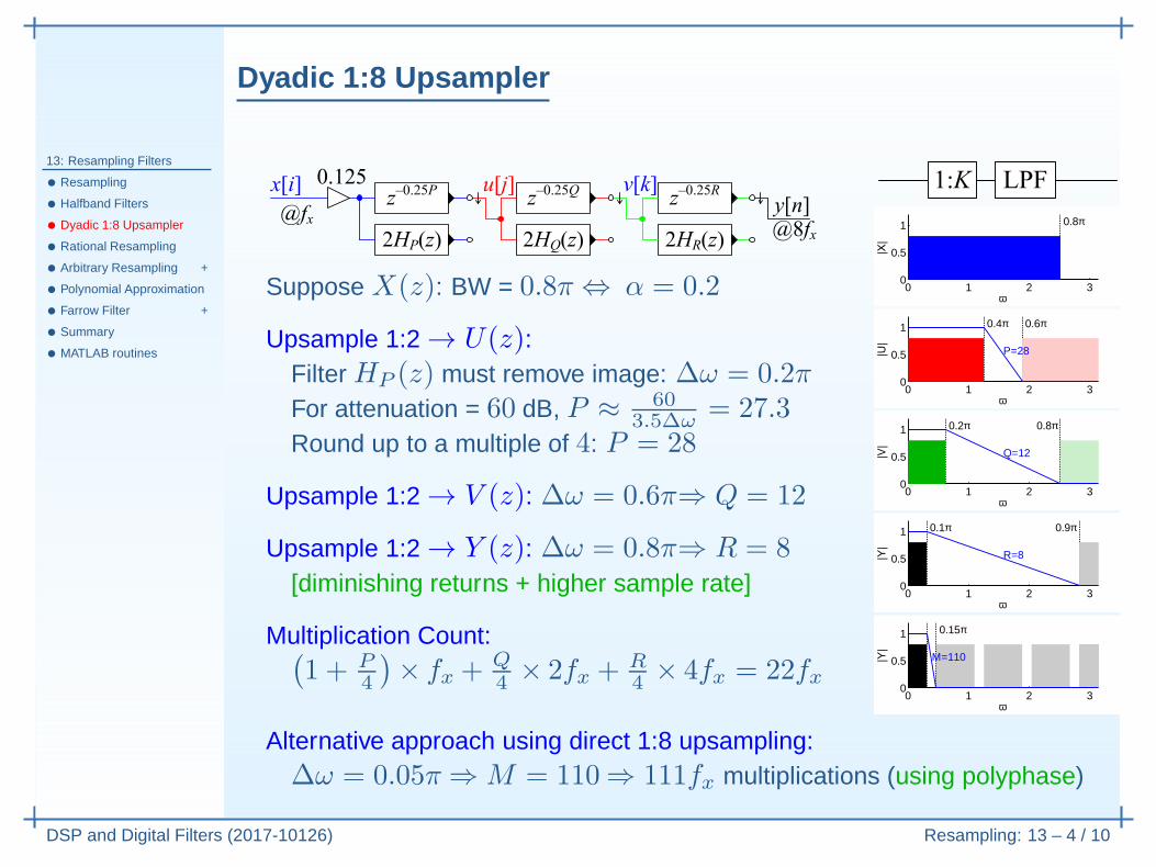
Dyadic 1:8 Upsampler
13: Resampling Filters
• Resampling
• Halfband Filters
• Dyadic 1:8 Upsampler
• Rational Resampling
• Arbitrary Resampling +
• Polynomial Approximation
• Farrow Filter +
• Summary
• MATLAB routines
DSP and Digital Filters (2017-10126) Resampling: 13 – 4 / 10
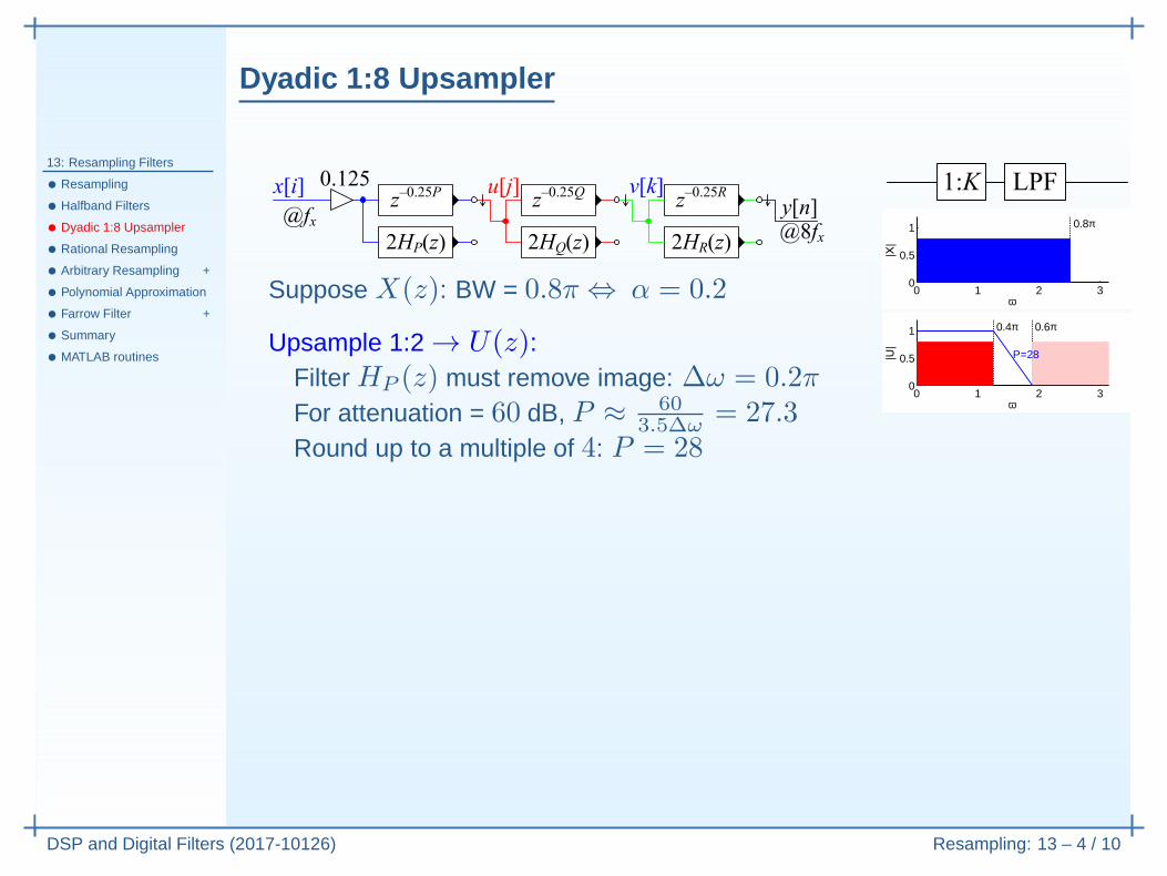
Suppose X(z): BW = 0.8π ⇔ α = 0.2 0 1 2 30
0.5
1 0.8π
ω
Dyadic 1:8 Upsampler
13: Resampling Filters
• Resampling
• Halfband Filters
• Dyadic 1:8 Upsampler
• Rational Resampling
• Arbitrary Resampling +
• Polynomial Approximation
• Farrow Filter +
• Summary
• MATLAB routines
DSP and Digital Filters (2017-10126) Resampling: 13 – 4 / 10
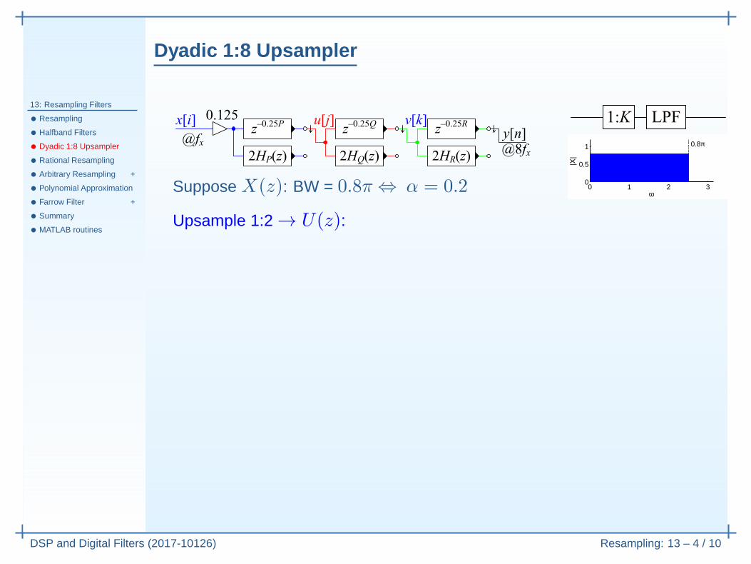
Suppose X(z): BW = 0.8π ⇔ α = 0.2
Upsample 1:2 → U(z):
0 1 2 30
0.5
1 0.8π
ω
Dyadic 1:8 Upsampler
13: Resampling Filters
• Resampling
• Halfband Filters
• Dyadic 1:8 Upsampler
• Rational Resampling
• Arbitrary Resampling +
• Polynomial Approximation
• Farrow Filter +
• Summary
• MATLAB routines
DSP and Digital Filters (2017-10126) Resampling: 13 – 4 / 10
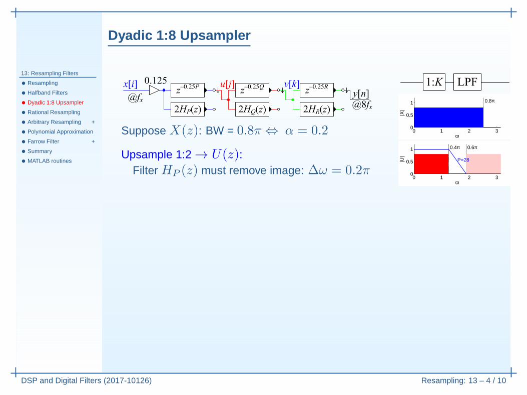
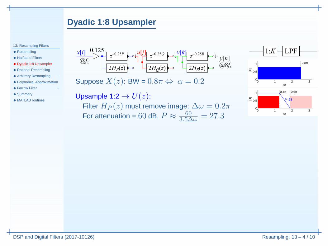
Suppose X(z): BW = 0.8π ⇔ α = 0.2
Upsample 1:2 → U(z):Filter HP (z) must remove image: ∆ω = 0.2π
0 1 2 30
0.5
1 0.8π
ω
0 1 2 30
0.5
1 0.4π 0.6π
P=28
ω
Dyadic 1:8 Upsampler
13: Resampling Filters
• Resampling
• Halfband Filters
• Dyadic 1:8 Upsampler
• Rational Resampling
• Arbitrary Resampling +
• Polynomial Approximation
• Farrow Filter +
• Summary
• MATLAB routines
DSP and Digital Filters (2017-10126) Resampling: 13 – 4 / 10
Suppose X(z): BW = 0.8π ⇔ α = 0.2
Upsample 1:2 → U(z):Filter HP (z) must remove image: ∆ω = 0.2πFor attenuation = 60 dB, P ≈ 60
3.5∆ω= 27.3
0 1 2 30
0.5
1 0.8π
ω
0 1 2 30
0.5
1 0.4π 0.6π
P=28
ω
Dyadic 1:8 Upsampler
13: Resampling Filters
• Resampling
• Halfband Filters
• Dyadic 1:8 Upsampler
• Rational Resampling
• Arbitrary Resampling +
• Polynomial Approximation
• Farrow Filter +
• Summary
• MATLAB routines
DSP and Digital Filters (2017-10126) Resampling: 13 – 4 / 10
Suppose X(z): BW = 0.8π ⇔ α = 0.2
Upsample 1:2 → U(z):Filter HP (z) must remove image: ∆ω = 0.2πFor attenuation = 60 dB, P ≈ 60
3.5∆ω= 27.3
Round up to a multiple of 4: P = 28
0 1 2 30
0.5
1 0.8π
ω
0 1 2 30
0.5
1 0.4π 0.6π
P=28
ω
Dyadic 1:8 Upsampler
13: Resampling Filters
• Resampling
• Halfband Filters
• Dyadic 1:8 Upsampler
• Rational Resampling
• Arbitrary Resampling +
• Polynomial Approximation
• Farrow Filter +
• Summary
• MATLAB routines
DSP and Digital Filters (2017-10126) Resampling: 13 – 4 / 10
Suppose X(z): BW = 0.8π ⇔ α = 0.2
Upsample 1:2 → U(z):Filter HP (z) must remove image: ∆ω = 0.2πFor attenuation = 60 dB, P ≈ 60
3.5∆ω= 27.3
Round up to a multiple of 4: P = 28
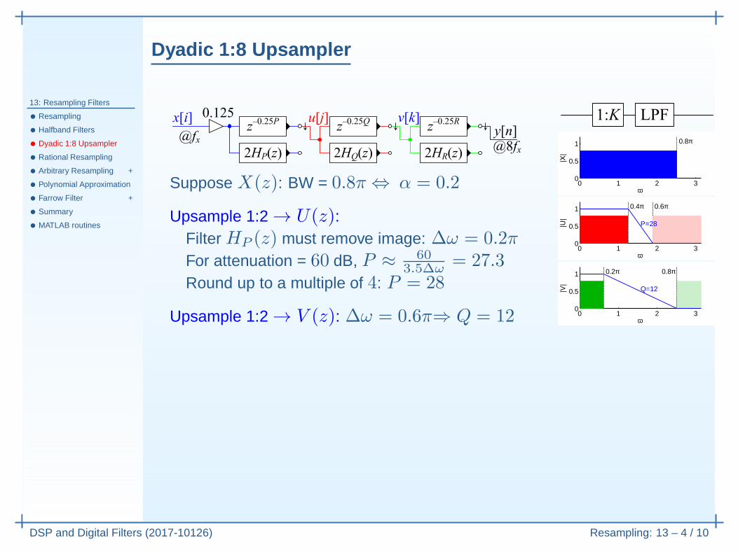
Upsample 1:2 → V (z): ∆ω = 0.6π⇒ Q = 12
0 1 2 30
0.5
1 0.8π
ω
0 1 2 30
0.5
1 0.4π 0.6π
P=28
ω
0 1 2 30
0.5
1 0.2π 0.8π
Q=12
ω
Dyadic 1:8 Upsampler
13: Resampling Filters
• Resampling
• Halfband Filters
• Dyadic 1:8 Upsampler
• Rational Resampling
• Arbitrary Resampling +
• Polynomial Approximation
• Farrow Filter +
• Summary
• MATLAB routines
DSP and Digital Filters (2017-10126) Resampling: 13 – 4 / 10
Suppose X(z): BW = 0.8π ⇔ α = 0.2
Upsample 1:2 → U(z):Filter HP (z) must remove image: ∆ω = 0.2πFor attenuation = 60 dB, P ≈ 60
3.5∆ω= 27.3
Round up to a multiple of 4: P = 28
Upsample 1:2 → V (z): ∆ω = 0.6π⇒ Q = 12
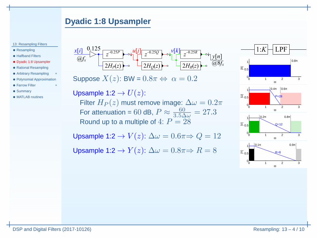
Upsample 1:2 → Y (z): ∆ω = 0.8π⇒ R = 8
0 1 2 30
0.5
1 0.8π
ω
0 1 2 30
0.5
1 0.4π 0.6π
P=28
ω
0 1 2 30
0.5
1 0.2π 0.8π
Q=12
ω
0 1 2 30
0.5
1 0.1π 0.9π
R=8
ω
Dyadic 1:8 Upsampler
13: Resampling Filters
• Resampling
• Halfband Filters
• Dyadic 1:8 Upsampler
• Rational Resampling
• Arbitrary Resampling +
• Polynomial Approximation
• Farrow Filter +
• Summary
• MATLAB routines
DSP and Digital Filters (2017-10126) Resampling: 13 – 4 / 10
Suppose X(z): BW = 0.8π ⇔ α = 0.2
Upsample 1:2 → U(z):Filter HP (z) must remove image: ∆ω = 0.2πFor attenuation = 60 dB, P ≈ 60
3.5∆ω= 27.3
Round up to a multiple of 4: P = 28
Upsample 1:2 → V (z): ∆ω = 0.6π⇒ Q = 12
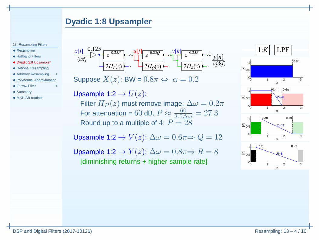
Upsample 1:2 → Y (z): ∆ω = 0.8π⇒ R = 8[diminishing returns + higher sample rate]
0 1 2 30
0.5
1 0.8π
ω
0 1 2 30
0.5
1 0.4π 0.6π
P=28
ω
0 1 2 30
0.5
1 0.2π 0.8π
Q=12
ω
0 1 2 30
0.5
1 0.1π 0.9π
R=8
ω
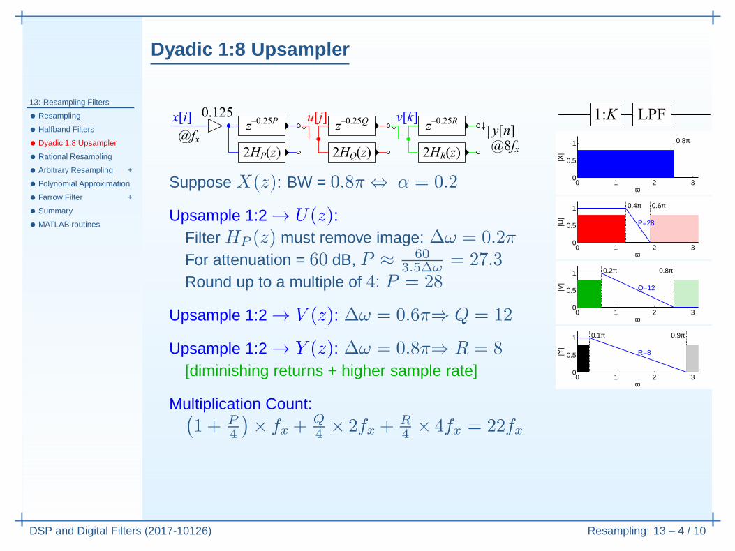
Dyadic 1:8 Upsampler
13: Resampling Filters
• Resampling
• Halfband Filters
• Dyadic 1:8 Upsampler
• Rational Resampling
• Arbitrary Resampling +
• Polynomial Approximation
• Farrow Filter +
• Summary
• MATLAB routines
DSP and Digital Filters (2017-10126) Resampling: 13 – 4 / 10
Suppose X(z): BW = 0.8π ⇔ α = 0.2
Upsample 1:2 → U(z):Filter HP (z) must remove image: ∆ω = 0.2πFor attenuation = 60 dB, P ≈ 60
3.5∆ω= 27.3
Round up to a multiple of 4: P = 28
Upsample 1:2 → V (z): ∆ω = 0.6π⇒ Q = 12
Upsample 1:2 → Y (z): ∆ω = 0.8π⇒ R = 8[diminishing returns + higher sample rate]
Multiplication Count:(
1 + P4
)
× fx +Q
4 × 2fx +R4 × 4fx = 22fx
0 1 2 30
0.5
1 0.8π
ω
0 1 2 30
0.5
1 0.4π 0.6π
P=28
ω
0 1 2 30
0.5
1 0.2π 0.8π
Q=12
ω
0 1 2 30
0.5
1 0.1π 0.9π
R=8
ω
0 1 2 30
0.5
1 0.15π
M=110
ω
Alternative approach using direct 1:8 upsampling:∆ω = 0.05π ⇒ M = 110⇒ 111fx multiplications (using polyphase)
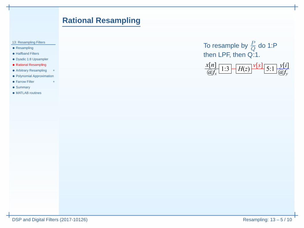
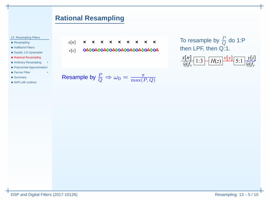
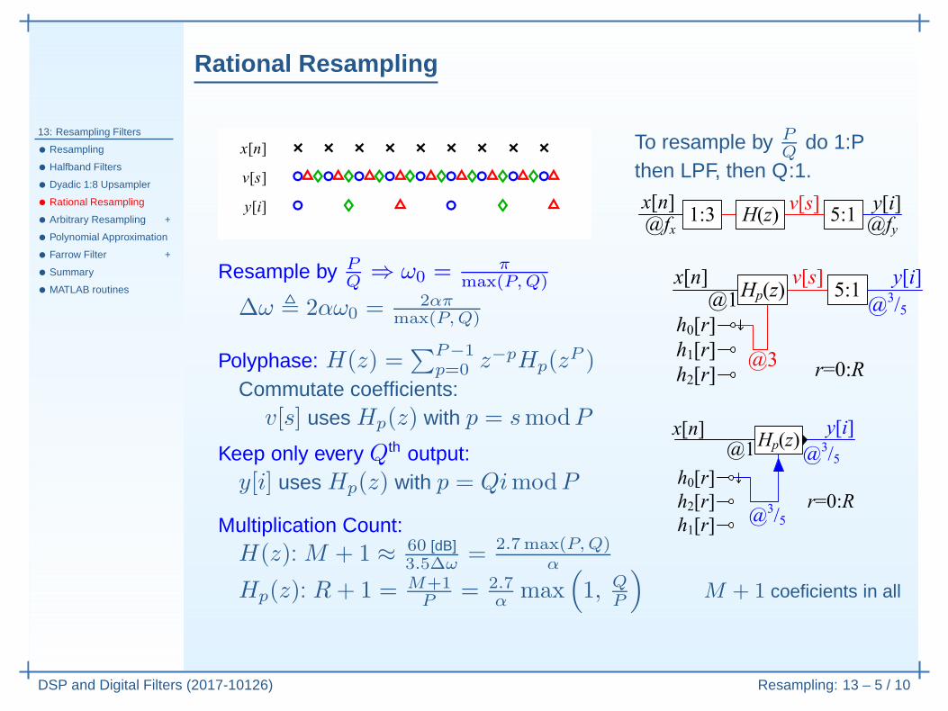
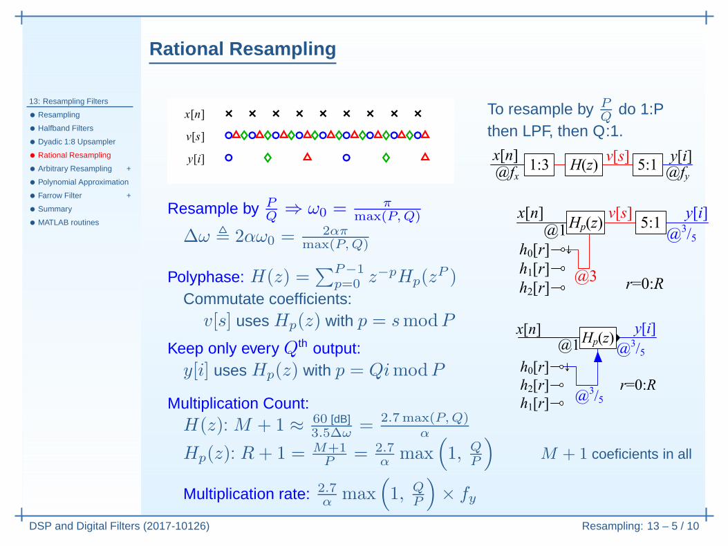
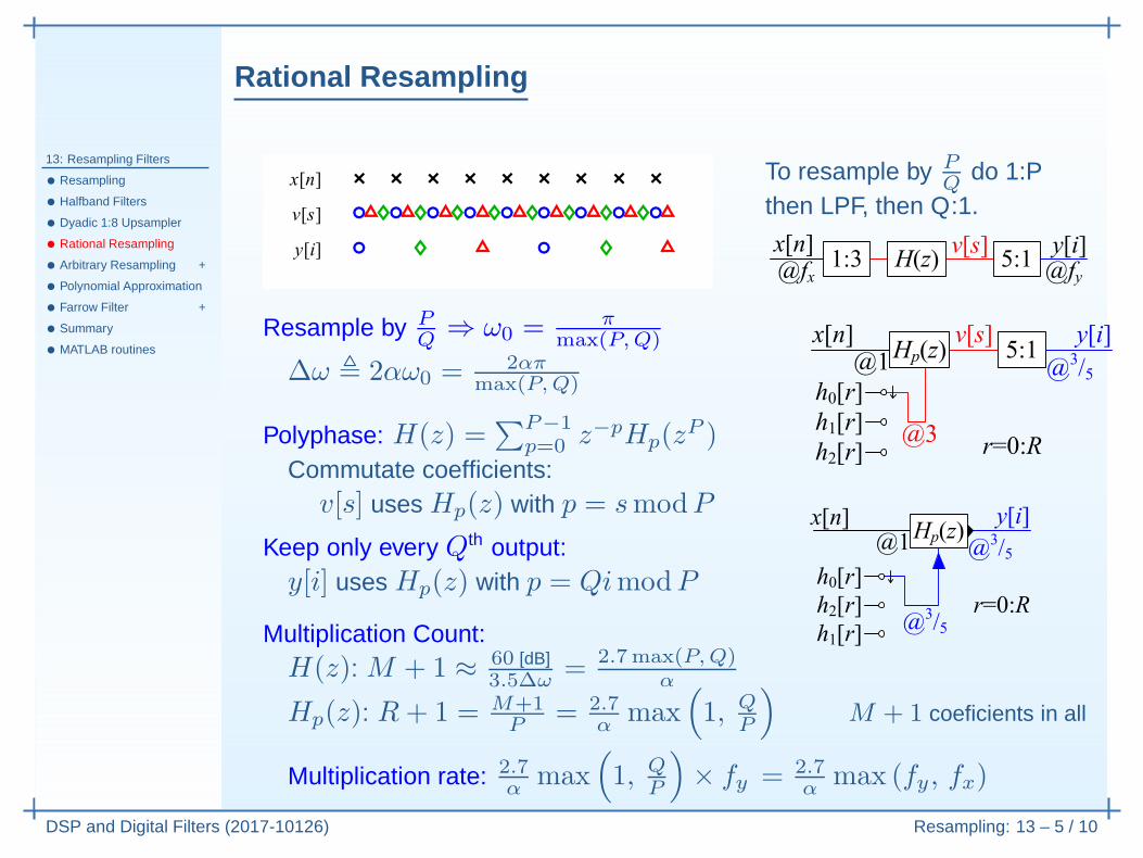
Rational Resampling
13: Resampling Filters
• Resampling
• Halfband Filters
• Dyadic 1:8 Upsampler
• Rational Resampling
• Arbitrary Resampling +
• Polynomial Approximation
• Farrow Filter +
• Summary
• MATLAB routines
DSP and Digital Filters (2017-10126) Resampling: 13 – 5 / 10
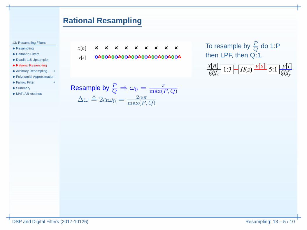
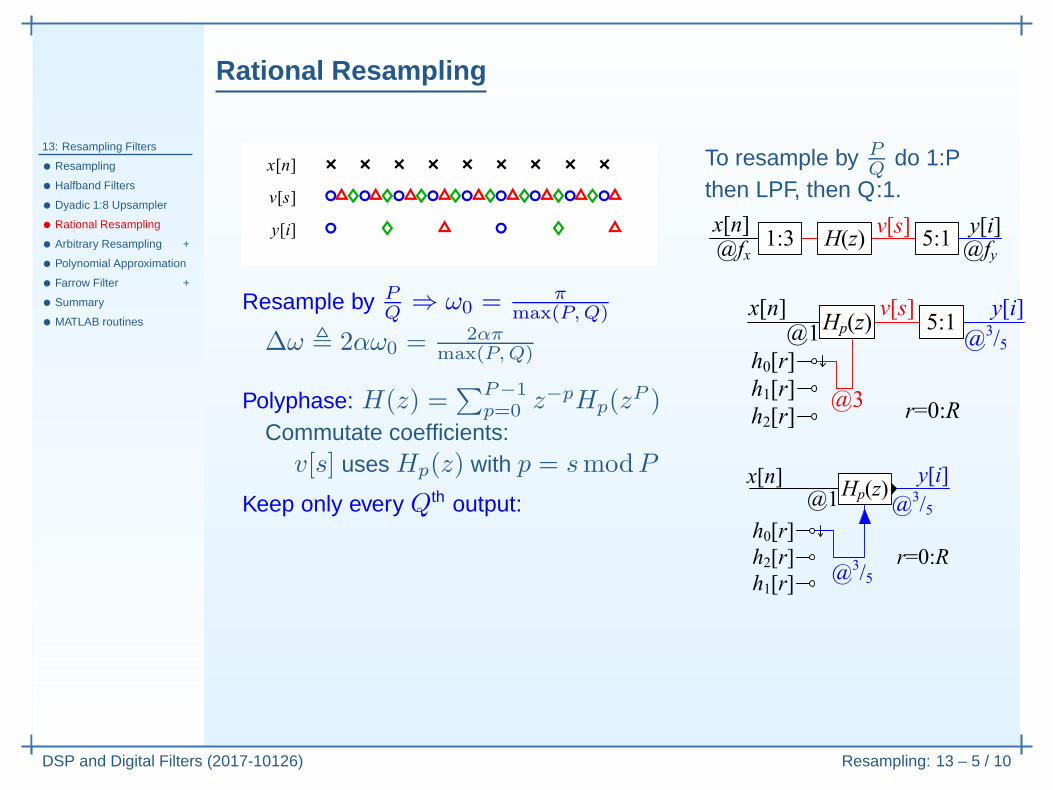
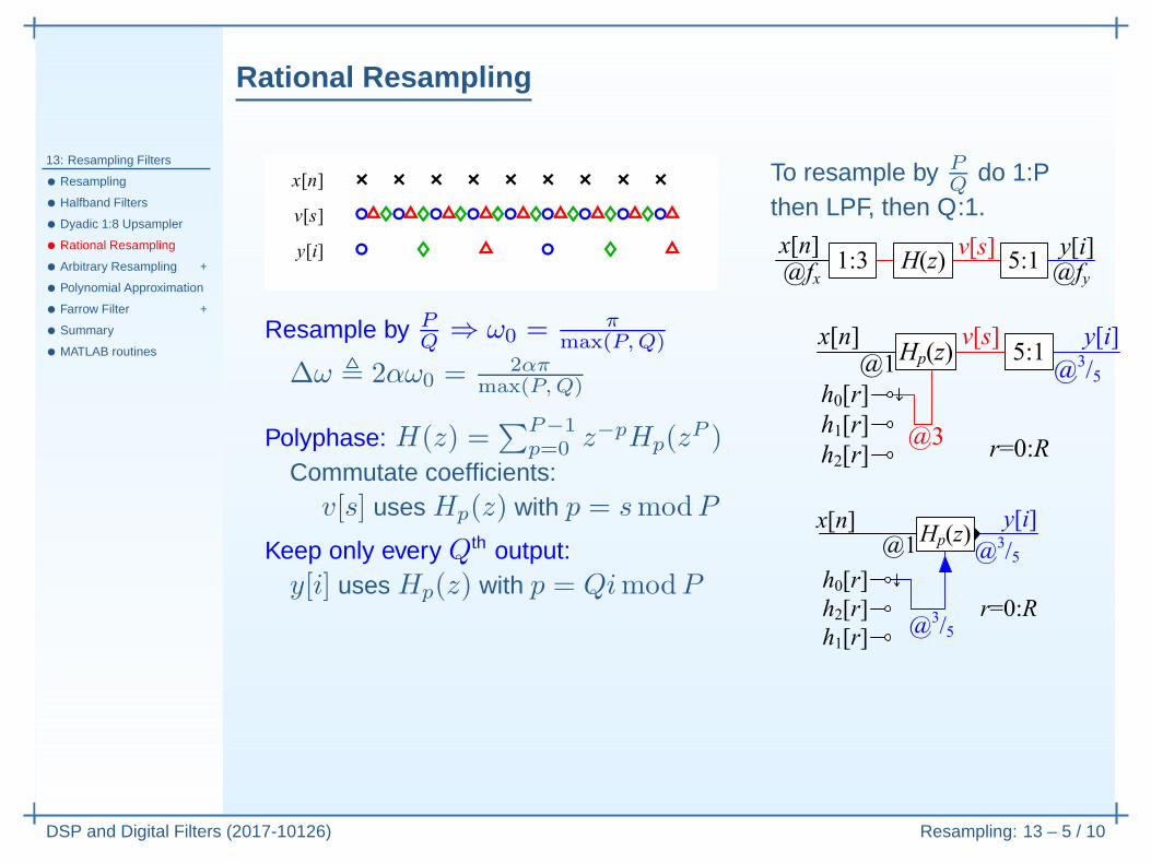
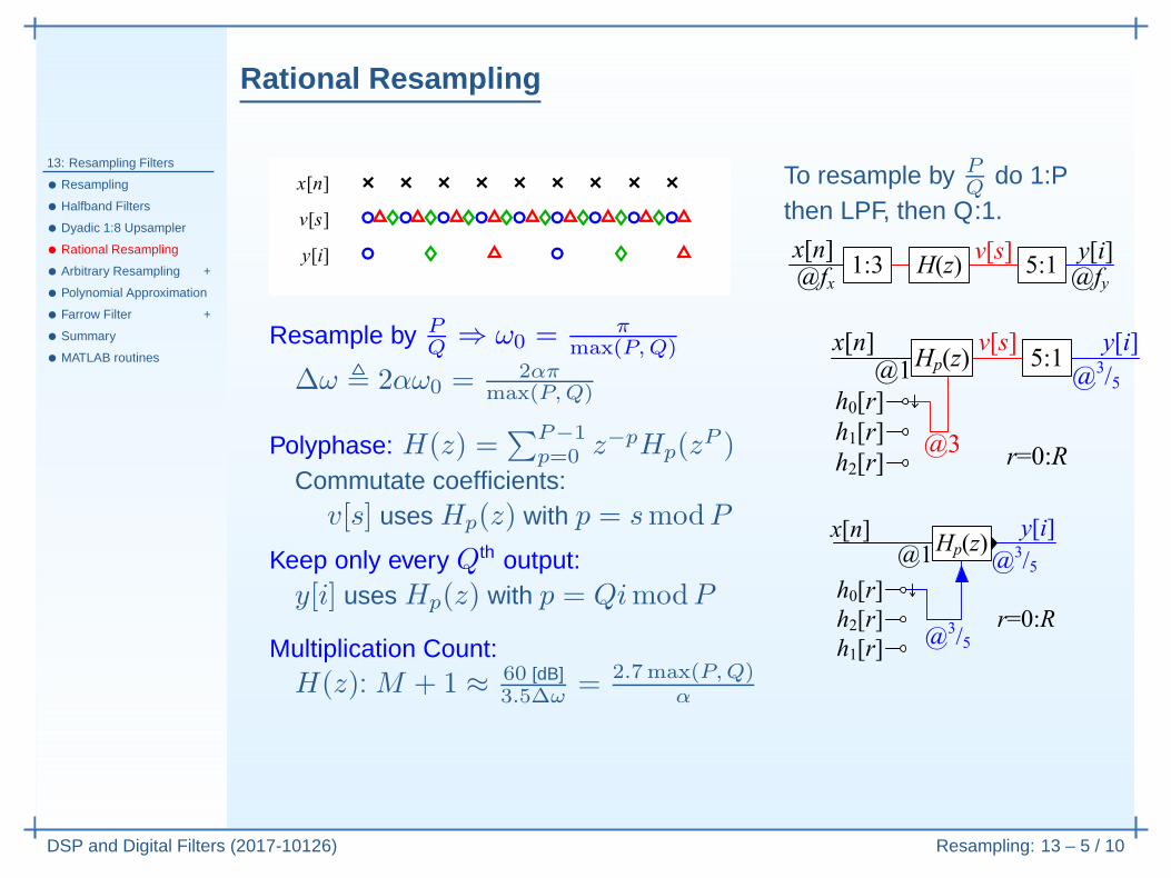
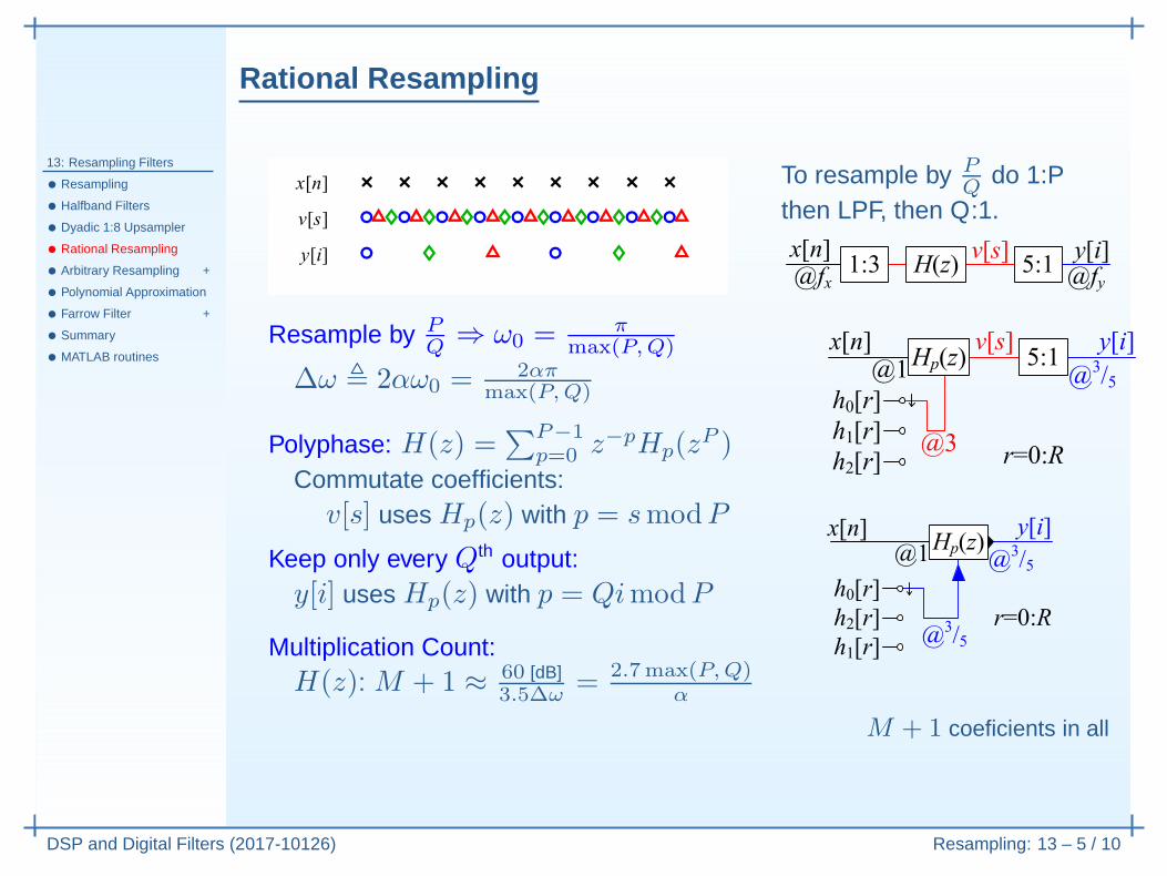
To resample by PQ
do 1:Pthen LPF, then Q:1.
Rational Resampling
13: Resampling Filters
• Resampling
• Halfband Filters
• Dyadic 1:8 Upsampler
• Rational Resampling
• Arbitrary Resampling +
• Polynomial Approximation
• Farrow Filter +
• Summary
• MATLAB routines
DSP and Digital Filters (2017-10126) Resampling: 13 – 5 / 10
To resample by PQ
do 1:Pthen LPF, then Q:1.
Resample by PQ
⇒ ω0 = πmax(P,Q)
∆ω , 2αω0 = 2απmax(P,Q)
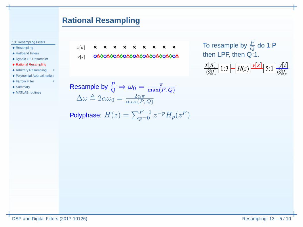
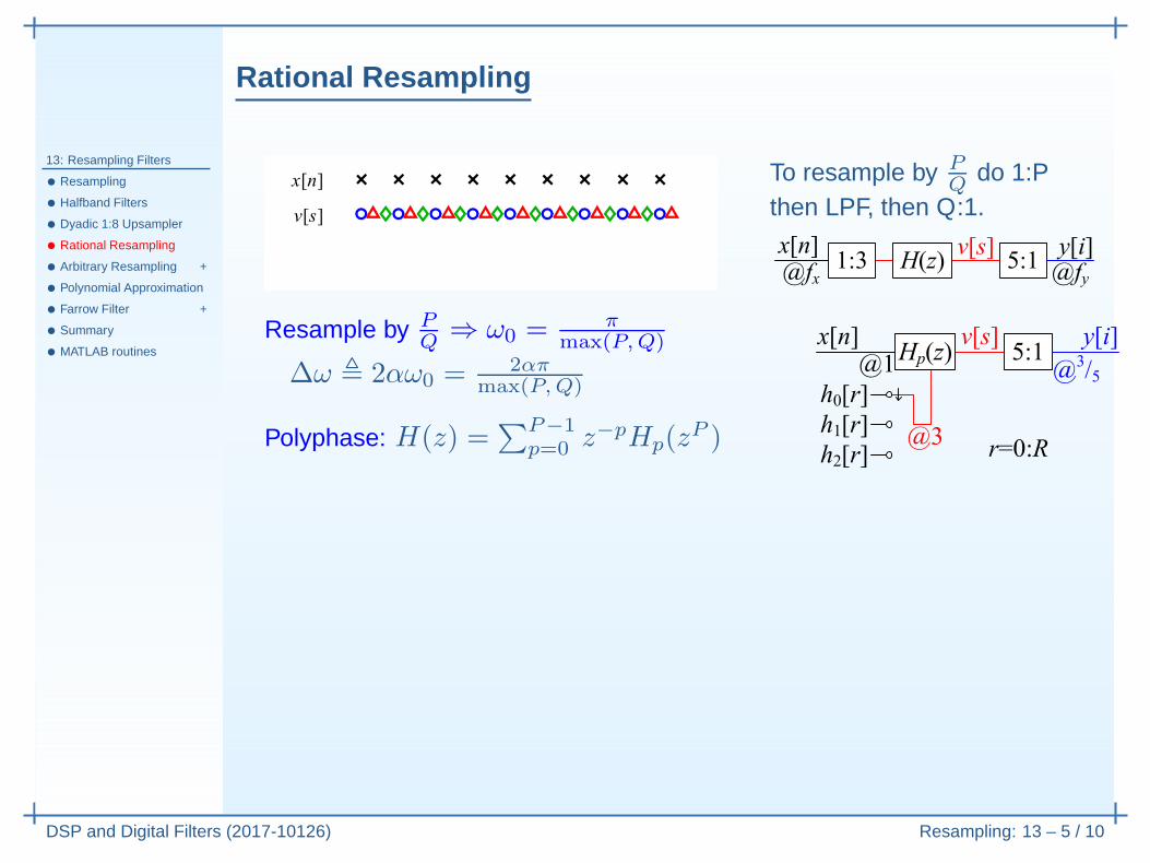
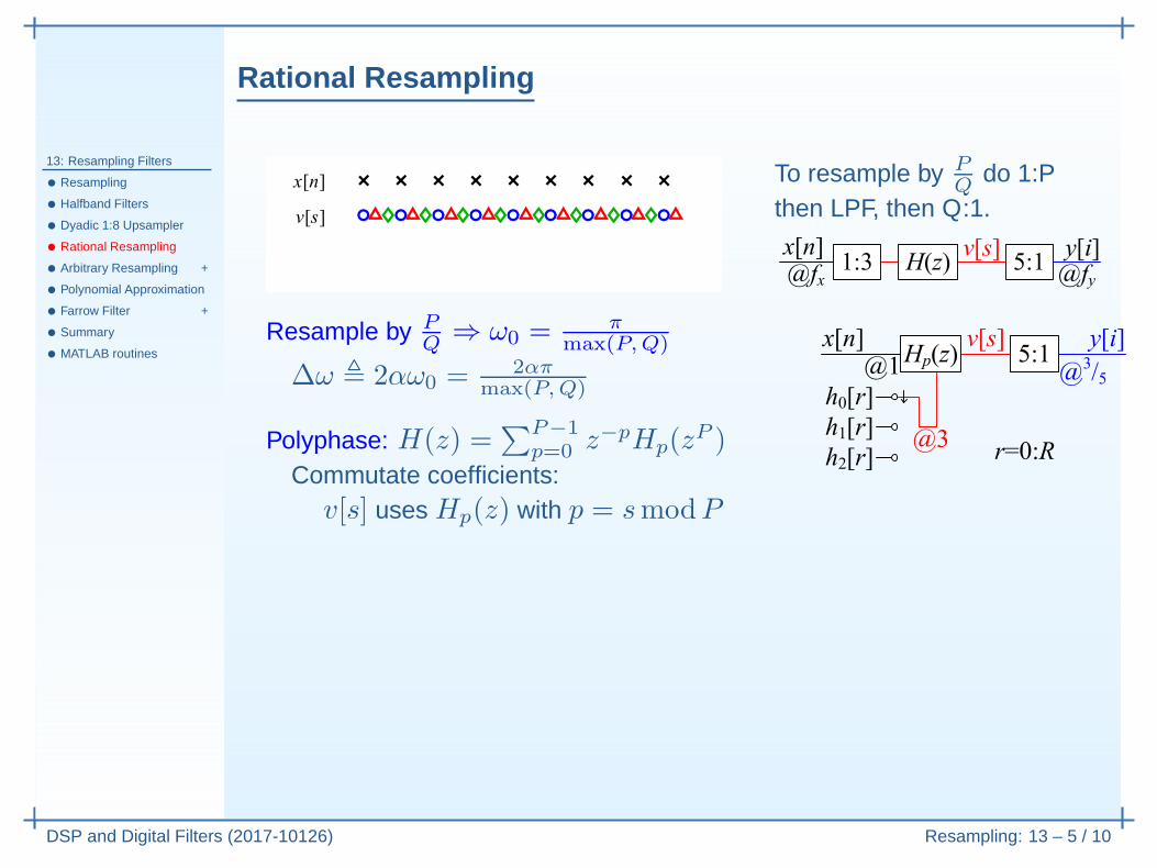
Polyphase: H(z) =∑P−1
p=0 z−pHp(zP )
Rational Resampling
13: Resampling Filters
• Resampling
• Halfband Filters
• Dyadic 1:8 Upsampler
• Rational Resampling
• Arbitrary Resampling +
• Polynomial Approximation
• Farrow Filter +
• Summary
• MATLAB routines
DSP and Digital Filters (2017-10126) Resampling: 13 – 5 / 10
To resample by PQ
do 1:Pthen LPF, then Q:1.
Resample by PQ
⇒ ω0 = πmax(P,Q)
∆ω , 2αω0 = 2απmax(P,Q)
Polyphase: H(z) =∑P−1
p=0 z−pHp(zP )
Commutate coefficients:v[s] uses Hp(z) with p = smodP
Keep only every Qth output:
Rational Resampling
13: Resampling Filters
• Resampling
• Halfband Filters
• Dyadic 1:8 Upsampler
• Rational Resampling
• Arbitrary Resampling +
• Polynomial Approximation
• Farrow Filter +
• Summary
• MATLAB routines
DSP and Digital Filters (2017-10126) Resampling: 13 – 5 / 10
To resample by PQ
do 1:Pthen LPF, then Q:1.
Resample by PQ
⇒ ω0 = πmax(P,Q)
∆ω , 2αω0 = 2απmax(P,Q)
Polyphase: H(z) =∑P−1
p=0 z−pHp(zP )
Commutate coefficients:v[s] uses Hp(z) with p = smodP
Keep only every Qth output:y[i] uses Hp(z) with p = QimodP
Multiplication Count:H(z): M + 1 ≈ 60 [dB]
3.5∆ω= 2.7max(P,Q)
α
M + 1 coeficients in all
Rational Resampling
13: Resampling Filters
• Resampling
• Halfband Filters
• Dyadic 1:8 Upsampler
• Rational Resampling
• Arbitrary Resampling +
• Polynomial Approximation
• Farrow Filter +
• Summary
• MATLAB routines
DSP and Digital Filters (2017-10126) Resampling: 13 – 5 / 10
To resample by PQ
do 1:Pthen LPF, then Q:1.
Resample by PQ
⇒ ω0 = πmax(P,Q)
∆ω , 2αω0 = 2απmax(P,Q)
Polyphase: H(z) =∑P−1
p=0 z−pHp(zP )
Commutate coefficients:v[s] uses Hp(z) with p = smodP
Keep only every Qth output:y[i] uses Hp(z) with p = QimodP
Multiplication Count:H(z): M + 1 ≈ 60 [dB]
3.5∆ω= 2.7max(P,Q)
α
Hp(z): R+ 1 = M+1P
= 2.7α
max(
1, Q
P
)
M + 1 coeficients in all
Multiplication rate: 2.7α
max(
1, QP
)
× fy
Rational Resampling
13: Resampling Filters
• Resampling
• Halfband Filters
• Dyadic 1:8 Upsampler
• Rational Resampling
• Arbitrary Resampling +
• Polynomial Approximation
• Farrow Filter +
• Summary
• MATLAB routines
DSP and Digital Filters (2017-10126) Resampling: 13 – 5 / 10
To resample by PQ
do 1:Pthen LPF, then Q:1.
Resample by PQ
⇒ ω0 = πmax(P,Q)
∆ω , 2αω0 = 2απmax(P,Q)
Polyphase: H(z) =∑P−1
p=0 z−pHp(zP )
Commutate coefficients:v[s] uses Hp(z) with p = smodP
Keep only every Qth output:y[i] uses Hp(z) with p = QimodP
Multiplication Count:H(z): M + 1 ≈ 60 [dB]
3.5∆ω= 2.7max(P,Q)
α
Hp(z): R+ 1 = M+1P
= 2.7α
max(
1, Q
P
)
M + 1 coeficients in all
Multiplication rate: 2.7α
max(
1, QP
)
× fy = 2.7α
max (fy, fx)
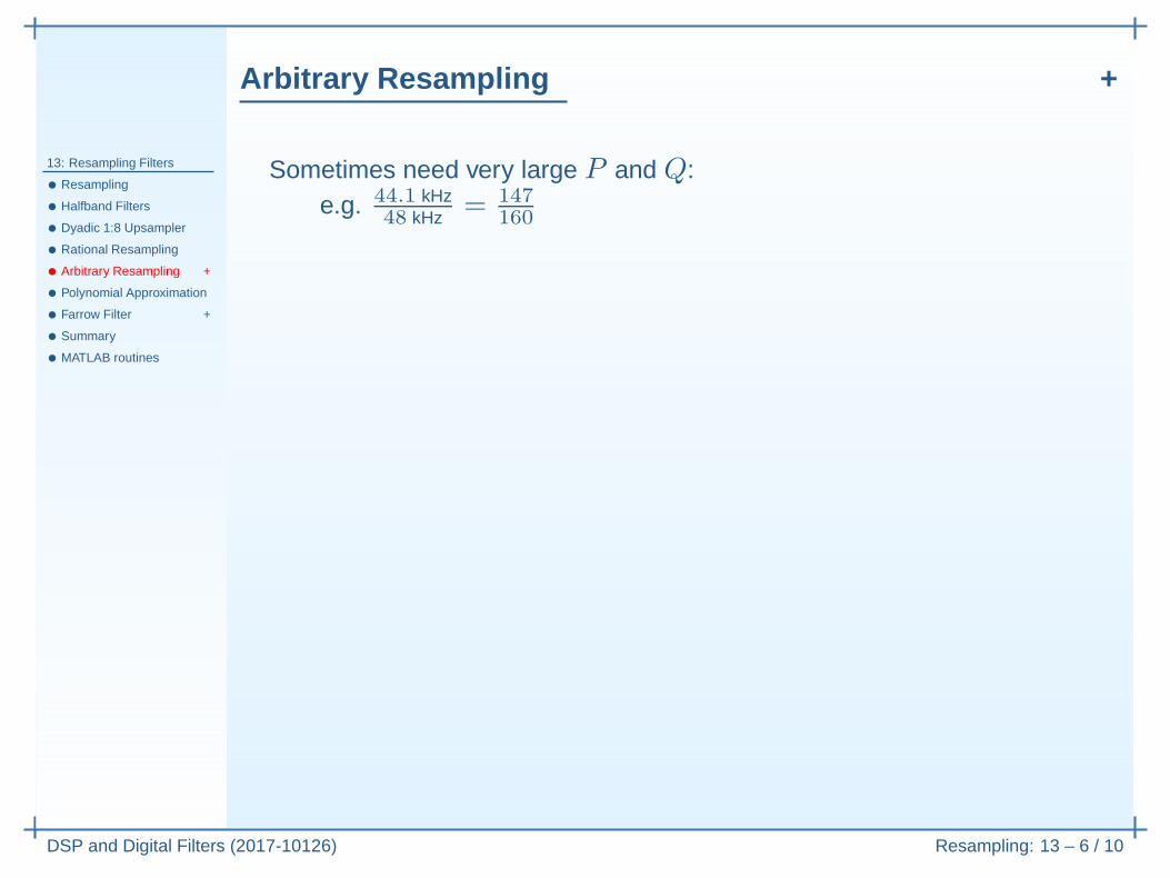
Arbitrary Resampling +
13: Resampling Filters
• Resampling
• Halfband Filters
• Dyadic 1:8 Upsampler
• Rational Resampling
• Arbitrary Resampling +
• Polynomial Approximation
• Farrow Filter +
• Summary
• MATLAB routines
DSP and Digital Filters (2017-10126) Resampling: 13 – 6 / 10
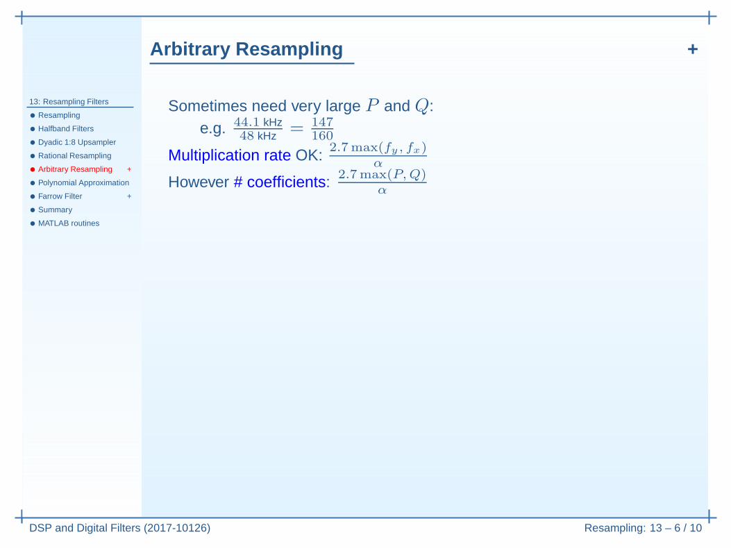
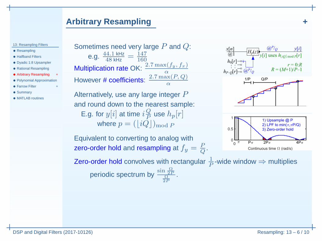
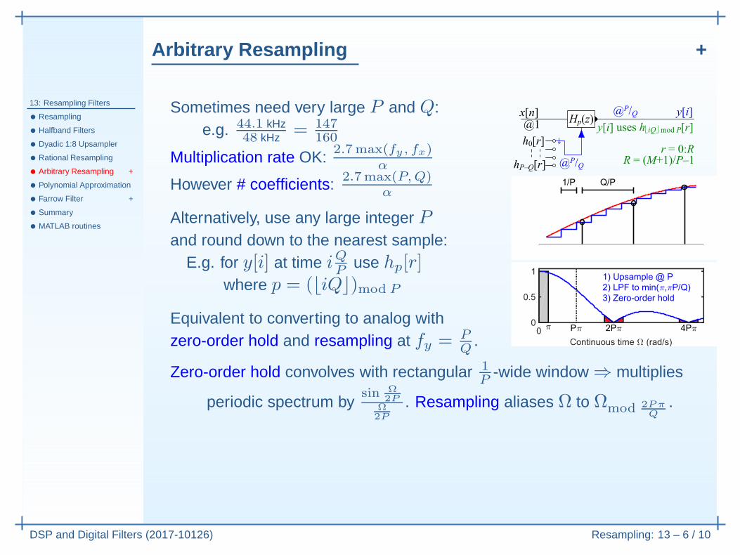
Sometimes need very large P and Q:e.g. 44.1 kHz
48 kHz = 147160
Arbitrary Resampling +
13: Resampling Filters
• Resampling
• Halfband Filters
• Dyadic 1:8 Upsampler
• Rational Resampling
• Arbitrary Resampling +
• Polynomial Approximation
• Farrow Filter +
• Summary
• MATLAB routines
DSP and Digital Filters (2017-10126) Resampling: 13 – 6 / 10
Sometimes need very large P and Q:e.g. 44.1 kHz
48 kHz = 147160
Multiplication rate OK:2.7max(fy, fx)
α
However # coefficients: 2.7max(P,Q)α
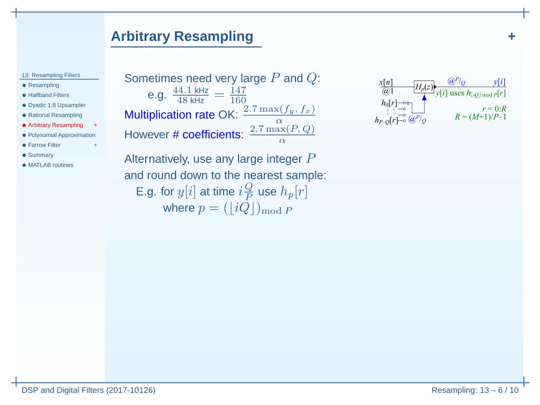
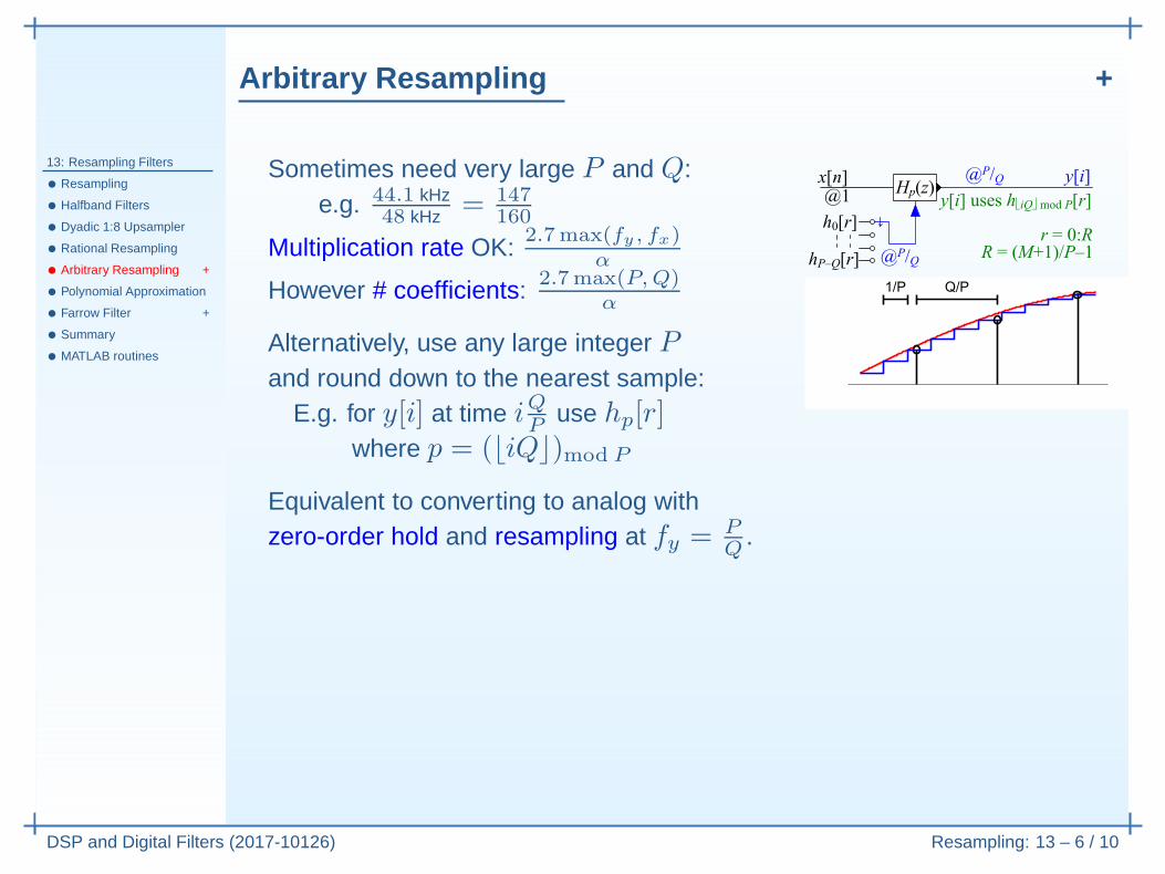
Alternatively, use any large integer Pand round down to the nearest sample:
E.g. for y[i] at time iQP
use hp[r]where p = (⌊iQ⌋)mod P
Arbitrary Resampling +
13: Resampling Filters
• Resampling
• Halfband Filters
• Dyadic 1:8 Upsampler
• Rational Resampling
• Arbitrary Resampling +
• Polynomial Approximation
• Farrow Filter +
• Summary
• MATLAB routines
DSP and Digital Filters (2017-10126) Resampling: 13 – 6 / 10
Sometimes need very large P and Q:e.g. 44.1 kHz
48 kHz = 147160
Multiplication rate OK:2.7max(fy, fx)
α
However # coefficients: 2.7max(P,Q)α
Alternatively, use any large integer Pand round down to the nearest sample:
E.g. for y[i] at time iQP
use hp[r]where p = (⌊iQ⌋)mod P
Equivalent to converting to analog withzero-order hold and resampling at fy = P
Q.
Zero-order hold convolves with rectangular 1P
-wide window ⇒ multiplies
periodic spectrum bysin Ω
2PΩ
2P
.
Arbitrary Resampling +
13: Resampling Filters
• Resampling
• Halfband Filters
• Dyadic 1:8 Upsampler
• Rational Resampling
• Arbitrary Resampling +
• Polynomial Approximation
• Farrow Filter +
• Summary
• MATLAB routines
DSP and Digital Filters (2017-10126) Resampling: 13 – 6 / 10
Sometimes need very large P and Q:e.g. 44.1 kHz
48 kHz = 147160
Multiplication rate OK:2.7max(fy, fx)
α
However # coefficients: 2.7max(P,Q)α
Alternatively, use any large integer Pand round down to the nearest sample:
E.g. for y[i] at time iQP
use hp[r]where p = (⌊iQ⌋)mod P
Equivalent to converting to analog withzero-order hold and resampling at fy = P
Q.
Zero-order hold convolves with rectangular 1P
-wide window ⇒ multiplies
periodic spectrum bysin Ω
2PΩ
2P
. Resampling aliases Ω to Ωmod 2PπQ
.
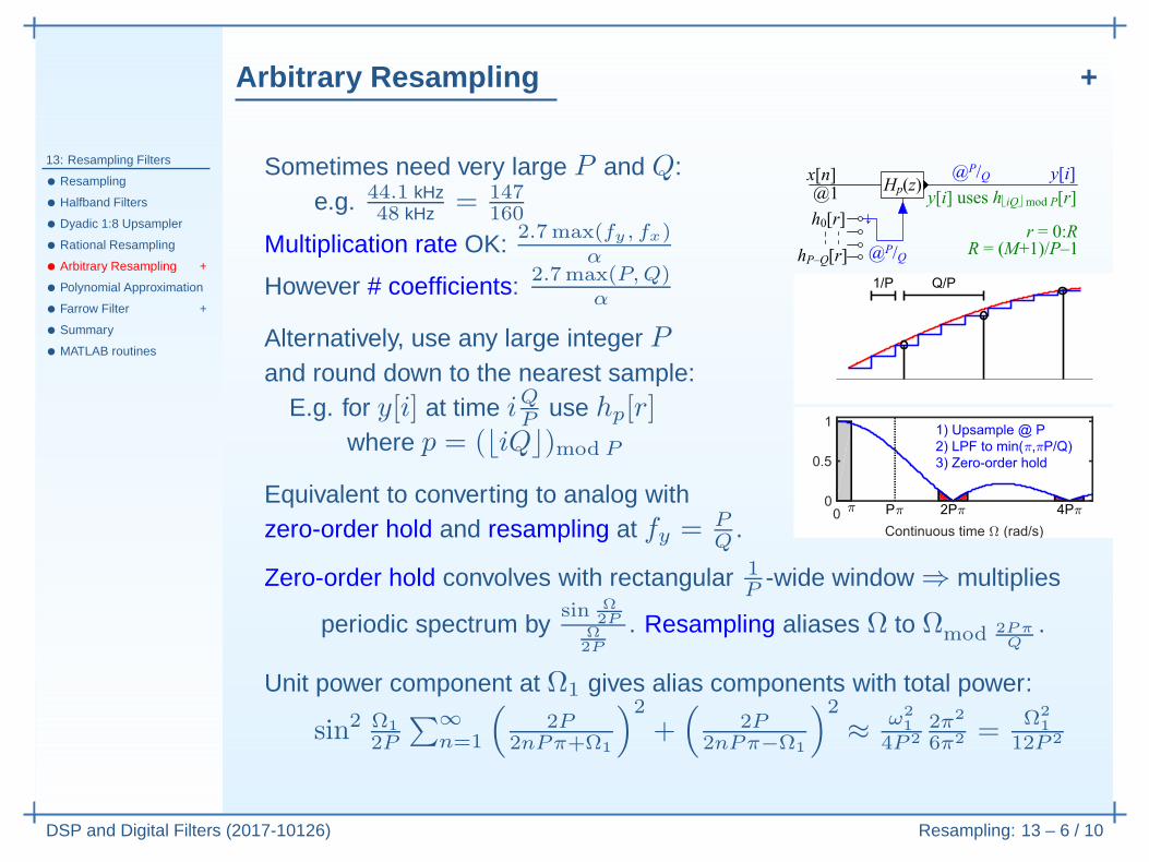
Unit power component at Ω1 gives alias components with total power:
sin2 Ω1
2P
∑
∞
n=1
(
2P2nPπ+Ω1
)2
+(
2P2nPπ−Ω1
)2
≈ω2
1
4P 2
2π2
6π2 =Ω2
1
12P 2
Arbitrary Resampling +
13: Resampling Filters
• Resampling
• Halfband Filters
• Dyadic 1:8 Upsampler
• Rational Resampling
• Arbitrary Resampling +
• Polynomial Approximation
• Farrow Filter +
• Summary
• MATLAB routines
DSP and Digital Filters (2017-10126) Resampling: 13 – 6 / 10
Sometimes need very large P and Q:e.g. 44.1 kHz
48 kHz = 147160
Multiplication rate OK:2.7max(fy, fx)
α
However # coefficients: 2.7max(P,Q)α
Alternatively, use any large integer Pand round down to the nearest sample:
E.g. for y[i] at time iQP
use hp[r]where p = (⌊iQ⌋)mod P
Equivalent to converting to analog withzero-order hold and resampling at fy = P
Q.
Zero-order hold convolves with rectangular 1P
-wide window ⇒ multiplies
periodic spectrum bysin Ω
2PΩ
2P
. Resampling aliases Ω to Ωmod 2PπQ
.
Unit power component at Ω1 gives alias components with total power:
sin2 Ω1
2P
∑
∞
n=1
(
2P2nPπ+Ω1
)2
+(
2P2nPπ−Ω1
)2
≈ω2
1
4P 2
2π2
6π2 =Ω2
1
12P 2
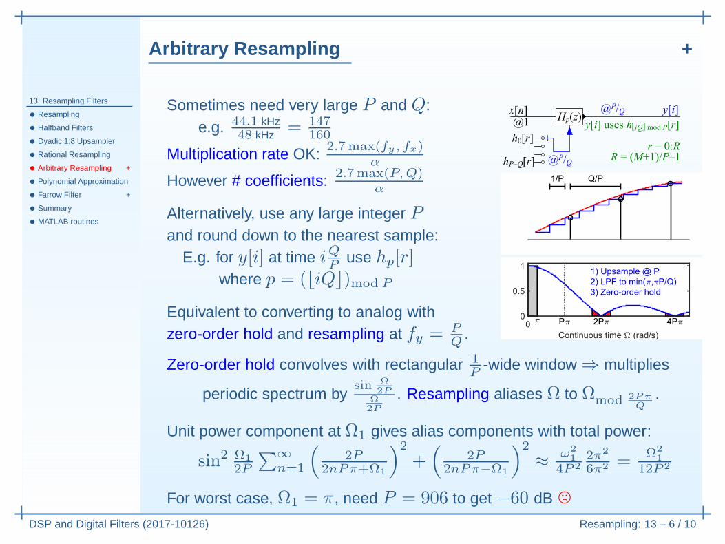
For worst case, Ω1 = π, need P = 906 to get −60 dB /
Polynomial Approximation
13: Resampling Filters
• Resampling
• Halfband Filters
• Dyadic 1:8 Upsampler
• Rational Resampling
• Arbitrary Resampling +
• Polynomial Approximation
• Farrow Filter +
• Summary
• MATLAB routines
DSP and Digital Filters (2017-10126) Resampling: 13 – 7 / 10
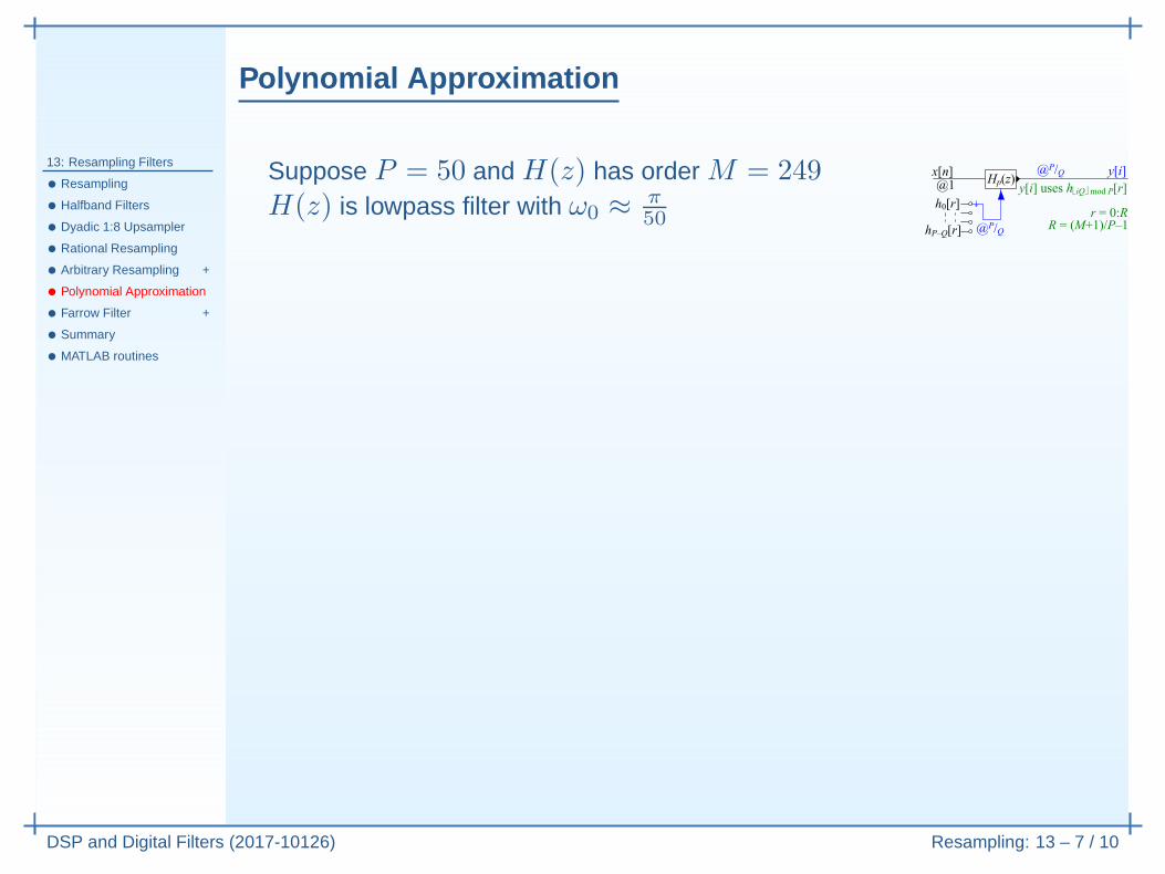
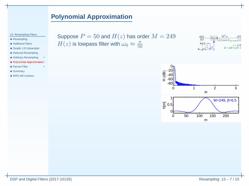
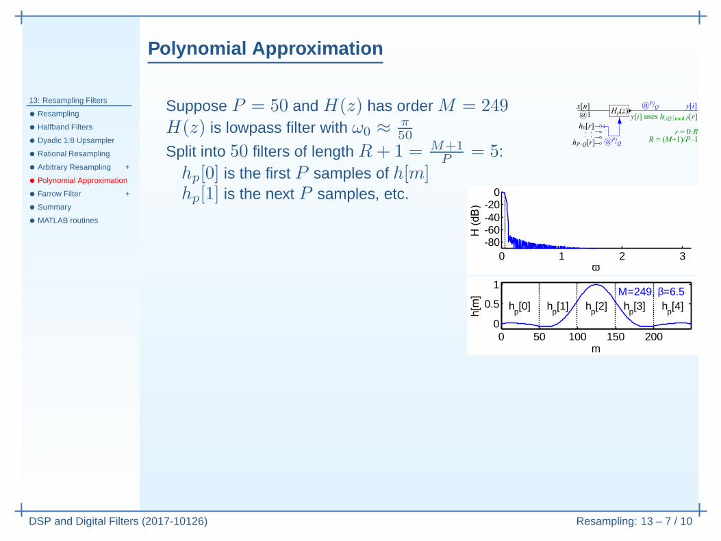
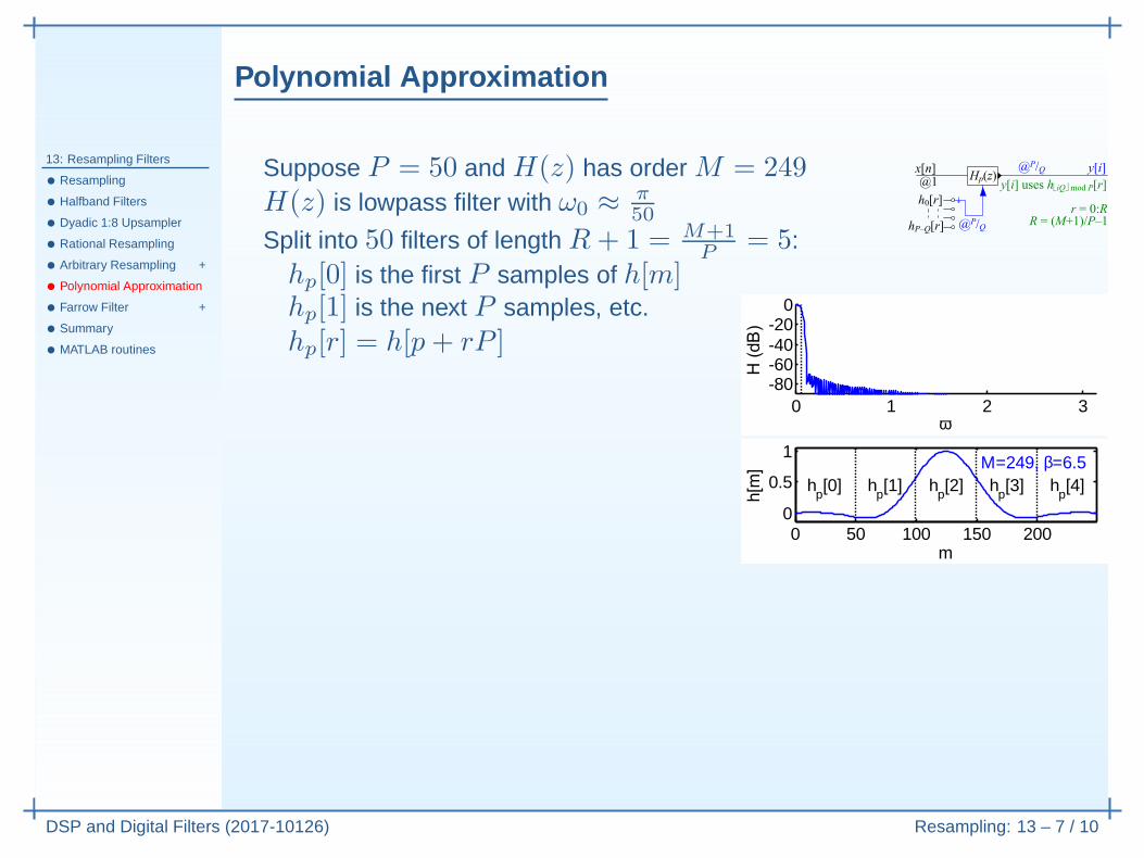
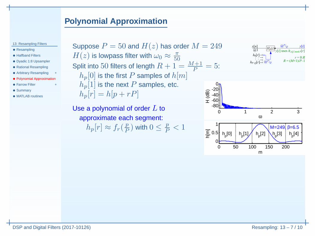
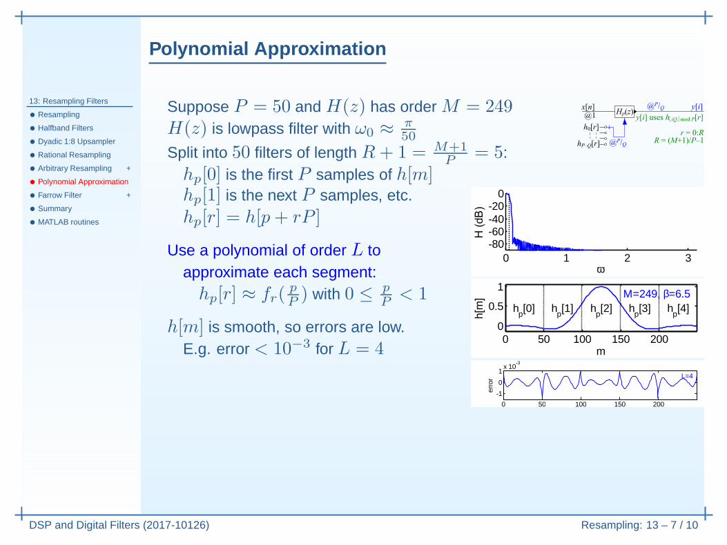
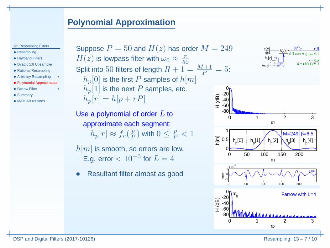
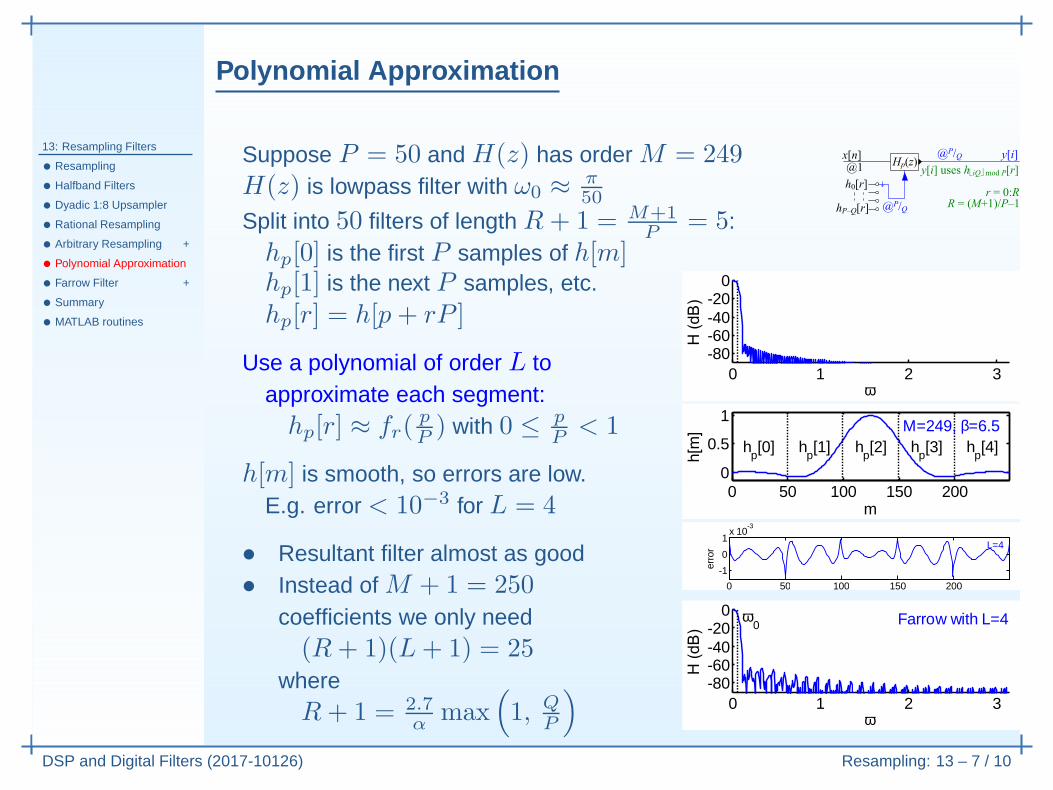
Suppose P = 50 and H(z) has order M = 249H(z) is lowpass filter with ω0 ≈ π
50
0 0 0 0 0
Polynomial Approximation
13: Resampling Filters
• Resampling
• Halfband Filters
• Dyadic 1:8 Upsampler
• Rational Resampling
• Arbitrary Resampling +
• Polynomial Approximation
• Farrow Filter +
• Summary
• MATLAB routines
DSP and Digital Filters (2017-10126) Resampling: 13 – 7 / 10
Suppose P = 50 and H(z) has order M = 249H(z) is lowpass filter with ω0 ≈ π
50
0 1 2 3-80-60-40-20
0
ω
0 50 100 150 2000
0.5
1M=249, β=6.5
m
0 0 0 0 0
Polynomial Approximation
13: Resampling Filters
• Resampling
• Halfband Filters
• Dyadic 1:8 Upsampler
• Rational Resampling
• Arbitrary Resampling +
• Polynomial Approximation
• Farrow Filter +
• Summary
• MATLAB routines
DSP and Digital Filters (2017-10126) Resampling: 13 – 7 / 10
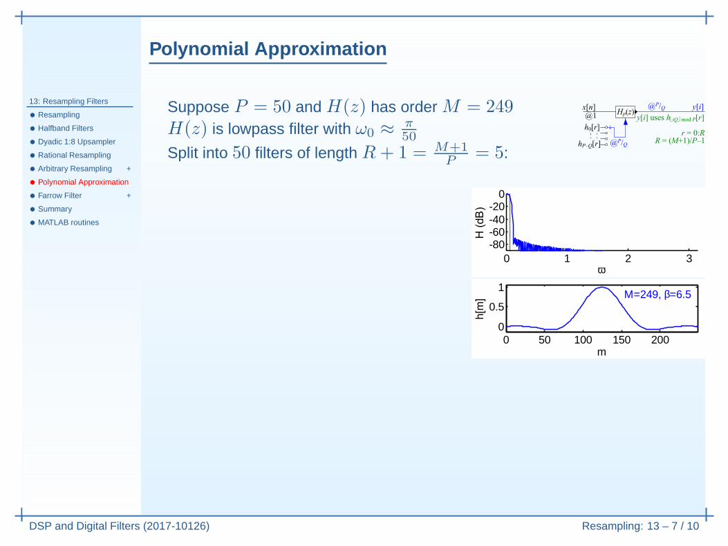
Suppose P = 50 and H(z) has order M = 249H(z) is lowpass filter with ω0 ≈ π
50
Split into 50 filters of length R + 1 = M+1P
= 5:
0 1 2 3-80-60-40-20
0
ω
0 50 100 150 2000
0.5
1M=249, β=6.5
m
0 0 0 0 0
Polynomial Approximation
13: Resampling Filters
• Resampling
• Halfband Filters
• Dyadic 1:8 Upsampler
• Rational Resampling
• Arbitrary Resampling +
• Polynomial Approximation
• Farrow Filter +
• Summary
• MATLAB routines
DSP and Digital Filters (2017-10126) Resampling: 13 – 7 / 10
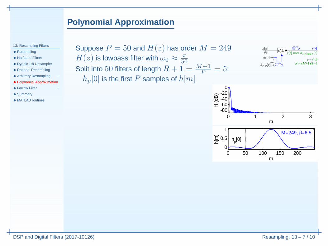
Suppose P = 50 and H(z) has order M = 249H(z) is lowpass filter with ω0 ≈ π
50
Split into 50 filters of length R + 1 = M+1P
= 5:hp[0] is the first P samples of h[m]
0 1 2 3-80-60-40-20
0
ω
0 50 100 150 2000
0.5
1
hp[0]
M=249, β=6.5
m
0 0 0 0 0
Polynomial Approximation
13: Resampling Filters
• Resampling
• Halfband Filters
• Dyadic 1:8 Upsampler
• Rational Resampling
• Arbitrary Resampling +
• Polynomial Approximation
• Farrow Filter +
• Summary
• MATLAB routines
DSP and Digital Filters (2017-10126) Resampling: 13 – 7 / 10
Suppose P = 50 and H(z) has order M = 249H(z) is lowpass filter with ω0 ≈ π
50
Split into 50 filters of length R + 1 = M+1P
= 5:hp[0] is the first P samples of h[m]hp[1] is the next P samples, etc.
0 1 2 3-80-60-40-20
0
ω
0 50 100 150 2000
0.5
1
hp[0] h
p[1] h
p[2] h
p[3] h
p[4]
M=249, β=6.5
m
0 0 0 0 0
Polynomial Approximation
13: Resampling Filters
• Resampling
• Halfband Filters
• Dyadic 1:8 Upsampler
• Rational Resampling
• Arbitrary Resampling +
• Polynomial Approximation
• Farrow Filter +
• Summary
• MATLAB routines
DSP and Digital Filters (2017-10126) Resampling: 13 – 7 / 10
Suppose P = 50 and H(z) has order M = 249H(z) is lowpass filter with ω0 ≈ π
50
Split into 50 filters of length R + 1 = M+1P
= 5:hp[0] is the first P samples of h[m]hp[1] is the next P samples, etc.hp[r] = h[p+ rP ]
Use a polynomial of order L toapproximate each segment:hp[r] ≈ fr(
pP) with 0 ≤ p
P< 1
h[m] is smooth, so errors are low.E.g. error < 10−3 for L = 4
0 1 2 3-80-60-40-20
0
ω
0 50 100 150 2000
0.5
1
hp[0] h
p[1] h
p[2] h
p[3] h
p[4]
M=249, β=6.5
m
0 50 100 150 200
-1
0
1x 10
-3
L=4
erro
r
Polynomial Approximation
13: Resampling Filters
• Resampling
• Halfband Filters
• Dyadic 1:8 Upsampler
• Rational Resampling
• Arbitrary Resampling +
• Polynomial Approximation
• Farrow Filter +
• Summary
• MATLAB routines
DSP and Digital Filters (2017-10126) Resampling: 13 – 7 / 10
Suppose P = 50 and H(z) has order M = 249H(z) is lowpass filter with ω0 ≈ π
50
Split into 50 filters of length R + 1 = M+1P
= 5:hp[0] is the first P samples of h[m]hp[1] is the next P samples, etc.hp[r] = h[p+ rP ]
Use a polynomial of order L toapproximate each segment:hp[r] ≈ fr(
pP) with 0 ≤ p
P< 1
h[m] is smooth, so errors are low.E.g. error < 10−3 for L = 4
• Resultant filter almost as good
0 1 2 3-80-60-40-20
0
ω
0 50 100 150 2000
0.5
1
hp[0] h
p[1] h
p[2] h
p[3] h
p[4]
M=249, β=6.5
m
0 50 100 150 200
-1
0
1x 10
-3
L=4
erro
r0 1 2 3
-80-60-40-20
0 Farrow with L=4
ω
ω0
Polynomial Approximation
13: Resampling Filters
• Resampling
• Halfband Filters
• Dyadic 1:8 Upsampler
• Rational Resampling
• Arbitrary Resampling +
• Polynomial Approximation
• Farrow Filter +
• Summary
• MATLAB routines
DSP and Digital Filters (2017-10126) Resampling: 13 – 7 / 10
Suppose P = 50 and H(z) has order M = 249H(z) is lowpass filter with ω0 ≈ π
50
Split into 50 filters of length R + 1 = M+1P
= 5:hp[0] is the first P samples of h[m]hp[1] is the next P samples, etc.hp[r] = h[p+ rP ]
Use a polynomial of order L toapproximate each segment:hp[r] ≈ fr(
pP) with 0 ≤ p
P< 1
h[m] is smooth, so errors are low.E.g. error < 10−3 for L = 4
• Resultant filter almost as good• Instead of M + 1 = 250
coefficients we only need(R+ 1)(L+ 1) = 25
whereR+ 1 = 2.7
αmax
(
1, Q
P
)
0 1 2 3-80-60-40-20
0
ω
0 50 100 150 2000
0.5
1
hp[0] h
p[1] h
p[2] h
p[3] h
p[4]
M=249, β=6.5
m
0 50 100 150 200
-1
0
1x 10
-3
L=4
erro
r0 1 2 3
-80-60-40-20
0 Farrow with L=4
ω
ω0
Farrow Filter +
13: Resampling Filters
• Resampling
• Halfband Filters
• Dyadic 1:8 Upsampler
• Rational Resampling
• Arbitrary Resampling +
• Polynomial Approximation
• Farrow Filter +
• Summary
• MATLAB routines
DSP and Digital Filters (2017-10126) Resampling: 13 – 8 / 10
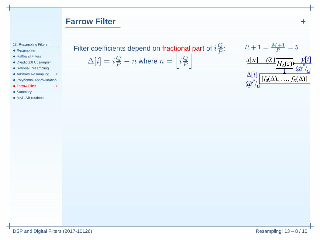
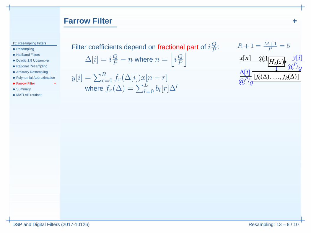
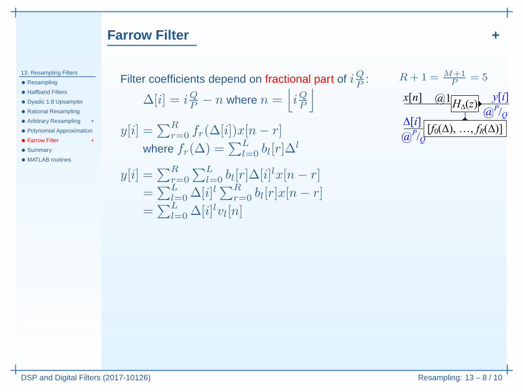
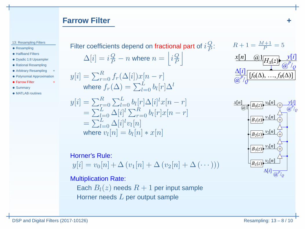
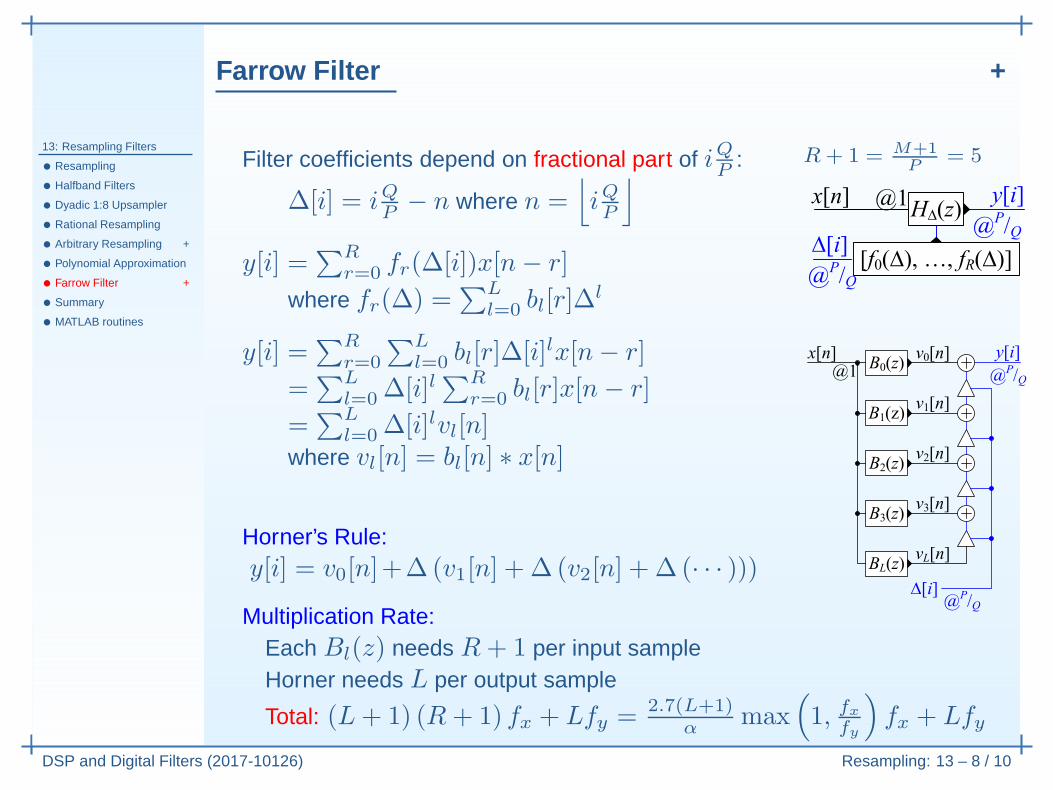
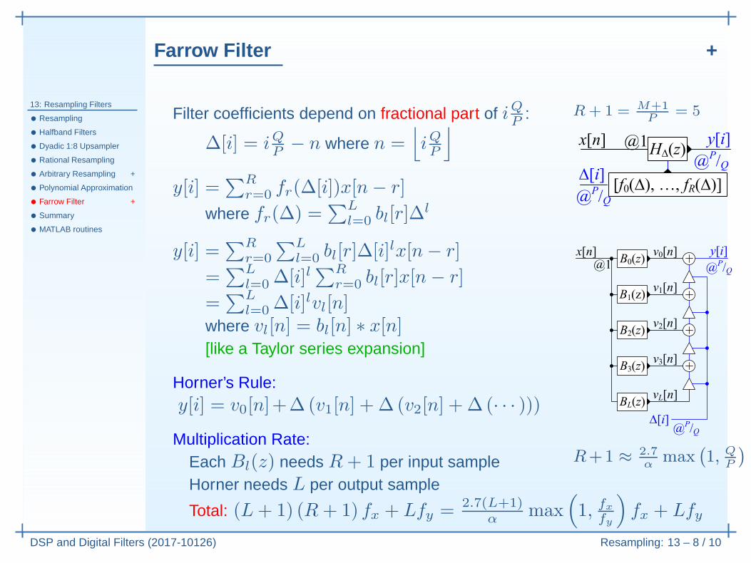
Filter coefficients depend on fractional part of iQP
:
∆[i] = iQP− n where n =
⌊
iQP
⌋
R+ 1 =M+1
P= 5
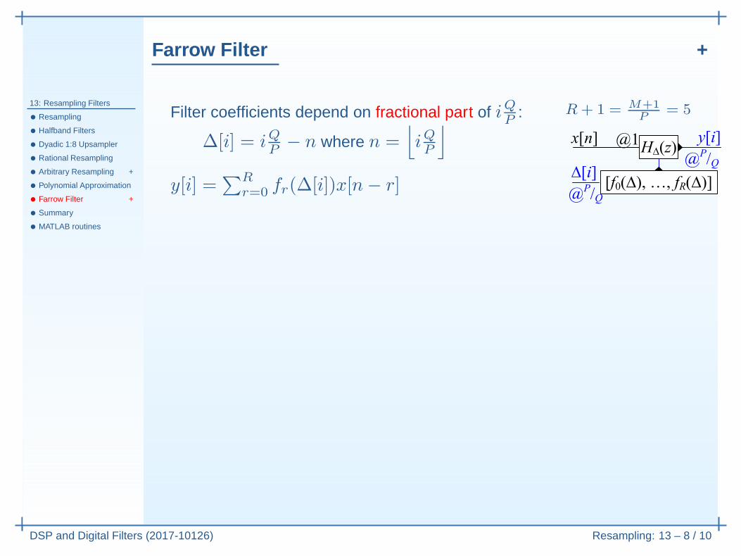
Farrow Filter +
13: Resampling Filters
• Resampling
• Halfband Filters
• Dyadic 1:8 Upsampler
• Rational Resampling
• Arbitrary Resampling +
• Polynomial Approximation
• Farrow Filter +
• Summary
• MATLAB routines
DSP and Digital Filters (2017-10126) Resampling: 13 – 8 / 10
Filter coefficients depend on fractional part of iQP
:
∆[i] = iQP− n where n =
⌊
iQP
⌋
y[i] =∑R
r=0 fr(∆[i])x[n− r]
R+ 1 =M+1
P= 5
Farrow Filter +
13: Resampling Filters
• Resampling
• Halfband Filters
• Dyadic 1:8 Upsampler
• Rational Resampling
• Arbitrary Resampling +
• Polynomial Approximation
• Farrow Filter +
• Summary
• MATLAB routines
DSP and Digital Filters (2017-10126) Resampling: 13 – 8 / 10
Filter coefficients depend on fractional part of iQP
:
∆[i] = iQP− n where n =
⌊
iQP
⌋
y[i] =∑R
r=0 fr(∆[i])x[n− r]
where fr(∆) =∑L
l=0 bl[r]∆l
y[i] =∑R
r=0
∑L
l=0 bl[r]∆[i]lx[n− r]
R+ 1 =M+1
P= 5
Farrow Filter +
13: Resampling Filters
• Resampling
• Halfband Filters
• Dyadic 1:8 Upsampler
• Rational Resampling
• Arbitrary Resampling +
• Polynomial Approximation
• Farrow Filter +
• Summary
• MATLAB routines
DSP and Digital Filters (2017-10126) Resampling: 13 – 8 / 10
Filter coefficients depend on fractional part of iQP
:
∆[i] = iQP− n where n =
⌊
iQP
⌋
y[i] =∑R
r=0 fr(∆[i])x[n− r]
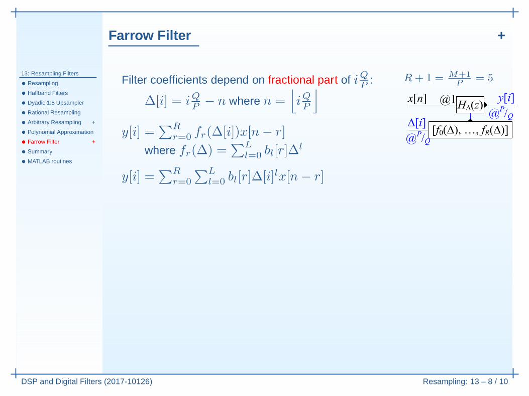
where fr(∆) =∑L
l=0 bl[r]∆l
y[i] =∑R
r=0
∑L
l=0 bl[r]∆[i]lx[n− r]
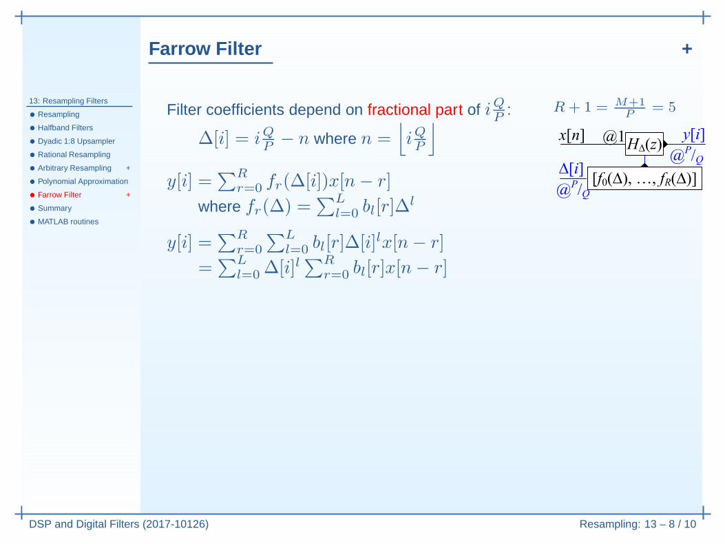
=∑L
l=0 ∆[i]l∑R
r=0 bl[r]x[n− r]
R+ 1 =M+1
P= 5
Farrow Filter +
13: Resampling Filters
• Resampling
• Halfband Filters
• Dyadic 1:8 Upsampler
• Rational Resampling
• Arbitrary Resampling +
• Polynomial Approximation
• Farrow Filter +
• Summary
• MATLAB routines
DSP and Digital Filters (2017-10126) Resampling: 13 – 8 / 10
Filter coefficients depend on fractional part of iQP
:
∆[i] = iQP− n where n =
⌊
iQP
⌋
y[i] =∑R
r=0 fr(∆[i])x[n− r]
where fr(∆) =∑L
l=0 bl[r]∆l
y[i] =∑R
r=0
∑L
l=0 bl[r]∆[i]lx[n− r]
=∑L
l=0 ∆[i]l∑R
r=0 bl[r]x[n− r]
=∑L
l=0 ∆[i]lvl[n]
R+ 1 =M+1
P= 5
Farrow Filter +
13: Resampling Filters
• Resampling
• Halfband Filters
• Dyadic 1:8 Upsampler
• Rational Resampling
• Arbitrary Resampling +
• Polynomial Approximation
• Farrow Filter +
• Summary
• MATLAB routines
DSP and Digital Filters (2017-10126) Resampling: 13 – 8 / 10
Filter coefficients depend on fractional part of iQP
:
∆[i] = iQP− n where n =
⌊
iQP
⌋
y[i] =∑R
r=0 fr(∆[i])x[n− r]
where fr(∆) =∑L
l=0 bl[r]∆l
y[i] =∑R
r=0
∑L
l=0 bl[r]∆[i]lx[n− r]
=∑L
l=0 ∆[i]l∑R
r=0 bl[r]x[n− r]
=∑L
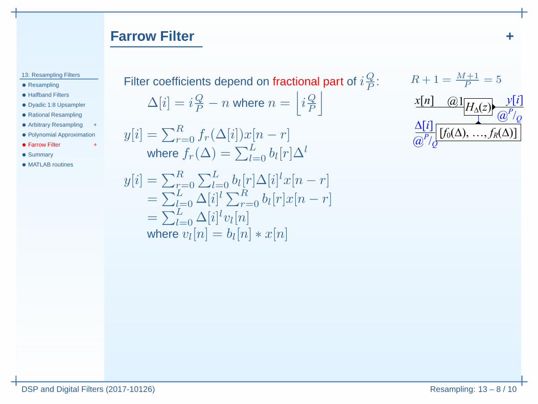
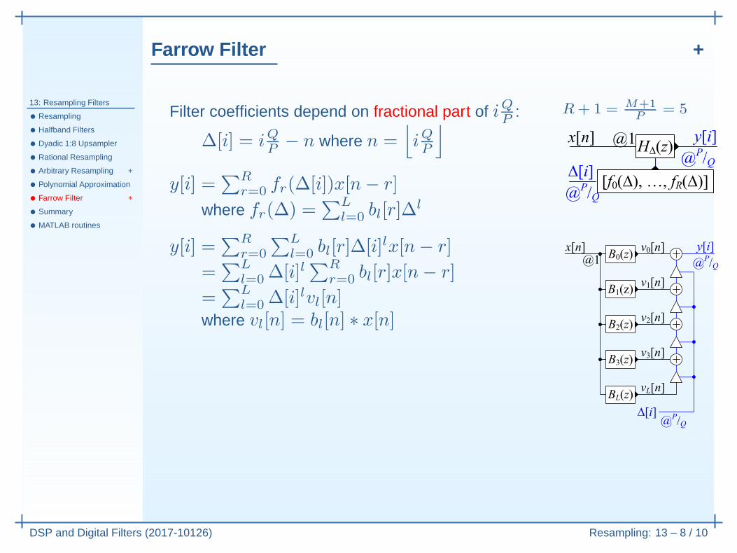
l=0 ∆[i]lvl[n]where vl[n] = bl[n] ∗ x[n]
R+ 1 =M+1
P= 5
Farrow Filter +
13: Resampling Filters
• Resampling
• Halfband Filters
• Dyadic 1:8 Upsampler
• Rational Resampling
• Arbitrary Resampling +
• Polynomial Approximation
• Farrow Filter +
• Summary
• MATLAB routines
DSP and Digital Filters (2017-10126) Resampling: 13 – 8 / 10
Filter coefficients depend on fractional part of iQP
:
∆[i] = iQP− n where n =
⌊
iQP
⌋
y[i] =∑R
r=0 fr(∆[i])x[n− r]
where fr(∆) =∑L
l=0 bl[r]∆l
y[i] =∑R
r=0
∑L
l=0 bl[r]∆[i]lx[n− r]
=∑L
l=0 ∆[i]l∑R
r=0 bl[r]x[n− r]
=∑L
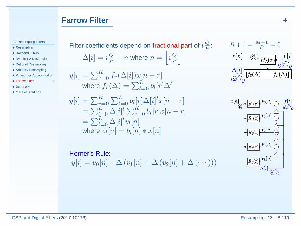
l=0 ∆[i]lvl[n]where vl[n] = bl[n] ∗ x[n]
Horner’s Rule:y[i] = v0[n]+∆ (v1[n] + ∆ (v2[n] + ∆ (· · · )))
R+ 1 =M+1
P= 5
Farrow Filter +
13: Resampling Filters
• Resampling
• Halfband Filters
• Dyadic 1:8 Upsampler
• Rational Resampling
• Arbitrary Resampling +
• Polynomial Approximation
• Farrow Filter +
• Summary
• MATLAB routines
DSP and Digital Filters (2017-10126) Resampling: 13 – 8 / 10
Filter coefficients depend on fractional part of iQP
:
∆[i] = iQP− n where n =
⌊
iQP
⌋
y[i] =∑R
r=0 fr(∆[i])x[n− r]
where fr(∆) =∑L
l=0 bl[r]∆l
y[i] =∑R
r=0
∑L
l=0 bl[r]∆[i]lx[n− r]
=∑L
l=0 ∆[i]l∑R
r=0 bl[r]x[n− r]
=∑L
l=0 ∆[i]lvl[n]where vl[n] = bl[n] ∗ x[n]
Horner’s Rule:y[i] = v0[n]+∆ (v1[n] + ∆ (v2[n] + ∆ (· · · )))
Multiplication Rate:Each Bl(z) needs R+ 1 per input sampleHorner needs L per output sample
R+ 1 =M+1
P= 5
Total: (L+ 1) (R + 1) fx + Lfy = 2.7(L+1)α
max(
1, fxfy
)
fx + Lfy
Farrow Filter +
13: Resampling Filters
• Resampling
• Halfband Filters
• Dyadic 1:8 Upsampler
• Rational Resampling
• Arbitrary Resampling +
• Polynomial Approximation
• Farrow Filter +
• Summary
• MATLAB routines
DSP and Digital Filters (2017-10126) Resampling: 13 – 8 / 10
Filter coefficients depend on fractional part of iQP
:
∆[i] = iQP− n where n =
⌊
iQP
⌋
y[i] =∑R
r=0 fr(∆[i])x[n− r]
where fr(∆) =∑L
l=0 bl[r]∆l
y[i] =∑R
r=0
∑L
l=0 bl[r]∆[i]lx[n− r]
=∑L
l=0 ∆[i]l∑R
r=0 bl[r]x[n− r]
=∑L
l=0 ∆[i]lvl[n]where vl[n] = bl[n] ∗ x[n][like a Taylor series expansion]
Horner’s Rule:y[i] = v0[n]+∆ (v1[n] + ∆ (v2[n] + ∆ (· · · )))
Multiplication Rate:Each Bl(z) needs R+ 1 per input sampleHorner needs L per output sample
R+ 1 =M+1
P= 5
R+1 ≈2.7
αmax
(
1,Q
P
)
Total: (L+ 1) (R + 1) fx + Lfy = 2.7(L+1)α
max(
1, fxfy
)
fx + Lfy
Summary
13: Resampling Filters
• Resampling
• Halfband Filters
• Dyadic 1:8 Upsampler
• Rational Resampling
• Arbitrary Resampling +
• Polynomial Approximation
• Farrow Filter +
• Summary
• MATLAB routines
DSP and Digital Filters (2017-10126) Resampling: 13 – 9 / 10
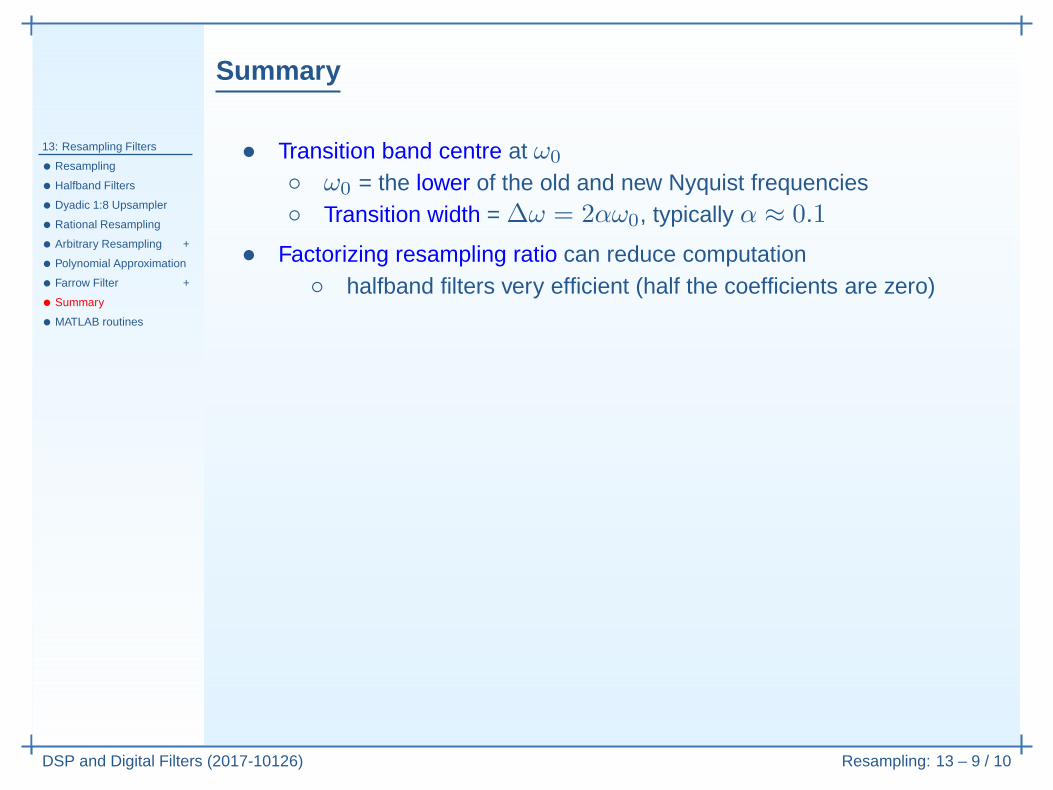
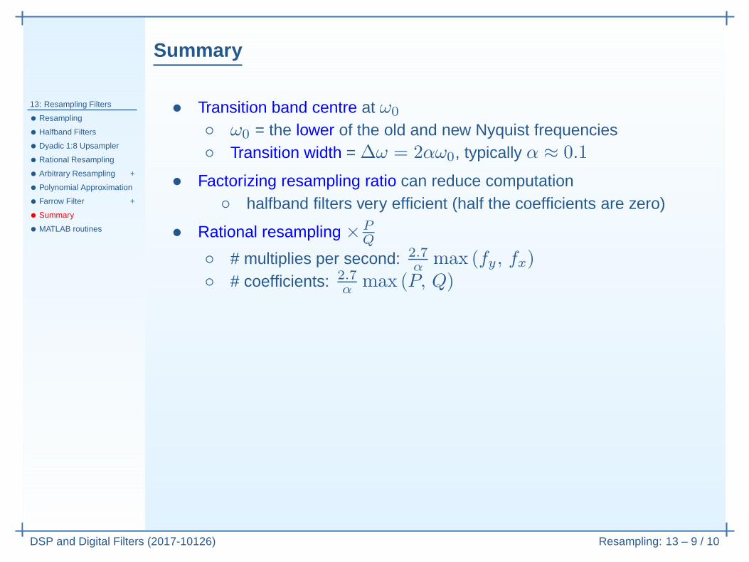
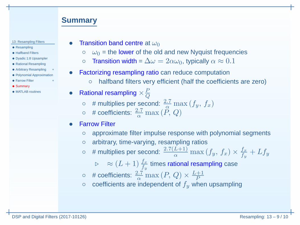
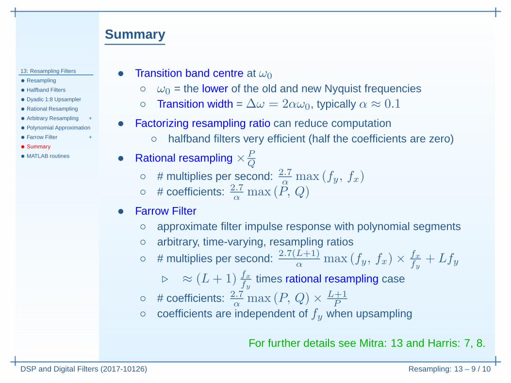
• Transition band centre at ω0
ω0 = the lower of the old and new Nyquist frequencies Transition width = ∆ω = 2αω0, typically α ≈ 0.1
Summary
13: Resampling Filters
• Resampling
• Halfband Filters
• Dyadic 1:8 Upsampler
• Rational Resampling
• Arbitrary Resampling +
• Polynomial Approximation
• Farrow Filter +
• Summary
• MATLAB routines
DSP and Digital Filters (2017-10126) Resampling: 13 – 9 / 10
• Transition band centre at ω0
ω0 = the lower of the old and new Nyquist frequencies Transition width = ∆ω = 2αω0, typically α ≈ 0.1
• Factorizing resampling ratio can reduce computation halfband filters very efficient (half the coefficients are zero)
• Rational resampling ×PQ
# multiplies per second: 2.7α
max (fy, fx) # coefficients: 2.7
αmax (P, Q)
• Farrow Filter approximate filter impulse response with polynomial segments arbitrary, time-varying, resampling ratios
# multiplies per second: 2.7(L+1)α
max (fy, fx)×fxfy
+ Lfy
⊲ ≈ (L+ 1) fxfy
times rational resampling case
# coefficients: 2.7α
max (P, Q)× L+1P
coefficients are independent of fy when upsampling
For further details see Mitra: 13 and Harris: 7, 8.
MATLAB routines
13: Resampling Filters
• Resampling
• Halfband Filters
• Dyadic 1:8 Upsampler
• Rational Resampling
• Arbitrary Resampling +
• Polynomial Approximation
• Farrow Filter +
• Summary
• MATLAB routines
DSP and Digital Filters (2017-10126) Resampling: 13 – 10 / 10
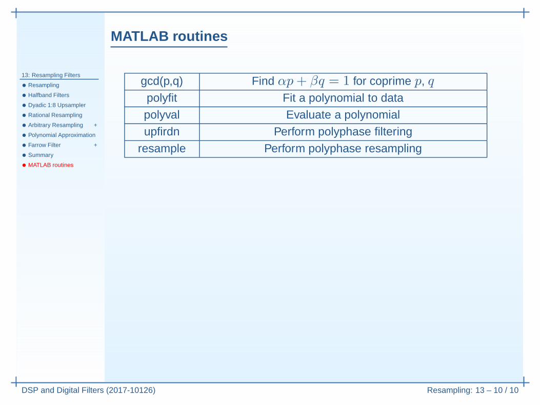
gcd(p,q) Find αp+ βq = 1 for coprime p, qpolyfit Fit a polynomial to datapolyval Evaluate a polynomialupfirdn Perform polyphase filtering
resample Perform polyphase resampling