applications of high resolution remote sensing in...
TRANSCRIPT
Rainforest CRCHeadquarters at James Cook University, Smithfield, Cairns
Postal address: PO Box 6811, Cairns, QLD 4870, AUSTRALIAPhone: (07) 4042 1246 Fax: (07) 4042 1247
Email: [email protected]://www.rainforest-crc.jcu.edu.au
The Cooperative Research Centre for Tropical Rainforest Ecology and Management (Rainforest CRC) is a research partnership involving the Commonwealth and Queensland State Governments, the Wet Tropics Management Authority, the tourism industry, Aboriginal groups, the CSIRO,
James Cook University, Griffith University and The University of Queensland.
Applications of HighResolution Remote Sensing
in Rainforest Ecologyand Management
David S. Gillieson,Tina J. Lawson and Les Searle
Cooperative Research Centre for Tropical Rainforest Ecology and Management
RESEARCH REPORT


APPLICATIONS OF HIGH RESOLUTION REMOTE SENSING IN RAINFOREST
ECOLOGY AND MANAGEMENT
David S. Gillieson, Tina J. Lawson and Les Searle School of Tropical Environment Studies and Geography,
James Cook University, Cairns
Established and supported under the
Australian Cooperative Research Centres Program
© Cooperative Research Centre for Tropical Rainforest Ecology and Management. ISBN 0 86443 770 6 This work is copyright. The Copyright Act 1968 permits fair dealing for study, research, news reporting, criticism or review. Selected passages, tables or diagrams may be reproduced for such purposes provided acknowledgment of the source is included. Major extracts of the entire document may not be reproduced by any process without written permission of the Chief Executive Officer, Cooperative Research Centre for Tropical Rainforest Ecology and Management. Published by the Cooperative Research Centre for Tropical Rainforest Ecology and Management. Further copies may be requested from the Cooperative Research Centre for Tropical Rainforest Ecology and Management, James Cook University, PO Box 6811, Cairns QLD 4870, Australia. This publication should be cited as: Gillieson, D., Lawson, T. and Searle, L. (2006). Applications of High Resolution Remote Sensing in Rainforest Ecology and Management. Cooperative Research Centre for Tropical Rainforest Ecology and Management. Rainforest CRC, Cairns (54 pp.). Cover Images © (Top) IKONOS-image of Smithfield region. Image: TESAG. (Centre) Riparian vegetation change in the Mossman Shire. Image: Tina Lawson / TESAG. (Bottom) Classified IKONOS-image of the McAllister Range, Smithfield. Image: TESAG. June 2006 Layout by B. Kuehn and S. Hogan For copies of this document, please visit www.rainforest-crc.jcu.edu.au

Applications of High Resolution Remote Sensing
i
ABSTRACT A new generation of satellite sensors has vastly improved spatial and spectral resolution, with additional radiometric resolution to 11-bit data (2048 grey levels). Repeat coverage is possible at 3-5 day intervals, making them ideal for assessing rapid environmental changes, such as fires and floods. Quickbird and IKONOS sensors have spatial resolutions of 0.6 to 1 m in panchromatic and 2.5 to 4 m (respectively) in multispectral mode. Spectrally, four bands from visible blue to near infra-red are available, with good separation and narrow bandwidth. For the first time we are thus able to resolve features down to the size of individual tree canopies. In this report we provide a number of examples using high resolution imagery to illustrate various methods of digital image analysis. All are drawn from research carried out since year 2000 in the Wet Tropics World Heritage Area under the auspices of the Cooperative Research Centre for Tropical Rainforest Ecology and Management (Rainforest CRC) in Cairns, North Queensland. Studies include the use of high resolution remote sensing for mapping weeds, dieback, forest fires and riparian vegetation change. In addition, we report on the use of high resolution imagery for mapping the canopy connectivity across roads. The challenges remaining for researchers are to evaluate new image classification methodologies, such as object oriented classifiers, to rainforest environments and to further refine the models that relate forest structural and physiological parameters to remotely sensed data. For managers, there needs to be an acceptance of what remote sensing can and cannot do in evaluating environmental impacts and land use change. Thus researchers and managers need to form strategic alliances to guide research and to inform government policy on remote sensing and its applications.


Applications of High Resolution Remote Sensing
iii
CONTENTS Abstract ..................................................................................................................................... i
List of Tables and Figures ....................................................................................................... iv
1. Introduction.....................................................................................................................1 2. Methodologies for Remote Sensing of Local Scale Processes and Impacts in
Rainforests......................................................................................................................3 3. Case Studies...................................................................................................................5
3.1 Canopy Decline and Mortality: Mapping Rainforest Dieback in the Wet Tropics...................................................................................................6
3.2 Mapping the Extent of Weeds in the Wet Tropics.................................................11
3.3 Assessing Canopy Connectivity Across Roads in Rainforest Areas ....................16
3.4 Tropical Rainforest Fires Mapped Using High Resolution IKONOS Imagery .......24
3.5 Assessing the Health of Riparian Rainforests in the Mossman Catchment..........32
4. Conclusions..................................................................................................................39 References .............................................................................................................................41

Gillieson, Lawson and Searle
iv
LIST OF TABLES AND FIGURES TABLES
Table 1: High resolution satellite sensors for rainforest applications...................................3
Table 2: Distribution of dieback patches by vegetation type................................................8
Table 3: Derived statistics from analysis of Lamb Range dieback polygons and matched control sites....................................................................................11
Table 4: Field evaluation of canopy connectivity, Kuranda Range Road ..........................23
Table 5: Drought duration and rainfall data for Kuranda Railway Station from 1898 to 2005................................................................................................27
Table 6: Details of satellite imagery used in this analysis..................................................28
Table 7: Total change in extent of riparian rainforest in the Mossman Catchment between 1944 and 2000....................................................................35
FIGURES
Figure 1: The Wet Tropics World Heritage Area of North Queensland.................................5
Figure 2: Distribution of recorded dieback patches overlain on vegetation (structural types) of the Tully Falls area. Note the strong spatial association between dieback occurrence and notophyll forest types (Webb and Tracey types 8/9) .....9
Figure 3: Spectral transect across dieback patches (green) derived from mapping and matched control sites (white). Lower graph provides band reflectance values for transect ...............................................................................................10
Figure 4: Local variance image (textural analysis) of NDVI derived from Specterra multispectral imagery, masked with dieback high risk areas from GIS analysis. High variance values >2 standard deviations are indicative of dieback ............................................................................................................10
Figure 5: IKONOS satellite image of the study area showing the powerline towers within the study sites as red dots.........................................................................12
Figure 6: Integrated research methodology used for weed assessment and scaling up from field observations to satellite image data................................................13
Figure 7: Reflective differences within and between blady grass and blue snakeweed .....14
Figure 8: Minimum distance classification (broad groups) developed from training sites in an image from the Bridle Creek section of the Chalumbin-Woree powerline .............................................................................................................15
Figure 9: Proportion of spectral group 14, which is a mixture of mostly Rubus, Dicranopteris, Alpinia spp and Panicum .............................................................15
Figure 10: Kuranda Range road overlain on visualisation of terrain and rainforest vegetation ............................................................................................................17
Figure 11: Spectral transect across Kuranda Range road at 9 km from start, showing decline in NIR reflectance across road base. Vertical lines indicate surveyed edge of road base ................................................................................18

Applications of High Resolution Remote Sensing
v
Figure 12: Canopy overhang polygons overlain on visualisation of terrain and rainforest canopy image (IKONOS infrared false colour composite) ...................18
Figure 13: Distribution of connected canopy polygons along 19 km of the Kuranda Range road ..........................................................................................................19
Figure 14: Proportional areas of canopy overhang to road along Kuranda Range road ......20
Figure 15: Analysis of individual canopy overhang polygons providing shape statistics ......21
Figure 16: Canopy connectivity measures based on analysis of canopy overhang polygons ..............................................................................................................22
Figure 17: Monthly distribution of bushfire scars by area (in hectares) for the Wet Tropics (WET) and Einasleigh Uplands (EIU) bioregions of Queensland. Data supplied by Cape York Peninsula Development Association......................25
Figure 18: Location of the study area in the Cairns region of the Wet Tropics bioregion .....27
Figure 19: Occurrence of moderate and severe droughts in the Cairns region. Data from Kuranda railway station, processed in Rainman-Streamflow software........28
Figure 20: Effect of terrain on solar illumination of similar vegetation types .........................29
Figure 21: Enhanced vegetation index (EVI) images of the Smithfield study area (left) pre-fire January 2002, and (right) post-fire June 2004. No cloud free images were available between these two dates .........................................31
Figure 22: Classified images (isodata algorithm for the Smithfield study area): (left) pre-fire January 2002, and (right) post-fire June 2004, fire scars shown in purple ...............................................................................................................32
Figure 23: Location of study area watercourses around the town of Mossman, North Queensland................................................................................................35
Figure 24: Changes in riparian vegetation, Mossman catchment 1944-2000.......................36
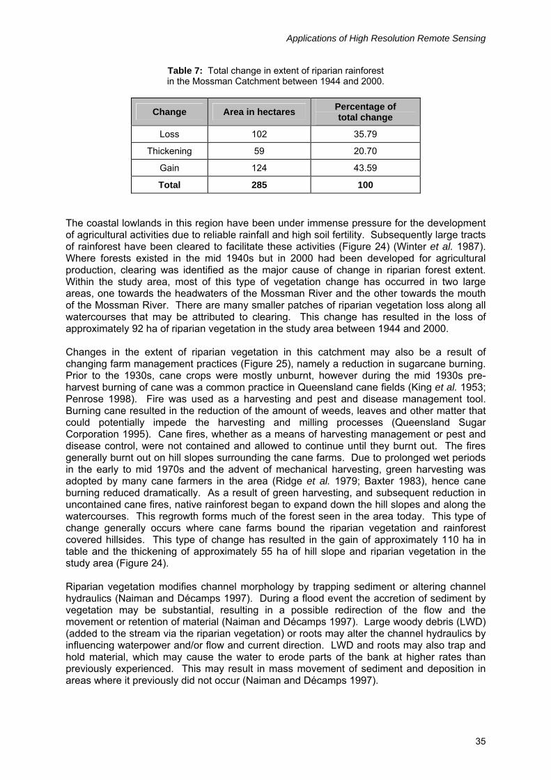
Figure 25: Example of riparian vegetation gain and thickening attributed to changes in farm management practices, South Mossman River .......................................37
Figure 26: Example of riparian vegetation change due to natural stream channel movement, South Mossman River and Cassowary Creek ..................................37


Applications of High Resolution Remote Sensing
1
1. INTRODUCTION Remote sensing science has provided new, synoptic views of ecological processes and land use impacts since the 1970s, and the development of digital image analysis in the late 1980s added a wide range of potential techniques for research applications. Remotely sensed data can be used to generate a wide range of estimates of forest structure and tree physiology that are of value to ecologists, including rainforest extent, canopy closure and connectivity, tree mortality, leaf area index (LAI), photosynthetic pigments and other indices of primary productivity. The increasing availability of high resolution satellite and airborne sensors (here defined as having an instantaneous field of view (IFOV) of less than 16 m2) has prompted new studies at local scales. These studies have permitted a better appreciation of the accuracy of modelled parameters and indices gained from low resolution sensors such as LANDSAT, AVHRR and MODIS (Roberts et al. 1998). In addition, they have allowed estimation of within-stand and individual tree canopy structure and physiology. The issue of scaling up from ground observations to satellite data is now more easily addressed, especially when local scale, plot measurements are complemented by spectral radiometry of individual plants, plots and stands. Implicit in all of these methodologies and their applications is the premise that there is a direct relationship between the forest structural and physiological parameters and the spectral reflectance as measured by the satellite or airborne sensor. Further, it is assumed that the spectral signatures of individual trees or forest types are unique and easily separable. A final assumption is that each pixel in the image is uniform, that is, contains only one vegetation type or cover class. If this last assumption is invalid, linear pixel un-mixing techniques (Adams et al. 1995) can resolve a limited number of components given adequate spectral resolution.

Applications of High Resolution Remote Sensing
3
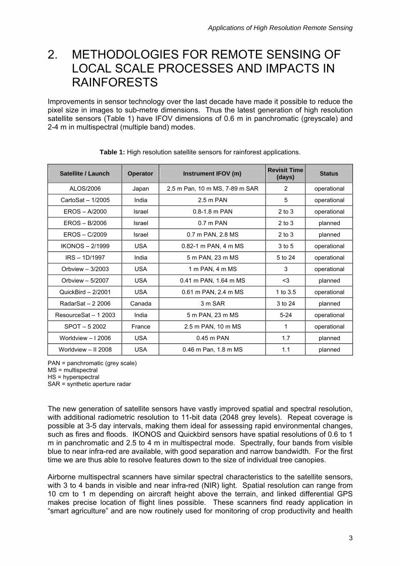
2. METHODOLOGIES FOR REMOTE SENSING OF LOCAL SCALE PROCESSES AND IMPACTS IN RAINFORESTS
Improvements in sensor technology over the last decade have made it possible to reduce the pixel size in images to sub-metre dimensions. Thus the latest generation of high resolution satellite sensors (Table 1) have IFOV dimensions of 0.6 m in panchromatic (greyscale) and 2-4 m in multispectral (multiple band) modes.
Table 1: High resolution satellite sensors for rainforest applications.
Satellite / Launch Operator Instrument IFOV (m) Revisit Time (days) Status
ALOS/2006 Japan 2.5 m Pan, 10 m MS, 7-89 m SAR 2 operational
CartoSat – 1/2005 India 2.5 m PAN 5 operational
EROS – A/2000 Israel 0.8-1.8 m PAN 2 to 3 operational
EROS – B/2006 Israel 0.7 m PAN 2 to 3 planned
EROS – C/2009 Israel 0.7 m PAN, 2.8 MS 2 to 3 planned
IKONOS – 2/1999 USA 0.82-1 m PAN, 4 m MS 3 to 5 operational
IRS – 1D/1997 India 5 m PAN, 23 m MS 5 to 24 operational
Orbview – 3/2003 USA 1 m PAN, 4 m MS 3 operational
Orbview – 5/2007 USA 0.41 m PAN, 1.64 m MS <3 planned
QuickBird – 2/2001 USA 0.61 m PAN, 2.4 m MS 1 to 3.5 operational
RadarSat – 2 2006 Canada 3 m SAR 3 to 24 planned
ResourceSat – 1 2003 India 5 m PAN, 23 m MS 5-24 operational
SPOT – 5 2002 France 2.5 m PAN, 10 m MS 1 operational
Worldview – I 2006 USA 0.45 m PAN 1.7 planned
Worldview – II 2008 USA 0.46 m Pan, 1.8 m MS 1.1 planned
PAN = panchromatic (grey scale) MS = multispectral HS = hyperspectral SAR = synthetic aperture radar The new generation of satellite sensors have vastly improved spatial and spectral resolution, with additional radiometric resolution to 11-bit data (2048 grey levels). Repeat coverage is possible at 3-5 day intervals, making them ideal for assessing rapid environmental changes, such as fires and floods. IKONOS and Quickbird sensors have spatial resolutions of 0.6 to 1 m in panchromatic and 2.5 to 4 m in multispectral mode. Spectrally, four bands from visible blue to near infra-red are available, with good separation and narrow bandwidth. For the first time we are thus able to resolve features down to the size of individual tree canopies. Airborne multispectral scanners have similar spectral characteristics to the satellite sensors, with 3 to 4 bands in visible and near infra-red (NIR) light. Spatial resolution can range from 10 cm to 1 m depending on aircraft height above the terrain, and linked differential GPS makes precise location of flight lines possible. These scanners find ready application in “smart agriculture” and are now routinely used for monitoring of crop productivity and health
Gillieson, Lawson and Searle
4
in many areas of intensive, irrigated agriculture worldwide. They have the advantage that recording of images over a given area can be virtually “on demand” given good weather and positioning of the aircraft and its sensor in the region. They are very useful for gaining high resolution images, similar to aerial photographs, to be used in forest extent mapping, or as backdrops in GIS analysis. Irrespective of whether a satellite or airborne high resolution sensor is used, there are some technical issues that have to be addressed if digital image analysis is contemplated. The first issue relates to the need to accurately orthorectify the image to a topographic map base, allowing integration with GIS and extraction of thematic features such as roads, buildings and forest margins. This requires a good network of accurately located ground control points (GCP) and a digital elevation model (DEM) with appropriate cell resolution. For many rainforest areas, we only have DEMs with cell resolutions of 30 to 80 m, which is insufficient precision for the task. Laser scanning techniques (LIDAR) and stereo models from aerial photography provide solutions to this problem, albeit at increased cost. The second issue relates to radiometric calibration, where the digital numbers (brightness values) in the image must be correlated with actual surface reflectance values. Most satellite sensors are well calibrated and maintain linearity throughout the full range of brightness values. For airborne scanners, this can be achieved using standard white and black reflectors placed in the field and recorded by the sensor at the same time as the rest of the scene. For some sensors, the relationship is non-linear at high reflectance values, limiting their utility. Finally, most of the airborne sensors use modified video cameras and lens curvature produces a vignetting effect, where image brightness decreases radially from the centre. This can be corrected given precise knowledge of the lens shape parameters and imaging geometry. High resolution imagery is typically used in a wide range of applications for image interpretation, cartography, and soft photogrammetry. Image interpretation can be either human, visual interpretation or automated, machine interpretation. Visual interpretation of orthorectified images is typically used in intelligence and disaster relief applications, and can also produce high quality results when used in combination with ancillary GIS data such as forest mensuration and detailed vegetation mapping. Machine interpretation is commonly used for land-use classification and feature extraction. Machine classification favors 11-bit products such as IKONOS that maintain absolute radiometric calibration of the multispectral imagery. There has been a recent move away from traditional, per-pixel classifiers towards object-oriented classifiers, which rely on a hierarchy of image segmentation producing polygons of similar spectral response, shape and area. Thus contextual concepts derived from landscape ecology and photo interpretation can now be integrated with image data. Derived image products such as vegetation indices can be used, with appropriate ground measurements, to develop robust relationships capable of predicting aboveground biomass and ultimately carbon accounting. Orthorectified images are the fundamental products for image maps, GIS image base, and cartographic extraction of infrastructure such as roads, buildings and drainage. GIS systems commonly show hydrographic, transportation, and other information as vector layers. Displaying those vectors on top of a base image adds useful context to the vector information.
Applications of High Resolution Remote Sensing
5
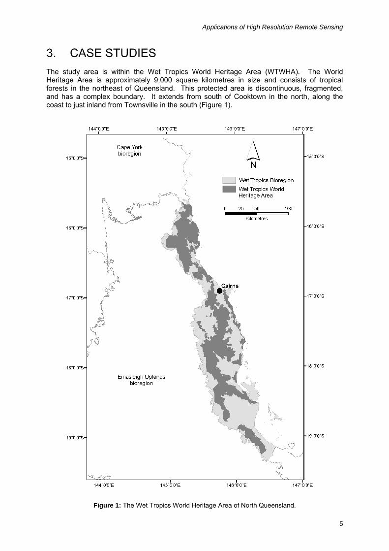
3. CASE STUDIES The study area is within the Wet Tropics World Heritage Area (WTWHA). The World Heritage Area is approximately 9,000 square kilometres in size and consists of tropical forests in the northeast of Queensland. This protected area is discontinuous, fragmented, and has a complex boundary. It extends from south of Cooktown in the north, along the coast to just inland from Townsville in the south (Figure 1).
Figure 1: The Wet Tropics World Heritage Area of North Queensland.

Gillieson, Lawson and Searle
6
In some places, the WTWHA begins at the edge of the Coral Sea in the east and spreads west across the coastal ranges. Immediately to the west of the coastal strip the steep forest-covered slopes again become part of the World Heritage Area. This extends westward over the Great Dividing Range and crosses undulating tablelands with gradually declining altitude and rainfall towards the west. The region is the most floristically rich area in Australia with over 3,500 species (Trott and Goosem 1996). This great diversity is related, in part, to the diversity in landform, where for instance the highest mountain in Northern Australia is 25 km from the sea. Deeply incised valleys and narrow ridges accentuate the dramatic relief. The area is also one of the wettest in Australia, with rainfall of about 2,000 mm recorded annually in many coastal towns and more than double this amount recorded in nearby mountains. Over half of the precipitation falls in the warmer months, December to March, but the orientation of the mountain ranges across the path of regular trade winds is conducive to orographic rainfall around the year. In this section we provide a number of examples using high resolution imagery to illustrate these various methods of digital image analysis. All are drawn from research carried out since year 2000 in the WTWHA under the auspices of the Cooperative Research Centre for Tropical Rainforest Ecology and Management (Rainforest CRC) in Cairns, North Queensland. 3.1 CANOPY DECLINE AND MORTALITY: MAPPING RAINFOREST
DIEBACK IN THE WET TROPICS
Dying and dead patches of rainforest associated with the root-rot fungus Phytophthora cinnamomi were first recorded in tropical North Queensland over twenty years ago (Brown 1976). Subsequent soil surveys showed the fungus was widespread and associated with serious disease in two widely separated rainforest areas in North Queensland, one of them in the WTWHA (Brown 1999). However little else is known of the threat posed by P. cinnamomi to the wet tropical rainforests of Queensland (Goosem and Tucker 1999). Worldwide, P. cinnamomi is regarded as one of the most destructive fungal pathogens of woody plants. In Australia, P. cinnamomi and other related species are responsible for economic losses totalling millions of dollars annually, and dieback caused by P. cinnamomi is listed as a key threatening process under the federal Endangered Species Protection of Biodiversity Act (1999). As a consequence, systematic identification and mapping of areas currently affected by dieback and those that are potentially susceptible to it have been given very high priority by the Wet Topics Management Agency (WTMA) based in Cairns. During the earlier soil surveys undertaken by Brown and colleagues (Brown 1999), P. cinnamomi was detected in 645 of the 1,817 sites sampled. Its occurrence was not always associated with dieback but detection rates were significantly higher under patches of dead and dying forest. Interpretation of aerial photography in the Eungella Tableland near Mackay showed that dieback patches occupied some 19% (125 ha) of the study area. The specific objectives of this project in year 2000 were to: • Mark-up and interpret observable canopy dieback on aerial photography and satellite
imagery;
• Determine the environmental correlates of canopy dieback patches in three study areas; and

Applications of High Resolution Remote Sensing
7
• Develop an index of canopy dieback patches for application to remotely sensed data at a variety of spatial scales.
These objectives provide a strategy for enhanced understanding of the spatial extent of canopy dieback and its relationship to environmental variables such as topography, geology and vegetation. In addition, relationships with other variables such as the distribution of roads and drainage can be sought. The patches provide an unbiased sampling frame with which to determine the precise spatial signature of canopy dieback. This will be of great assistance in extending the regional survey across the entire WTWHA. It will also provide a means of scaling up from high-resolution multispectral imagery (at 2 m resolution) to commercially available Landsat ETM data with 25 m resolution. Three study areas were selected on the basis of historical evidence (Brown 1976, 1999) of rainforest canopy dieback: Tully Falls-Koombooloomba; Lamb Range and Mount Lewis. Over 250 canopy dieback patches were mapped and thus provide a reasonable sample from which to infer environmental correlates. The precise locations of dieback patches were mapped from colour aerial photography at a scale of 1:25,000. Areas of reduced canopy density or canopy senescence (brown) were delineated as polygons on transparent overlays and transferred to topographic maps at a scale of 1:50,000. These polygons were then digitised and stored as AutoCad (.dxf) files, attributed and converted to shapefiles (.shp) in ArcView 3.2 GIS software. In addition, remotely sensed data were acquired – Landsat ETM+ multispectral imagery for September 1999 was sourced from ACRES and precision map oriented (to level 9). This imagery comprises seven spectral bands from visible blue to near thermal infra-red, with an additional panchromatic layer in the visible blue to red area of the spectrum. Spatial resolution is 25 m and RMS error on rectification is 12 m. These data cover the entire WTWHA and potentially provide a valuable resource for dieback mapping and derivation of other spatial data layers in a GIS. Airborne multispectral videography was sourced from the Farrer Centre, Charles Sturt University. Four calibrated and filtered video cameras with 12 mm focal length lens on each camera give 2 m by 2 m pixels at 2,800 m altitude. Each camera gives an image of 740 by 576 pixels, resulting in ground coverage of 1,500 by 1,100 m or approximately 165 ha. This is coupled with differential GPS, which gives the location of the centre of each image. The four spectral bands in these data are directly comparable with the Landsat ETM+ imagery, allowing for potential scaling up of spectral signatures. A detailed GIS analysis of the spatial association between dieback patches and environmental variables was carried out (Gillieson et al. 2002). Most dieback patches occur in simple notophyll vine forest (Webb and Tracey types 8/9). Small numbers of patches also occur in complex notophyll vine forest (type 5a), several mesophyll forest types (types 1a, 1b, 2a), and closed forest with eucalypts (type 13c). The distribution of patch areas by vegetation type (Figure 2) indicates that there is a strong spatial correlation between dieback patches and notophyll forest types (Table 2).
Gillieson, Lawson and Searle
8
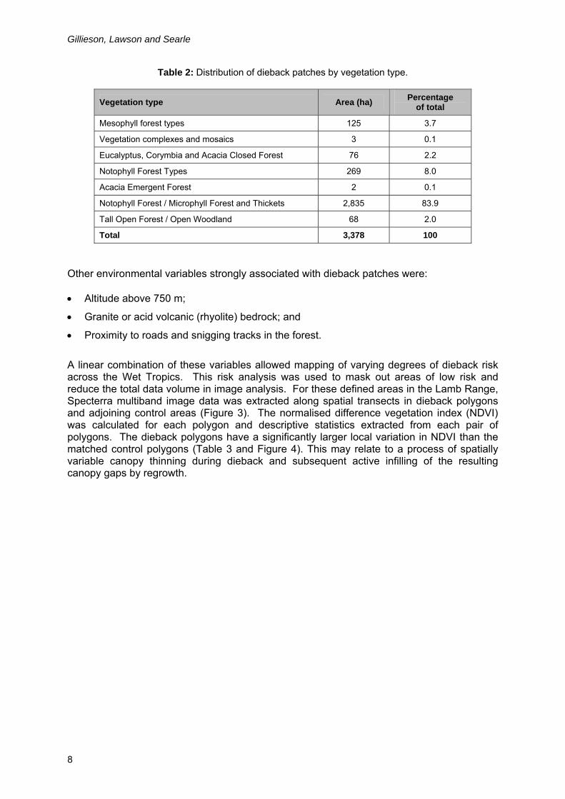
Table 2: Distribution of dieback patches by vegetation type.
Vegetation type Area (ha) Percentage of total
Mesophyll forest types 125 3.7
Vegetation complexes and mosaics 3 0.1
Eucalyptus, Corymbia and Acacia Closed Forest 76 2.2
Notophyll Forest Types 269 8.0
Acacia Emergent Forest 2 0.1
Notophyll Forest / Microphyll Forest and Thickets 2,835 83.9
Tall Open Forest / Open Woodland 68 2.0
Total 3,378 100
Other environmental variables strongly associated with dieback patches were: • Altitude above 750 m;
• Granite or acid volcanic (rhyolite) bedrock; and
• Proximity to roads and snigging tracks in the forest.
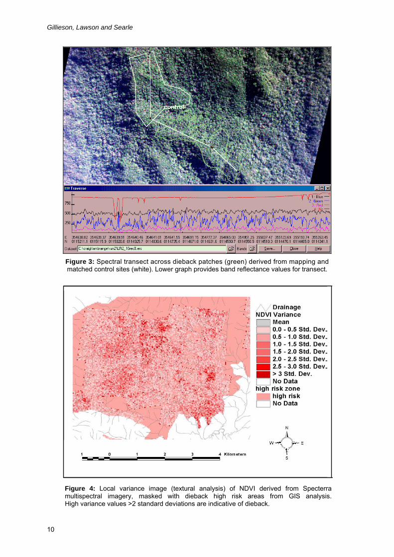
A linear combination of these variables allowed mapping of varying degrees of dieback risk across the Wet Tropics. This risk analysis was used to mask out areas of low risk and reduce the total data volume in image analysis. For these defined areas in the Lamb Range, Specterra multiband image data was extracted along spatial transects in dieback polygons and adjoining control areas (Figure 3). The normalised difference vegetation index (NDVI) was calculated for each polygon and descriptive statistics extracted from each pair of polygons. The dieback polygons have a significantly larger local variation in NDVI than the matched control polygons (Table 3 and Figure 4). This may relate to a process of spatially variable canopy thinning during dieback and subsequent active infilling of the resulting canopy gaps by regrowth.

Applications of High Resolution Remote Sensing
9
Figure 2: Distribution of recorded dieback patches overlain on vegetation (structural types) of the Tully Falls area. Note the strong spatial association between dieback occurrence and notophyll forest types (Webb and Tracey types 8/9).
Vegetation Types and Dieback Areas near Tully Falls
Gillieson, Lawson and Searle
10
Figure 3: Spectral transect across dieback patches (green) derived from mapping and matched control sites (white). Lower graph provides band reflectance values for transect.
Figure 4: Local variance image (textural analysis) of NDVI derived from Specterra multispectral imagery, masked with dieback high risk areas from GIS analysis. High variance values >2 standard deviations are indicative of dieback.

Applications of High Resolution Remote Sensing
11
Table 3: Derived statistics from analysis of Lamb Range dieback polygons and matched control sites.
Variable Dieback Control F ratio
Mean NDVI 0.7959 0.7958 0.00
Sigma NDVI 0.051 0.044 6.88***
Coeff. Variation NDVI 6.45 5.62 5.69***
*** significant at 0.01 level, n=66 The dieback patches are relatively small (usually less than five tree canopies) and may not be detected by Landsat imagery with a resolution of 30 m. It is better to use high resolution multispectral data (1 to 2 m resolution) such as Specterra. In general, average canopy NDVI is not a good indicator of canopy decline in these rainforests, but local variance of NDVI is a more useful index. This evaluation allows more focused field investigations in areas of both high canopy variance and high risk from the GIS analysis. 3.2 MAPPING THE EXTENT OF WEEDS IN THE WET TROPICS
It is well accepted that rates of forest destruction and fragmentation around the globe have been higher in the last century than at any other time. In the wet tropical zone of Queensland, the World Heritage Convention has protected much of the publicly owned tropical rainforest from logging and clearing, but other more insidious threats remain. In efforts to conserve and present the values of the WTWHA, the Wet Tropics Management Authority (WTMA) focuses research and management strategies to reduce or remove threats to the natural and cultural values of the area. Several linear corridors providing road and electricity services fragment the WTWHA. Fragmentation and invasive pest species are priority areas of research effort in the WTWHA. Weeds contribute to fragmentation effects by competition with native species and inducing disturbances such as fire. There is a need to develop less field-intensive methods of detection of invasions of new weed species, and prediction of expansion of existing weed problems (WTMA, 1999). Remote sensing has the potential to provide a practical and cost-effective way of monitoring threats such as weed incursion especially where seasonally wet roads prevent access. Remote sensing has frequently been used for monitoring broad-scale land clearing but not so for local changes involving subtle changes in spectral reflectance of vegetation. It can give timely, up-to-date information on the distribution and abundance of weeds over a wide area, especially where seasonally wet roads prevent continuous access to some locations. It can discern small patches at a local scale of square metres as well as surveying over broad scales of square kilometres. However, limited use and development of remote sensing in rainforest environments has occurred in Australia (Phinn et al. 2000). There is some difficulty in relating one remotely sensed image to another taken at a different time, so multitemporal analysis of imagery has been restricted mostly to spatial changes rather than spectral changes (Adams et al. 1995). Thus, remote sensing is used for monitoring land clearing but not for subtle changes in forest type. By quantitatively relating imagery to ground measurements, this study will elucidate the main difficulties and suggest a way forward in examination of subtle differences in the reflectance of vegetation types such as weeds. The ability of a Geographic Information System (GIS) to integrate remote sensing data also allows development of predictive modelling that could provide a powerful tool in monitoring

Gillieson, Lawson and Searle
12
the spread of an aggressive weed such as Pond apple (Annona glabra), and assisting management to design control strategies. This study examines the general criteria needed for quantitative ground measurements of reflectance to be used in classifying the spectral differences of weed species. The specific focus being the determination of the fractional quantity of each weed species at the sub-pixel level using Spectral Mixture Analysis (SMA), and what spatial, spectral and radiometric resolution is required. Despite being fragmented in the past by extensive and patchy land clearing for agriculture, several linear corridors providing road and electricity services traverse some of the larger sections of the World Heritage Area. A powerline corridor near Lake Morris was examined in detail at seven locations. The focus of this study is on these seven sites, surrounding towers in the Chalumbin-Woree powerline corridor. The corridor passes through World Heritage listed forest, from Bridle Creek (near Davies Creek), to Woree, a suburb of Cairns. Figure 5 shows a colour composite satellite image of the study area. The Bridle Creek section consists of low to medium woodland (type 16c, h, i, m) and the corridor passes through closed forest (with Eucalyptus, Corymbia and Acacia emergents – type 13c) with the remainder (the major portion of the corridor) passing through mesophyll vine forest (type 2a, Tracey and Webb, 1975).
Lake Morris
Davies Ck
Bridle Ck
Shoteel Ck Crystal CascadesFreshwater Ck
Cairns 9km
CopperlodeDam
0 1 2 3 Kilometers Study sites N
Powerline Corridor
Powerline Corridor
Figure 5: IKONOS satellite image of the study area showing the powerline towers within the study sites as red dots.
Percentage cover was measured by a stratified sampling method to obtain an estimation of the composition of vegetation leaf area in relatively pure plots at each site, with the aim of being able to assess the accuracy of the species identity in the image classification (ground truthing). The sites were divided into two or three relatively homogeneous areas that were thought to be large enough to be visible from the air. In each area, three to four quadrats of each square metre were examined visually for species content. Assessment was based on the percentage of leaf area. Each square-metre quadrat had twenty-five cells marked within it to facilitate the estimation. Percentage leaf area in each cell was estimated and the results

Applications of High Resolution Remote Sensing
13
pooled for each quadrat. A vertical photograph was taken and a reading was made with the Cropscan spectral radiometer and a Global Positioning System (Garmin 12XL GPS). All plants at each site were identified by a professional botanist (Mr Robert Jago). Samples of the spectral reflective response of particular weed species were collected from powerline corridors throughout the WTWHA with a Cropscan MSR. Specific areas visited were: Tully Gorge to Palmerston in the south east, Chalumbin to Tully Gorge, Mt Evelyn, Chalumbin to Woree, Black Mountain Road and Rex Range, Mount Lewis, and the CREB Track in the north. The direct output in millivolts was recorded on a data logger along with time, date, sun angle, and irradiance in W/m2. When the data was downloaded the millivolt readings for each band in the up and down direction were converted to percentage reflectance using the calibration constants in the file header. Four readings were taken in the same vicinity for each species sample. The data was downloaded and post-processed into percentage reflectance. Imagery of the powerline corridor was acquired at two different spatial scales (Figure 6). One source was IKONOS multispectral satellite at 4 m resolution, and the other was an Airborne Data Acquisition and Registration (ADAR) camera system at approximately 1 m ground resolution.
IKONOSSatellite Imagery
ADAR Imagery
Field spectralresponse data
analysis
Classify withfield data
Classify withfield data
Classify
Classify
Calibrate
CalibrateField spectralresponse data
analysis
Figure 6: Integrated research methodology used for weed assessment and scaling up from field observations to satellite image data.
There were 41 weed species, and within each square metre, one to three of these species were present, suggesting that Spectral Mixture Analysis was possible in imagery at 1 m spatial resolution.

Gillieson, Lawson and Searle
14
Spectral reflectance measurements of weed species showed that the variability within some species was much higher than the apparent differences between species (Figure 7). This is especially true of the varied colour forms of Lantana camara. The numerical resolution was high enough to separate species, however the spectral classes found were further subdivided to a species level and entered into a statistics program (SPSS) for discriminant analysis. This found that many mono-specific classes of reflectance were actually statistically discernible. Figure 8 is a “supervised” classification where known class signatures are assigned to each pixel based on the closeness of the signature mean to the value of each pixel (dn in each band). The choice of classifiers is open to the user and the essential requirements of it being that it is reliable in performance.
0
10
20
30
40
50
60
70
460 510 560 610 660 710 760 810
wavelength (nm)
% re
flect
ance
blady grass
blady grass
Blady grass ch
Blady grass ch
Blady grass ch
Blady grass ch
Blady grass ch
Blady grass ch
Blady grass ch
Blady grass ch
Blady grass ch
Blady grass ch
blue snakeweed -- somedark blue flowersblue snakeweed -- somedark blue flowersblue snakeweed -- somedark blue flowersblue snakeweed -- somedark blue flowersblue snakeweed 60% /molasses grassblue snakeweed 60% /molasses grassblue snakeweed 60% /molasses grassblue snakeweed 60% /molasses grass
Figure 7: Reflective differences within and between blady grass and blue snakeweed. An empirical calibration was employed to relate field spectral responses to the imagery, avoiding complex atmospheric corrections. However difficulty was experienced with calibration of the ADAR imagery due to an inherent interpolation algorithm in the camera's electronics. While adequate for production of natural colour digital images, it precludes use of the data for quantitative analysis. The Spectral Mixture Analysis (SMA) was found to be unsuitable as a classifier of the ADAR imagery possibly because of poor camera performance. Figure 9 shows the fraction of a signature that is itself a mixture (containing mostly Rubus). It was also unsuitable for the spatial resolution of the IKONOS imagery being only four bands to unmix the contents of a 4 m x 4 m ground resolution element. Vegetation response patterns are broad and highly reflective in the near infra-red wavelengths contributing to non-linear mixing of the spectral components. Thus the Linear Unmixing algorithm (below) of this classifier was found to be unsuitable for discrimination of fine spectral classes that have a large variation in their signature from site to site.

Applications of High Resolution Remote Sensing
15
Pixel reflectancein 3 bands of imagery
+ error
+ error residual
+ error
r1 = ajxj + akxk + alxl
r2 = bjxj + bkxk + blxl
r3 = cjxj + ckxk + clxl
3 end-members (weed spp j, k, l) each with reflectance in 3 bands (a, b, c)
Figure 8: Minimum distance classification (broad groups) developed from training sites
in an image from the Bridle Creek section of the Chalumbin-Woree powerline.
Figure 9: Proportion of spectral group 14, which is a mixture of
mostly Rubus, Dicranopteris, Alpinia spp. and Panicum.

Gillieson, Lawson and Searle
16
We concluded that detailed quantitative analysis of ADAR imagery is unproductive and that the 4 m spatial resolution of the IKONOS Satellite imagery is too coarse to adequately discern different weed species in this rainforested area. We recommended that further work be done to better characterise the variety of spectral signatures of weeds and that quantitative analysis use multispectral sensors at a ground resolution of less than 2 m. Spectral reflectance measurements taken of standard targets at the time of flying would enable better calibration, which is important for relating field measurements to the imagery. Future work also requires software with signature portability and an ability to take advantage of the high dynamic range of modem sensors. Classification at the sub-pixel level needs to adequately allow for the variability of vegetation spectral response by the use of appropriate statistics, for example “Fuzzy Set” theory. 3.3 ASSESSING CANOPY CONNECTIVITY ACROSS ROADS IN
RAINFOREST AREAS
Road ecology is a rapidly developing branch of landscape ecology, which focuses attention on the roles of roads as barriers to wildlife movement and as agents of fragmentation in forested landscapes (Forman and Alexander 1998). Few studies have been carried out on the ecology of roads in the humid tropics (Laurance et al. 2004; Goosem 2000), but there is a rapidly growing literature on the ecological effects of roads in temperate landscapes (Forman et al. 2003). Roads affect wildlife in several ways at a variety of spatial scales. At a local scale, individual stretches of road with traffic form behavioural barriers to the movement of wildlife; there may be mortality due to animals being run over, or the combination of road verge and pavement may inhibit or preclude animals from attempting to cross the road. The condition of the road verge may influence the risk: densely forested or shrub covered verges may be conducive to movement, but the rapid emergence of animals onto the road pavement may increase mortality at “black spots” (Goosem 2002). Culverts may provide a safer alternative, and innovative research (Goosem 2003) into culvert design and “furniture” may enhance their value for wildlife. For arboreal mammals, canopy connectivity is critical. Tree canopies must interfinger over a sufficient distance to allow free animal movement, though research on canopy bridges provides a viable alternative. At a landscape scale, roads drastically reduce landscape connectivity between suitable habitat patches, creating isolated metapopulations that then become vulnerable to predation, disease and loss of genetic diversity (Spellerberg 1998). Competition for territory may displace individuals to the margins of forest patches, where they occupy marginal habitats and become more vulnerable. At a regional scale, fragmentation due to roads can result in reduced regional populations of species and inhibit their persistence in the smallest patches of forest. In this study we estimated the forest canopy coverage and connectivity across a major road that runs through the WTWHA. The Kuranda Range Road (Figure 10) is the major arterial link between Cairns and nearby towns (Kuranda, Mareeba, Atherton) on the northern Atherton Tableland. It carries high volumes of traffic comprised of commuting residents, trucks and tourists. The road passes through tropical rainforest communities as well as cleared land, regrowth and residential areas. The production of a detailed coverage of the road corridor was achieved by the integration of spatial data in different formats in ArcGIS 8.3. The imagery used was pan-sharpened IKONOS multispectral data, orthorectified using OrthoWarp 2.3 to achieve a root mean

Applications of High Resolution Remote Sensing
17
square error of <10 cm in plan. This provided four bands (blue, green, red, near infra-red) with a resolution of 1 m. A vector coverage in AutoCAD format provided road centreline and pavement edge data, based on ground surveys carried out by the Queensland Department of Main Roads; this has millimetric precision. The IKONOS imagery was classified using an ISODATA unsupervised classification in ER-Mapper 6.4 to identify spectral classes of information. There was very good separability between forest canopy and road pavement due to the greater data range in IKONOS (11-bit). In addition, spectral properties of individual image bands were used to differentiate between road and woody vegetation; a series of spectral transects across the road used NIR/Red thresholding (Figure 11) to confirm separability. The binary image was then converted to vector.
Figure 10: Kuranda Range road overlain on visualisation of terrain and rainforest vegetation.

Gillieson, Lawson and Searle
18
Figure 11: Spectral transect across Kuranda Range road at 9 km from start, showing decline in NIR reflectance across road base. Vertical lines indicate surveyed edge of road base.
The vector road data was cleaned and extraneous linework removed, leaving pavement edges and centerline. Missing sections of centerline were reconstructed using an intersection of arcs pivoted on the pavement edge. The road pavement vectors were then intersected with the classified image to yield a linear vector dataset, which was bounded by the road edge and contained two categories, road and forest. This vector dataset was subdivided into individual numbered polygons (forest canopy and road) and used in all subsequent spatial analysis, overlain on the IKONOS image (Figure 12) to allow checking of accuracy.
Figure 12: Canopy overhang polygons overlain on visualisation of terrain and rainforest canopy image (IKONOS infrared false colour composite).

Applications of High Resolution Remote Sensing
19
Canopy coverage was calculated as the percentage area of forest canopy in each 100 m segment of the road (total length 13 km). Canopy connectivity was defined by identifying all groups of contiguous polygons, which intersected both pavement edges. A total of fifty-five connections were identified. The area (in square metres) and perimeter (in metres) of each connected polygon cluster was then calculated. Areas of individual polygons ranged from 2 to 823 m2 with a mean of 211 m2. The distribution of connected polygons reveals a large number of small area connections and a few large area connections (Figure 13). A shape index was derived using a vector interpolation method (triangulated irregular network or TIN). Each polygon cluster was subdivided into the minimum number of triangles that infilled the space. Two statistics were calculated. • Average Area of the triangles in a polygon = Polygon area / Number of triangles; and
• Shape Index = Polygon perimeter / Average area of triangle.
These two statistics permitted an evaluation of the quality of each canopy connection across the Kuranda Range Road.
Figure 13: Distribution of connected canopy polygons along 19 km of the Kuranda Range road.
Gillieson, Lawson and Searle
20
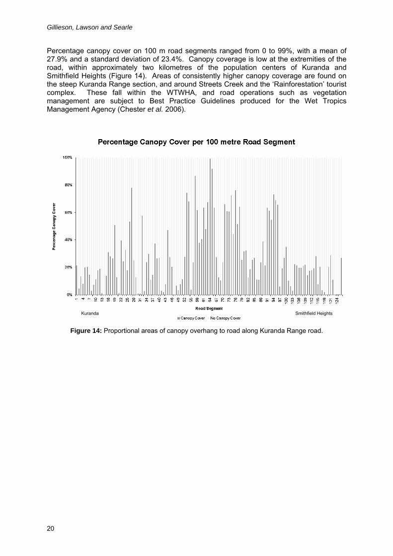
Percentage canopy cover on 100 m road segments ranged from 0 to 99%, with a mean of 27.9% and a standard deviation of 23.4%. Canopy coverage is low at the extremities of the road, within approximately two kilometres of the population centers of Kuranda and Smithfield Heights (Figure 14). Areas of consistently higher canopy coverage are found on the steep Kuranda Range section, and around Streets Creek and the ‘Rainforestation’ tourist complex. These fall within the WTWHA, and road operations such as vegetation management are subject to Best Practice Guidelines produced for the Wet Tropics Management Agency (Chester et al. 2006).
Kuranda Smithfield Heights
Figure 14: Proportional areas of canopy overhang to road along Kuranda Range road.

Applications of High Resolution Remote Sensing
21
Figure 15: Analysis of individual canopy overhang polygons providing shape statistics.
The degree and quality of canopy connectivity across the road can be assessed using the derived statistics (Figure 15). Connectivity has to be assessed in terms of the area of the canopy connection and the shape index; high area and low shape index indicate a connection that presents many points of contact and tends to a rectangular shape, rather than connections that are tangential and consist of linear strips along each side of the road. There are a number of connections that have moderate area (500 to 1,000 m2) and low shape index (15 to 20) (Figure 16), which may provide opportunities for marsupials and birds to move across the road corridor. Connections with an area of less than 200 m2, though having a low shape index, may only provide one point for crossing and are thus vulnerable to disturbance. Many semi-trailers use the road and their roofs may come within a few metres of the forest vegetation. Areas with high quality canopy connectivity may need to be flagged to avoid disturbance and disruption.

Gillieson, Lawson and Searle
22
Figure 16: Canopy connectivity measures based on analysis of canopy overhang polygons.
The accuracy of the canopy connectivity estimates was evaluated by walking the road and visiting each indicated connection, using a GPS receiver to locate it. Indicated connections were rated into one of four categories as follows: • Unconnected – overlapping but vertically separated by more than 50 cm, or horizontally
by a gap of more than one metre;
• Poor – canopies overlapping but touching at one point only, over a distance of less than five metres, little interfingering of branches;
• Good – canopies overlapping over a distance of at least five metres, good interfingering of branches;
• Very Good – canopies over lapping over a distance of more than ten metres, good interfingering of branches, numerous connection points obvious.

Applications of High Resolution Remote Sensing
23
Table 4: Field evaluation of canopy connectivity, Kuranda Range Road.
Quality Number Percentage
Unconnected 33 49.25
Poor 19 28.36
Good 11 16.42
Very good 4 5.97
Additional canopy connections not indicated in the spatial analysis were noted and their position determined. Only two such canopy connections were located. Where variation was noted in the connection quality, additional connections were noted for that polygon. Fifty one percent of estimated canopy connections were found to be actually connected, but of these four were very good, eleven good and nineteen poor (Table 4). Of the estimated connections that were in fact unconnected, about half (n=16) were the result of tree canopies overlapping in plan but not in elevation; there was thus a vertical separation of one and five metres between the tree canopies. It is not possible to distinguish these in the spatial analysis, as the IKONOS imagery only provides a vertical view of the canopy. This study has provided an integrative methodology for assessing canopy cover and connectivity across road and other corridors in tropical rainforests. Its main advantage is that it provides a rapid and objective means of measuring connectivity, and of targeting subsequent fieldwork to evaluate the quality of individual connections. Other applications could be found in assessing the quality and quantity of revegetation patches across powerline corridors, or, given suitable stream channel definition, connectivity across tropical streams.
Gillieson, Lawson and Searle
24
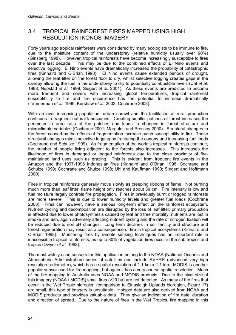
3.4 TROPICAL RAINFOREST FIRES MAPPED USING HIGH RESOLUTION IKONOS IMAGERY
Forty years ago tropical rainforests were considered by many ecologists to be immune to fire, due to the moisture content of the understorey (relative humidity usually over 90%) (Ginsberg 1998). However, tropical rainforests have become increasingly susceptible to fires over the last decade. This may be due to the combined effects of El Nino events and selective logging. El Nino events have dramatically increased the probability of catastrophic fires (Kinnaird and O’Brian 1998). El Nino events cause extended periods of drought, allowing the leaf litter on the forest floor to dry, whilst selective logging creates gaps in the canopy allowing the fuel in the understorey to dry to potentially combustible levels (Uhl et al. 1988; Nepstad et al. 1999; Siegert et al. 2001). As these events are predicted to become more frequent and severe with increasing global temperatures, tropical rainforest susceptibility to fire and fire occurrence has the potential to increase dramatically (Timmerman et al. 1999; Kershaw et al. 2003; Cochrane 2003). With an ever increasing population, urban sprawl and the facilitation of rural production continues to fragment natural landscapes. Creating smaller patches of forest increases the perimeter to area ratio of the patches and leads to changes in forest structure and microclimate variables (Cochrane 2001; Margules and Pressey 2000). Structural changes to the forest caused by the effects of fragmentation increase patch susceptibility to fire. These structural changes mimic selective logging by fracturing the canopy and increasing fuel loads (Cochrane and Schulze 1999). As fragmentation of the world’s tropical rainforests continue, the number of people living adjacent to the forests also increases. This increases the likelihood of fires in damaged or logged rainforests due to the close proximity of fire-maintained land uses such as grazing. This is evident from frequent fire events in the Amazon and the 1997-1998 Indonesian fires (Kinnaird and O’Brian 1998; Cochrane and Schulze 1999; Cochrane and Shulze 1998; Uhl and Kauffman 1990; Siegert and Hoffmann 2000). Fires in tropical rainforests generally move slowly as creeping ribbons of flame. Not burning much more than leaf litter, flame height only reaches about 30 cm. Fire intensity is low and fuel moisture largely controls fire propagation. Fires in previously burnt or logged rainforests are more severe. This is due to lower humidity levels and greater fuel loads (Cochrane 2003). Fires can however, have a serious long-term effect on the rainforest ecosystem. Nutrient cycling and decomposition are disrupted by the loss of leaf litter; primary production is affected due to lower photosynthesis caused by leaf and tree mortality; nutrients are lost in smoke and ash, again adversely affecting nutrient cycling and the rate of nitrogen fixation will be reduced due to soil pH changes. Long term declines in soil fertility and structure and forest regeneration may result as a consequence of fire in tropical ecosystems (Kinnaird and O’Brian 1998). Monitoring fires by remote sensing techniques has an important role in inaccessible tropical rainforests, as up to 80% of vegetation fires occur in the sub tropics and tropics (Dwyer et al. 1998). The most widely used sensors for this application belong to the NOAA (National Oceanic and Atmospheric Administration) series of satellites and include AVHRR (advanced very high resolution radiometer), which has a spatial resolution of 1.1 km x 1.1 km. MODIS is another popular sensor used for fire mapping, but again it has a very course spatial resolution. Much of the fire mapping in Australia uses NOAA and MODIS products. Due to the pixel size of this imagery (NOAA / MODIS) small fires (>20 ha) are not detected. As many of the fires that occur in the Wet Tropic bioregion (comparison to Einasleigh Uplands bioregion, Figure 17) are small, this type of imagery is unsuitable. Hotspot data are also derived from NOAA and MODIS products and provides valuable data. They give an indication of fire date, duration and direction of spread. Due to the nature of fires in the Wet Tropics, fire mapping in this

Applications of High Resolution Remote Sensing
25
area needs to be much finer detail than that achievable from NOAA or MODIS data as fires are patchy and generally under 20 ha, thus imagery with a finer resolution is required.
Figure 17: Monthly distribution of bushfire scars by area (in hectares) for the Wet Tropics (WET) and Einasleigh Uplands (EIU) bioregions of Queensland.
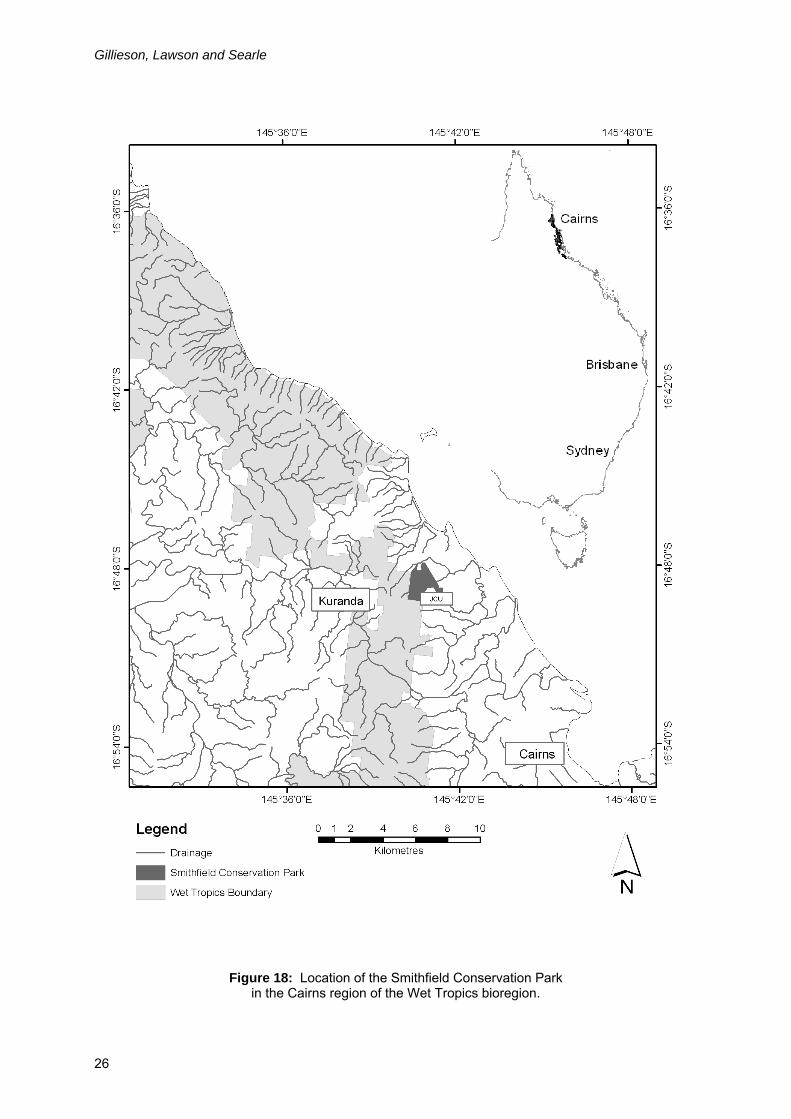
Data supplied by Cape York Peninsula Development Association. With the launch of the IKONOS satellite in September 1999, a new era of satellite imagery with resolution comparable to aerial photographs has become available (Dial and Grodecki 2003; Goetz et al. 2003). IKONOS provides 4 m multispectral and 1 m panchromatic image data (Dial and Grodecki 2003). This imagery has many applications including the assessment of natural disasters such as wildfire and cyclones, and monitoring and management of wetlands, parks and protected lands (Goetz et al. 2003). IKONOS imagery has been previously used to: differentiate between forest stand age classes (Kayitakire et al. 2002); estimate tree crown diameter (Asner et al. 2002); detecting mountain pine beetle infestation (White et al. 2005); quantifying tropical rainforest tree mortality (Clark et al. 2004); and to map forest degradation (Souza Jr. and Roberts 2005). This study reports on the use of multitemporal IKONOS imagery for fire scar mapping in a tropical rainforest in North Queensland, Australia. This study was undertaken in the Smithfield Conservation Park (SCP), 17 km north of Cairns (16°48’S, 14°541’E) (Figure 18) in the Wet Tropics bioregion of northern Queensland, Australia. The climate in this area is characterised by relatively dry mild winters and hot humid summers with rainfall averaging 2,100 mm per annum (Marrinan et al. 2005). The Smithfield Conservation Park covers an area of approximately 270 ha, of which about 180 ha is rainforest vegetation. The rough terrain supports rainforest vegetation types such as mesophyll vine forest, complex notophyll vine forest and simple notophyll vine forest (Stanton and Stanton 2003).
Gillieson, Lawson and Searle
26
Figure 18: Location of the Smithfield Conservation Park
in the Cairns region of the Wet Tropics bioregion.

Applications of High Resolution Remote Sensing
27
Extreme El Nino events are common in Queensland. Table 5 highlights drought duration and rainfall for Kuranda railway station from 1898 to 2005, while Figure 19 shows the occurrence of moderate and severe droughts in the Cairns region. The most severe drought was experienced in 2001-2002, which resulted in only 721 mm annual rainfall in the Cairns region – the lowest annual rainfall ever recorded for the region. This is well below the annual average of 2,100 mm. This extended dry period (23 months in total) had serious consequences for the WTWHA.
Table 5: Drought duration and rainfall data for Kuranda railway station from 1898 to 2005.
Period Duration (months) Driest 12 months Average SOI
May 2001 to Mar 2003 23 831 -4.8
Mar 1991 to Nov 1992 21 877 -11
Feb 1989 to Jan 1990 12 1,015 5.6
Mar 1981 to Feb 1982 12 1,029 2.7
Oct 1965 to Jan 1967 16 864 -4
Mar 1960 to Dec 1961 22 847 2.6
Jan 1951 to Dec 1951 12 1,036 -0.7
Feb 1946 to Mar 1947 14 1,016 -5.4
Jul 1925 to Aug 1926 14 1,037 -8.5
Figure 19: Occurrence of moderate and severe droughts in the Cairns region. Data from Kuranda Railway Station, processed in Rainman-Streamflow software.

Gillieson, Lawson and Searle
28
The fire that swept through the Smithfield Conservation Park in November 2002 burnt approximately 150 ha of the 180 ha of rainforest vegetation (Marrinan et al. 2005). This was a one in one hundred year event, which patchily burnt the steep rainforested ridges of the McAllister Range over a three-week period. An extremely dry period in 2002 led to a large amount of dry leaf litter on the forest floor and this fuelled the fire (Marrinan et al. 2005). The fire burnt significant remaining examples of lowland Complex Mesophyll Vine Forest and Mesophyll Vine Forest. Fire intensity for this event was thought to be low, as canopy scorching was absent and the distribution of fire scars at the bases of trees suggests that flame height was also only low (Marrinan et al. 2005). The IKONOS images of Smithfield (Table 6) were orthorectified using the OrthoWarp 2.3 extension for ER-Mapper 6.4. The process used the 10 m DEM derived from the 1:25,000 digital topographic data published by the Queensland Department of Natural Resources, Mines and Water. The DEM was produced by Searle Consulting NQ, using the minimum curvature algorithm in the gridding function of ER-Mapper. Ground control points were established to centimetre accuracy using GPS survey techniques. The IKONOS imagery is comprised of five bands and provides 4 m spatial resolution multispectral (red (1), green (2), blue (3) and near infrared (4) bands) and 1 m spatial resolution panchromatic (band 5) imagery (Aplin 2003). The entire image processing for this study was undertaken using ER-Mapper 6.4 and Idrisi 3.2.
Table 6: Details of satellite imagery used in this analysis.
Source Images 2002 2004
Sensor IKONOS-2 IKONOS-2
Date 29/01/2002 17/06/2004
Solar azimuth angle 95.9030 31.6533
Solar zenith angle 25.4743 46.7594
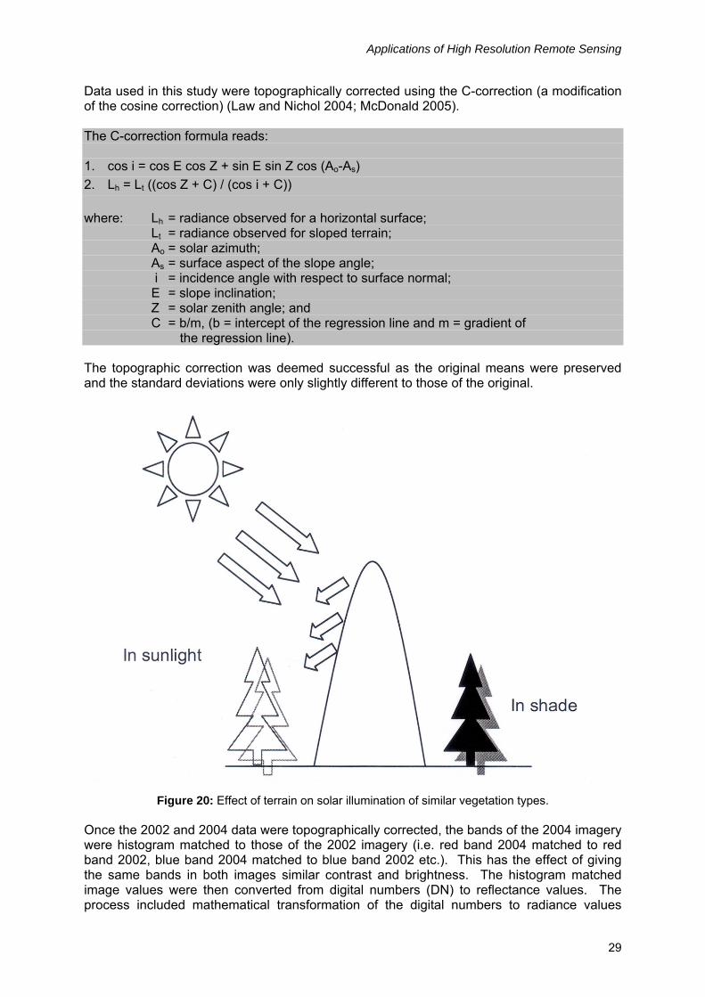
Topographic correction of this imagery was necessary as in this area of rugged terrain similar vegetation types may vary highly in their spectral response due to the shape of the terrain and low solar illumination angle, creating a shadowing effect (Figure 20; McDonald 2005; Raino et al. 2003). Areas in high solar illumination may show higher than expected reflectance while areas in shade may show lower than expected reflectance. Hence topographic correction will even out the reflectance of areas in solar illumination with those in shade. The most commonly used topographic correction is the cosine correction. The cosine correction however was found by Law and Nichol (2004) to be unsuitable for IKONOS imagery due to overcorrection. The cosine correction was also found to overcorrect in areas of rough terrain (Law and Nichol 2004) and thus is not suitable for areas such as this. Teillet et al. (1982) suggested that an additive parameter C may mimic the effect of the diffuse light (path radiance) component. Mathematically the effect of the C parameter increases the denominator and weakens the over correction of faintly illuminated data. In contrast, the cosine correction is generally used to correct variations in sun angle for multitemporal data. However, when applied in areas of steep terrain with faint illumination, the denominator tends to zero and the fraction becomes very large. This has an exaggerated multiplier effect on the digital number (DN) that leads to an over brightening of the data.
Applications of High Resolution Remote Sensing
29
Data used in this study were topographically corrected using the C-correction (a modification of the cosine correction) (Law and Nichol 2004; McDonald 2005). The C-correction formula reads: 1. cos i = cos E cos Z + sin E sin Z cos (Ao-As) 2. Lh = Lt ((cos Z + C) / (cos i + C)) where: Lh = radiance observed for a horizontal surface; Lt = radiance observed for sloped terrain; Ao = solar azimuth; As = surface aspect of the slope angle; i = incidence angle with respect to surface normal; E = slope inclination; Z = solar zenith angle; and C = b/m, (b = intercept of the regression line and m = gradient of
the regression line). The topographic correction was deemed successful as the original means were preserved and the standard deviations were only slightly different to those of the original.
Figure 20: Effect of terrain on solar illumination of similar vegetation types.
Once the 2002 and 2004 data were topographically corrected, the bands of the 2004 imagery were histogram matched to those of the 2002 imagery (i.e. red band 2004 matched to red band 2002, blue band 2004 matched to blue band 2002 etc.). This has the effect of giving the same bands in both images similar contrast and brightness. The histogram matched image values were then converted from digital numbers (DN) to reflectance values. The process included mathematical transformation of the digital numbers to radiance values

Gillieson, Lawson and Searle
30
(formula 1 below), then by using another formula (2 below) the radiance values were converted to reflectance values. This then allowed the application of the enhanced vegetation index (EVI). Formula 1:
Li,j,k = DNi,j,k
CalCoefk Where: i,j,k = IKONOS image pixel i,j in spectral band k;
Li,j,k = in-band radiance at the sensor aperture (mW/cm²*sr); CalCoefk = in-band radiance calibration coefficient (DN*cm²*sr/mW); (coeffieients used for each band: Blue = 728, Green = 727, Red = 949, NIR = 843); and DNi,j,k = image product digital number (DN) (www.spaceimaging.com).
Formula 2: Ρp = π*Lλ*d²
ESUNλ*cosθs Where: Ρp = unitless planetary reflectance, Lλ = radiance for spectral band λ at the sensor’s aperture (W/m²/µm/sr); d = earth-sun distance in astronomical units (unit used = 0.9836); (astronomical units used for each band: Blue = 1930.9, Green = 1854.8, Red = 1556.5, NIR = 1156.9); ESUNλ = mean solar exoatmospheric irradiances (W/m²/µm); and θs = solar zenith angle (www.spaceimaging.com). Vegetation indexes (VI) are dimensionless, radiometric measures usually involving a ration and/or linear combination of the red and near infra-red (NIR) portions of the spectrum. VI’s serve as indicators of relative growth and/or vigor of green vegetation, and are used to assess variations of many plant biophysical parameters such as leaf area index (LAI), % green cover, green biomass, and absorbed photosynthetically active radiation (APAR). The EVI was developed to optimise the vegetation signal with improved sensitivity in high biomass regions and improved vegetation monitoring through a de-coupling of the canopy background signal and a reduction in atmosphere influences. The EVI formula was then applied to the 2002 and 2004 images. The EVI formula reads: EVI = G* PNIR – PRed
PNIR + C1 * PRed – C2 * PBlue + L Where: G = gain factor (coefficient = 2.5); PNIR = NIR band; PRed = Red band; PBlue = Blue band; C1 = Atmosphere resistance red correction coefficient (coefficient = 6); C2 = Atmosphere resistance blue correction coefficient (coefficient = 7.5); and L = Canopy background brightness correction factor (coefficient = 1). See http://tbrs.arizona.edu/cdrom/Index.html for further information.
Applications of High Resolution Remote Sensing
31
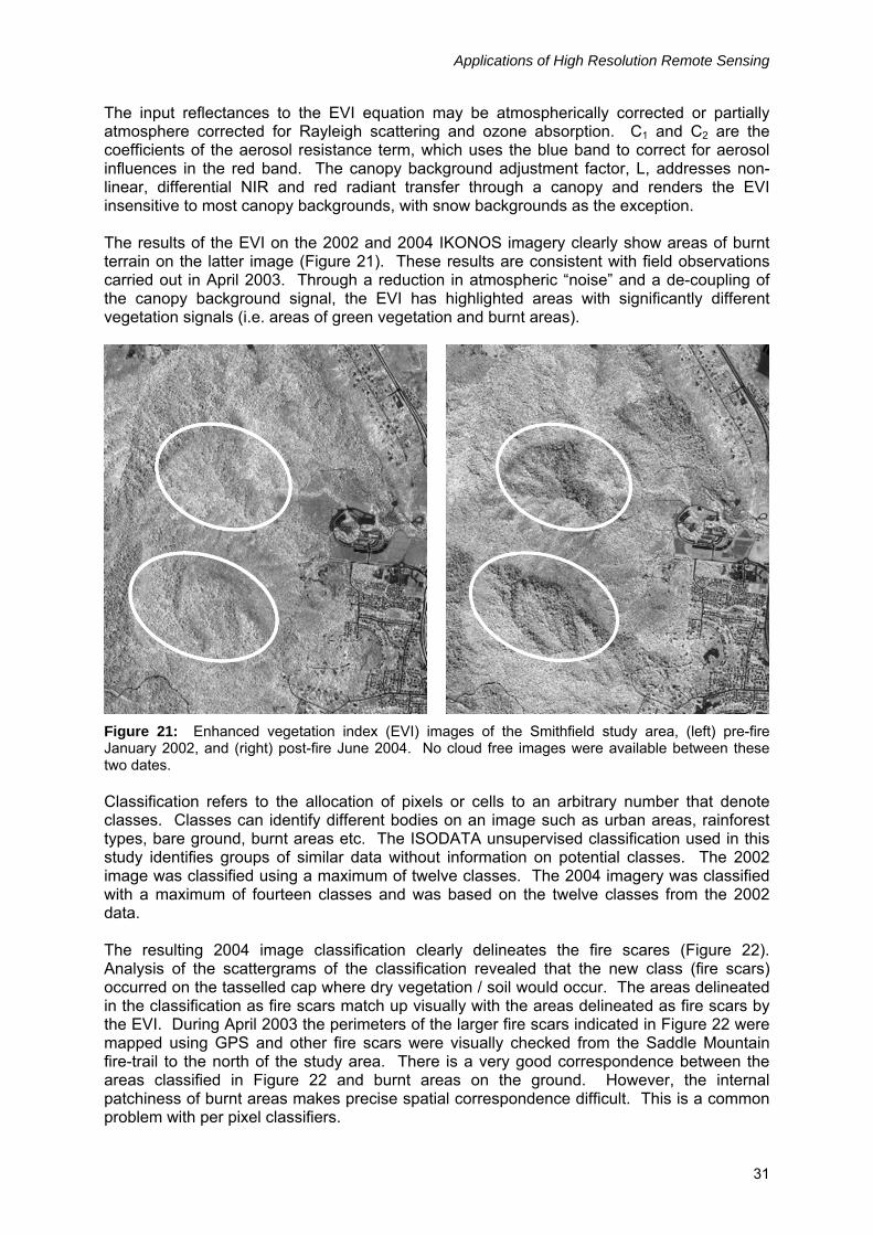
The input reflectances to the EVI equation may be atmospherically corrected or partially atmosphere corrected for Rayleigh scattering and ozone absorption. C1 and C2 are the coefficients of the aerosol resistance term, which uses the blue band to correct for aerosol influences in the red band. The canopy background adjustment factor, L, addresses non-linear, differential NIR and red radiant transfer through a canopy and renders the EVI insensitive to most canopy backgrounds, with snow backgrounds as the exception. The results of the EVI on the 2002 and 2004 IKONOS imagery clearly show areas of burnt terrain on the latter image (Figure 21). These results are consistent with field observations carried out in April 2003. Through a reduction in atmospheric “noise” and a de-coupling of the canopy background signal, the EVI has highlighted areas with significantly different vegetation signals (i.e. areas of green vegetation and burnt areas).
Figure 21: Enhanced vegetation index (EVI) images of the Smithfield study area, (left) pre-fire January 2002, and (right) post-fire June 2004. No cloud free images were available between these two dates. Classification refers to the allocation of pixels or cells to an arbitrary number that denote classes. Classes can identify different bodies on an image such as urban areas, rainforest types, bare ground, burnt areas etc. The ISODATA unsupervised classification used in this study identifies groups of similar data without information on potential classes. The 2002 image was classified using a maximum of twelve classes. The 2004 imagery was classified with a maximum of fourteen classes and was based on the twelve classes from the 2002 data. The resulting 2004 image classification clearly delineates the fire scares (Figure 22). Analysis of the scattergrams of the classification revealed that the new class (fire scars) occurred on the tasselled cap where dry vegetation / soil would occur. The areas delineated in the classification as fire scars match up visually with the areas delineated as fire scars by the EVI. During April 2003 the perimeters of the larger fire scars indicated in Figure 22 were mapped using GPS and other fire scars were visually checked from the Saddle Mountain fire-trail to the north of the study area. There is a very good correspondence between the areas classified in Figure 22 and burnt areas on the ground. However, the internal patchiness of burnt areas makes precise spatial correspondence difficult. This is a common problem with per pixel classifiers.

Gillieson, Lawson and Searle
32
Figure 22: Classified images (isodata algorithm for the Smithfield study area):
(left) pre-fire January 2002, and (right) post-fire June 2004, fire scars shown in purple. Due to the nature of fire behaviour in a rainforest setting, current mapping techniques using NOAA or MODIS imagery are unsuitable. Fires in rainforests are generally small (<20 ha) and thus undetectable by this coarse spatial resolution imagery. Multitemporal IKONOS imagery, with its high resolution, is very useful in detecting fire scars in the tropical rainforests of North Queensland. The high resolution (4 m multispectral and 1 m spatial cells) of the imagery allows for the discrimination of fire scars on a much finer scale than NOAA or MODIS. However a number of image processing procedures must be employed before the imagery can be used to successfully to discriminate between burnt and unburnt land. The Enhanced Vegetation Index (EVI) was used to delineate areas of burnt country. It does this by using a formula involving the red, blue, and near infra-red bands which detect chlorophyll and thus as vegetation that has been burnt does not contain any chlorophyll, different reflectance values are given to burnt and unburnt vegetation. This successfully correlated with on-ground inspections. This type of mapping can be used on a local scale to more accurately assess the impacts of fire on rainforested areas. 3.5 ASSESSING THE HEALTH OF RIPARIAN RAINFORESTS IN
THE MOSSMAN CATCHMENT
Mediating between water and land, riparian zones are amongst the most dynamic natural systems in the landscape (Harris 1984; Croonquist and Brooks 1991; Gregory et al. 1991; Hancock et al. 1996) and can be thought of as temporal and spatial patterns of aquatic ecosystems, terrestrial plant succession and hydrologic and geomorphic processes (Gregory et al. 1991). Existing in such a dynamic part of the landscape, riparian zones are constantly undergoing change bought about by natural processes (Tubman and Price 1999). These may come in the form of periodic floods, irregular cyclones, wildfires, and on a smaller scale tree falls and bank collapse, all of which can result in vegetation changes and increased erosion. Over the last 150 years the disturbance regime has been dramatically changed by anthropogenic activities such as clearing, resulting in fragmentation of the landscape and reduced functionality of many riparian zones. In dynamic tropical landscapes with high
Applications of High Resolution Remote Sensing
33
natural variability in disturbance regimes, human impacts must be evaluated against the long-term record of environmental change to reliably assess their ecological effects (Landres et al. 1999). GIS and remote sensing techniques have been used in many areas to assess vegetation change over time (Mosugelo et al. 2002; Rhemtulla et al. 2002; Narumalani et al. 2004; Bouma and Kobryn 2004). The role of historical data is increasingly becoming an important measure in the fields of ecosystem management and restoration ecology (Swetnam et al. 1999; Landres et al. 1999). These historical data can provide the necessary baseline environmental conditions or data upon which a greater understanding for an ecosystem type can be gained and thus management of that ecosystem can be enhanced (Swetnam et al. 1999). This study was undertaken on the coastal lowlands of the Douglas Shire in the Wet Tropics bioregion of northern Queensland, Australia. The area has been heavily transformed for agricultural purposes, predominantly sugar cane production. A large proportion of the remaining vegetation consists of riparian rainforest, the focus of the study. The study area (Figure 23) was located in the vicinity of the town of Mossman (16.27.0S latitude, 145.23.0E longitude). The Mossman River is the major watercourse in this catchment with the South Mossman River and Cassowary Creek being its two major tributaries (Burrows 1998). The well-drained alluvial soils of the floodplains of the three watercourses (Murtha 1989), support rainforest vegetation types including Complex Mesophyll Vine Forest (type 1a) and Mesophyll Vine Forests (type 2a, type 3a sensu Tracey 1982) (Werren 1993). Traditional remote sensing products such as aerial photography can be analysed using the new software tools developed for digital image analysis and GIS. This is advantageous when historical images predate the introduction of digital formats. Conversion to digital images, rectification to a map base and integration within GIS allows detailed analysis of landscape change. In this study, changes in the extent of riparian vegetation along the Mossman River, South Mossman River and Cassowary Creek catchments were assessed using aerial photography from 1944 and 2000. The oldest aerial photography available was flown in September 1944 by the Royal Australian Air Force (RAAF) at a scale of approximately 1:24,600 (greyscale). The more recent set of colour photos were flown in August 1998 and 2000 at a scale of approximately 1:25,000 (Table 7). Both sets of photos were ortho-rectified and mosaiced using ER-Mapper 6.4 and OrthoWarp 2.3 software. A digital elevation model (DEM) with 10 m cells was used in ortho-rectification. Ground control points (GCP) were gained from GIS layers of roads and streams, combined with additional points gained by field survey using differential GPS. The extent of the riparian vegetation along the Mossman River, South Mossman River and Cassowary Creek was digitised on-screen on the 1944 dataset, working at a scale of approximately 1:3,500. This digitised layer was then overlain on the 2000 mosaic and areas of vegetation loss or gain were identified and digitised. Areas of vegetation thickening (regrowth) were also digitised together with areas that showed no difference in the extent of the riparian vegetation (within error limits) between the two dates. Consequently four new GIS layers were created and were used to produce a final map (Figure 24) highlighting the change in extent of the riparian vegetation along the Mossman River, the South Mossman River and Cassowary Creek between 1944 and 2000.

Gillieson, Lawson and Searle
34
Figure 23: Location of study area watercourses around the town of Mossman, North Queensland.
The use of repeat aerial photography in this study showed that during the 56-year period, a total of 285 hectares of riparian forest changed in its extent (Table 7 and Figure 24). Of this change approximately 124 hectares were gained and 102 hectares were lost. This resulted in a net gain of 22 hectares of riparian rainforest along the three watercourses. A further 59 hectares of forest became obviously thicker in its cover over this time period. Differences in riparian vegetation extent were identified as either a result of clearing, changes in farm management practices or stream channel movement.
Applications of High Resolution Remote Sensing
35
Table 7: Total change in extent of riparian rainforest in the Mossman Catchment between 1944 and 2000.
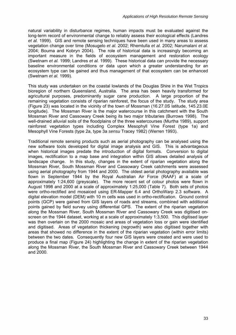
Change Area in hectares Percentage of total change
Loss 102 35.79
Thickening 59 20.70
Gain 124 43.59
Total 285 100 The coastal lowlands in this region have been under immense pressure for the development of agricultural activities due to reliable rainfall and high soil fertility. Subsequently large tracts of rainforest have been cleared to facilitate these activities (Figure 24) (Winter et al. 1987). Where forests existed in the mid 1940s but in 2000 had been developed for agricultural production, clearing was identified as the major cause of change in riparian forest extent. Within the study area, most of this type of vegetation change has occurred in two large areas, one towards the headwaters of the Mossman River and the other towards the mouth of the Mossman River. There are many smaller patches of riparian vegetation loss along all watercourses that may be attributed to clearing. This change has resulted in the loss of approximately 92 ha of riparian vegetation in the study area between 1944 and 2000. Changes in the extent of riparian vegetation in this catchment may also be a result of changing farm management practices (Figure 25), namely a reduction in sugarcane burning. Prior to the 1930s, cane crops were mostly unburnt, however during the mid 1930s pre-harvest burning of cane was a common practice in Queensland cane fields (King et al. 1953; Penrose 1998). Fire was used as a harvesting and pest and disease management tool. Burning cane resulted in the reduction of the amount of weeds, leaves and other matter that could potentially impede the harvesting and milling processes (Queensland Sugar Corporation 1995). Cane fires, whether as a means of harvesting management or pest and disease control, were not contained and allowed to continue until they burnt out. The fires generally burnt out on hill slopes surrounding the cane farms. Due to prolonged wet periods in the early to mid 1970s and the advent of mechanical harvesting, green harvesting was adopted by many cane farmers in the area (Ridge et al. 1979; Baxter 1983), hence cane burning reduced dramatically. As a result of green harvesting, and subsequent reduction in uncontained cane fires, native rainforest began to expand down the hill slopes and along the watercourses. This regrowth forms much of the forest seen in the area today. This type of change generally occurs where cane farms bound the riparian vegetation and rainforest covered hillsides. This type of change has resulted in the gain of approximately 110 ha in table and the thickening of approximately 55 ha of hill slope and riparian vegetation in the study area (Figure 24). Riparian vegetation modifies channel morphology by trapping sediment or altering channel hydraulics (Naiman and Décamps 1997). During a flood event the accretion of sediment by vegetation may be substantial, resulting in a possible redirection of the flow and the movement or retention of material (Naiman and Décamps 1997). Large woody debris (LWD) (added to the stream via the riparian vegetation) or roots may alter the channel hydraulics by influencing waterpower and/or flow and current direction. LWD and roots may also trap and hold material, which may cause the water to erode parts of the bank at higher rates than previously experienced. This may result in mass movement of sediment and deposition in areas where it previously did not occur (Naiman and Décamps 1997).

Gillieson, Lawson and Searle
36
Figure 24: Changes in riparian vegetation, Mossman catchment 1944-2000.
Changes in Riparian Vegetation Extent in the Mossman Catchments between 1944 and 2000
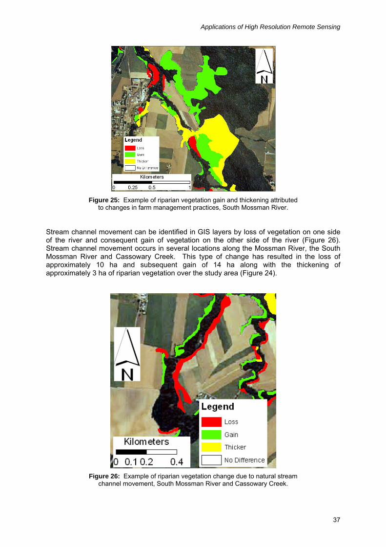
Applications of High Resolution Remote Sensing
37
Figure 25: Example of riparian vegetation gain and thickening attributed
to changes in farm management practices, South Mossman River. Stream channel movement can be identified in GIS layers by loss of vegetation on one side of the river and consequent gain of vegetation on the other side of the river (Figure 26). Stream channel movement occurs in several locations along the Mossman River, the South Mossman River and Cassowary Creek. This type of change has resulted in the loss of approximately 10 ha and subsequent gain of 14 ha along with the thickening of approximately 3 ha of riparian vegetation over the study area (Figure 24).
Figure 26: Example of riparian vegetation change due to natural stream
channel movement, South Mossman River and Cassowary Creek.
Gillieson, Lawson and Searle
38
In tropical areas where baseline ecological data are frequently missing, GIS and aerial photographic analyses can be useful if an adequate time-series of images is available (Parsons et al. 1999). The change in extent of riparian vegetation along the Mossman, South Mossman and Cassowary creek watercourses was assessed to gain an understanding of historic riparian vegetation patterns. This showed that both anthropogenic activities (clearing and changing land management practices) and natural processes (stream channel movement) have influenced the extent of riparian vegetation in this area. The habitat quality value of the riparian zone will be affected by these extent changes. Rainforest-dependent birds and total species richness will be impacted upon by changes that result in a reduction of canopy cover. Thus to maintain and enhance the value of riparian zones as habitat for both flora and fauna an understanding of the processes that influence the quality of the vegetation in these zones is essential. This will aid future planning and lead to the application of more suitable land management practices. There is now a clear and objective view of where changes have occurred in the riparian vegetation between the two dates and this may be used as a template to model natural vegetation change in the future. Knowing the types of vegetation that existed along the watercourses in the past may help revegetation programs in the future by giving them a base from which to work, when combined with vegetation descriptions currently available (Tracey 1982).

Applications of High Resolution Remote Sensing
39
4. CONCLUSIONS The choice of remotely sensed data for ecological applications in rainforest areas and for management studies will ultimately depend on precise formulation of research questions and careful evaluation of the necessary spatial, spectral and radiometric resolution thus required. There are many potential candidates amongst a galaxy of sensors and satellites. Factors of price and availability cannot be discounted, especially in tropical regions where persistent cloud cover can thwart efforts to obtain cloud-free imagery for particular dates and months of any year. There has also been a shift from low cost, government-sponsored sensors to higher cost, commercial sensors over the last decade. Maintaining access to the data for a particular sensor may be a problem given the volatility of the commercial scene, with many company mergers and an evolving trend to restrictions on data access for strategic reasons. It is now possible to remotely sense many forest structural parameters and some plant physiological parameters using high resolution remote sensing. All of these require detailed ground verification of both deterministic and empirical models, adding to the cost of any project. It may be that these models are specific for a particular rainforest type, but robust methodologies should be adaptable to different settings. The methodologies for remote sensing of land use change, forest clearance and fragmentation are now well established at a variety of spatial scales, and some are becoming routine operational tools for land managers. But there is a real need for adequate training for land managers in remote sensing techniques, especially in developing countries and also in more remote regions of developed countries. The challenges remaining for researchers are to evaluate new image classification methodologies, such as object oriented classifiers, to rainforest environments and to further refine the models that relate forest structural and physiological parameters to remotely sensed data. For managers, there needs to be an acceptance of what remote sensing can and cannot do in evaluating environmental impacts and land use change. Thus researchers and managers need to form strategic alliances to guide research and to inform government policy on remote sensing and its applications.


Applications of High Resolution Remote Sensing
41
REFERENCES Adams, J. B., Sabol, D. E., Kapos, V., Filho, R. A., Roberts, D. A., O., S. M. and Gillespie, A. R. (1995). Classification of Multispectral Images Based on Fractions of Endmembers: Application to Land-Cover Change in the Brazilian Amazon. Remote Sensing of the Environment 52: 137-154. Aplin, P. (2003). Remote sensing: base mapping. Progress in Physical Geography 27: 275-283. Asner, G. P., Palace, M., Keller, M., Pereirs Jr., R., Silva, J. N. M. and Zweede, J. C. (2002). Estimating canopy structure in an Amazon forest from laser range finder and IKONOS satellite observations. Biotropica 34: 483-492. Baxter, B. (1983). Green cane harvest review. Australian Canegrower February: 32-35. Bouma, G. A. and Kobryn, H. T. (2004). Change in vegetation cover in East Timor, 1989-1999. Natural Resources Forum 28: 1-12. Brown, B. (1999). Occurrence and impact of Phytophthora cinnamomi and other Phytophthora species in rainforests of the Wet Tropics World Heritage Area. pp. 41-76 In: Gadek, P. (ed.) Patch Deaths in Tropical Queensland Rainforests: Association and Impact of Phytophthora cinnamomi and Other Soil Borne Organisms. Rainforest CRC, Cairns. Brown, B. N. (1976). Phytophthora cinnamomi associated with patch death in tropical rain forests in Queensland. Australian Plant Pathology Society Newsletter 5: 1-4. Burrows, D. W. (1998). FNQ 2010 Regional Environmental Strategy – Key Waterways Report. Australian Centre for Tropical Freshwater Research, James Cook University, Townsville. Chester, G., Goosem, M., Cowan, J., Harriss, C. and Tucker, N. (2006). Roads in Tropical Forests - Best Practice Guidelines. Unpublished report by the Cooperative Research Centre for Tropical Rainforest Ecology and Management (Rainforest CRC) for the Queensland Department of Main Roads. Clark, D. B., Castro, C. S., Alvarado, L. D. A. and Read, J. M. (2004). Quantifying mortality of tropical rainforest trees using high-spatial-resolution satellite data. Ecology Letters 7: 52-59. Cochrane, M. A. (2003). Fire science for rainforests. Nature 421: 919-919. Cochrane, M. A. (2001). Synergistic interactions between habitat fragmentation and fire in evergreen tropical forests. Conservation Biology 15: 1515-1521. Cochrane, M. A. and Schulze, M. D. (1999). Fire as a recurrent event in tropical forests of the eastern Amazon: Effects on forest structure, biomass, and species composition. Biotropica 31: 2-16. Cochrane, M. A. and Schulze, M. D. (1998). Forest fires in the Brazilian Amazon. Conservation Biology 12: 948-950. Croonquist, M. J. and Brooks, R. P. (1991). Use of avian and mammalian guilds as indicators of cumulative impacts in riparian-wetland areas. Environmental Management 15: 701-714.

Gillieson, Lawson and Searle
42
Dial, G. and Grodecki, J. (2003). Applications of IKONOS imagery. ASPRS Annual Conference Proceedings. Anchorage, Alaska. Dwyer, E., Gregoire, J. M. and Malingreau, J. P. (1998). A Global Analysis of Vegetation Fires Using Satellite Images: Spatial and Temporal Dynamics. Ambio 27: 175-181. Forman, R. T. T. and Alexander, L. E. (1998). Roads and their major ecological effects. Annual Review of Ecology and Systematics 29: 207 231. Forman, R. T., Sperling, D., Bissonette, J. A., Clevenger, A. P., Cutshall, C. D., Dale, V. H., Fahrig, L., France, R., Goldman, C. R., Heanue, K., Jones, J. A., Swanson, F. J., Turrentine, T. and Winter, T. C. (2003). Road Ecology – Science and Solutions. Island Press, Washington. Gillieson, D., Landsberg, J., Gadek, P. and Edwards, W. (2002). Mapping and environmental correlates of canopy dieback in rainforests, Wet Tropics World Heritage Area. In: Holland, P. (ed.). 2001 A Spatial Odyssey, Proceedings IAG-NZGS Conference. University of Otago, Dunedin, February 2001. Ginsberg, J. R. (1998). Perspectives on wildfire in the humid tropics. Conservation Biology 12: 942-943. Goetz, S. J., Wright, R. K., Smith, A. J., Zinecker, E. and Schaub, E. (2003). IKONOS imagery for resource management: Tree cover, impervious surfaces, and riparian buffer analysis in the mid-Atlantic region. Remote Sensing of Environment 88: 195-208. Goosem, M. (2000). Effects of tropical rainforest roads on small mammals: edge changes in community composition. Wildlife Research 27: 151-163. Goosem, M. (2002). Effects of tropical rainforest roads on small mammals: fragmentation, edge effects and traffic disturbance. Wildlife Research 29: 277-289. Goosem, M. (2003). East Evelyn faunal underpass effectiveness. In: Proceedings of the National Environment Conference, Brisbane, June 2003. CD-ROM. Environmental Engineering Society, Brisbane. Goosem, S. and Tucker, N. (1995). Repairing the Rainforest. Wet Tropics Management Authority, Cairns. Goosem, S. (2000). The Wet Tropics landscape, ecology and values. In: Lane, M. and McDonald, G. (eds.) Securing the Wet Tropics: a retrospective on managing Australia’s tropical rainforest. Federation Press, Sydney. Gregory, S. V., Swanson, F. J., McKee, W. A. and Cummins, K. W. (1991). An ecosystem perspective of riparian zones. BioScience 4: 540-552. Hancock, C. N., Ladd, P. G. and Froend, R. H. (1996). Biodiversity and management of riparian vegetation in Western Australia. Forest Ecology and Management 85: 239-250. Harris, L. D. (1984). The Fragmented Forest: Island Biogeography Theory and the Preservation of Biotic Diversity. The University of Chicago Press, Chicago. Kayitakire, F., Farcy, C. and Defourny, P. (2002). IKONOS-2 imagery potential for forest stands mapping. Presented at ForestSAT Symposium Heriot Watt University, Edinburgh.

Applications of High Resolution Remote Sensing
43
Kershaw, P., Moss, P. and Van der Kaars, S. (2003). Causes and consequences of long-term climatic variability on the Australian continent. Freshwater Biology 48: 1274-1283. King, N. J., Mungomery, R. W. and Hughs, C. G. (1953). Manual of cane-growing. Angus and Robertson. Sydney, Australia. Kinnaird, M. F. and O’Brian, T. G. (1998). Ecological effects of wildfire on lowland rainforest in Sumatra. Conservation Biology 12: 954-956. Landres, P. B., Morgan, P. and Swanson, F. J. (1999). Overview of the use of natural variability concepts in managing ecological systems. Ecological Applications 9: 1179-1188. Laurance, S. G. W., Stouffer, P. C., Laurance, W. F. (2004). Effects of road clearings on movement patterns of understory rainforest birds in central Amazonia. Conservation Biology 18: 1099–1109. Law, K. H. and Nichol, J. (2004). Topographic correction for differential illumination effects on IKONOS satellite imagery. International Archives of Photogrammetry Remote Sensing and Spatial Information Sciences 35: 641-646. Lawson, T., Goosem, M. and Gillieson, D. (in review). Rapid assessment of habitat quality in riparian rainforest vegetation. Pacific Conservation Biology. Margules, C. R. and Pressey, R. L. (2000). Systematic conservation planning. Nature 405: 243-253. Marrinan, M. J., Edwards, W. and Landsberg, J. (2005). Resprouting of saplings following a tropical rainforest fire in north-east Queensland, Australia. Austral Ecology 30: 817-826. McDonald, E. R. (2005). Using UML to improve spatial software development. Proceedings of SSC 2005 Spatial Intelligence, Innovation and Praxis: the national biennial Conference of the Spatial Sciences Institute. Melbourne. Mosugelo, D. K., Moe, S. R., Ringrose, S. and Nellemann, C. (2002). Vegetation changes during a 36-year period in northern Chobe National park, Botswana. African Journal of Ecology 40: 232-240. Murtha, G. G. (1989). Soils of the Mossman Cape Tribulation Area, North Queensland. CSIRO, Australia. Naiman, R. J. and Décamps, H. (1997). The ecology of interfaces: Riparian zones. Annual Review of Ecology and Systematics 28: 621-658. Narumalani, S., Mishra, D. R. and Rothwell, R. G. (2004). Analysing landscape structural change using image interpretation and spatial pattern techniques. Mapping Sciences and Remote Sensing 41: 25-44. Nepstad, D. C., VerõÂssimo, A., Alencar, A., Nobre, C., Lima, E., Lefebvre, P., Schlesinger, P., Potter, C., Moutinho, P., Mendoza, E., Cochrane, M. and Brooks, V. (1999). Large-scale impoverishment of Amazonian forests by logging and fire. Nature 398: 505-508. Parsons, D. Swetnam, T. W. and Christensen, N. L. (1999). Uses and limitations of historical variability concepts in managing ecosystems. Ecological Applications 9: 1177-1178.
Gillieson, Lawson and Searle
44
Penrose, B. (1998). Medical experts and occupational illness: Weil’s disease in North Queensland, 1933-1936. Labour History 75: 125-143. Phinn, S. R., Stanford, M. and Held, A. (2000). Remote Sensing Requirements for Management Agencies Responsible for Forest and Water Quality Monitoring in the Wet Tropics. Rainforest CRC, Cairns. Queensland Sugar Corporation (1995). Australian sugar notes. Queensland Sugar Corporation, Brisbane. Raino, D., Chuvieco, E., Salas, J. and Aguado, I. (2003). Assessment of different topographic corrections in Landsat-TM data for mapping vegetation types. IEEE Transactions on Geoscience and Remote Sensing 41: 1056-1061. Rhemtulla, J. M., Hall, R. J., Higgs, E. S., and Macdonald, S. E. (2002). Eighty years of change: vegetation in the montane ecoregion of Jasper National Park, Alberta, Canada. Canadian Journal of Forest Research 32: 2010-2021. Ridge, D., Hurney, A. and Chandler, K. (1979). Trash disposal after green cane harvesting. Proceedings of the Australian Society of Sugar Cane Technologists 1: 89-92. Roberts, D. A., Batista, G., Pereira, J., Waller, E., and Nelson, B. (1998). Change identification using multitemporal spectral mixture analysis: Applications in Eastern Amazonia. In: Elvidge, C. and Lunetta, R. (eds.) Remote sensing change detection: Environmental monitoring applications and methods, Chapter 9, pp. 137-161. Ann Arbor Press, Ann Arbor. Siegert, F. and Hoffmann, A. A. (2000). The 1998 forest fires in East Kalimantan (Indonesia): A quantitative evaluation using high resolution, multitemporal ERS-2 SAR images and NOAA-AVHRR hotspot data. Remote Sensing of Environment 72: 64-77. Siegert, F., Ruecker, G., Hinriches, A. and Hoffmann, A. A. (2001). Increased damage from fires in logged forests during droughts caused by El Nino. Nature 414: 437-440. Souza Jr., C. M. and Roberts, D. (2005). Mapping forest degradation in the Amazon region with IKONOS images. International Journal of Remote Sensing 26: 425-429. Space Imaging (accessed March to April 2006). Calibration of IKONOS imagery to at-aperture, in-band radiance. IKONOS planetary reflectance and mean solar exoatmospheric irradiance. www.spaceimaging.com Spellerberg, I. F. (1998). Ecological effects of roads and traffic: a literature review. Global Ecology and Biogeography Letters 7: 317 – 313 Stanton, P. and Stanton, D. (2003). Various Map Sheet Reports. Unpublished reports to the Wet Tropics Management Authority, Cairns. Swetnam, T. W., Allen, C. D. and Betancourt, J. L. (1999). Applied historical ecology: Using the past to manage for the future. Ecological Applications 9: 1189-1206. Teillet, P. M., Guindon, B. and Goodenough, D. G. (1982). On the slope-aspect correction of multispectral scanner data. Canadian Journal of Remote Sensing 8: 84-106. Terrestrial Biophysics and Remote Sensing Lab (accessed March to April 2005) http://tbrs.arizona.edu/cdrom/Index.html
Applications of High Resolution Remote Sensing
45
Timmerman, A., Oberhuber, J., Bacher, A., Esch, M., Latiff, M. and Roeckner, E. (1999). Increased El Nino frequency in a climate model forced by future greenhouse warming. Nature 398: 694-697. Tracey, J. G. (1982). The vegetation of the humid tropical region of north Queensland. CSIRO, Melbourne. Tracey, J. G. and Webb, L. J. (1975). 1:100 000 Maps of the Humid Tropical Region of North Queensland. CSIRO, Queensland. Trott, L. and Goosem, S. (1996). Wet Tropics in Profile. Wet Tropics Management Authority, Cairns. Tubman, W. and Price, P. (1999). The significance and status of riparian land. In: Lovett, S. and Price, P. (eds.), Riparian Land Management Technical Guidelines. Volume One: Principles of Sound Management. Land and Water Resources Research and Development Corporation, Canberra. Uhl, C. and Kauffman, J. B. and Cummings, D. L. (1988). Fire in the Venezuelan Amazon 2: Environmental conditions necessary for forest fires in the evergreen rainforest of Venezuela. Oikos 53:176-184. Uhl, C. and Kauffman, J. B. (1990). Deforestation, fire susceptibility, and potential tree responses to fire in the Eastern Amazon. Ecology 71: 437-449. Werren, G. (1993). Conservation values of ‘unprotected’ lands within the Lower Daintree, Mossman and Mowbray River Catchments, Douglas Shire: Contribution to the Douglas Shire River Improvement Trust Scoping Study. James Cook University, Cairns. Wet Tropics Management Authority (1999). Wet Tropics Research Strategy. WTMA, Cairns. White, J. C., Wulder, M. A., Brooks, D., Reich, R. and Wheate, R. D. (2005). Detection of red attack stage mountain pine beetle infestation with high spatial resolution satellite imagery. Remote Sensing of Environment 96: 340-351. Winter, J. W., Bell, F. C. and Pahl, L. I. (1987). Rainforest clearfelling in northeastern Australia. Proceedings of the Royal Society of Queensland 98: 41-57.