application of multiphase transport models to field remediation by air sparging and soil vapor...

A

ooiaaorthmtbcr©

K

1

R[nnmtoa

0d

Journal of Hazardous Materials 143 (2007) 156–170

Application of multiphase transport models to field remediationby air sparging and soil vapor extraction

M.E. Rahbeh a, R.H. Mohtar b,∗a Department of Renewable Resources, University of Alberta, Edmonton, Alberta, Canada

b Department of Agricultural Engineering, Purdue University, 225 South University Street, West Lafayette, IN, United States

Received 13 September 2004; received in revised form 26 June 2006; accepted 4 September 2006Available online 9 November 2006

bstract

The design and operation of air sparging and soil vapor extraction (AS/SVE) remediation systems remains in large an art due to the absencef reliable physically based models that can utilize the limited available field data. In this paper, a numerical model developed for the design andperation of air sparging and soil vapor extractions systems was used to simulate two field case studies. The first-order mass transfer kinetics werencorporated into the model to account for contaminant mass transfer between the water and air (stripping), NAPL and water (dissolution), NAPLnd air (volatilization), and water and soil (sorption/desorption), the model also accounted for soil heterogeneity. Benzene, toluene, ethyl benzenend xylenes (BTEX) were the contaminants of concern in both case studies. In the second case study, the model was used to evaluate the effectf pulsed sparging on the removal rate of BTEX compounds. The pulsed sparging operation was approximated assuming uniform contaminantedistribution at the beginning of the shut-off period. The close comparison between the observed and simulated contaminant concentration inhe aqueous phase showed that the approximation of the pulsed sparging operation yielded reasonable prediction of the removal process. Fieldeterogeneity was simulated using Monte Carlo analysis. The model predicted about 80–85% of the contaminant mass was removed by air–waterass transfer, which was similar to the average removal obtained by Monte Carlo analysis. The analysis of the removal/rebound cycles demonstrated

hat removal rate was controlled by the organic–aqueous distribution coefficient Koc. Due to the lack of site-specific data, the aerobic first-orderiodegradation coefficients (kbio) were obtained from a literature survey, therefore, uncertainty analysis of the kbio was conducted to evaluate theontribution of the aerobic biodegradation to total contaminant removal. Results of both case studies showed that biodegradation played a majorole in the remediation of the contaminated sites.

2006 Elsevier B.V. All rights reserved.

reme

pmmcuPdi

eywords: Air sparging; Biodegradation; Pulsed sparging; Mass transfer; Field

. Introduction

The introduction of the Comprehensive Environmentalesponse, Compensation, and Liability Act (CERCLA) of 1980

1] created the need for the evaluation and treatment of contami-ant plumes caused by accidental spills of industrial waste. Theeed for multiphase flow and transport models became evenore pressing after the development of remediation techniques

hat require the injection of remedial fluids such as co-solvents,
r techniques that involve remediation by advective air flux suchir sparging (AS) and/or soil vapor extraction (SVE).
∗ Corresponding author. Tel.: +1 765 494 1791; fax: +1 765 496 1115.E-mail address: [email protected] (R.H. Mohtar).

caefaAp

304-3894/$ – see front matter © 2006 Elsevier B.V. All rights reserved.oi:10.1016/j.jhazmat.2006.09.098

diation

Multiphase flow and transport modeling is a well-knownractice in the petroleum engineering, however, the differentotivation of the petroleum and environmental engineering pro-oted the development of models that are generally aimed at the

haracterization of the contaminant plume [2–5], and the sim-lation and design of remediation systems [6–10]. Abriola andinder [11] demonstrated their model [2] by modelling the one-imensional hypothetical infiltration of a hydrocarbon mixturento a soil column. Sleep and Sykes [12] considered a hypotheti-al distribution of organic contaminant in the subsurface. Baehrnd Corpcioglu [13] used a one-dimensional approximation tovaluate, hypothetically, the transport of organic contaminant
rom the unsaturated zone into ground water. Unger et al. [8]nd Rathfelder et al. [10] applied their models to hypotheticalS/SVE problems. All of these models and research articlesrovided an excellent discussion and insight for the numerical
mailto:[email protected]

dx.doi.org/10.1016/j.jhazmat.2006.09.098

f Haza

st[eatat

eiaactoans

2

2

uafpiaItmitatacsanTrmgafim

2

uf(d

bhafamflvbFtMTsnfe

2

mtTfiwtiatpbetmt(tbtstt

2

seii

t

M.E. Rahbeh, R.H. Mohtar / Journal o

olution of multiphase systems, however, without applicationo field case studies, Radideau et al. [14] and Benner et al.15] applied semi-empirical models to field case studies. Semi-mpirical models, however, require an on-site pre-calibration ofn existing air sparging system before it can be used. In this case,he model cannot be used for the design and feasibility studies,nd cannot be used for short-term operations, which may defeathe purpose of the model in the first place.

Our objective is to demonstrate the use of a practical andfficient model in the evaluation of two AS/SVE field case stud-es. The main advantage of the model is its flexibility to takedvantage of the limited amount of data that are usually avail-ble, while retaining the ability to simulate the processes thatontribute to the overall contaminant removal. The analysis forhe first case study focuses on the effect of natural attenuationn the contaminant removal processes. The second case studyddresses the issues of heterogeneity and pulse sparging, a tech-ique that is usually used to enhance the performance of ASystems.

. Methodology

.1. Model description

The unsaturated air flow and contaminant transport modelses first-order kinetics to represent the mass transfer among thequeous, gaseous, solid, and NAPL phases. The model accountsor heterogeneous domains and considers distinguished single-hase and multi-phase domains. This capability is especiallymportant in the case of remediation techniques that involve andvective air flux such as air sparging and soil vapor extraction.n such systems, two domains may be considered, the advec-ive domain, i.e. the air, and the non-advective domain, which

ay be either the domain outside the advective air domain butn the vicinity of the air-plume, or any space or pocket insidehe advective air domain that is not in direct contact with thedvective air domain. The model consists of two main modules;he first module, the steady state unsaturated flow that solves forir flow, uses air permeability as an input and determines theapillary pressure head distribution. The flow module can con-ider air injection (air sparging) by imposing positive pressures a fixed boundary condition at the sparging well. Likewise,egative pressure can be imposed to represent extraction (SVE).he second module, multiphase contaminant transport, incorpo-

ates first-order mass transfer kinetics to model the contaminantass transfer among all phases involved: namely, the aqueous,

aseous and, solid phases. The flow and transport simulationsre decoupled such that the steady state air flow is determinedrst, and then the pressure heads are interpolated to the transportodel.

.1.1. The steady unsaturated flow moduleAS and/or SVE are usually applied to remove trace and resid-

al contaminant concentrations rather than removing the NAPLree phase. In practice neither free flowing light non-aqueousLNAPL) nor dense non-aqueous phase (DNAPL) have beenetected at sites where an advective air flux technology has

rdous Materials 143 (2007) 156–170 157

een used as a remediation technique [16,17]. Furthermore, itas been found that the effect of ground water flow on the sizend shape of ROI is negligible [18], and that the time requiredor an AS to reach steady state is negligible relative to theverage operational time [16,18]. For SVE applications, Mass-ann [19] treated the air flow as saturated, i.e. single phaseow, by ignoring the effect of the soil moisture condition in theadose zone. Sawyer and Kamakoti [20], realizing the analogyetween flow equations, went one step further and used MOD-LOW as a design tool for SVE systems. In this paper, we used

he unsaturated steady state flow model SPARG, developed byohtar et al. [21], to supplement the transient multiphase model.

his involved the assumption of instantaneous attainment of theteady state conditions, which may incur some error at the begin-ing of simulation. However, it allowed independent simulationor the transport and flow components, thus saving substantialffort and computational time.

.1.2. Multiphase transport moduleThe multiphase contaminant transport model uses first-order

ass transfer kinetics, dC/dt = kf(C − Caq), to represent massransfer among the aqueous, gaseous, solid and NAPL phases.he theoretical basis of the multiphase transport model is

ounded on the concept that a polar liquid wets a polar surfacen preference to non-polar liquid, therefore, water preferentiallyets soil particles, thus preventing a direct contact between

he soil particles and intruding non-aqueous phase or advect-ng gaseous phase. This has been demonstrated by Wilson etl. [22] using etched glass micro models to visualize the dis-ribution of non-aqueous phase liquid (NAPL), water and airhases. They concluded that the glass was always surroundedy a thin film of water as the air and water were in contact withach other, but not with the glass which represented the soil par-icle in an actual porous medium. Therefore, the contaminant

ass transfer can take place across the aqueous–solid (sorp-ion/desorption), aqueous–gaseous (stripping), aqueous–NAPLdissolution), and gaseous–NAPL (volatilization) interfaces. Inhe context of remediation by AS/SVE, the mobile phases maye restricted to the aqueous and gaseous phases only. However,he model incorporates a seepage process in terms of a first-orderink term in order to relax the stationary aqueous phase assump-ion, and to compensate for the contaminant movement due tohe gentle slope in the water table.

.1.3. Governing equationsThe governing equations are based on the concept of con-

ervation of mass and volume averaging, or the representativequivalent volume (REV) [23], which has been extensively usedn multiphase contaminant transport models including thosenvolving an advective gaseous phase.

Accordingly, the governing equation for the contaminantransport in the aqueous phase is written as (e.g., Fetter [24]):

∂Cαaq

∂t= ∇Jα

aqi− Rα

stripping − Rαsoprtion/desorption + Rα

dissolution

− κCαaq − βCα

aq, i = 1, 2 (1)

1 f Haza

wCJttratir

p

w(Srmi

p

wη

d

p

wl(

o

∇

w

g

∇

wD

p

R

wfi

R

wfiid

R

wfiNc

R

w((

m

k

wi

fi

k

fi

k

wi

ts

l

TpiT

58 M.E. Rahbeh, R.H. Mohtar / Journal o

here i denotes the space dimension; α the contaminant type;aq the contaminant concentration in the aqueous phase (M/L3);

aq the contaminant flux in the aqueous phase (M/L2T); Rstrippinghe rate of mass transfer per unit volume per unit time acrosshe aqueous–gaseous interface (M/L3T); Rsorption/desorption theate of mass transfer per unit volume per unit time across thequeous–solid interface (M/L3T); Rdissolution the rate of massransfer per unit volume per unit time across the aqueous–NAPLnterface (M/L3T); κ the first-order bio-decay coefficient (1/T); βepresents the seepage process as the first-order sink term (1/T).

The governing equation for the contaminant in the gaseoushase is written as

∂cαg

∂t= ∇Jα

gi+ Saq

SgRα

stripping + Rαvolatilization, i = 1, 2 (2)

here cg is the contaminant concentration in the gaseous phaseM/L3); Jg the contaminant flux in the gaseous phase (M/L2T);aq the saturation of the aqueous phase (unitless); Sg the satu-ation of the gaseous phase (unitless); Rvolatilization is the rate ofass transfer per unit volume per unit time across the gas–NAPL

nterface (M/L3T).The governing equation for the contaminant on the solid

hase is written as

∂Sαs

∂t= ηSaq

ρbRα

sorption/desorption (3)

here Ss is the contaminant content in the solid phase (M/M);the porosity of the solid phase (unitless); ρb is the soil bulk

ensity (M/L3).The governing equation for the contaminant in the NAPL

hase is written as

∂XαNAPL

∂t= − Saq

θNAPLρNAPLRα

dissolution

− Sg

θNAPLρNAPLRα

volatilization (4)

here XNAPL is the non-aqueous phase volumetric fraction (unit-ess); θNAPL the non-aqueous phase initial residual saturationunitless);ρNAPL is the density of the non-aqueous phase (M/L3).

The governing equation for the contaminant flux in the aque-us phase is written as

Jαaq = ∂

∂xi

(Dα

aqi

∂Cαaq

∂xi

), i = 1, 2 (5)

here Daq is the aqueous phase diffusion coefficient (L2/T).The governing equation for the contaminant flux in the

aseous phase is written as

Jαg = −vg

∂cαg

∂x+ ∂

∂x

(Dα

gi

∂cαg

∂x

), i = 1, 2 (6)

i i i

here vg is the velocity of the advective gaseous phase (L/T);gi

is the hydrodynamic dispersion coefficient of the gaseoushase (L2/T).

o

∇

rdous Materials 143 (2007) 156–170

The mass transfer stripping term is written as

αstripping = ks

(Cα

aq − cαg

KαH

)(7)

here ks is the aqueous–gaseous first-order mass transfer coef-cient (1/T); and KH is the dimensionless Henry’s coefficient.

The mass transfer sorption/desorption term is written as

αsorption/desorption = kd

(Cα

aq − Sαs

KαD

)(8)

here kd is aqueous–solid the first-order mass transfer coef-cient; and KD is the aqueous–solid distribution coefficient;

t is a function of organic fraction (foc), and organic–aqueousistribution coefficient Koc; KD = focKoc (L3/M).

The mass transfer dissolution term is written as

αdissolution = kdis(χ

αnaqSolα − Cα

aq) (9)

here kdis is the NAPL–aqueous first-order mass transfer coef-cient (1/T); χnaq the contaminant molar fraction within theAPL composite (unitless); Sol is the solubility limit of theontaminant in the aqueous phase (M/L3).

The mass transfer volatilization term is written as

αvolitalization = kv(χα

naqVolα − cαg ) (10)

here kv is the NAPL–gas first-order mass transfer coefficient1/T); Vol is the equilibrium gaseous contaminant concentrationM/L3) referred to in this paper as volatility.

Accordingly, the aqueous–gaseous (stripping) first-orderass transfer coefficient is written as [25]:

s = 10−2.49D0.16mg v0.84

g d0.5550 K−0.61

H (11)

here Dmg is the diffusion coefficient of specific contaminantn the gaseous phase and d50 is the mean particle size (L).

The NAPL–air (volatilization) first-order mass transfer coef-cient is written as [26]:

v = 10−0.42D0.38mg v0.62

g d0.4450 (12)

The first-order NAPL–water (dissolution) mass transfer coef-cient is written as [27]:

dis = 10−2.69D1maqv

0.60aq d−0.73

50 (13)

here Dmaq is the diffusion coefficient of specific contaminantn the aqueous phase and vaq is the water velocity (L/T).

The solid–aqueous (sorption/desorption) first-order massransfer coefficient can be determined using the linear regressionuggested by Brusseau and Rao [28]:

og kd = 0.301 − 0.668 log kD (14)

he current model incorporates air flow and contaminant trans-ort processes. The numerical code for the air flow distributions derived from SPARG model developed by Mohtar et al. [21].heir model is based on a steady state unsaturated flow equation
f the form:(
kpkrg(Pc)

μg∇(Pc − ρgZ)

)= 0 (15)

f Haza

wpP(Zdpa

k

wpf

mfirictittissemmite(GfsotehiTiutmt

2

sttf

awaeatpobutpouatewnsoTmtata

3

3

nbuwtoamaomAt

fnwaTx


here kp is the intrinsic permeability (L2); krg the gaseoushase relative permeability (unitless); μ the viscosity (M/L/T2);c the capillary pressure head (M/L/T2); ρ the density

M/L3); ρ = ρaq − ρg; g the acceleration of gravity (L/T2);is the elevation head (L); and the subscripts ‘aq’ and ‘g’

enote the aqueous and gaseous phases, respectively. Theressure–permeability relationship is governed by the Brooksnd Corey [29] equation:

rg =(

1 −(

Pd

Pc

)λ)2(

1 −(

Pd

Pc

)2+λ)

(16)

here Pd is the entry air pressure head (M/L/T2) and λ is thearticle size distribution index [29]. Eq. (16) is a non-linearunction of Pc since the relative permeability is a function Pc.

A FORTRAN 90/95 code was developed using the finite ele-ent Galerkin formulation for spatial integration and centralnite difference scheme for time integration to solve for unsatu-ated air flow and multiphase contaminant transport. The modelnputs include initial condition, the chemical properties of theontaminants, and flow parameters. The model output includeshe capillary pressure distribution, from which the air flow veloc-ties can be calculated, and the contaminant concentration in allhe phases involved. The numerical solutions of partial differen-ial equations (PDE) usually result in sparse matrices; therefore,t is only sufficient to store the non-zero entries. This programtores the system of equations in a single vector, e.g. {A}. Theame routines are used to solve for the flow and transport tonsure efficient usage of storage and computational time. Theain modules may be categorized in four major groups: (1)odules to read the problem description, element and nodal

nformation, (2) modules used to determine the size of the sys-em of equations, (3) modules used to compose the system ofquations using the finite element-Galerkin’s formulation, and4) modules used to solve the system of equations using theauss–Siedel iterative technique, which is particularly suitable

or sparse matrices. These categories also signify the four majorteps that the program executes when solving either for air flowr multiphase contaminant transport. The possibility is retainedhat the mesh used for the transport problem may be differ-nt from that of the flow problem. In this case, the capillaryead distribution resulting from the flow module is interpolatednto the transport module using mesh interpolation subroutine.he sequential execution of the model first starts by reading the

nput data, which then is used to form the global matrix of thensaturated flow problem. After solving for the flow problemhe capillary heads are interpolated into the transport problem

esh, in turn the model forms the system of equations form theransport problem and solves it.

.2. Pulsed air sparging approximation

The finite element model described above consists of a
teady state unsaturated air flow module and a transient con-aminant transport module that incorporates first-order massransfer kinetics to simulate the inter-phase contaminant trans-er. To enable the model application to pulsed air sparging, we
fws

rdous Materials 143 (2007) 156–170 159

ssume that the mixing that occurs after each on and off cycleill be sufficient to produce uniform contaminant distribution

t the beginning of the following cycle, as suggested by Marleyt al. [30]. Thus, in addition to ignoring the transient stage ofir flow distribution, another error is incurred by ignoring theransient stage of the contaminant redistribution in the aqueoushase following the collapse of the radius of influence (ROI)f the air-plume. The assumption is advantageous, however,ecause it allows easy simulation of pulsed air sparging systemssing limited available field data. The validity of the assump-ion will be assessed by whether or not the model is capable ofredicting the contaminant removal within acceptable boundsf error, or within the field data measurement error. The sim-lation starts with an evenly distributed aqueous concentrationt the beginning of the air sparging cycle. At the beginning ofhe off cycle, the remaining contaminant mass is redistributedvenly in the zones that originally contained the contaminantithin the ROI. During the off cycle, changes in the contami-ant profile occur due to microbial and mass transfer processuch as sorption/desorption, and dissolution. The redistributionf the contaminant depends on the permeability of the flow field.he higher the permeability, the better is the redistribution andixing of the displaced water. AS/SVE systems are usually used

o remediate permeable soils, thus, the approximation of pulsedir sparging as discussed above is applicable under the condi-ions that are favorable to contaminant removal by an advectiveir flux.

. Air sparging case studies

.1. Porter County

The study area is located in northern Porter County, Indianaear the southern shore of Lake Michigan. The site was utilizedy a tin plate manufacturer; a small area of about 220 m2 wassed from 1980 till about 1987 as a drum storage area (DSA) forastes and organic chemicals used for the cleaning and main-

enance of tin plate sheets, mainly light LNAPL with a densityf approximately 0.85 g/cm3. The major constituents includedcetone (2-propanone), 2-butoxyethonal, 2-ethoxyethyl acetate,ethyl ethyl ketone (2-butanone), petroleum naphtha, toluene,

nd xylenes. The site became under scrutiny during the closuref the DSA; high levels of substituted benzenes, polycyclic aro-atic hydrocarbons, alkanes, and cycloalkane were identified.dditional soil and ground water investigations were undertaken

o determine the extent of the contamination [31].The study revealed that the soil and groundwater under the

ormer DSA contained xylenes, toluene, ethyl benzene, andaphthalene, and 2-mehylnaphthalene. The TEX compoundsere detected with regularity in the ground water. The toluene

nd xylene were above the EPA standard of MCL as shown inable 1. Therefore, the numerical analysis will be conducted forylenes and toluene only.

Soil samples were obtained from several depths beneath theormer DSA, which indicated that the extent of contaminationas to a depth of about 3 m. The contaminants in some of the soil

amples exceeded the equilibrium concentrations indicated by

160 M.E. Rahbeh, R.H. Mohtar / Journal of Hazardous Materials 143 (2007) 156–170

Table 1The toluene, ethyl benzene and xylenes concentration in ground water onNovember 1991 (Porter County) [31]

Compound Concentration (ppm) MCL (ppm) EPA standard

Toluene 1.1 1XE

targeaNitimi[bcccisicT

sfotab

Fd

ew

haavarwmptSmo

TT

C

TXE

S

TT

C

TXE

S

ylene 18 10thyl benzene 0.16 0.70

he soil–water equilibrium distribution coefficient, Ss = KDCaq,ssuming that the soil and groundwater were already in equilib-ium. In addition, some NAPL droplets were recovered from theroundwater downstream of the DSA site indicating the pres-nce of residual NAPL phase [31]. The contaminant distributionmong the three existing phases; aqueous, solid and residualAPL, may be determined by taking the equilibrium partition-

ng assumption, and adding another assumption which stateshat the soil sample of the highest concentration represents thenitial composition, therefore, it can be used to determine the

ole fraction of each contaminant species and its correspond-ng effective solubility and volatility (effective solubility = XSol

naq)31]. The presence of residual NAPL phase can be assessedy comparing the effective solubility with the aqueous phaseoncentration resulting from the equilibrium distribution of theontaminants between soil and water. If the aqueous phase con-entration exceeds the effective solubility then the NAPL phases present. The average contaminant distribution throughout theoil profile of the drum storage area (DSA) site is representedn Table 2, where as Table 3 presents the soil–water distributionoefficients, and the effective solubilities and volatilities of theEX compounds.

The remediation of the site was carried out using AS/SVEystem that consisted of 10 air sparging wells, along with a per-orated SVE line. The wells were equally distributed over an area
f 360 m2 resulting in a uniform spacing of 6 m between injec-ions wells. Fig. 1 shows that the injection wells were driven todepth of 6.0 m below ground surface and approximately 4.5 melow the water table. Fig. 1 also shows the general trend of het-
miol

able 2he average distribution of the TEX compounds in the subsurface on November 199

ompound Soil concentration (mg/kg)

D1a D2

a D3a

oluene 0.08 1.76 1.76ylenes 38.21 61.20 61.20thyl benzene 0.00 0.54 0.54

ource: Stanford [31].a D1, D2 and D3 are depth intervals of 0.3–0.9 m, 1.1–1.7 m and 2.6–3.2 m, respect

able 3he soil–water distribution coefficient and, effective solubilities and volatilities of TE

ompound KD (L/kg) Solubility (mg/L) Effective so

oluene 1.6 526.0 3.85ylenes 3.4 175.0 28.90thyl benzene 3.4 206.0 2.30

ource: Stanford [31].

ig. 1. General characterization of the subsurface and including the modelingomain and the boundary conditions of the Porter County case study.

rogeneity, which mainly consisted of a layer of peat interbededith fine sand.A small scale-pumping test revealed that the vertical

ydraulic conductivity (K) of the unconfined aquifer is on theverage of 0.056 cm/s, which translates to an intrinsic perme-bility (kp) of 5.09 × 10−11 m2 (kp = Kμw/g, where μw is wateriscosity and g is the gravitational acceleration). The perme-bility of the peat layer is incorporated within this value, butemains unknown. Stanford [31] reported, however, that the airas injected at a rate of 0.035–0.051 SCMM (standard cubiceter per minute) per injection well, or an average of 62 m3/day

er injection well. Stanford [31] also conducted several pilotests and determined that the ROI of the system was about 3 m.everal air flow simulations substituting different intrinsic per-eability values for the peat layer showed that the permeability

f the sand/peat later should be half of the aquifer’s average per-eability, which is an intrinsic permeability of 2.5 × 10−11 m2,

n order to produce the aforementioned injection rate and a ROIf about 3 m. The other main soil physical characteristics areisted in Table 4.

1, Porter County

Residual NAPL (mg NAPL/kg soil)

D1a D2

a D3a

0.00 16.24 20.240.00 203.60 40.620.00 14.78 31.46

ively.

X compounds on November 1991, Porter County

lubility (mg/L) Volatility (mg/L) Effective volatility (mg/L)

110.88 0.8188.85 14.6758.07 0.65

M.E. Rahbeh, R.H. Mohtar / Journal of Haza

Table 4The input parameters for the Porter County case study

Parameter Input Method ofdetermination

Average intrinsic permeability 5.09 × 10−11 m2 Measured [21]Peat layer intrinsic permeability 2.5 × 10−11 m2 Calculated [21]Sand layer organic fraction 0.006 Measured [31]Peat layer organic fraction 0.067 Measured [31]Porosity 29% Measured [31]Pore size distribution, λ 3.4 Literature [21]Entry pressure, Pd 0.2 m Literature [21]Grain size, d50 0.020 cm Measured [31]Air flow 62 m3 day−1 Measured [31]Seepage, kseepage 0.068 day−1 Eq. (17)Xylene, kabio 0.014 day−1 Calculated (kabio =

−ln(Caq/C0)v/R)Toluene, kabio 0.01 day−1 Calculated (kabio =

−ln(Caq/C0)v/R)Ethyl benzene, kabio 0.007 day−1 Calculated (kabio =

−ln(Caq/C0)v/R)Xylene, k 0.099 day−1 Literature [32]T

tslsspughaiaztceTr

oafdoibmlwTsomt

sa

foopotbotcsrdcnrsv

k

finahsaetT0oos

t

12

3

4reported in the literature since Stanford [31] reported highbiochemical activity.

bio

oluene, kbio 0.18 day−1 Literature [32]

Since the air sparging wells were uniformly installed, andhe available data only provided an average description of theubsurface and the contaminant distribution, the numerical prob-em was reduced to two-dimensional symmetrical domain. Ashown in Fig. 1, the actual modeling domain consisted of twoparging well and vapor extraction point. The two-dimensionalroblem domain was assumed to be symmetrical to represent theniformly spaced AS/SVE sparging system. The flow from a sin-le injection well could be simulated as axisymmetric problem,owever, the objective was to approximate the operation of their sparging remediation system using a subset of two air sparg-ng wells. In addition, the simulation problem included transportnd mass transfer process within and outside the air advectiveone, thus the Cartesian coordinates were more suitable thanhe radial coordinates. Besides, the requirements of boundaryonditions and region geometry independency of the circumfer-ntial direction would invalidate the axisymmetric assumption.herefore, a two-dimensional cross-sectional domain was

etained.Accordingly, zero flow boundary conditions were imposed

n the vertical boundaries to indicate the symmetry. Eq. (15)ssumes a static water table and steady state conditions, there-ore, a fixed capillary pressure of 1.5 m, a value equal to theepth of the water table below the ground surface, was imposedn the upper boundary, while the lower boundary was treated asnfinite. For this condition to hold, the problem domain was dou-led in the vertical direction, hence, the overall dimensions of theodeling domain were 6 m × 12 m. As for the transport prob-

em, a zero flux boundary and variable flux boundary conditionsere imposed on the side and upper boundaries, respectively.he gas extraction point within the domain was modeled as aink term. The air flow problem was solved using a uniform mesh
f 0.5 m × 0.5 m bilinear elements resulting in total of 264 ele-ent and 299 nodes. The same mesh was used to solve for the
ransient transport problem. As for discretization in time, a time

5

rdous Materials 143 (2007) 156–170 161

tep of 1 day was found suitable in terms of computational timend numerical accuracy and stability.

The system was operated continuously for almost 3 years,rom October 1992 to November 1995. During that period thenly available monitoring data were from downstream wells. Nother soil tests were conducted. The monitoring well was sam-led approximately 360 days before and 96 days after the onsetf the sparging operation. Neither of these two samples could beaken as an initial condition since the site was subject to anaero-ic biodegradation, evident from the emissions of methane gasbserved by Stanford [31]. Additionally, seepage (the horizon-al flow of ground water out of the contaminated zone) effectsould not be ignored as there was a 2.48 m/day average watereepage velocity along the DSA site. Therefore, preliminaryuns were performed for a total simulation time period of 360ays, without air sparging, in order to obtain realistic initialonditions. The two main unknowns required for the prelimi-ary run were the seepage loss rate, and the anaerobic decayate. The seepage was determined from the velocity (v), theoil porosity (η), the cross-sectional area and the contaminatedolume [31] as

seepage = v × area × η

η × volume= 2.48 × 4.5 × 6.0 × 0.29

0.29 × 12 × 18 × 4.5

≈ 0.068 day−1 (17)

The determination of the anaerobic biodegradation coef-cient is not as straight forward as the seepage loss rate;evertheless, approximate estimates were made using avail-ble field observations. For instance, none of TEX compoundsave been detected in two monitoring wells 20–25 m down-tream the main monitoring well, indicating high retardationnd an anaerobic degradation. Considering a steady state gen-ral approximation, e.g.: kabio = −ln(Caq/C0)v/R. We note thathe kabio is within the range of 0.005–0.02 day−1 for any of theEX compounds. The actual kabio used were 0.014 day−1 and.01 day−1 for xylenes and toluene, respectively. The propertiesf the TEX compounds are shown in Tables 2 and 3. The restf the input parameters and their method of determination arehown in Table 4.

The following are the main assumptions made in determininghe input parameters:

. A subset of two wells is representative of the whole site.

. Water seepage is a function of average velocity and the cross-sectional area of the DSA site.

. The anaerobic biodegradation coefficients are selected basedon the average distance between the DSA and the monitoringwells, utilizing a steady state approximation, and taking theoverall mass into consideration: kabio = −ln(Caq/C0)v/R.

. The aerobic biodegradation is taken as the upper limit value

. The air flow distribution was determined using steady statesolutions and based on an average flow rate of 62 m3/day forevery injection [31].


Table 5The contaminated field site characterization, Chesterton County

Depth fromsurface (m)

Soil description Water content

0–1.2 Clay and silt Variable water content1.2–3.7 Fine sand and silt Variable soil moisture, with a

seasonal perched water tablepresent at a depth of 3.7 m

3.7–3.9 Clay and silt Variable water content3.9–13.9 Fine to coarse sand Variable water content, with a

water table present at an

S

3

adt(d1pets3so3ag

o

ewtaiddpcpi

TTt

C

BETX

S

FC

sac1

daalciFdceswp1a2swtso

average depth of 5.9 m13.9–14.4 Gray clay, trace silt Variable water content

ource: Stanford and Manti [33].

.2. Chesterton County

The site is located at Chesterton Indiana. It housed thedministration for town operations including the police and fireepartments, as well as the clerk-treasures office. Formerly, theown operated two gasoline and one diesel under-storage tanksUST). On 15 January 1992, however, a release of gasoline wasiscovered, which led to the removal of the three USTs. On5 June 1992 a Corrective Action Plan (CAP) based on severalhases of investigation summarized the site characterization andmphasized the gasoline constituent, benzene, ethyl benzene,oluene, and xylenes as the contaminants of interest [33]. Theoil profile shown in Table 5 had been characterized based on0 soil borings, and found to be fairly consistent throughout theite. The soil profile description (Table 5), revealed the existencef two water tables; a perched water table of thickness less than0 cm located approximately 3.6 m below ground surface, andtrue water table located at an average depth of 5.9 m below

round surface (bgs) [33].The two shallow and deep aquifers are separated from each

ther by an unsaturated depth of about 2 m in thickness [33].The two aquifers were impacted by the gasoline spill, how-

ver, the extent of contamination on the deep aquifer was muchider than the shallow aquifer. Detailed investigation of con-

aminant distribution and partition in the soils of the shallowquifer was not available, therefore, we only conducted numer-cal modeling for contaminant removal by AS/SVE from theeep unconfined aquifer. Detailed investigation of the soils of theeep aquifer was not available either, however, a few soil sam-
les were collected and analyzed for total hydrocarbon (TPH)ontent. The results of soil analysis indicated the absence NAPLhase [33]. As for contaminant sorbed on the soil, we assume annitial equilibrium between the soil and aqueous phase. Water
able 6he average concentration of BTEX constituents in the aqueous phase, Chester-

on County

hemical constituents Concentrations (mg/L)

enzene 4.56thyl benzene 1.76oluene 10.93ylenes 7.43

ource: Stanford and Manti [33].

sbtmtdpottp

St

ig. 2. Cross-sectional area of the subsurface and modeling domain of thehesterton County case study.

amples were collected from three monitoring wells locatedround the affected site. Table 6 shows the BTEX constituentoncentration for the three monitoring samples on 20 August996 prior to the start of AS/SVE operation.

The AS/SVE system consists of 10 sparging wells uniformlyistributed at spacing of 12 m; based on radius of influence ofbout 6 m. As shown in Fig. 2, the AS wells have been driven todepth of about 6 m (9.75 m bgs) below the semi-impermeable

ayer separating both aquifers. The soil vapor extraction systemonsisted of four SVE well drilled to depth of 6.7 m bgs, andnstalled at uniform distance of 19 m to cover the whole site.ig. 2, which shows the cross-sectional area of the AS/SVE, alsoemonstrates the general characterization of the soil profile. Itan be noted that the air is injected in the fine sand layer, how-ver, it propagates upward through the more permeable mediumand layer. The air was injected at a rate of 20.5 m3/day perell. Several air flow simulation substituting different intrinsicermeabilities values showed that an intrinsic permeabilities of.5 × 10−11 m2, and 9.5 × 10−12 m2 for the medium sand layernd underlying layer, respectively, produce an injection rate of0.5 m3/day and radius of influence of about 6 m. Fig. 2 alsohows the problem domain, which consisted of a subset of twoells representing the uniformly spaced AS/SVE. Similar to

he previous case study, the problem domain was consideredymmetrical with zero flow and zero flux conditions imposedn the side boundaries. As necessitated by the assumptions oftatic water and steady state conditions of Eq. (15), the upperoundary was fixed at capillary pressure of 2 m, i.e. equal tohe average depth of the water table. The extraction well was

odeled as a sink term. The vertical dimension was doubledo accommodate an infinite lower boundary, thus, the resultingimensions of the problem domain were 12 m × 12 m. The flowroblem was solved numerically using 144 bilinear elementsf a grid size of 1 m × 1 m. The same mesh was used for theransient transport problem. A time step of 0.33 day was foundo be numerically stable, and was useful in accommodating the
ulsed sparging operation.
Pulsed sparging consisted of 8 h of daily operation from 1eptember 1996 through March 1999, however, the desired con-

aminant removal was effectively achieved after 411 days of


Table 7The values of the first-order bio-decay coefficients considered in the uncertaintyanalysis

Compound Lower limita

(day−1)Upper limita

(day−1)Mean(day−1)

Xylenes 0.0019 0.099 0.05Toluene 0.025 0.18 0.10

a Source: Suthersan [32].

Table 8The flow and transport input parameters, Chesterton County

Parameter Input Method ofdetermination

Average intrinsic permeability 1.2 × 10−11 m2 Calculated [21]Intrinsic permeability sand layer 1.5 × 10−11 m2 Calculated [21]Intrinsic permeability clay later 9.5 × 10−12 m2 Calculated [21]Pore size distribution index 2.00 Literature [21]Entry pressure, Pd 0.2 m Literature [21]Sand layer organic fraction 0.006 Measured [33]Porosity 30% Measured [33]Grain size, d 0.025 cm Measured [33]AS

tts

k

Two6ogaTt

tn

12

3

4

5

4

4

fToeaosstblapw

FWv

50

ir flow 20 m3 day−1 Measured [33]eepage, kseepage 0.00024 day−1 Eq. (18)

he operation. The seepage coefficient was determined fromhe average seepage velocity of 0.029 m/day [33] and cross-ectional area and the contaminated volume as

seepage = v × area × η

η × volume= 0.029 × 4 × 12 × 0.30

0.30 × 1440 × 4≈ 2.42

× 10−4 day−1 (18)

he determination of the anaerobic biodegradation coefficientas approximated from available field observations. Since nonef the BTEX compounds were detected in two monitoring wells0 m downstream from the main monitoring well, then the anaer-bic degradation rate, kabio can be determined from steady state
eneral approximation, e.g. kabio = −ln(Caq/C0)v/R. The flownd transport parameters used in the simulation are shown inable 7. The determined kbio coefficients and chemical parame-
ers of the BTEX constituents are shown in Table 8.

afita

ig. 3. The comparison between the model simulations and the observed concentratiohere S1 represents the removal by stripping and volatilization, S2 represents strippi

olatilization, biochemical transformation and seepage.

rdous Materials 143 (2007) 156–170 163

The assumptions made in determining the input parame-ers are similar to those employed in Porter County case study,amely:

. A subset of two wells is a representative to the entire site.

. Seepage is a function of average velocity and cross-sectionalarea of the site.

. The anaerobic biodegradation coefficients are selected basedon the average distance between the site and the monitoringwells, utilizing a steady state approximation, and taking theoverall mass into consideration.

. The air flow distribution was determined using steady statesolutions and based on an average flow rate of 20.5 m/day forevery injection [33].

. Initial equilibrium exists between the soil and aqueous con-centrations.

. Results and discussion

.1. Porter County case study

The results of the simulation of the remediation processor a total time period of 1113 days are shown in Fig. 3.he model simulations corresponded very well with the fieldbserved data; this was true for the general case that consid-rs stripping and volatilization by advective air, aerobic andnaerobic biochemical transformation, and seepage, as meansf contaminant removal from the subsurface of the former DSAite. However, two additional simulations were taken into con-ideration to demonstrate the effect or contribution of each ofhese processes. The first simulation considered the removaly stripping and volatilization only, while the second simu-ation considered biochemical transformation beside strippingnd volatilization. Fig. 3 shows that the removal by strip-ing and volatilization consisted of two stages. The first stageas the initial stage characterized by rapid removal from the

ir sparging zone of influence (ROI) and controlled by therst-order mass transfer coefficient (ks). Following the ini-

ial stage was the tailing stage. The contaminant movementnd removal during this stage was controlled by slow diffu-

ns obtained from a monitoring well located downstream of Porter County site.ng, volatilization and biochemical transformation, and S3 represents stripping,

1 f Haza

ssEanrpvr

tcabcbnsmw[

otaimuTcgwizataT

4

4

aawwbai(ca

iibdskrbcttt

rpdtra

Fwt


ion from outside the zone of influence before it could betripped from the aqueous phase by the advective air phase.ven if the ks was increased by several fold this would onlyccelerate the rapid removal during the initial stage but wouldot effect on the overall removal time, because the overallemoval was limited by the diffusion rates in the aqueoushase. Therefore, for all three TEX compounds air stripping,olatilization were insufficient to account for the contaminantemoval.

The model results showed that the main portion of the con-aminant was reduced by aerobic biodegradation, which wasonsistent with field observation of Stanford [31] and Benner etl. [34]. The highest uncertainty; however, came from aerobiciodegradation because the first-order aerobic bio-decay coeffi-ients were not measured or calculated from field observations,ut selected from a range of values reported in the literature, notecessarily specific to the site. Therefore, an uncertainty analy-is was conducted to assess the effect of this parameter on theodel output. Table 7 shows the values used in the analysis,hich include the lower and upper limits reported by Suthersan

32] as well as the mean values.The effect of the aerobic bio-decay coefficients uncertainty

n the contaminant removal curve is shown in Fig. 4. For thehree TEX compounds, the upper limit of kbio (Table 7) providesreasonable representation for the aerobic biodegradation. The

mpact of the kbio reduces as the kbio values increases from theean to the upper limit. In the case of xylenes, the mean and

pper values of kbio produce virtually similar removal curves.his result can be explained by the fact that the aerobic bio-hemical degradation is limited by oxygen transfer from theaseous phase into the aqueous phase, therefore, increasing kbioill not necessarily result in a proportional increase in contam-

nant biodegradation, even when the oxygen threshold is set atero, i.e. assuming that all dissolved oxygen will be used in
erobic bio-transformation. Adjusting the values of kbio to fithe observed data results in bio-decay rate of 0.08, for xylenesnd toluene, which are within the range of values represented inable 7.
vucb

ig. 4. The results of the uncertainty analysis of the first-order aerobic bio-decay coeffiell located downstream of Porter County site and the model simulation. Where S1 rep

he average kbio.


.2. Chesterton County

.2.1. Removal processesThe results confirmed previous field observation that only

small fraction the contaminant was removed by strippingnd volatilization [33], the rest of the contaminant reductionas attributed to aerobic degradation. In this model, seepageas taken as a sink term because of the limitation imposedy the steady state solution of the air flow distribution, whichssumed a stagnant aqueous phase. The seepage was includedn all simulations, however, its overall effect was minimalkseepage = 2.42 × 10−4), therefore, the main focus in this dis-ussion was on the contaminant removal by advective air fluxnd aerobic biodegradation.

The simulation of the removal of BTEX constituents dur-ng air sparging operation was conducted using the inputnformation demonstrated in Tables 8 and 9. The first-orderiodegradation coefficient was taken from the literature, and notetermined from field observations [29]. Therefore, additionalimulations were undertaken using upper and lower limits ofbio to test the effect of the kbio uncertainty on the contaminantemoval. The case of physical removal by air stripping withoutiodegradation was also conducted to demonstrate the relativeontribution of each of the removal processes. Fig. 5 showshe comparison between the observed average aqueous concen-rations and the simulated results for the removal of benzene,oluene, ethyl benzene, and xylenes, respectively.

The results suggested that the uniform redistribution of theemaining contaminant mass was a satisfactory approximation toredict the contaminant removal during pulsed air sparging. Asemonstrated in Fig. 5, the model was able to predict the removalime for the TEX compounds, however, it underestimated theemoval time of benzene. The simulated results suggested thatt least a portion of the contaminant was biodegraded. The kbio
alue influenced the removal curves to various degrees. The sim-lated removal curves using the lower limit values of kbio wereomparable with observed data in the case of toluene and ethylenzene, while in the case of xylene the mean value of kbio
cient (Porter County). The observed concentration obtained from a monitoringresents the lower limit kbio, S2 represents the upper limit kbio, and S3 represents

M.E. Rahbeh, R.H. Mohtar / Journal of Hazardous Materials 143 (2007) 156–170 165

Table 9The physiochemical properties of the organic compounds used in the analysis (Chesterton County)

Property Ba Ta EBa Xa

Molecular weight (g) 78.11b 92.1b 106.2b 318.5b

Density (g/cm3) 0.88b 0.87b 0.87b 0.86b

Henry’s coefficient (unitless) 0.23c 0.27c 0.32c 0.28c

Solubility (mg/L) 1750c 526b 206b 175c

Vapor pressure (mm Hg) 75 22b 6.9 5.1b

Volatility (mg/L) 320.4d 110.9d 40.07d 88.85d

Organic constant Koc (L/mg) 58.9c 182c 363c 386c

Air diffusion coefficient (m2 day−1) 0.76e 0.69e 0.64e 0.36e

Water diffusion coefficient (×10−5) (m2 day−1) 9.26f 8.34f 7.67f 4.00f

Anaerobic biodegradation kabio (×10−3) (day−1) 1.9g 5.7g 4.3g 4.9g

Mean aerobic biodegradation, kbio (day−1)a 0.07 [29] 0.10 [29] 0.15 [29] 0.05 [29]Lower aerobic biodegradation, kbio (day−1) 0.04 [29] 0.025 [29] 0.069 [29] 0.0019 [29]Higher aerobic biodegradation, kbio (day−1) 0.09 [29] 0.18 [29] 0.23 [29] 0.099 [29]

a B, benzene; T, toluene; EB, ethyl benzene; X, xylenes; CTC, carbon tetra chloride; CB, chlorobenzene; TCE, trichloroethylene.b Retrieved from www.chemfinder.com.c EPA Soil screening guide.d Calculated as (Fetter [24]): volatility = (vapor pressure (atm) × MW (gm/mol))/(0.0821 atm L/mol K × 293 K)).e Calculated as (Schwarzenbach et al. [35]): Da = 10−3[T 1.75((1/mair) + (1/mo))1/2/P(V̄ 1/3

air + V̄1/3o )

2] × 10−4 × 3600 × 24; where Da is the air diffusion coef-

ficient (m2/day); T the absolute temperature (K); mair the average molecular mass of air (29 g/mol); mo the molecular weight of the organic compound (g/mol); P thegas phase pressure (1 atm); V̄air the average molar volume of the gases in air (∼20.1 cm3/mol); V̄o is the molar volume of the organic compound (cm3/mol).

f Calculated as (Schwarzenbach et al. [35]): Dm = (0.0001326/μ1.14(V̄o)0.589) × 10−4 × 3600 × 24; where Dm is the water diffusion coefficient (m2/day); μ thewater viscosity (0.894 centipoise); V̄o is the molar volume of the organic compound (cm3/mol).

g kabio = −ln(Caq/C0)v/R.

Fig. 5. Comparison between the simulated removal and the average BTEX concentration observed for three sampling well located with the Chesterton County site.

http://www.chemfinder.com/


Fw

sf0dosx

nvopsaotdB

4

frdfares

Fdrftt

Fig. 8. The removal/rebounds cycle of toluene in the aqueous and solid phaseduring the first week of operation (Chesterton County). Where S1 represents theremoval from aqueous phase using a kbio of 0.0 day−1, S2 represents the removalfrom the solid phase using a kbio of 0.0 day−1, S3 represents the removal fromthe aqueous phase using a kbio of 0.025 day−1, S4 represents the removal fromthe solid phase using a kbio of 0.025 day−1.

Fig. 9. The removal/rebounds cycle of ethyl benzene in the aqueous and solidphase during the first week of operation (Chesterton County). Where S1 repre-sents the removal from aqueous phase using a kbio of 0.0 day−1, S2 representstrr

asbatcsir

ig. 6. The removal/rebounds cycle of the BTEX constituents during the firsteek of operation (Chesterton County).

eemed appropriate, thus, the first-order aerobic biodegradationor toluene, ethyl benzene, and xylenes range from 0.025 to.05 day−1. However, using any of the three kbio values, over pre-icted benzene removal, which could be inferred as the absencef the microbial degraders or due to low biodegradation in thisite as indicated by the results of toluene, ethyl benzene, andylenes.

These results are confirmed by the results obtained by Ben-er et al. [15] who calibrated a low biodegradation coefficientsalues for the same site. Also, it should be noted that the Kocf benzene is relatively lower than the other three BTEX com-ounds. Subsequently, benzene sorption/desorption process islower than the other BTEX compounds, thus, the stripping anderobic biodegradation dynamics are faster than the rest of thef the BTEX compounds. Faster dynamics are more difficulto predict, therefore, more discrepancies are expected. Moreetailed discussion about the effect of the Koc values on theTEX removal mechanisms follows.

.2.2. Contaminant removal/rebound cyclesContaminant removal and rebound curves were observed

rom the model results within each cycle. Fig. 6 shows theemoval/rebound cycles of each of the BTEX constituentsuring the first week of operation. Benzene demonstrated theaster removal and the lowest rebound, while ethyl benzene
nd xylenes demonstrated the slowest removal and the highestebound, which explains the fast benzene removal, and slowthyl benzene and xylene removal are shown in Fig. 5. Figs. 7–10how the fluctuations of the BTEX compounds in the aqueous
ig. 7. The removal/rebounds cycle of benzene in the aqueous and solid phaseuring the first week of operation (Chesterton County). Where S1 represents theemoval from aqueous phase using a kbio of 0.0 day−1, S2 represents the removalrom the solid phase using a kbio of 0.0 day−1, S3 represents the removal fromhe aqueous phase using a kbio of 0.04 day−1, S4 represents the removal fromhe solid phase using a kbio of 0.04 day−1.

ttep

Fdrftt

he removal from the solid phase using a kbio of 0.0 day−1, S3 represents theemoval from the aqueous phase using a kbio of 0.069 day−1, S4 represents theemoval from the solid phase using a kbio of 0.069 day−1.

nd solid phases. Benzene concentration in the aqueous andolid phases is characterized by a fast removal cycle followedy a recession period without apparent rebound (Fig. 7). Fig. 7lso shows that benzene biodegradation accelerates the con-aminant removal from the aqueous phase, which increases theoncentration gradient between the aqueous and solid phases,ubsequently increasing desorption. As a result, more contam-nant mass is removed from both phases. Figs. 8–10 show theemoval of toluene, ethyl benzene and xylenes (TEX), respec-ively, from the aqueous and solid phases during the first week of
he operation. The contaminant removal from the aqueous phasexhibited apparent removal and rebound cycles in the aqueoushase, while the solid phase is characterized by a smooth decline
ig. 10. The removal/rebounds cycle of xylenes in the aqueous and solid phaseuring the first week of operation (Chesterton County). Where S1 represents theemoval from aqueous phase using a kbio of 0.0 day−1, S2 represents the removalrom the solid phase using a kbio of 0.0 day−1, S3 represents the removal fromhe aqueous phase using a kbio of 0.05 day−1, S4 represents the removal fromhe solid phase using a kbio of 0.05 day−1.

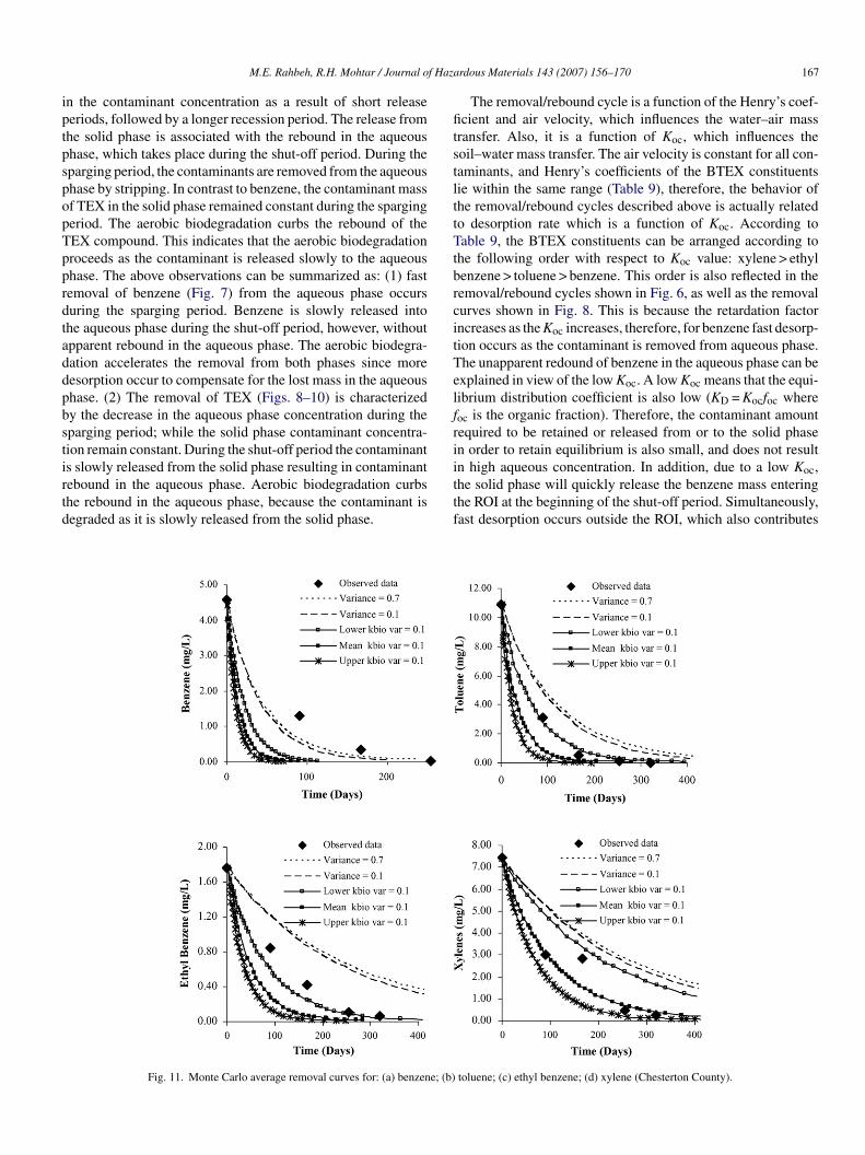
f Haza

iptpspopTpprdtaddpbstirtd

fitstlttTtbrcitTelfri


n the contaminant concentration as a result of short releaseeriods, followed by a longer recession period. The release fromhe solid phase is associated with the rebound in the aqueoushase, which takes place during the shut-off period. During theparging period, the contaminants are removed from the aqueoushase by stripping. In contrast to benzene, the contaminant massf TEX in the solid phase remained constant during the spargingeriod. The aerobic biodegradation curbs the rebound of theEX compound. This indicates that the aerobic biodegradationroceeds as the contaminant is released slowly to the aqueoushase. The above observations can be summarized as: (1) fastemoval of benzene (Fig. 7) from the aqueous phase occursuring the sparging period. Benzene is slowly released intohe aqueous phase during the shut-off period, however, withoutpparent rebound in the aqueous phase. The aerobic biodegra-ation accelerates the removal from both phases since moreesorption occur to compensate for the lost mass in the aqueoushase. (2) The removal of TEX (Figs. 8–10) is characterizedy the decrease in the aqueous phase concentration during theparging period; while the solid phase contaminant concentra-ion remain constant. During the shut-off period the contaminant
s slowly released from the solid phase resulting in contaminantebound in the aqueous phase. Aerobic biodegradation curbshe rebound in the aqueous phase, because the contaminant isegraded as it is slowly released from the solid phase.
ittf

Fig. 11. Monte Carlo average removal curves for: (a) benzene; (b)

rdous Materials 143 (2007) 156–170 167

The removal/rebound cycle is a function of the Henry’s coef-cient and air velocity, which influences the water–air mass

ransfer. Also, it is a function of Koc, which influences theoil–water mass transfer. The air velocity is constant for all con-aminants, and Henry’s coefficients of the BTEX constituentsie within the same range (Table 9), therefore, the behavior ofhe removal/rebound cycles described above is actually relatedo desorption rate which is a function of Koc. According toable 9, the BTEX constituents can be arranged according to

he following order with respect to Koc value: xylene > ethylenzene > toluene > benzene. This order is also reflected in theemoval/rebound cycles shown in Fig. 6, as well as the removalurves shown in Fig. 8. This is because the retardation factorncreases as the Koc increases, therefore, for benzene fast desorp-ion occurs as the contaminant is removed from aqueous phase.he unapparent redound of benzene in the aqueous phase can bexplained in view of the low Koc. A low Koc means that the equi-ibrium distribution coefficient is also low (KD = Kocfoc whereoc is the organic fraction). Therefore, the contaminant amountequired to be retained or released from or to the solid phasen order to retain equilibrium is also small, and does not result
n high aqueous concentration. In addition, due to a low Koc,he solid phase will quickly release the benzene mass enteringhe ROI at the beginning of the shut-off period. Simultaneously,ast desorption occurs outside the ROI, which also contributes
toluene; (c) ethyl benzene; (d) xylene (Chesterton County).

1 f Hazardous Materials 143 (2007) 156–170

ts

4

iditvitbaesaflrthCsmTbatta

Table 10The effect of the variance on the probability of the average contaminant removal

Variance Probability of the average contaminant removal (%)

0.1 8800

rCrflorvpdhCirThptiw


o nearly constant benzene aqueous concentration during thehut-off period.

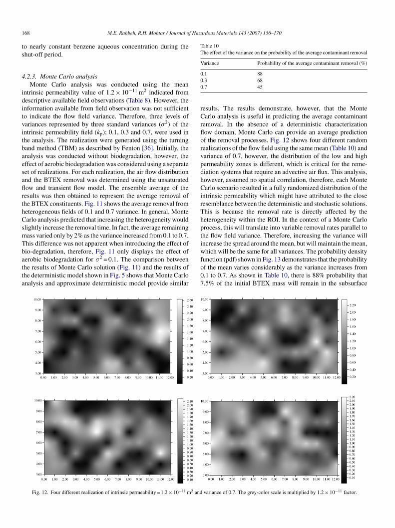
.2.3. Monte Carlo analysisMonte Carlo analysis was conducted using the mean

ntrinsic permeability value of 1.2 × 10−11 m2 indicated fromescriptive available field observations (Table 8). However, thenformation available from field observation was not sufficiento indicate the flow field variance. Therefore, three levels ofariances represented by three standard variances (σ2) of thentrinsic permeability field (kp); 0.1, 0.3 and 0.7, were used inhe analysis. The realization were generated using the turningand method (TBM) as described by Fenton [36]. Initially, thenalysis was conducted without biodegradation, however, theffect of aerobic biodegradation was considered using a separateet of realizations. For each realization, the air flow distributionnd the BTEX removal was determined using the unsaturatedow and transient flow model. The ensemble average of theesults was then obtained to represent the average removal ofhe BTEX constituents. Fig. 11 shows the average removal frometerogeneous fields of 0.1 and 0.7 variance. In general, Montearlo analysis predicted that increasing the heterogeneity would

lightly increase the removal time. In fact, the average remainingass varied only by 2% as the variance increased from 0.1 to 0.7.his difference was not apparent when introducing the effect ofio-degradation, therefore, Fig. 11 only displays the effect of
erobic biodegradation for σ2 = 0.1. The comparison betweenhe results of Monte Carlo solution (Fig. 11) and the results ofhe deterministic model shown in Fig. 5 shows that Monte Carlonalysis and approximate deterministic model provide similar
fo07

Fig. 12. Four different realization of intrinsic permeability = 1.2 × 10−11 m2 and

.3 68

.7 45

esults. The results demonstrate, however, that the Montearlo analysis is useful in predicting the average contaminant

emoval. In the absence of a deterministic characterizationow domain, Monte Carlo can provide an average predictionf the removal processes. Fig. 12 shows four different randomealizations of the flow field using the same mean (Table 10) andariance of 0.7, however, the distribution of the low and highermeability zones is different, which is critical for the reme-iation systems that require an advective air flux. This analysis,owever, assumed no spatial correlation, therefore, each Montearlo scenario resulted in a fully randomized distribution of the

ntrinsic permeability which might have attributed to the closeesemblance between the deterministic and stochastic solutions.his is because the removal rate is directly affected by theeterogeneity within the ROI. In the context of a Monte Carlorocess, this will translate into variable removal rates parallel tohe flow field variance. Therefore, increasing the variance willncrease the spread around the mean, but will maintain the mean,hich will be the same for all variances. The probability density

unction (pdf) shown in Fig. 13 demonstrates that the probabilityf the mean varies considerably as the variance increases from.1 to 0.7. As shown in Table 10, there is 88% probability that.5% of the initial BTEX mass will remain in the subsurface

variance of 0.7. The grey-color scale is multiplied by 1.2 × 10−11 factor.


FB

aar

5

tbTCitnmeidcobttiwes

st[asssa

cBtsup

ovr

rtAiaioevCato

A

Fsc6Sc

R

[

ig. 13. The probability density function of the percentage of the remainingTEX contaminant.

t the end of the sparging period. This probability decreases tobout 68% and 45% as the variance increases to 0.3 and 0.7,espectively.

. Conclusions

In this paper, we applied an unsaturated air flow and mul-iphase contaminant transport model to assess the influence ofiodegradation and pulsed sparging on the BTEX removal rate.wo air sparging operations previously conducted in Porter andhesterton counties of Indiana were simulated. Due to the lim-

ted data availability, a symmetrical subset of two well was usedo represent the entire field. For both case studies, the contami-ant concentration in the ground water was obtained from localonitoring wells within or beside the site in question. An initial

quilibrium was assumed between phases in order to obtain thenitial contaminant concentration in various phases. All inputata, with the exception of first-order aerobic biodegradationoefficients were determined independently from available fieldbservations and the literature. As for the first-order aerobiciodegradation, a range of applicable values was selected fromhe literature. Uncertainty analysis was then conducted to assesshe effect of aerobic biodegradation on the BTEX removal dur-ng air sparging. To enable the pulsed sparging simulation, itas assumed that the contaminant redistributed uniformly at the

nd of each operation period. The simulated results of both casetudies were consistent with the observed data.

The simulated contaminant removal of the Porter County casetudy confirmed previous field observation that only a small frac-ion the contaminant was removed by stripping and volatilization31], while the rest of contaminant reduction was attributed toerobic degradation. Seepage is also an important process thathould not be ignored; in this model, seepage was taken as aink term because of the limitation imposed by the steady stateolution of the air flow distribution which assumes a stagnantqueous phase.

The results of the Chesterton County case study showed closeomparison between the simulated and observed results of theTEX concentration in the aqueous phase, which indicated that

he model was able to adequately predict removal of BTEX con-tituents using pulsed air sparging. This also suggests that theniform redistribution of the contaminant after each spargingeriod is a valid assumption. The removal and rebound cycles

[

rdous Materials 143 (2007) 156–170 169

bserved as a result of the AS operation showed that the Kocalues play a measurable role in controlling the contaminantemoval from the subsurface.

The resemblance between the simulated and the observedesults cannot serve as verification for the model because ofhe assumptions used to evaluate some of the input parameters.ltering any of these assumptions will change the numer-

cal results significantly, although they were predeterminednd carefully rationalized. Therefore, detailed monitoring andnvestigation of the effect of the natural attenuation processesn contaminant removal are essential in order to study theffectiveness of air sparging as remediation technique, and toerify perspective numerical models. The analysis of Porter andhesterton case studies revealed the importance of the model tossess the contaminant mass removal processes during advec-ive air flux, which can be helpful in the decision and operationf AS/SVE systems in practice.

cknowledgements

This research was funded by grant form Purdue Researchoundation under grant number PRF 690-1146-3039, andupport from Environmental Quality Lab, Department of agri-ultural and Biological Engineering under award number903039. Special thanks to Mr. Steve Stanford of IES Inc.chererville, Indiana, for providing field remediation reports andonsultation during this work.

eferences

[1] EPA, Soil Screening Guidance: User’s Guide, EPA, Washington, DC, 1996.[2] L.A. Abriola, G.F. Pinder, A multiphase approach to the modeling of porous

media contamination by organic compounds. 1: equation development,Water Resour. Res. 21 (1) (1985) 11–18.

[3] M.Y. Corapcioglu, A.L. Baehr, A compositional multiphase model forgroundwater contamination by petroleum products. 1: theoretical consid-erations, Water Resour. Res. 23 (1) (1987) 191–200.

[4] B.E. Sleep, J.F. Sykes, Compositional simulation of groundwater contam-ination by organic compounds. 1: model development and verification,Water Resour. Res. 29 (6) (1993) 1697–1708.

[5] B.E. Sleep, J.F. Sykes, Modeling the transport of volatile organics in vari-ably saturated media, Water Resour. Res. 25 (1) (1989) 81–92.

[6] M.L. Brusseau, Transport of organic chemicals by gas advection instructured or heterogeneous porous media: development of a model andapplication to columns experiments, Water Resour. Res. 27 (12) (1991)3189–3199.

[7] J.E. Armstrong, E.O. Frind, R.D. McClellan, Nonequilibrium mass transferbetween the vapor, aqueous, and solid phases in unsaturated soils duringvapor extraction, Water Resour. Res. 30 (2) (1994) 355–368.

[8] A.J.A. Unger, Sudicky, P.A. Forsyth, Mechanisms controlling vacuumextraction coupled with air sparging for remediation of heterogeneous for-mations contaminated by dense nonaqueous phase liquids, Water Resour.Res. 31 (8) (1995) 1913–1925.

[9] J.E. McCray, R.W. Falta, Numerical simulations of air sparging for reme-diation of NAPL contamination, Ground Water 35 (1) (1997) 99–110.

10] K.M. Rathfelder, J.R. Lang, L.M. Abriola, A numerical model (MISER) forthe simulation of coupled physical, chemical and biological processes in
soil vapor extraction and bioventing systems, J. Contam. Hydrol. 43 (2000)239–270.
11] L.A. Abriola, G.F. Pinder, A multiphase approach to the modeling of porousmedia contamination by organic compounds. 2: numerical simulation,Water Resour. Res. 21 (1) (1985) 19–26.

1 f Haza

[

[

[

[

[

[

[

[

[

[

[

[

[

[

[

[

[

[

[

[

[

[

[

217–236.


12] B.E. Sleep, J.F. Sykes, Compositional simulation of groundwater contam-ination by organic compounds. 2: model application, Water Resour. Res.29 (6) (1993) 1709–1718.

13] A.L. Baehr, M.Y. Corapcioglu, A compositional multiphase model forgroundwater contamination by petroleum products. 2: numerical solution,Water Resour. Res. 23 (1) (1987) 201–213.

14] A.J. Radideau, J.M. Blayden, C. Ganguly, Field performance of air-sparging system for removing TCE from groundwater, Environ. Sci.Technol. 33 (1) (1999) 157–162.

15] M.L. Benner, R.H. Mohtar, L.S. Lee, Factors affecting air sparging remedi-ation systems using field data and numerical simulations, J. Hazard. Mater.B 95 (2002) 305–329.

16] P.D. Lundegrad, D. LaBrecque, Air sparging in a sandy aquifer (Florence,Oregon, U.S.A.): actual and apparent radius of influence, J. Cont. Hydrol.19 (1995) 1–27.

17] D.J. McKay, L.J. Acomb, Neutron moisture probe measurements of fluiddisplacement during in-situ air sparging, Ground Water Monit. Remediat.(1996) 86–94.

18] K.R. Reddy, J.A. Adams, Effect of ground water flow on remediation ofdissolved-phase VOC contamination using air sparging, J. Hazard. Mater.72 (2000) 147–165.

19] J.W. Massmann, Applying ground water flow models in vapor extractionsystem design, J. Environ. Eng. 115 (1) (1989) 129–149.

20] C.S. Sawyer, M. Kamakoti, Optimal flow rates and well locations for soilvapor extraction and design, J. Contam. Hydrol. 32 (1998) 63–76.

21] R.H. Mohtar, L.J. Segerlind, R.B. Wallace, Finite element analysis for airsparging in porous media, Fluid/Particle Sep. J. 9 (3) (1996) 225–239.

22] J.L. Wilson, S.H. Conard, E. Hagan, W.R. Mason, W. Peplinski, E. Hagan,Laboratory investigation of residual organics, Report CR-813571, U.S.Environmental Protection Agency, Ada, OK, 1990.

23] M. Hassanizadeh, W.G. Gray, General conservation equations for multi-phase systems: 1: averaging procedure, Adv. Water Resour. 2 (1979)131–144.

24] C.W. Fetter, Contaminant Hydrogeology, Prentice Hall, Inc., New Jersey,1999.

[

[


25] K. Chao, S.K. Ong, A. Protopapas, Water-to-air mass transfer of VOCs:laboratory-scale air sparging system, J. Environ. Eng. 124 (11) (1998)1054–1060.

26] M.D. Wilkins, L.M. Abriola, K.D. Pennell, An experimental investiga-tion of rate-limited nonaqueous phase liquid volatilization in unsaturatedporous media: steady state mass transfer, Water Resour. Res. 31 (9) (1995)2159–2172.

27] S.E. Powers, L.M. Abriola, W.J. Weber, An experimental investigationof nonaqueous phase liquid dissolution in saturated subsurface systems:steady state mass transfer rates, Water Resour. Res. 28 (10) (1992)2691–2705.

28] M.L. Brusseau, P.S.C. Rao, The influence of sorbate–organic matterinteractions on sorption nonequilibrium, Chemosphere 18 (9/10) (1989)1691–1706.

29] A.T. Corey, Mechanics of Immiscible Fluids in Porous Media, WaterResources Publications, Littleton, CO, 1986.

30] M.C. Marley, D.J. Hazebrouck, M.T. Walsh, The application of in-situ airsparging as an innovative soils and groundwater remediation technology,Ground Water Monit. Remediat. 12 (2) (1992) 137–144.

31] S.M. Standford, Physical and biological effects of in situ air sparging ofgroundwater contaminated with organic chemicals, M.Sc. Thesis, PurdueUniversity, West Lafayette, IN, 1998.

32] S.S. Suthersan, Remediation Engineering, Lewis Publishers, Boca Raton,FL, 1997.

33] S.M. Stanford, S. Manti, SVE and Air Sparging Pilot Study (Pilot Plan),ELF Site 9404534 Remediation, Town of Chesterton, Integrated Environ-mental Solution Inc., Schereville, Indiana, 1996.

34] M.L. Benner, S.M. Stanford, L.S. Lee, R.H. Mohtar, Field and numericalanalysis of in situ air sparging: a case study, J. Hazard. Mater. 27 (2000)

35] R.P. Schwarzenbach, P.M. Gschwend, D.M. Imboden, Environmentalorganic chemistry, John Wiley and Sons, Inc., 1993.

36] G.A. Fenton. Simulation and analysis of random fields, Ph.D. Thesis,Princeton University, Princeton, New Jersey, 1990.

application of multiphase transport models to field remediation by air sparging and soil vapor...

Documents