USING GROUNDWATER MODELING AND CONTAMINANT TRANSPORT

PROGRAMS SUCH AS QUICK DOMENICO AND GROUNDWATER VISTAS TO

FURTHER OUR UNDERSTANDING OF REMEDIATION SITES

ABSTRACT

Groundwater remediation can be expensive and time-consuming. Groundwater modeling software and statistical spreadsheet models can save money and time through simulating groundwater flow and optimizing remediation strategies. Models such as the Quick Domenico Fate-and-Transport model plot contaminant transport in one dimension, whereas Groundwater Vistas allows the user to model in three dimensions with known values, allowing a deeper understanding of groundwater flow and contaminant plume movement. This study will review the strengths and limitations of both modeling programs using data from publically available case studies in order to better understand their contributions to remediation strategies. A better knowledge of the groundwater system can reduce remediation costs in the long term, however this must be balanced with the upfront cost of data collection and initial model construction.

INTRODUCTION/ LITERATURE REVIEW

It benefits us as scientists to always look for new tools in which to further our

work. This is why I have chosen to do a study on groundwater modeling software and

contaminant transport programs. Three case studies were chosen with publicly

available data in which to examine and review several modeling programs. The main

focus is to determine how these programs can best further one’s knowledge of a

particular site and whether a one dimensional flow model is sufficient for designing a

remediation strategy or whether it would be more beneficial to apply a three dimensional

model to better understand groundwater flow in a more realistic setting. The two

| 2

programs chosen to review serve their own specific purpose, but also have limitations.

It is the goal of this study to explore these limitations to determine which program is best

in each unique case.

Groundwater remediation is typically very expensive and time-consuming,

therefore companies that are tasked with cleaning up a particular site can use

simulations to predict groundwater flow and models to design optimal remediation

systems for their particular site. (Fan, 2014) Many peer reviewed journals that focus on

groundwater modeling and remediation are cost-centric. This is to be expected as cost

is a determining factor on every site project. The type and complexity of a remediation

system may be determined based on available funds, therefore effective data analysis

is crucial in determining where funds are best spent. In many cases, “flow and transport

models are typically used to process site-specific hydrogeological data. (Compernolle,

2013) Site managers who prefer to use pump and treat techniques can apply models in

which flow patterns are exhibited based on the design of each pump and treat strategy.

Through modeling, site managers can determine which strategy is most cost effective to

implement.

The main goal of any remediation project is to contain the contaminant plume. A

successful remediation shows a decreasing contaminant mass or concentration over

time. This can be done by studying plume stability over time. Ricker (2008) proposes

that this can be done by multiple means. Graphical methods such as isopleth maps,

concentration v. time plots, and concentration v. distance can be used, however in the

case of isopleth maps, human bias can change results. Ricker (2008) suggests that a

statistical method would be more effective. While statistical methods include regression

| 3

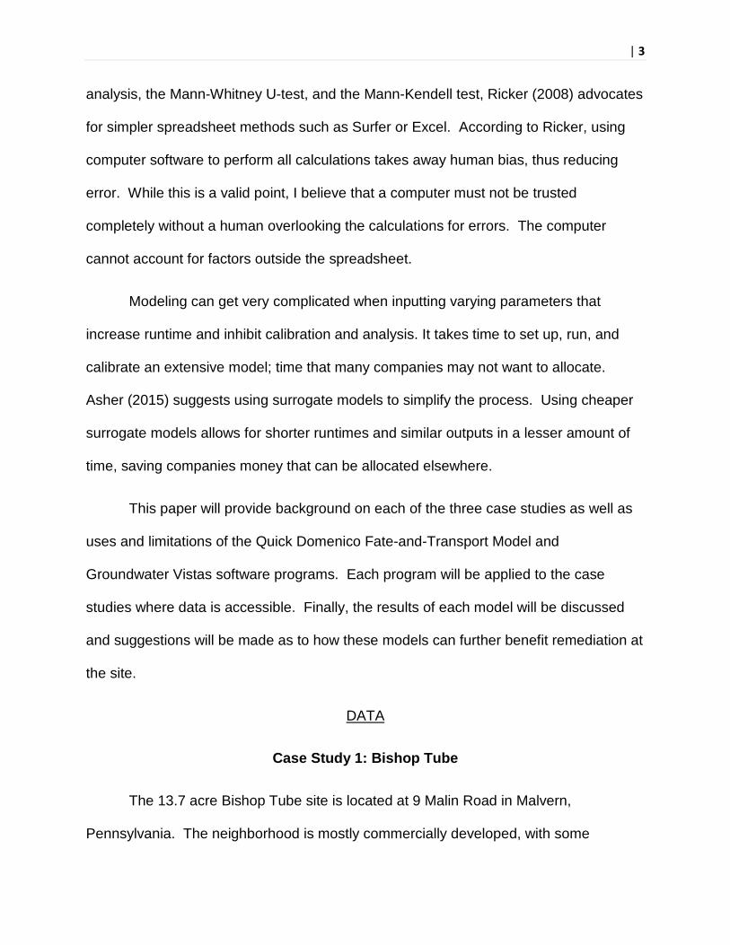
analysis, the Mann-Whitney U-test, and the Mann-Kendell test, Ricker (2008) advocates

for simpler spreadsheet methods such as Surfer or Excel. According to Ricker, using

computer software to perform all calculations takes away human bias, thus reducing

error. While this is a valid point, I believe that a computer must not be trusted

completely without a human overlooking the calculations for errors. The computer

cannot account for factors outside the spreadsheet.

Modeling can get very complicated when inputting varying parameters that

increase runtime and inhibit calibration and analysis. It takes time to set up, run, and

calibrate an extensive model; time that many companies may not want to allocate.

Asher (2015) suggests using surrogate models to simplify the process. Using cheaper

surrogate models allows for shorter runtimes and similar outputs in a lesser amount of

time, saving companies money that can be allocated elsewhere.

This paper will provide background on each of the three case studies as well as

uses and limitations of the Quick Domenico Fate-and-Transport Model and

Groundwater Vistas software programs. Each program will be applied to the case

studies where data is accessible. Finally, the results of each model will be discussed

and suggestions will be made as to how these models can further benefit remediation at

the site.

DATA

Case Study 1: Bishop Tube

The 13.7 acre Bishop Tube site is located at 9 Malin Road in Malvern,

Pennsylvania. The neighborhood is mostly commercially developed, with some

| 4

residential area on the north and east sides of the site. It is noteworthy to mention that

across Malin Road from the Bishop Tube site sits a bulk fuel oil terminal owned by the

Sunoco Corporation. Little Valley creek is the nearest water source to the site, with its

headwaters beginning just south of the site and running northeast. PCE

(Perchloroethylene) and TCE (Trichloroethylene) have both been detected in samples

taken from the creek between a quarter mile and one mile north and northeast of the

site, indicating that the creek has indeed been impacted by the contaminant plume.

However, water from the creek is not used for human consumption as residents in the

area are supplied by city water.

The Bishop Tube site was the home to manufacturing of seamless metal tubes

and other stainless steel specialty items. The two buildings used for manufacturing

were constructed between 1950 and 1959, with manufacturing conducted under the

J.Bishop and Company. The company applied the use of solvents, coolants, oils,

lubricants, acids, alloys, and compounds in order to produce their products. As a result,

the site is now home to a large chlorinated solvent plume that is migrating northeast of

the site. There are three known source areas on the site that are the cause of three

highly concentrated areas. These include two plant degreaser areas and a former drum

storage area. Contaminants found at the site include TCE, its daughter products,

mishandled oils, hydrofluoric acid, and nitric acid.

The site sits atop the Conestoga Formation which is comprised of mostly

limestone and dolomite. Just south of the site lies the Octoraro Formation which is

comprised mostly of schist, chlorite, albite, phyllite, and some gneiss. The extent of

these formations can be seen the two satellite images below, courtesy of Google Earth

| 5

and USGS. The aquifer beneath this site has been characterized as a fractured

bedrock system.

Figure 1: This Google Earth image of the Bishop Tube site (place marked above) sits

atop the Conestoga Formation, shown by a Geologic Map overlay, provided by USGS.

| 6

Figure 2: This Google Earth image of the Bishop Tube site (place marked above) is

located just north of the Octorara Formation, shown by a Geologic Map overlay,

provided by USGS.

The site has been subject to environmental investigations since 1972. The

PADEP is currently remediating the area using multiple techniques including air

sparging and soil vapor extraction to address groundwater and soil contamination. The

site may be up for redevelopment in the near future as developers are looking into

building townhomes where the plant currently stands.

| 7

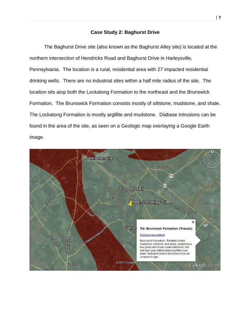
Case Study 2: Baghurst Drive

The Baghurst Drive site (also known as the Baghurst Alley site) is located at the

northern intersection of Hendricks Road and Baghurst Drive in Harleysville,

Pennsylvania. The location is a rural, residential area with 27 impacted residential

drinking wells. There are no industrial sites within a half mile radius of the site. The

location sits atop both the Lockatong Formation to the northeast and the Brunswick

Formation. The Brunswick Formation consists mostly of siltstone, mudstone, and shale.

The Lockatong Formation is mostly argillite and mudstone. Diabase intrusions can be

found in the area of the site, as seen on a Geologic map overlaying a Google Earth

image.

| 8

Figure 3: This Google Earth image of the Baghurst Drive site (place marked above) sits

atop the Brunswick Formation, shown by a Geologic Map overlay, provided by USGS.

Figure 4: This Google Earth image of the Baghurst Drive site (place marked above)

shows the nearby Diabase intrusion, shown by a Geologic Map overlay, provided by

USGS. It is believed that some of this diabase intrudes below the site.

The Brunswick and Lockatong Formations both dip to the southwest. This

means that the Brunswick is thicker at the southwest and pinches off in the northeast.

At the site, the two formations interfinger, placing a thick wedge of the Lockatong

Formation between two layers of the Brunswick Formation. The layering of the

Lockatong Formation and the Brunswick Formation forms a series of confining and

| 9

water-bearing units that together form a leaky, multi-aquifer system. The Lockatong is

considered the confining or semi-confining unit, while the Brunswick Formation is

considered the water-bearing unit. Groundwater generally flows to the southwest at this

site as it mimics topography. The majority of wells in the neighborhood are within the

Brunswick Formation at depths of around 150 to 300 feet bgs (below ground surface)

and are cased to about 20-40 feet bgs. There are some monitoring and drinking wells

screened in the Lockatong Formation.

This site has no identified source of contamination, but contains a groundwater

plume in the general vicinity. The plume measures about 2,500 feet in length and 750

feet wide. Contaminants found include 1,1,1-TCA, 1,1-DCE, TCE, 1,4-dioxane, and

vinyl chloride. This was first brought to the attention of the Montgomery County Health

Department in 1999 when a homeowner submitted a water sample to receive a permit

for a well. Multiple VOCs (volatile organic compounds) were found to be above US EPA

drinking water standards. The PADEP was notified, and bottled water and carbon

filtration systems were provided to the 27 residences impacted.

In 2001, and investigation was conducted at a farm on Hendricks Road by Foster

Wheeler Environmental Corporation. Here they found the highest VOC concentrations.

They also found that the plume had migrated about 800 feet downgradient. It was

rumored that waste had been dumped on the farm, of which the farm owners deny any

dumping had occurred. As a result, there was not enough evidence to identify the farm

as the primary source of contamination.

In 2007 and 2013, the PADEP attempted to find an alternate source of

groundwater for the affected residents, but instead found potential wells to contain

| 10

elevated levels of arsenic and lead. This is believed to be naturally occurring due to

diabase intrusions into the bedrock below.

Case Study 3: Valmont TCE

The Valmont TCE Superfund site is located in West Hazleton, Pennsylvania in a

neighborhood of mixed residential and commercial properties. This site was the home

of a manufacturing facility and has a history of using chlorinated solvents. The plant

that is the known source area is a former upholstery manufacturing plant owned by

Chromatex, Inc. Although Chromatex was the owner and operator, the property was

first leased by the Valmont group, lending its name to this project. The plant was

operational from 1979 to 1993 and is now leased to Karchner Logistics, Inc. who uses

the building as a warehouse for non-hazardous material storage. Chromatex used

fluorocarbon stain repellants containing TCE that lead to the contamination of the site

with VOCs (volatile organic compounds) and a plume that measures about 2,000 feet

long by 400 feet wide by 110 feet deep. Contaminants of concern at this location

include TCE, cis-1,2-DCE, 1,1,1-TCA, and Vinyl chloride.

Contamination was first noted on the site in October 1987 by the now PADEP

(formerly the Pennsylvania Department of Environmental Resources) while sampling at

a neighboring facility for xylene. Once the PADEP found elevated levels of VOCs in

residential drinking wells, they called in the EPA (Environmental Protection Agency) for

help. The highest TCE concentrations found in residential wells was 1.4 ppm (parts per

million). They also tested a well on the property by the plant and found TCE

| 11

concentrations of 2.2 ppm. Bottled water was suppled and eventually city water was

piped to neighboring residents to supply clean water. In 1988, Chromatex installed 12

monitoring wells on the property and found that one well had TCE concentrations of 17

ppm. Other wells also have elevated levels of TCE. The Valmont TCE site was added

to the National Priorities List in September 2001.

The site itself is relatively flat and slopes to the north. It is surrounded by rolling

hills and mountainous terrain. The plant area and surrounding neighborhood covers

about 25 acres. The nearest surface water body is Black Creek, about 1,200 feet north

of the plant. A tributary of Stony Creek runs south of the plant. The site is located in

the Appalachian Mountains within the Valley and Ridge Province. At this particular

location, average depth to bedrock is about 14 feet bgs (below ground surface) and sits

atop the Pottsville Formation, which is composed of mostly conglomerates and

sandstones. Below the Pottsville Formation lies the Maunch Chunk Formation, found at

a depth of less than 300 feet bgs, which is comprised of siltstone, claystone, and

sandstone. A description of the Pottsville formation can be found on the image below,

courtesy of Google Earth and USGS. There is a groundwater divide that runs across

the plant itself, causing contamination to flow away from the plant in two different

directions.

| 12

Figure 5: This Google Earth image of the Valmont site (place marked above) sits atop

the Pottsville Formation, shown by a Geologic Map overlay, provided by USGS.

QUICK DOMENICO

The Quick Domenico Groundwater Fate-and-Transport Model is used by the

Pennsylvania Department of Environmental Protection to solve the groundwater

transport equation for dissolved contaminant plumes. The Excel spreadsheet allows

you to input data, including dispersivity, source concentration, decay constant, hydraulic

conductivity, effective porosity, bulk density and other variables relating to the site. The

result is a two-dimension grid of concentration over distance. This model has many

| 13

applications. It can be used to estimate the length or area of a contaminate plume and

whether it will spread and migrate in the future.

The Quick Domenico model makes some assumptions, as does every model. It

assumes that the aquifer is homogenous and isotropic. It also assumes that the

groundwater flow is homogenous as well as unidirectional and in steady state. The last

assumption is that the contaminant source remains constant in time. Results may not

reflect actual conditions, but it is a model and will most likely not be perfect. The Quick

Domenico model was created for aquifers in porous media, meaning that it cannot be

used for Karst and if modeling fractured bedrock, extra attention must be paid during

calibration. Quick Domenico only simulates first-order decay of contaminants, such as

PAHs (Polycyclic aromatic hydrocarbons), and does not directly account for daughter

products of chlorinated VOCs (volatile organic compounds) without changing certain

parameters. According to the manual, the model should only be used for organic

contaminants that experience natural degradation. Another limitation to the Quick

Domenico model is that it applies to problems that stem from natural attenuation of

contaminants. This model loses its effectiveness with sites that have undergone

remediation. This model also loses its effectiveness when newer sites that have

ethanol in the fuel are involved. Ethanol changes how the other chemicals decay and

move and Quick Domenico simply cannot simulate these conditions. The model’s final

limitation includes NAPLs (non-aqueous phase liquids). Quick Domenico cannot model

the fate and transport of the NAPLS themselves, however it can model the dissolved

plume that originates from the NAPLs.

| 14

GROUNDWATER VISTAS

Groundwater Vistas is a user interface that allows the user to run many different

groundwater modeling programs such as MODFLOW, MODPATH, SEAWAT, and

MT3DS among others. Users can build a complex three-dimensional groundwater flow

model in order to visualize a site and help solve problems associated with said site.

This, combined with the user’s knowledge of hydrogeology, can allow the user to take

phase 1 site data and develop a conceptual site model that will further progress site

remediation and assessment.

Groundwater vistas uses a finite-difference grid, letting you choose the size of

each grid and the amount of boxes in the grid depending on the size and complexity of

your model. You can then input specific boundary conditions and hydraulic properties

of the site.

RESULTS

The Quick Domenico spreadsheet is a useful tool for modeling transport of

PAH’s, but not effective in modeling chlorinated VOCs or NAPLs. The limiting factor

when using this model is the main contaminant at each site. In the case of the three

chosen studies, (chosen at random,) all of my main contaminants happened to be

chlorinated VOCs. For further exploration of this paper, one could search for case

| 15

studies that have PAH’s (such as benzene) as their main contaminants. It is

recommended by the PADEP in the Quick Domenico manual to use Biochlor to model

chlorinated VOCs as it does take daughter products into account. To expand on this

paper one could use Biochlor and compare it to Quick Domenico. For this paper, I

chose to model TCE at the Valmont site to show why the model cannot be used for

chlorinated VOCs. There are plots for both the shallow (Figure 6) and deep (Figure 7)

wells, shown below. Analyzing both plots, you will notice that the concentration of TCE

in the field data drops considerably much earlier than the model predicts. This further

proves that Quick Domenico cannot factor in the production of daughter products

through degradation of chlorinated VOCs.

| 16

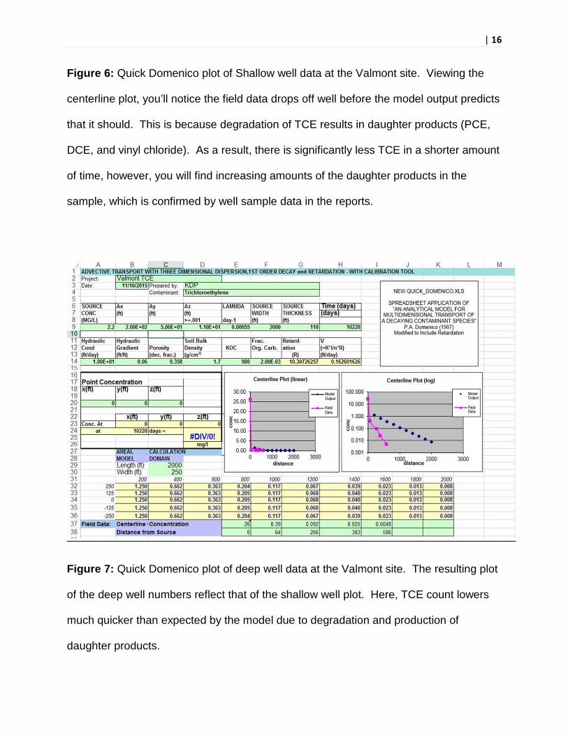
Figure 6: Quick Domenico plot of Shallow well data at the Valmont site. Viewing the

centerline plot, you’ll notice the field data drops off well before the model output predicts

that it should. This is because degradation of TCE results in daughter products (PCE,

DCE, and vinyl chloride). As a result, there is significantly less TCE in a shorter amount

of time, however, you will find increasing amounts of the daughter products in the

sample, which is confirmed by well sample data in the reports.

Figure 7: Quick Domenico plot of deep well data at the Valmont site. The resulting plot

of the deep well numbers reflect that of the shallow well plot. Here, TCE count lowers

much quicker than expected by the model due to degradation and production of

daughter products.

| 17

Figure 8: The plot above shows model output adjusted using Lambda (the decay

constant) to closely resemble field data.

Groundwater Vistas is a complex modeling program that has many uses. It can

be made as simply or as complicated as the user chooses. For contaminant transport,

running MODFLOW, MODPATH and MT3DS is most effective as you can track

particles from various locations around the site or contaminant source to see where they

will migrate over time. In the study basic models were developed of all three case

studies in order to mimic what is occurring at the sites. Groundwater Vistas requires

multiple steps, therefore I will walk through the process for the Baghurst site model

using the next few figures.

| 18

Figure 9: The picture above is the beginnings of a model for the Baghurst Drive study.

The first step includes inputting a base map with topographic contours. The second

step involves creating polygons of different elevations to recreate the contours of the

area.

| 19

Figure 10: (The top elevations have been turned off for the next few steps in order to

better visualize the following elements.) The third step includes placing the Perkiomen

Creek as seen coming in from the left of the model and exiting to the south. The orange

rectangle is the area of initial highest concentrations found at the farm on the corner of

Hendricks Road and Baghurst Drive.

| 20

Figure 11: The next step in creating the model involves inputting wells around the site

where concentrations have been found. All wells shown are in red and are pumping.

| 21

Figure 12: According to my interpretation of the report, the contaminant should be

flowing south along the river, but the model shows it flowing directly into the river as you

can see from above by the blue flow lines created by MODFLOW.

| 22

Figure 13: The report showed diabase intrusions just west of the plume, therefore to

model this, which in turn also models why the flowlines do not run directly towards the

river, a no flow boundary is put in place to simulate a diabase intrusion. It is also

important to note here, there is a ridge where I placed the no flow boundary, most likely

the result of a diabase intrusion, which in this region is resistant to weathering.

| 23

Figure 14: With the Diabase intrusion in place, I ran particles through my model and

they tracked just as I suspected, traveling along the East side of the ridge.

| 24

Figure 15: The last command I ran on this model was MT3DS, which tracks

contaminants from an initial concentration. Keeping in mind that this is just a model, we

could predict that eventually the contaminant will reach the Perkiomen Creek,

depending on a few factors: 1) The diabase intrusion is not infinite and somewhere

along the topography it will retreat below the Lockatong and Brunswick Formation,

allowing groundwater and contaminants to once again reach the creek; and 2) The

source of the contamination is not known, and it is possible that it is further north than

originally expected.

| 25

For the remaining two case studies (Bishop Tube and Valmont), I have chosen to

include just a few aspects of each model as I described the process in great detail using

the first case study (Baghurst Alley).

Figure 16: At the Valmont site, a groundwater divide runs right below the site, but only

effects shallow groundwater movement. To demonstrate this, I placed a no flow

boundary across the site in the top two layers, and then placed particles on the site to

model movement. The particles behaved as I expected; the shallow particles moved

away from the site in both directions, while the deep particles moved deeper

underground and went towards the Black Creek north of the site. This can be seen in

the cross section above.

| 26

Figure 17: To complete the Valmont model, I placed a concentrated contaminant at the

site (as shown as an orange box on the model) and ran MT3DS to see the nature of the

plume. The plume mapped as expected, extended in the Northeast and Southwest

directions away from the groundwater divide. This model also agrees with the model

created in the EPA report.

The Bishop Tube site is quite different in comparison to the other two studies in

this paper. The report focuses mainly on health impacts to nearby areas due to

contamination. Therefore, there are only three wells discussed in the paper that were

found to have elevated contaminant levels. Much of the paper discusses elevated

| 27

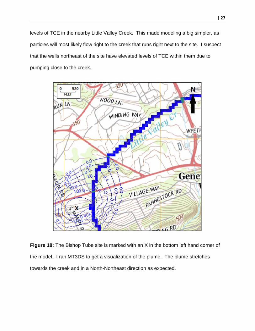
levels of TCE in the nearby Little Valley Creek. This made modeling a big simpler, as

particles will most likely flow right to the creek that runs right next to the site. I suspect

that the wells northeast of the site have elevated levels of TCE within them due to

pumping close to the creek.

Figure 18: The Bishop Tube site is marked with an X in the bottom left hand corner of

the model. I ran MT3DS to get a visualization of the plume. The plume stretches

towards the creek and in a North-Northeast direction as expected.

| 28

CONCLUSIONS

In this paper, I reviewed two groundwater modeling programs, Groundwater

Vistas and the Quick Domenico Fate-and-Transport model. To demonstrate the

strengths and limitations of each program, I applied them to three publically available

case studies. This approach allows an individual to become familiar with each program

through data extraction and trial and error. Each case has a different geology, different

combination of contaminants, and a different history, allowing an individual studying

these programs to apply different techniques each time they use one of these models.

By applying these models to various sites, the user becomes more familiar with the

software and becomes more efficient, so cost of model construction decreases with

time.

The results from this study showed that the Quick Domenico Fate-and-Transport

model is somewhat limited to PAHs and cannot account for NAPLs or degradation of

chlorinated VOCs without adjusting Lambda (the decay constant). The model plots

concentration over distance in one dimension over a specified simulation time. This can

be used to estimate the current length of contaminant plumes as well as predict plume

length over a longer time period. It is also used to assess plume stability. Groundwater

Vistas is a more complex program modeling three dimensional flow based on boundary

conditions and topography. While it allows the user to have a better understanding of

flow at the site, it requires an exponentially larger amount of time to develop. For

example, I was able to run Quick Domenico in less than an hour with successful results,

whereas I have spent close to fifty hours developing my Groundwater Vistas models. If

I were a consultant charging $150 per hour, the client would be spending a large chunk

| 29

of their budget on site modeling alone. However, through Groundwater Vistas, I can

see how contaminants are flowing under the site and around the area more thoroughly

and would be able to provide a more efficient remediation system that could save time

and money in the long term. Also, as one becomes more comfortable using the

software, the time it takes to create a model would decrease, making it more cost

efficient in the long term as well.

With these results, future work may include: 1) applying the Biochlor model to

case studies with chlorinated VOC contaminants and compare those results to those of

Quick Domenico; 2) accessing case studies with PAH’s as main contaminants in order

to apply the Quick Domenico model without having to adjust Lambda; and 3) applying

Groundwater Vistas to more sites to become more efficient with the software.

| 30

REFERENCES

Peer Reviewed Journals

1. Asher, M.J., B.F.W. Croke, A.J. Jakeman, and L.J.M. Peeters (2015), A Review

of surrogate models and their application to groundwater modeling, Water

Resources Research, 51, 5957-5973, doi:10.1002/2015WR016967.

2. Compernolle, T., S. Van Passel, and L. Lebbe (2013), The Value of Groundwater

Modeling to support a Pump and Treat Design, Groundwater Modeling and

Remediation, 33, no.3, 111-118, doi: 10.1111/gwmr.12018.

3. Liu, X., J. Lee, P.K. Kitanidis, J. Parker, and U. Kim (2012), Value of Information

as a Context-specific Measure of Uncertainty in Groundwater Remediation,

Water Resour. Manage., 26, 1513-1535, doi: 10.1007/s11269-011-9970-3.

4. Ricker, J.A (2008), A Practical Method to Evaluate Ground Water contaminant

Plume Stability, Groundwater Modeling and Remediation, 28, no. 4, 85-94.

Case Study Information

1. U.S. Department of Health and Human Services (2008), Health Consultation –

Bishop Tube Site, Agency for Toxic Substances and Disease Registry.

2. Baker, L. (2014), HRS Documentation Record – Baghurst Drive, U.S.

Environmental Protection Agency.

3. U.S. EPA (2011), Record of Decision – Valmont TCE Superfund Site.

| 31

Software Manuals

1. Brown, C.D., P. Trowbridge, S. Sayko, and M. Droese (2014), User’s Manual for

the Quick Domenico Groundwater Fate-and-Transport Model, Pennsylvania

Department of Environmental Protection.

2. Duffield, G.M (2007), Aqtesolv for Windows Version 4.5 User’s Guide,

HydroSOLVE, Inc.

3. Rumbaugh, J.O., and D. B. Rumbaugh (2011), Guide to Using Groundwater

Vistas Version 6, Environmental Simulations, Inc.

Maps/Images/Graphics

1. PA Geologic Map – KML file for Google Earth (USGS)

http://mrdata.usgs.gov/geology/state/state.php?state=PA