application of field theoretical methods to problems in mesoscopic physics
TRANSCRIPT

Application of field theoretical methods to problemsin mesoscopic physics
Inaugural-Dissertation
zur
Erlangung des Doktorgrades
der Mathematisch-Naturwissenschaftlichen Fakultat
der Universitat zu Koln
vorgelegt von
Tobias Micklitz
aus Munchen
2006

Berichterstatter: Prof. Dr. A. Altland
Prof. Dr. A. Rosch
Tag der letzten mundlichen Prufung: 09.02 - 28.02.07

Abstract
The subject of this thesis are three different topics related to quantum interference and dephasing inweakly disordered mesoscopic systems.
The first topic covers the so-called “current echo”, which is a quantum-interference phenomenonpredicted about a decade ago by Thomas et al. on the basis of numerical calculations. Our motivationto study the current echo originates from the fact that a simple physical picture explaining its appearanceso far has been missing. It is shown that all characteristic features of Thomas’ current echo can beexplained resorting to the well known phenomenon of weak localization in disordered systems. In viewof recent technological progress in the creation of voltage pulses on a pico-second time scale, theexperimental verification of the current echo should be feasible. The echo phenomenon may become auseful tool to determine dephasing rates in weakly disordered systems.
The second topic is titled “Dephasing by Kondo impurities”. In this part of the thesis we derivean analytical expression for the dephasing rate of non-interacting electrons propagating in a weaklydisordered environment and scattering from very low concentrations of magnetic impurities. The mo-tivation to study dephasing due to Kondo impurities traces back to a series of experiments performedover the last decade which show an unexpected saturation of the dephasing rate at lowest temperat-ures. The observed saturation clearly deviates from theoretical predictions based on the assumptionthat inelastic scattering due to electron-electron interactions is the dominant mechanism for dephasing.Therefore, it was suggested, that inelastic scattering from low concentrations of magnetic impurit-ies may be responsible for the observed excess of dephasing. So far these speculations could not bequantitatively tested, since the dephasing rate due to diluted magnetic impurities in the experimentallyprobed range of temperature was unknown. Based on our results a quantitative comparison betweentheoretically predicted and experimentally measured dephasing rate was done. This allowed for a criticalexamination of the relevance of low concentrations of magnetic impurities for the observed behaviourof the dephasing rate. Moreover, this part of the thesis analyzes the magnetic field dependence ofthe dephasing rate due to magnetic impurities and generalizes the results for the dephasing rate frommagnetic to arbitrary diluted dynamical impurities.
The third topic of this thesis relates to quantum interference and dephasing in a disordered Lut-tinger liquid. The standard approach to describe interacting one-dimensional systems is the bosoniza-tion method, which, however, becomes very intransparent when in addition disorder comes into play.Therefore, quantum interference phenomena and dephasing in a disordered Luttinger liquid remainedunaddressed for a long time. In this part of the thesis we follow a new road and derive an effectivefield theory for the disordered Luttinger liquid. This model allows to systematically explore interferencephenomena in disordered Luttinger liquids. As an application of the model we discuss for the first timethe persistent current in a weakly disordered Luttinger liquid.
3


Zusammenfassung
Die vorliegende Arbeit beschaftigt sich mit drei verschiedenen Themengebieten, in deren Mittelpunktquantenmechanische Interferenzphanomene und der Verlust von Phasenkoharenz (Dephasierung) inschwach ungeordneten mesoskopischen Systemen stehen.
Im ersten Abschnitt der Arbeit diskutieren wir sogenannte “Stromechos”, ein quantenmechanischesInterferenzphanomen, welches vor einem Jahrzehnt von Thomas et al. aufgrund numerischer Rech-nungen vorhergesagt wurde. Die Motivation, uns mit den Stromechos zu beschaftigen, resultiert ausder Tatsache, dass eine einfache physikalische Erklarung dieses Phanomens fehlte. In der Tat kanngezeigt werden, dass alle in den numerischen Rechnungen gefundenen Eigenschaften des Echos mitderselben Physik erklart werden konnen, welche der schwachen Lokalisierung in ungeordneten Systemenzugrundeliegt. Angesichts des rasanten technischen Fortschrittes in der Erzeugung von Spannungspulsenauf Zeitskalen von Pikosekunden, scheint eine experimentelle Verifizierung des Stromechos realisierbar.Praktische Bedeutung konnen die Stromechos in der Bestimmung von Dephasierungsraten erhalten.
Im zweiten Abschnitt, dem Themengebiet “Depahsing due to Kondo impurities”, berechnen wirdie Dephasierungsrate von Elektronen, die durch ein ungeordnetes System propagieren und an einergeringen Konzentration magnetischer Unreinheiten streuen. Unser Interesse an diesem Problem gehtauf zahlreiche Experimente zuruck, welche im Laufe des letzten Jahrzehnts durchgefuhrt wurden undeine unerwartete Sattigung der Dephasierungsrate bei tiefsten Temperaturen zeigen. Die beobachteteSattigung weicht von theoretischen Vorhersagen ab, welche auf der Annahme basieren, dass die Depha-sierung allein durch Elektron-Elektron-Wechselwirkung verursacht wird. Daher wurde vermutet, dassinelastische Streuung an stark verdunnten magnetischen Verunreinigungen den wesentliche Beitrag zurDephasierung bei tiefen Temperaturen liefert. Diese Vermutung konnte jedoch bisher nicht quantita-tiv uberpruft werden, da die Dephasierungsrate, welche von inelastischer Streuung an magnetischenVerunreinigungen herruhrt, in dem experimentell untersuchten Temperaturbereich nicht bekannt war.Basierend auf unserem Ergebnis konnte nun erstmals die Vermutung, dass geringe Konzentrationen vonmagnetische Unreinheiten verantwortlich fur die experimentell beobachtete Sattigung der Dephasier-ungsrate bei tiefen Temperaturen sind, kritisch uberpruft werden. Weiterhin diskutieren wir in diesemAbschnitt der Arbeit die Magnetfeldabhangigkeit der Dephasierungsrate, und verallgemeinern unsereErgebnisse von magnetischen auf beliebige, verdunnte dynamische Verunreinigungen.
Im dritten Abschnitt der Arbeit diskutieren wir quantenmechanische Interferenz und Dephasier-ung in Luttinger-Flussigkeiten. Eine sehr effiziente Methode zur Beschreibung wechselwirkender, ein-dimensionaler Systeme ist das Bosonisierungs-Verfahren. Kommt jedoch zusatzlich Unordnung insSpiel, wird diese Methode sehr undurchsichtig. Deshalb wurden quantenmechanische Interferenz undDephasierung in ungeordneten Luttinger-Flussigkeiten fur lange Zeit nicht untersucht. In diesem Ab-schnitt der Arbeit leiten wir eine effektive Feldtheorie fur ungeordnete Luttinger-Flussigkeiten ab, welcheeine systematische Untersuchung quantenmechanischer Interferenzphenomane erlaubt. Als Anwendungunseres Models diskutieren wir erstmals Dauerstrome in einer ungeordneten Luttinger Flussigkeit.
5


Contents
1 Current-Echoes in Metals and Semiconductors 111.1 Keldysh σ-model for systems with time-reversal invariance . . . . . . . . . . . . . . . 121.2 Current in linear response to a pulsed electrical field . . . . . . . . . . . . . . . . . . . 161.3 Cooperon in a pulsed electric field . . . . . . . . . . . . . . . . . . . . . . . . . . . . 171.4 Semiclassical analysis of the current-echo . . . . . . . . . . . . . . . . . . . . . . . . 201.5 Current-echo in semiconductors . . . . . . . . . . . . . . . . . . . . . . . . . . . . . . 221.6 Summary and outlook . . . . . . . . . . . . . . . . . . . . . . . . . . . . . . . . . . . 26
2 Dephasing by Kondo Impurities 292.1 Replica NLσM for disordered electron gas containing
diluted magnetic impurities . . . . . . . . . . . . . . . . . . . . . . . . . . . . . . . . 302.2 Dephasing by static magnetic impurities . . . . . . . . . . . . . . . . . . . . . . . . . 352.3 Dephasing due to dynamical magnetic impurities . . . . . . . . . . . . . . . . . . . . 37
2.3.1 Introduction of elastic and inelastic vertices . . . . . . . . . . . . . . . . . . . 372.4 Dephasing-rate measured from the magnetoresistance . . . . . . . . . . . . . . . . . . 39
2.4.1 The dephasing rate measured in WL experiments . . . . . . . . . . . . . . . . 392.4.2 1. Contributions from inelastic vertex . . . . . . . . . . . . . . . . . . . . . . 412.4.3 2. Contributions from mixed diagrams . . . . . . . . . . . . . . . . . . . . . . 452.4.4 3. Contributions from higher-order corrections in nS . . . . . . . . . . . . . . 462.4.5 Interplay: Kondo effect and electron-electron interactions . . . . . . . . . . . . 46
2.5 Summary . . . . . . . . . . . . . . . . . . . . . . . . . . . . . . . . . . . . . . . . . . 462.6 Generalizations . . . . . . . . . . . . . . . . . . . . . . . . . . . . . . . . . . . . . . . 472.7 Dephasing-rate measured from universal conductance
fluctuations and Aharonov-Bohm oscillations . . . . . . . . . . . . . . . . . . . . . . . 492.8 Dephasing-rate measured from the current echo . . . . . . . . . . . . . . . . . . . . . 542.9 Comparison to recent experiments and outlook . . . . . . . . . . . . . . . . . . . . . 54
3 Disordered Luttinger Liquid 593.1 The model . . . . . . . . . . . . . . . . . . . . . . . . . . . . . . . . . . . . . . . . . 603.2 Bosonization of non-interacting electrons in a clean wire: three equivalent approaches . 61
3.2.1 Standard bosonization . . . . . . . . . . . . . . . . . . . . . . . . . . . . . . . 613.2.2 Functional bosonization . . . . . . . . . . . . . . . . . . . . . . . . . . . . . . 623.2.3 σ-Model bosonization . . . . . . . . . . . . . . . . . . . . . . . . . . . . . . . 633.2.4 Higher loop corrections to the Gaussian propagator . . . . . . . . . . . . . . . 713.2.5 Summary of this section and outlook . . . . . . . . . . . . . . . . . . . . . . . 72
3.3 Interacting electrons in a clean wire: Equivalence of the three approaches . . . . . . . 723.3.1 Standard bosonization . . . . . . . . . . . . . . . . . . . . . . . . . . . . . . . 723.3.2 Functional bosonization . . . . . . . . . . . . . . . . . . . . . . . . . . . . . . 733.3.3 σ-model bosonization . . . . . . . . . . . . . . . . . . . . . . . . . . . . . . . 743.3.4 Summary of this section . . . . . . . . . . . . . . . . . . . . . . . . . . . . . 74
3.4 Inelastic scattering rate in a clean Luttinger liquid . . . . . . . . . . . . . . . . . . . . 753.4.1 Screening the Coulomb-interactions . . . . . . . . . . . . . . . . . . . . . . . 763.4.2 The inelastic scattering rate . . . . . . . . . . . . . . . . . . . . . . . . . . . 763.4.3 Summary of this section . . . . . . . . . . . . . . . . . . . . . . . . . . . . . 78
7

8
3.5 Electrons in a disordered one-dimensional system . . . . . . . . . . . . . . . . . . . . 783.5.1 Localization in a disordered 1d system . . . . . . . . . . . . . . . . . . . . . . 793.5.2 Drude conductivity and weak localization in a disordered 1d system . . . . . . 803.5.3 Summary of this section . . . . . . . . . . . . . . . . . . . . . . . . . . . . . 81
3.6 Interacting electrons in a disordered 1d system . . . . . . . . . . . . . . . . . . . . . . 823.6.1 RPA screening in a disordered system . . . . . . . . . . . . . . . . . . . . . . 833.6.2 “Renormalization” of disorder by electron-electron interactions . . . . . . . . . 843.6.3 Summary of this section and outlook . . . . . . . . . . . . . . . . . . . . . . . 86
3.7 An Application: Persistent current in a Luttinger liquid . . . . . . . . . . . . . . . . . 863.7.1 Persistent current in a clean Luttinger liquid . . . . . . . . . . . . . . . . . . . 863.7.2 Persistent current in a weakly disordered Luttinger liquid . . . . . . . . . . . . 903.7.3 Summary of this section . . . . . . . . . . . . . . . . . . . . . . . . . . . . . 98
3.8 Summary and outlook . . . . . . . . . . . . . . . . . . . . . . . . . . . . . . . . . . . 98
A Appendix (Dephasing by Kondo impurities) 101A.1 Gradient expansion . . . . . . . . . . . . . . . . . . . . . . . . . . . . . . . . . . . . 101A.2 Spin-singlet and spin-triplet channels . . . . . . . . . . . . . . . . . . . . . . . . . . . 103
A.2.1 Spin-singlet channels . . . . . . . . . . . . . . . . . . . . . . . . . . . . . . . 103A.2.2 Spin-triplet channels . . . . . . . . . . . . . . . . . . . . . . . . . . . . . . . . 104
A.3 Response kernels in Gaussian approximation . . . . . . . . . . . . . . . . . . . . . . . 106A.3.1 Response kernel for weak localization experiment . . . . . . . . . . . . . . . . 106A.3.2 Response kernel for Aharonov-Bohm oscillations . . . . . . . . . . . . . . . . . 107
A.4 Some details . . . . . . . . . . . . . . . . . . . . . . . . . . . . . . . . . . . . . . . . 109A.5 Some more details . . . . . . . . . . . . . . . . . . . . . . . . . . . . . . . . . . . . . 110A.6 Renormalized perturbation theory for the
Anderson model . . . . . . . . . . . . . . . . . . . . . . . . . . . . . . . . . . . . . . 110A.7 Fluctuations of the Kondo-temperature . . . . . . . . . . . . . . . . . . . . . . . . . . 111A.8 Limits of applicability: Cross-over temperatures for the dephasing-rate . . . . . . . . . 112
A.8.1 Evaluation of the diagrams . . . . . . . . . . . . . . . . . . . . . . . . . . . . 114A.9 Analytical continuation . . . . . . . . . . . . . . . . . . . . . . . . . . . . . . . . . . 114
A.9.1 Self-energy corrections ∆σ1 . . . . . . . . . . . . . . . . . . . . . . . . . . . . 114A.9.2 Vertex corrections ∆σ2 . . . . . . . . . . . . . . . . . . . . . . . . . . . . . . 116
A.10 Lehmann representation . . . . . . . . . . . . . . . . . . . . . . . . . . . . . . . . . . 117A.10.1 Self-energy . . . . . . . . . . . . . . . . . . . . . . . . . . . . . . . . . . . . . 117A.10.2 Two-vertex . . . . . . . . . . . . . . . . . . . . . . . . . . . . . . . . . . . . 117A.10.3 Three-vertex . . . . . . . . . . . . . . . . . . . . . . . . . . . . . . . . . . . . 118A.10.4 Four-vertex . . . . . . . . . . . . . . . . . . . . . . . . . . . . . . . . . . . . 119
B Appendix (Disordered Luttinger Liquid) 127B.1 l0-independent contributions from the “ tr ln ”-expansion . . . . . . . . . . . . . . . . 127B.2 Diagrammatic evaluation of the density/density correlation function . . . . . . . . . . 130B.3 Regularization of the propagator . . . . . . . . . . . . . . . . . . . . . . . . . . . . . 131B.4 Equivalence of Eq.(3.68) and Eq.(3.72) . . . . . . . . . . . . . . . . . . . . . . . . . 132B.5 Equivalence of Eq.(3.72) and Eq.(3.74) . . . . . . . . . . . . . . . . . . . . . . . . . 133B.6 Dephasing rates . . . . . . . . . . . . . . . . . . . . . . . . . . . . . . . . . . . . . . 134B.7 Inclusion of back-scattering disorder . . . . . . . . . . . . . . . . . . . . . . . . . . . 135B.8 Some details . . . . . . . . . . . . . . . . . . . . . . . . . . . . . . . . . . . . . . . . 136
B.8.1 Analytical continuation of Sχ[CfbCbf] . . . . . . . . . . . . . . . . . . . . . . . 136B.8.2 Poisson summation . . . . . . . . . . . . . . . . . . . . . . . . . . . . . . . . 137B.8.3 Performing the y-integral . . . . . . . . . . . . . . . . . . . . . . . . . . . . . 137B.8.4 Coulomb field propagator . . . . . . . . . . . . . . . . . . . . . . . . . . . . . 138

Introduction
The quantum mechanical wave-nature of matter not only appears on microscopic scales, but also canbe studied in systems with macroscopic numbers of degree of freedom, as e.g. mesoscopic metalsand semiconductors at low temperatures. The electron’s wave nature manifests itself in its ability tointerfere. Interference effects play an important role in disordered systems: Electrons scatter fromimpurities and form a complicated interference pattern, giving rise, on the one hand, to measurabledeviations from classically expected values of observables, such as the conductivity, and, on the otherhand, leading to new, classically not expected phenomena.
A new “interference-phenomenon”, the so-called current echo, has been predicted by Thomas et
al. about a decade ago. The predictions are based on numerical calculations and a simple physicalinterpretation for the current echo has been missing so far. In the first chapter of this thesis we willdiscuss this phenomenon and suggest an explanation which resorts only to the well-established theoryof weak localization in disordered metals of non-interacting electrons.
In real physical systems the particle are, however, always exposed to interactions, which can beintrinsic (such as electron-electron interactions) or extrinsic due to interactions with an environment(such as dynamical impurities). Inelastic interaction processes lead to the destruction of the electron’s phase coherence and therefore suppress interference phenomena. Phase space arguments lead tothe expectation that dephasing of electrons in a Fermi sea becomes ineffective when the temperatureis lowered. At lowest temperatures the electrons phase coherence should be fully re-established. Ir-ritatingly, however, several experiments performed over the last decade, indicate a saturation of thedephasing rate at lowest temperatures. It was suggested that this excess of dephasing results fromscattering of electrons at extremely low concentrations of magnetic impurities, which are inevitablycontained in the probes. In the second chapter of this thesis we will tackle this problem with the aim toderive an analytical expression for the dephasing rate of electrons interacting with low concentrationsof magnetic impurities.
Interactions not only cause dephasing but may also drastically change the systems properties. Arbit-rary weak electron-electron interactions in one-dimensional systems are known to turn the system intoa non-Fermi liquid state, the so-called Luttinger liquid. The Luttinger liquid is e.g. characterized bypower-laws for the temperature and bias-voltage dependence of the tunneling current, which has beenexperimentally verified e.g. in carbon nanotubes. The standard approach to interacting one-dimensionalsystems is the bosonization method. This method, however, becomes very intransparent when disordercomes into play. Therefore, quantum interference phenomena and dephasing in a Luttinger liquid re-mained unaddresses for a long time. In the third chapter of this thesis we use a different approach toanalyze disordered interacting one-dimensional systems. This approach leads to a field theory which isthe single-channel limit of an “universal” model for disordered interacting systems, known from higherdimensions and which allows for a transparent description of interference phenomena. A practical ap-plication of this model will be the analysis of the persistent current in a disordered single-channel ringof (weakly) interacting electrons.
As indicated in the title we employ field theoretical methods to address the above mentioned prob-lems. More precisely we use the nonlinear σ-model and the closely related diagrammatic perturbationtheory in terms of Greens functions.
9

10

Chapter 1
Current-Echoes in Metals andSemiconductors
Introduction: Based on numerical calculations within the Anderson impurity model of non-interactingelectrons Thomas et al. suggested about a decade ago the existence of current-echoes in disorderedmetals [1]. Experimentally, the generation of such current-echos is highly non-trivial, as it requiresvoltage pulses on time scales shorter than the dephasing time, which is typically of the order or lessthan nano seconds. Indeed, an experimental verification of their existence is so far lacking. Therefore,having in mind the feasibility to optically generate ultra-short current pulses in semiconductors on afemto- to picosecond time scale (by use of coherent control techniques, see e.g. [2, 3, 4]) numericalanalysis of the echo scenario was extended to semiconductors [5, 6]. However, we do not know of anyexperiments probing the echo in semiconductors. Also, in later works the influence of electron-electroninteractions on the echo has been studied [7]. The features characterizing the echo phenomenon inmetals and semiconductors as found by numerical studies can be summarized as follows (the interestedreader can find more details in [1, 5, 6]):
1. Current-echo in metals: A disordered conductor exposed to a short voltage pulse at time t = 0generates a current pulse, which decays within the elastic scattering time. For a system withoutCoulomb interaction and in the absence of other dephasing mechanism, a second voltage pulseat t = t0 leads to the reconstruction of a macroscopic current burst at t = 2t0, opposite insign to the original current pulses. Inclusion of Coulomb interactions (exponentially) reduces theamplitude of the echo.
2. Current-echo in semiconductors: In a two-band semiconductor with correlated disorder (for adefinition of correlated disorder see section 1.5 “Current-Echo in Semiconductors” below) anddifferent masses of the charge carriers in conduction and valence band the application of coherentcontrol schemes at time t = 0 optically generates short inter- and intraband current pulsesdecaying due to elastic scattering from disorder. A second pulse applied at time t = t0 againleads to the appearance of a current-echo. Three main findings characterize the current-echo insemiconductors:
(a) The echo only appears in the model with correlated disorder.
(b) In the case of correlated disorder, the echo even shows up for a simplified excitation sequence,where only the first light-pulse creates inter- and intraband current pulses whereas thesecond pulse is a simple full-gap pulse causing inversion of the band charges. That is, onlyone current pulse — which has to be the first pulse — is necessary to generate the echo.Reversing the order of pulses does not obtain an echo.
(c) Most surprisingly, for different masses, mc < mv, of the charge carriers in the conduction andvalence band, respectively, the intraband current-echo splits into two separate contributions:
a conduction band response at the advanced time tc =(
1 + mc
mv
)
t0 and a delayed response
in the valence band at the retarded time tv =(
1 + mv
mc
)
t0. The interband echo, on the
other hand, always appears at t = 2t0
11
12 CHAPTER 1. CURRENT-ECHOES IN METALS AND SEMICONDUCTORS
Interestingly to us, a simple picture explaining the physics behind the current echo so far has beenmissing. Therefore we found it challenging to look for a microscopic mechanism explaining the diversityof features characterizing the current-echo in metals and semiconductors. An explanation based on theconstructive interference of time-reversed paths is given in the following sections.
Outline: The outline of the rest of the chapter is the following: In order to make this text self-contained we derive in the first section the basic equations (two particle- or “Cooperon”-equation) lyingat the heart of our explanation of the current-echo. These equations can be found in textbooks (e.g.[16]) but we here use a different derivation within the Keldysh σ-model. Rather technical in nature,this section can be skipped as it does not give any new results.
In the second section we repeat [9] that in response to a pulsed electric field, the weak localiza-tion corrections to the conductivity (which can be described in terms of the two particle propagator“Cooperon”) give rise to a negative current, decaying algebraically in time (if perfect phase coherence isassumed). This observation leads us to study in the third section the fate of the Cooperon in the pres-ence of an external electric field, or, more specifically, when a second voltage pulse is applied. Indeed,we show that due to breaking of time-reversal symmetry by the second pulse, the Cooperon becomessuppressed — except for a short moment T = 2t0 when time reversal symmetry is re-established. In thisway we can understand the current-echo as a sudden re-appearance of the weak localization contributionto the current. In the fourth section we re-derive the results of the third section from a semiclassicalapproach, and, finally, in the fifth section employ the semiclassical approach to explain the current-echoin semiconductors.
1.1 Keldysh σ-model for systems with time-reversal invariance
Consider a d-dimensional weakly disordered metal described by the Lagrangian
L[ψψ, φ,A] =
∫
ddxψ(x, t)
i∂t + eφ(x, t) + µ+1
2m[∂ − ieA(x, t)]2 − Udis(x)
ψ(x, t), (1.1)
where ψ, ψ are the electron and hole fields, Udis is a white noise disorder potential, described by itssecond moment,
〈Udis(x)Udis(x′)〉dis =
1
2πντδ(x − x′), (1.2)
and φ and A denote some scalar and vector potentials. Within the Keldysh approach the time evolutionof the system is considered along the Keldysh contour C going from t = −∞ to t = +∞ and then backto −∞ (see Fig. 1.1). At the initial time, t = −∞, the system is supposed to be in thermal equilibrium,with all external fields and the disorder potential turned off. The partition function describes theevolution along the contour C and can be written in terms of the functional integral over the fermionicfields ψ, ψ as a function of the external fields φ and A,
Z[φ,A] =
∫
D[ψ, ψ] 〈expiS[ψψ, φ,A]
〉dis, (1.3)
with the action given by S[ψψ, φ,A] =∫
C dtL. If all external fields are classical — that is identical onthe forward and backward branch of the time contour — then the Keldysh contour brings the systemback to the initial state. In this case the partition function is automatically normalized to unity, i.e.Z = 1. To get non-trivial results one has to introduce external fields with quantum components.Expectation values of operators are then given by functional derivatives of the free energy with respectto the quantum component of the field coupling to the operator.
Following the strategy outlined in [10] we resemble the fields living on the forward and backwardcomponent of the time contour in a single vector (matrix)

1.1. KELDYSH σ-MODEL FOR SYSTEMS WITH TIME-REVERSAL INVARIANCE 13
C
∞−∞ t
Figure 1.1: Schematic representation of the time contour C used in Keldysh formalism.
ψ =(ψ1 ψ2
)
K, ψ =
(ψ1
ψ2
)
K
, φ =
(φ1
φ2
)
K
, A =
(A1
A2
)
K
. (1.4)
Here 1, 2 labels the Keldysh components for the fields residing on the forward/backward branch of thetime contour. In this new fields the action reads S =
∫∞−∞ dtL, where
L =
∫
ddxψ
i∂t + eφ+ µ+1
2m[∂ − ieA]
2 − Udis
σK3 ψ. (1.5)
Employing that the partition function is normalized for vanishing external quantum fields (notice thatUdis is a classical field), expectation values of operators can as well be written as functional derivativesof the partition function Z itself instead of the free energy lnZ. The average of Z over disorderconfigurations is readily done. It generates a four-fermion term local in space but non-local in time,
Sint[ψψ] =i
4πντ
∫ ∞
−∞dt
∫ ∞
−∞dt′∫
ddxψ(x, t)σK3 ψ(x, t)ψ(x, t′)σK
3 ψ(x, t′), (1.6)
reflecting the fact that the impurity scattering considered here is elastic. Separation into slow momenta|q| ≪ pF and fast momenta |p|, |p′| ∼ pF we neglect the contribution from the density channel as itonly constitutes renormalization of the chemical potential, µ, and, thus, only retain the Cooper and theexchange channels,
Sint[ψψ] ≈ i
4πντ
∫ ∞
−∞dt
∫ ∞
−∞dt′
∑
q≪p,p′∼pF
ψp+q(t)σK
3 ψp′(t)ψp′+q(t′)σK3 ψp(t′) + ψp+q(t)σK
3 ψp′+q(t)ψ−p(t′)σK3 ψ−p′(t′)
.
(1.7)
As pointed out e.g. in [11] among the four Keldysh sub-blocks of the Green’s function only three arelinearly independent. To make use of this property it is convenient to pass to a rotated basis in Keldyshspace, where
G−1t,x =
i∂t + φiγi + µ+1
2m
[∂ − ieAiγi
]2
. (1.8)
Here φiγi = φclγcl+φqγq (as common we use γ1 = 1K and γ2 = σK1 ) and correspondingly for A. Notice
though that Eq. (1.8) is a somewhat symbolical form as a more careful representation takes care ofthe fact that G has off-diagonal structure in K-space, even in the case of vanishing external (quantum)fields φq. This results from the fact, that the forward and backward segments of the time-contour areconnected at t = ∞. (For a discussion of this point see e.g. [12]). In this new basis, the quartic partof the action reads
Sint[ψψ] =i
4πντ
∫ ∞
−∞dt
∫ ∞
−∞dt′
∑
q≪p,p′∼pF
ψ′p+q(t)ψ′
p′(t)ψ′p′+q(t′)ψ′
p(t′) + ψ′p+q(t)ψ′
p′+q(t)ψ′−p(t′)ψ′
−p′(t′)
. (1.9)

14 CHAPTER 1. CURRENT-ECHOES IN METALS AND SEMICONDUCTORS
In order to decouple in the two relevant channels (Cooper and exchange) simultaneously we introducethe two component spinors
Ψ(q, t) = 1√2
(ψ(q, t)ψτ (q,−t)
)
T
, Ψ(q, t) = 1√2
(ψ(q, t) −ψt(q,−t)
)
T. (1.10)
Here τ refers to the transpose in K-space and T stands for time-reversal space. That is, we enlargethe internal field space from K to K⊗T. With these definitions we rewrite the quadratic part of theaction as
S =
∫
dt
∫
ddxΨ(t,x)
(
G−1t,x
[G−1t,x
]t
)
T
Ψ(t,x). (1.11)
The doubling of field space allows for summarizing the slow part of the four-fermion term in the form
Sint =i
2πντ
∫
dtdt′∑
q≪p,p′
Ψp+q(t)Ψp′(t)Ψp′+q(t′)Ψp(t′). (1.12)
Notice that the presence of a Keldysh component in the propagator G explicitly breaks time-reversalinvariance. Furthermore external fields become matrices in T-space of the form
Ai(t) =
(Ai(t)
−Ai(−t)
)
T
and φi(t) =
(φi(t)
φi(−t)
)
T
. (1.13)
Here the “−”sign in the second component of the vector potential emerges due to partial integration.Finally, we mention that due to the field-doubling the electron-fields Ψ and Ψ are not independentvariables anymore, but related by the symmetry-transformation
Ψq(t) = −Ψτq(−t)iσT
2 . (1.14)
We now follow the usual lines [10] to formulate an effective field-theory grasping the relevant physics.These steps consist in (a) introduction of new degrees of freedom (Hubbard-Stratonovich (HS) trans-formation), (b) integration over fermion fields, (c) mean-field approximation for HS-field, (d) gradientexpansion around mean-field, and lead to the effective action
iSσ[Q] = −πν4
∫
dtdt′∫
ddx trK⊗T
4∂tQ− 4iφiγiQ−D(∂Q− e
[Aiγi, Q
])2
, (1.15)
where the HS-field Qtt′(x) is a matrix in space-time as well as in the product-space K⊗T-space; itis local in the coordinate-space (which is a hallmark of the δ-correlated disorder-potential consideredhere) and non-local in time. The symmetry relation of the electron-fields, Eq.(2.12), translates to theproperty
Qτtt′(q) = σT2Q−t′,−t(q)σT
2 , (1.16)
where τ refers to transposition in K⊗T-space. Q describes fluctuations around the saddle point Λ, i.e.Q = ΛeW , where
Λ =
(λt−t′
λτt−t′
)
T
, and λt−t′ =
(δt−t′−0 2Ft−t′
−δt−t′+0
)
K
. (1.17)
Ft−t′ = −iT/ sinh[πT (t−t′)] is the Fourier-transformed Fermi-distribution function and for a definitionof δt±0 see e.g. [10]. Notice that the above representation of Q requires that the rotations generated

1.1. KELDYSH σ-MODEL FOR SYSTEMS WITH TIME-REVERSAL INVARIANCE 15
by W act on the saddle point fixed-point free, i.e.[Λ,W
]= 0. Notice also that Λ fulfills the symmetry
constraint Eq. (2.18). At this point it is convenient to introduce the self-inverse matrix (i.e. F2 = 1)
Ft−t′ ≡(ft−t′
f tt−t′
)
T
, where ft−t′ ≡(δt−t′−0 Ft−t′
−δt−t′+0
)
K
, (1.18)
which allows the decompositions Λ = FσK3 F and W ≡ FWF . Employing that
[Λ,W
]= 0 is
equivalent to[σK
3 ,W]
= 0, we parametrize the generators of the rotations by
WC =
(C
C
)
K
and WD =
(D
D
)
K
, (1.19)
where we separated into a part diagonal in T-space (Diffuson) and a part off-diagonal in T-space(Cooperon), i.e.
C =
(C+−
C−+
)
T
C =
(C+−
C−+
)
T
D =
(D++
D−−
)
T
D =
(D++
D−−
)
T
.
(1.20)
From an expansion to second order in the generators we get
iS2σ[CC] = −πν
2
∫
dtdt′∫
ddx trT
(∂t + ieφ(x, t))[Ctt′(x)Ct′t(x)
− Ctt′(x)Ct′t(x)]+D∂2Ctt′(x)Ct′t(x)
, (1.21)
and correspondingly for the Diffuson. For convenience we only took into account a classical electricalpotential φ, and dropped out the vector potential A. We later reinstall the vector potential by gaugearguments. Next, we perform the trace over T-space and use that the symmetry relation for the matrixcomponents are given by C−+
tt′ = −C−+−t−t′ and C+−
tt′ = −C+−−t−t′ for the off-diagonal components and
D++tt′ = D−−
−t−t′ and D−−tt′ = D++
−t−t′ for the diagonal ones and get
iS2σ[CC] = −πν
2
∫
dtdt′∫
ddx trT
(∂t − ∂t′ + ie [φ(x, t) − φ(x, t′)] +D∂2
)C+−t,−t′(x)C−+
−t′,t(x)
(1.22)
for the Cooperon and
iS2σ[DD] = −πν
2
∫
dtdt′∫
ddx trT
(∂t + ∂t′ + ie [φ(x, t) − φ(x, t′)] +D∂2
)D++tt′ (x)D−−
t′t (x)
(1.23)
for the Diffuson. That is the 〈C+−C−+〉 and 〈D++D++〉 correlations solve the differential equations
∂t+1− ∂t−1
−D∂2 − ie[φ(t+1 ) − φ(t−1 )
]
〈C+−t+1 t
−1
(x)C−+
t−2 t+2
(x′)〉 =2
πνδ(x − x′)δ(t+1 − t+2 )δ(t−1 − t−2 )
(1.24)
∂t+1+ ∂t−1
−D∂2 − ie[φ(t+1 ) − φ(t−1 )
]
〈D++
t+1 t−1
(x)D++
t−2 t+2
(x′)〉 =2
πνδ(x − x′)δ(t+1 − t+2 )δ(t−1 − t−2 ).
(1.25)
Finally, we introduce the center-of-mass and relative times, T1/2 ≡ t+1/2
+t−1/2
2 and η1/2 ≡ t+1/2 − t−1/2and define the Diffuson and Cooperon respectively as

16 CHAPTER 1. CURRENT-ECHOES IN METALS AND SEMICONDUCTORS
〈C+−t+1 ,−t
−1
(x)C−+
−t+2 ,t−2
(x′)〉 ≡ 2τ
πνCT1η1η2(x,x
′)δ(T1 − T2) (1.26)
〈D++
t+1 t−1
(x)D++
t+2 t−2
(x′)〉 ≡ 2τ
πνDη1T1T2
(x,x′)δ(η1 − η2). (1.27)
This leads us to the well-known differential equations for the Cooperon and Diffuson,
2∂η1 −D(
∂ + ie[
A(T1 +η12
) + A(T1 −η12
)])2
− ie[
φ(
T +η12
)
− φ(
T − η12
)]
CTη1η2(xx′)
=2
τδ(η1 − η2)δ(x − x′) (1.28)
∂T1 −D(
∂ + ie[
A(T1 +η12
) − A(T1 −η12
)])2
− ie[
φ(
T1 +η12
)
− φ(
T1 −η12
)]
Dη1T1T2
(x,x′)
=1
τδ(T1 − T2)δ(x − x′) (1.29)
Here we re-introduced the (classical) vector potential A by demanding invariance of the equations underthe gauge transformation A 7→ A + ∂χ, φ 7→ φ+ ∂ηχ (φ 7→ φ+ ∂Tχ) and
CTηη′(x,x′) 7→ e−ie[χ(x,T+η/2)+χ(x,T−η/2)]CTηη′(x,x
′)eie[χ(x′,T+η′/2)+χ(x′,T−η′/2)]
DηTT ′(x,x
′) 7→ e−ie[χ(x,T+η/2)−χ(x,T−η/2)]DηTT ′(x,x
′)eie[χ(x′,T ′+η/2)−χ(x′,T ′−η/2)].
The differential equation for the Cooperon, Eq. (1.28), are the starting point for our analysis of theecho scenario.
Τ+η/2
Τ−η/2
Τ+η/2
Τ−η/2
R
A
Τ+η/2
Τ−η/2Τ−η/2 A
R
x xx’ x’
Τ+η/2
Figure 1.2: Cooperon (left) and Diffuson (right) in real-time representation. Dashed lines representdisorder scattering and R/A stands for retarded and advanced Green functions (i.e. for electron andhole lines). Notice that the propagation of the electron is denoted by an arrow, whereas the hole passesthe line in opposite direction the arrow points to.
1.2 Current in linear response to a pulsed electrical field
Let us now turn to the response of a metal exposed to a voltage pulse. The electric current is calculatedfrom the functional derivative of the free energy — or equivalently the partition function — with respectto the quantum component of the vector potential. Therefore the current in linear response to ahomogeneous (classical) external field, Ecl = −∂tAcl, is given by
〈j(t)〉 =
∫
dt′δ2Z
δAq(t)δAcl(t′)Acl(t′).
Having done the two-fold derivative of the partition function Eq. (2.22) we expand the resulting ex-pression in fluctuation matrices W around the saddle point value Λ. Each power W 2k corresponds toquantum corrections of the order (kFl)
−k to the classical value of the current, obtained from inserting

1.3. COOPERON IN A PULSED ELECTRIC FIELD 17
the saddle point, Λ. Up to second order in the fluctuation matrices one finds 〈j(t)〉 = j0(t) + ∆jWL(t),where
j0(t) =
∫
dt′σDrude(t, t′)E(t′) (1.30)
is the “classical” current proportional to the Drude conductivity, σDrude = e2νD, and the quantumcorrections of order 1/(kFl),
∆jWL(t) = − 4τ
πν
∫ ∞
τ
dηCt−η/2η,−η (x,x)E(t − η), (1.31)
are proportional to the weak localization corrections to the conductivity. These leading order quantumcorrections result from the constructive interference of an electron and a hole traveling along a closedloop in opposite direction, resulting in an enhanced return probability, i.e. in a negative correction tothe classical conductivity (“coherent backscattering”, see Fig. 1.3).
x
0 T
Figure 1.3: Interfering paths giving rise to weak localization contribution to the conductivity: Electronand hole meet at some space point x at a time t = 0. They perform a collective propagation along aclosed loop in opposite directions (electron follows the arrow, whereas the hole propagates in oppositedirection the arrow points to, see Fig. 1.2), return to the space point x at time t = T , where they splitup again to follow their individual diffusive paths. In a time-reversal symmetric situation the phasesacquired by the electron and the hole passing along the closed loop in opposite direction coincide andcancel each other. This leads to an enhanced return probability for the charge carriers, i.e. negativecorrections to the conductivity.
It is interesting to remark that in (linear) response to a voltage pulse, E(t) = E0δ(t/τ), theclassical current decays exponentially on a scale given by the elastic scattering time τ , whereas thenegative current wears off exponentially on a scale given by the dephasing time τφ ≫ τ (and in an idealsituation of perfect coherence only decays algebraically), i.e.
j0(t) =σE0e−t/τ (1.32)
∆jWL(t) = − 2στE0
πν
e−t/τφ
(4πDt
)d/2. (1.33)
This observation lies at the heart of our explanation of the current-echo, given in the next section. Letus, though, at this point repeat, that time reversal symmetry is essential for the phase cancellation ofmutually time-reversed paths; breaking of the time reversal symmetry (e.g. by an external magneticfield) destroys this phase cancelation and leads to a suppression of coherent backscattering processes,that is, of the negative corrections to the conductivity.
1.3 Cooperon in a pulsed electric field
We are now going to study the echo scenario, i.e. a situation where after a time t = t0 a secondvoltage pulse is applied to the metal. As we discussed in the last section, the (linear) response to a

18 CHAPTER 1. CURRENT-ECHOES IN METALS AND SEMICONDUCTORS
single voltage pulse consists in two contributions: An exponentially decaying current pulse, which is the“classical” response, and negative quantum corrections — the “weak localization” contribution. Wealso pointed out that if all dephasing mechanisms are ignored (i.e. on time scales t < τφ) the latterdecay algebraically. A first guess, assuming that the metal’s response to the echo scenario with twosuch contributions (consisting of the classical and the leading order quantum response), one at a timet = 0 and a second at t = t0, is oversimplified, as the quantum corrections rely on the cancellationof the electron’s and the hole’s phases acquired during their propagation along a closed loop. Thisphase cancellation is very sensitive to external perturbations. Therefore, in order to find the rightanswer, we have to study the influence of the second voltage pulse on the collective propagation of theelectron-hole pair constituting the Cooperon and giving rise to the negative current in response to thefirst voltage pulse. Once we found these, we add the classical response to the first voltage pulse as wellas the classical and the quantum contributions from the second voltage pulse. The sum of these termsdescribes the leading order (i.e. ∼ 1/kFl) response to the echo scenario.
Considering time scales t0 on which its life-time is long (i.e. τφ > t0) the dynamics of the two-particle propagator (Cooperon) in the presence of external fields is described by Eq. (1.28). Specializingon the situation where the external field comes in form of a voltage pulse, the Cooperon equation takesthe form
2∂
∂η−D∂2 − ieτE0x
[
δ(
T − η
2− t0
)
− δ(
T +η
2− t0
)]
CTη,η′(x,x′) =
1
τδ(η − η′)δ(x − x′).
(1.34)
Eq. (1.34) tells us that the second voltage pulse enters the Cooperon dynamics twice: Firstly, it actson the electron at the time t0 and, secondly, it acts on the “time-reversed” hole at the time T − t0.Here T is the total time needed by the electron-hole pair to run along the closed path. A cartoon ofthe situation is depicted in Fig. 1.4. We thus notice, that in a generic situation the second voltagepulse breaks time-reversal, and only if the electron-hole pair spends a time a T = 2t0 to pass alongthe loop, this symmetry is re-established (see also Fig. 1.4). Mathematically, this observation is seenin the fact that, in the time-reversal symmetric situation (i.e. at T = 2t0), the two contributionsfrom the voltage pulse, entering Eq. (1.34) cancel; i.e. the external perturbation disappears from thedifferential equation. We now quantify these qualitative observations by explicitly solving the differentialequation (1.34).
0T0
t0
t0
t02
t02 00
t0
T
Figure 1.4: Constructive interference between electron traveling along closed path and hole transversingthe same path in the opposite direction. A symmetric, i.e. time-reversal invariant situation arises onlyif T = 2t0.
The equation of motion for the Cooperon in the presence of an external field, Eq. (1.28), is equi-valent to the imaginary-time η Schrodinger equation for a particle of mass 1/2D in a scalar potentialφT(x, η) = φ
(x, T − η
2
)− φ
(x, T + η
2
). Its solution can be written in the form of a path-integral [13]
CTη,η′(x,x′) =
1
τ
∫ x(η)=x
x(η′)=x′
D[x(t′)] exp
−∫ η
η′dt′
1
4Dx2(t′) + ieφT (x(t′), t′)
. (1.35)
Therefore, in the situation, where the external potential is a pulsed electrical field the Cooperon hasthe Feynman path-integral representation

1.3. COOPERON IN A PULSED ELECTRIC FIELD 19
CT/2T,−T (x,x) =
1
τ
∫ x(T )=x
x(−T )=x
D[x(t′)]
exp
−∫ T
−Tdt′
1
4Dx2(t′) + ieτE0x(t′)
[
δ(T − 2t0 − t′) − δ(T − 2t0 + t′)]
. (1.36)
Periodic in time we change to a Fourier-representation of the paths, x(t′) = 1√2T
∑
n xne−iωnt
′
, where
ωn = πnt , with n ∈ Z, and perform the functional-integral over the paths, resulting in
CT/2T,−T (x,x) = N exp
− 4e2Dτ2E20
T
∑
n6=0
sin2[ωn(T − 2t0)
]
ω2n
, (1.37)
with the normalization constant N = 12τ
1(4πDT )d/2 . Here we excluded the constant mode from the
summation, as it does not contribute to the path-integral. Employing the identities
∞∑
k=1
1
k2=π2
6and
∞∑
k=1
cos(kx)
k2=π2
6− π|x|
2+
|x|24, (1.38)
the summation over Matsubara-frequencies is calculated as follows
∑
n6=0
sin2[ωn(T − 2t0)
]
ω2n
=
∞∑
n=1
1 − cos[2ωn(T − 2t0)
]
ω2n
= T |T − 2t0| − |T − 2t0|2. (1.39)
Concluding we find that
CT/2T,−T (x,x) =
1
2τ
1(4πDT
)d/2exp
− 4e2Dτ2E20
T
(T |T − 2t0| − |T − 2t0|2
)
, (1.40)
and henceforth obtain for the current in response to a sequence of two voltage pulses 〈j(T )〉 = j0(T )+∆jWL(T ), where
j0(T ) = σE0
(
e−T/τ + e−(T−t0)/τΘ(T − t0))
, (1.41)
1 2 3
T/t0
0
0.2
0.4
0.6
0.8
1
Exp
[-(α
/Tt 0)(
|T-2
t 0|T-|T
-2t 0|2 )] α=102
α=104
Figure 1.5: Shape of the einhuellende function e−α
Tt0(T |T−2t0|−|T−2t0|2) which gives the spatial profile
of the echo for different values of α = e2E20τ
2Dt0~−2.

20 CHAPTER 1. CURRENT-ECHOES IN METALS AND SEMICONDUCTORS
1.5 2 2.5
T/t0
0
0.5
1
1.5
2
2.5
3
1/(T
-t0)d/
2 + 1
/Td/
2 exp(
-(α/
Tt 0)[
|T-2
t 0|T-|T
-2t 0|]) d=1
d=2d=3
Figure 1.6: Echo contribution to the current in d = 1, 2, 3 for α = 100.
and
∆jWL(T ) = −2στE0
πν
(
Θ(t0 − T )(4πDT
)d/2+
Θ(T − t0)(4πD(T − t0)
)d/2+
Θ(T − t0)(4πDT
)d/2e−
4e2Dτ2E20
T
(T |T−2t0|−|T−2t0|2
))
.
(1.42)
The negative weak-localization contribution in response to the first voltage pulse is suppressed bythe second voltage pulse (with a shape as shown in Fig. 1.5) as it destroys time-reversal invarianceand, this way the phase cancelation between electron and hole-pair traveling along the closed loop inopposite directions. Only at a time T = 2t0 time-reversal symmetry is re-established, causing a shortre-appearance of the negative corrections. In an experimental situation (numerical simulation) thissudden re-appearance of the negative current is likely to be interpreted as a “current-echo”. Typicalranges of parameters are summarized in Table 1.1. The corresponding current profiles for d = 1, 2, 3are shown in Fig. 1.6.
eE0 D τ t0 ~ α = e2E20τ
2Dt0~−2
1-100 eV/cm 1-100 cm/sec 10−12sec 10−10 sec 10−15eVsec 102 − 106
Table 1.1: Typical range of parameters entering the current-echo.
1.4 Semiclassical analysis of the current-echo
In this section we want to re-derive our main result, Eq. (1.42) of the last section, from a semiclassicalapproach. The semiclassical approach will then, in the next section, help us in the analysis of the echoscenario in semiconductors. With the aim of describing the current-echo from a semiclassical picture, wego back to the definition of the Cooperon as the disorder average of a pair of (retarded and advanced)electron Green’s functions [16], i.e.
Cxx′(t+1 , t+2 ; , t−1 , t
−2 ) =
1
(2πντ)2〈GR(x,x′; t+1 , t
+2 )GA(x,x; t−1 , t
−2 )〉. (1.43)
A diagrammatic representation of the classical and the weak localization contributions to the current isgiven Fig. 1.7.

1.4. SEMICLASSICAL ANALYSIS OF THE CURRENT-ECHO 21
Figure 1.7: Classical (left), ∝ 〈GR〉〈GA〉, and weak localization (right), ∝ 〈GRGA〉, contribution tothe current. Again, the dashed lines represents scattering from static impurities and continuos lines thepropagation of an electron (in direction of arrow) and a hole (opposite to direction indicated by thearrow). Wavy lines indicate the current operators.
As we are dealing with a non-interacting (i.e. single particle) theory we can represent the singleparticle Green’s function in terms of a Feynman path-integral
GR/A(x, t;x′, t′) =
∫ x(t′)=x′
x(t)=x
D[x(t)]e±iS(x(t);t,t′), (1.44)
where the action
S(x(t); t, t′) =
∫ t′
t
dtm
2˙x(t)
2 − V [x(t)] − eφ [x(t)]
, (1.45)
describes the propagation of a particle in a disorder potential landscape V and an electrical potential φfrom space-time point (x, t) to space-time point (x′, t′) along the path x(t). In the semiclassical limit(~ → 0) we expect that the classical paths dominate the integral. Therefore we invoke the semiclassicalapproximation and substitute the sum over all paths in Eq. (1.44) by a sum over classical paths withquantum fluctuations superimposed, i.e.
GR(A)(x, t;x′, t′) =∑
xcl(t)
A(∗)[xcl]e±iS(xcl(t);t,t
′), (1.46)
where the sum runs over all classical paths xcl that start at x and end at x′. The prefactor A(A∗)accounts for the inclusion of Gaussian quantum fluctuations around the classical path.
Turning to the Cooperon, defined in Eq. (1.43), we retain in the double sum only identical pathsfor the particle and the hole, as they give the dominant contribution. That is
Cxx′(t, t′) =∑
xcl
∑
ycl
A[xcl]A∗[ycl]ei[S(xcl(t))−S(ycl(t))] ≈
∑
xcl
A[xcl]A∗[xcl]ei[S(xcl(t))−S(xcl(t
′−t))].(1.47)
Notice, though, that particle and hole traverse these paths in opposite directions. In the absence of anyexternal fields which might destroy the phase cancellation mechanism,
C0x−x′(t− t′) ≈
∑
xcl
A[xcl]A∗[xcl] =1
(4πD|t− t′|)d/2e−|x−x′|2/4D|t−t′| (1.48)
is just the probability for a particle to cover the distance |x− x′| in the time |t− t′| in a random-walk.Returning to the echo scenario, where a pulsed electrical field acts at a time t0 after the electron-holepair was created, we obtain for the Cooperon entering the weak localization contribution to the current
Cxx(0, T ) ≈∫
ddx0
∫
ddx1C0xx0
(t0)eieτE0x0C0
x0x1(T − 2t0)e
−ieτE0x1C0x1x
(t0), (1.49)
where we introduced the notation x0 = x(t0) and x1 = x(T − t0). Notice that we employed that theweak localization corrections are given by contributions from closed paths, i.e. by paths with coinciding

22 CHAPTER 1. CURRENT-ECHOES IN METALS AND SEMICONDUCTORS
start- and ending points. The diagrammatic representation of the current-echo is given in Fig. 1.8.Eq. (1.49) is easiest calculated in momentum representation,
Cxx(0, T ) ≈∫
ddqC0q(t0)C
0q−q(T − 2t0)C
0q(t0) =
1
(4πDT )d/2
e−Dq2|T−2t0|
“
1− |T−2t0|T
”
, (1.50)
where q = 2eτE0. Eq. (1.50) is in agreement with Eq. (1.42) and displays the exactness of thesemiclassical approach for the above scenario. The semiclassical picture reviewed in this section is thestarting point for our discussion of the echo scenario in semiconductors which we trace in the nextsection.
Figure 1.8: Diagrammatic representation of the echo. Diagrammatic code as in Fig. 1.7, the encircledcrosses represent the electrical field pulse.
1.5 Current-echo in semiconductors
Following the lines given in [5, 6] we consider a disordered direct-gap semiconductor in the two-bandapproximation. This is described by the Hamiltonian
H =
∫
ddx
∑
α=c,v
ψα(x)[ p2
2mα+
1
2Eαg + eφ(x) + Vα(x)
]
ψα(x) + eφ(x)[
ψv(x)ψc(x) + ψc(x)ψv(x)]
,
(1.51)
where α is the band index with v, c referring to the valence- and conduction-band, respectively. Corres-pondingly, mc and mv denote the effective masses of the conduction- and valence-band charge carriersand Vα are the stochastic disorder potentials described by their second moments as in Eq. (1.2).Eαg = ±Eg is the band-gap energy. The electrical light field φ couples to the intra- and interbanddensities. Furthermore we assume that disorder is correlated in the sense that
Vc
mv=
Vv
mc. (1.52)
Schlichenmaier et al. point out that this assumption is not as restrictive as it might appear on firstglance; it models, e.g., a disorder potential in a semiconductor heterostructure with effective dimen-sionality less than three, which is produced by local fluctuations in the confining potential [6].
We now explore the echo scenario, i.e. a sequence of two laser pulses, for a system described bythe Hamiltonian Eq. (1.51): As in [6] we assume that the first pulse creates a large occupation ofelectrons (holes) in the conduction (valence) band. Furthermore, the first pulse, is designed in a refinedscheme (so called “coherent control scheme”, see e.g. [2, 3, 4]) and generates short intra- and interbandcurrents,

1.5. CURRENT-ECHO IN SEMICONDUCTORS 23
jαintra =e
2mα
[ψα∂ψα −
(∂ψα
)ψα], α = c,v (1.53)
jinter =e
4
[mc +mv]
mcmv
[ψc∂ψv −
(∂ψc
)ψv
]+ c ↔ v, (1.54)
which — as in the metal-case studied above — due to the presence of disorder decay exponentiallyon time scales of the elastic scattering time. As we understood in the metal-case, weak localizationcorrections to the conductivity — suppressed by the second pulse and re-appearing for a short momentat the time T = 2t0 — can be interpreted as a current-echo. Therefore, we have to understand howsuch weak localization corrections appear in semiconductors and how they are affected by the secondpulse. To this end we resort to the semiclassical arguments established in the last section and studythe fate of an electron-hole pair exposed to a second light-pulse. Doing so, we employ that the secondpulse is a full-gap pulse, resonant in the terms proportional to the interband density (interband dipolematrix elements) and off-resonant in all terms proportional to the intraband density (intraband dipolematrix elements) and neglect — as it was done in [6] — the later. To keep the discussion simple, wefirst concentrate on the case of equal masses of charge carriers in conductance and valence bands (i.e.mc = mv), and rely on heuristic arguments as those given in the beginning of section 2. We thengeneralize to the case of interest, where mc < mv and give (more) rigorous expressions.
The interband current consists of conduction-band electrons (c-electrons) and valence-band holes(v-holes) (c-holes and v-electrons, respectively), which are created by the first pulse-scheme, and bythe action of the second, full-gap pulse pass over into the corresponding charge carriers in the oppositeband. A schematic picture of the interband current is given in Fig. 1.9. The valence-band current, onthe other hand, has its origin in an electron-hole pair in the conduction band, which by virtue of thesecond pulse is converted into an electron-hole pair in the valence band. Reversely, the conduction-bandcurrent is made up from an electron-hole pair in the valence-band being transfered into the conductionband by the second pulse. For schematic pictures see also Fig. 1.9. Notice, that we assume both typesof charge carriers inside the valence and the conduction band after the first light-pulse has been applied,as stated above.
(d)
E
0
t
Fvε
Fcε
E
0
t
Fvε
Fcε
E
0
t
Fvε
Fcε
E
0
t
Fvε
Fcε
(a) (b)
(c)
Figure 1.9: Schematic picture of interband current (a, b) and intraband current (c, d). The dark (light)circle represents an electron (hole) and ǫc,vF denotes the Fermi-energy in the conduction and valenceband respectively. A transition between the bands occurs at the time the second, full-gap pulse isapplied.
An intra- (inter-) band-current-echo appears if the electron and hole running through the same loopin opposite direction interfere constructively and, this way enhance the back-scattering probability. Letus first look at the interband contribution; a real-space representation is given in Fig. 1.10: As thesecond pulse converts charge carriers from different bands into each other we can distinguish three

24 CHAPTER 1. CURRENT-ECHOES IN METALS AND SEMICONDUCTORS
different path segments: Starting from the left (see Fig. 1.10 (a) and (b)), the first path-segment, I,comprises a c-electron and c-hole (again: electron and hole pass the loop in the opposite direction!) Inthe second path-segment, II, the c-electron was already transformed into a v-electron by the full-gappulse, and therefore charge carriers from different bands interfere. Notice that the c-hole is affectedby the full-gap pulse only at a time T − t0 as it runs through the loop in the opposite direction. Inthe third segment, III, of the path both charge carriers have been stroken by the second, full-gap pulseand therefore belong to the valence band. In summary, only in the second path-segment, where thefull-gap pulse already acted on the electron but not yet on the hole, the electron-hole pair comprisescharge carriers of different bands. This segment has a duration of time T − 2t0 and vanishes in thetime-reversal symmetric moment T = 2t0, as we discussed in sections 3 and 4. From this observationwe may conclude that an echo always appears in the interband current.
Turning to the intraband-band current it is just the other way round; a real-space cartoon is givenin Fig. 1.10 (c) and (d): Considering the current in the conduction band (Fig. 1.10 (c)), the first andthird path-segments carry charge carriers from different bands, while in the middle segment electronand hole are both in the conduction band. It is important to observe, that the phase factors — i.e. theaction — the charge carriers accumulate during the path, just depend on the kinetic energy and thedisorder-potential energy. That is contributions from absolute energies, such as the band-gap energy,to the action of electron and hole exactly cancel, as can be seen from Fig. 1.9. We therefore expectthat an echo also appears in the intraband current of the conduction band, provided that the valence-and conduction band charge carriers “see” the same disorder landscape. The same argument appliesfor the intraband current in the valence band, as shown in Fig. 1.10 (d).
(d)
0T−
t0T− t0T−
t0T−2
t0T−
t0T−2
T 0T0
t0
t0
t0T− t0T−
t0T−2
T 0T0
t0
t0
I
c
c
v
v c
c
v
v c
v
c
v
v
v
c
c
T 0T0
t0
t0
T 0T0
t0
t0II
III
(a) (b) (c)
t
Figure 1.10: (a) Division of loop into three segments, corresponding to composition of electron-holepair from different bands, (b) Interband-Cooperon, (c) Intraband-Cooperon in the conduction band and(d) Intraband-Cooperon in the valence band.
Summarizing, we find that for equal masses and disorder-landscapes for valence- and conduction-band charge carriers echoes appear in the intraband and interband currents. So let us now turn tothe more interesting case of different masses. As electron and hole interfering along the same segmentof the path are always from the same band (except for the short middle segment) for the intrabandcurrent we do not expect any changes for the intraband echo. In order to make this statement morerigorous we give the semiclassical representation of the weak localization contribution to the interbandcurrent in the echo scenario. The Cooperon comprises a valence-band Cooperon and a conduction-bandCooperon from the first and third path-segments respectively and single electron and hole propagatorsfrom the middle segment, i.e.
Cinter =
∫
ddx0
∫
ddx1〈GR,vx,x0
(t0)GA,vx,x0
(t0)〉eieE0x0〈GR,cx0,x1
(T − 2t0)GA,vx0,x1
(T − 2t0)〉
eieE0x1〈GR,cx1,x(t0)GA,c
x1,x(t0)〉 ∝ e−|T−2t0|/τ . (1.55)
Here, in the last equality we used that the single-particle propagators decay exponentially on lengthscales of the order of the mean free path l, or equivalently — as motion on length-scales l is ballistic —on time scales of the mean elastic scattering time τ . That is, apart from the time T = 2t0, the Cooperonis exponentially suppressed. The proportional constant (i.e. the contribution at time T = 2t0) is justthe backscattering probability as in Eq. (1.37).
The situation for the interband currents is more interesting: As we saw, in these cases interferenceoccurs between electron-hole pairs made up from charge carriers of opposite bands. A phase cancellation

1.5. CURRENT-ECHO IN SEMICONDUCTORS 25
is thus unlikely to happen if we assume different effective masses for the charge carriers in conduction-and valence-band. Yet, we should take a closer look at the corresponding actions and remember thefact that the disorder considered here is correlated (Eq. (1.52)); the action for the valence-band holefrom the first path-segment of the loop, for example, is given by
Svh(t0) =
∫ t0
0
dt′mv
2x2 + Vv(x)
=mc
mv
∫ t0
0
dt′(
mv
mc
)2mc
2x2 + Vc(x)
=
∫ mcmvt0
0
dτmc
2x2 + Vc(x)
= Sch
(mc
mvt0
)
. (1.56)
That is, in the case of correlated disorder the dynamics of a hole in the valence-band correspond tothose of a hole in the conduction-band if time is rescaled by the factor γ ≡ mc
mv< 1. Analogously
for conduction and valence band electrons. (Notice that in Eq. (1.56) we left out contributions to theaction from the energy Eg, as discussed above).
(c)
t0
T 0T0
γt0 γt0
t0
T 0T0
t0
t0t0
T 0T0
γ t0−1t0
−1(1+γ )t0
c
c
vv c
v
c
v
γ t0−1
vv
c
t0
T−(1+γ)T−2
0t
T−
(a) (b)
c
Figure 1.11: Echo condition for (a) interband current, (b) intraband current in the valence band, and(c) intraband current in the conduction-band
Turning back to Fig. 1.11 we may use that GR/A,v(t) = GR/A,c(γt) (which follows from Eq. (1.56))to notice that constructive interference — i.e. a weak localization contribution to the conduction-bandcurrent — is achieved if the total traveling time is T = (1 + γ)t0. In formulas
Ccintra =
∫
ddx0
∫
ddx1〈GR,vx,x0
(t0)GA,cx,x0
(γt0)〉eieE0x0〈GR,cx0,x1
(T − (1 + γ)t0)GA,cx0,x1
(T − (1 + γ)t0)〉
eieE0x1〈GR,cx1,x(γt0)GA,v
x1,x(t0)〉
=
∫
ddqCcq(γt0)C
cq−q(T − (1 + γ)t0)C
cq(γt0)
∝e−Dq|T−(1+γ)t0|“
1− |T−(1+γ)t0|
T+(1−γ)t0
”
, (1.57)
where q = 2eτE0 and the proportional constant is the probability to return to the starting point withinthe time T (see Eq. (1.37)). Interchanging masses, mv ↔ mc, the same argument holds for thevalence-band intra-current,
Cvintra ∝ e
−Dq|T−(1+γ−1)t0|„
1− |T−(1+γ−1)t0|
T+(1−γ−1)t0
«
. (1.58)
In summary we find that in the case of different masses for valence- and conduction-band chargecarriers, the interband current-echo remains unchanged, whereas the intraband current-echo splits intoan advanced c-band and a retarded v-band component at times tc = (1 + γ)t0 and tv = (1 + γ−1)t0,respectively. Crucial for the above analysis is the assumption of correlated disorder. The role of thesecond pulse is to achieve a band-inversion, i.e. it has to be a full-gap pulse but must not create acurrent pulse itself. These observations exactly cover the features characterizing the echo as found fromnumerical studies and as summarized in the introduction.

26 CHAPTER 1. CURRENT-ECHOES IN METALS AND SEMICONDUCTORS
1.6 Summary and outlook
In this section we gave an explanation, based on the interference of time-reversed paths, for the currentecho in metals and semiconductors as numerically studied by Thomas et al. Given the possibilityto generate current pulses on femto- to picosecond time scales in semiconductors an experimentalverification of the current echo in semiconductors should be feasible. An extension to metals depends onthe technical realizability of voltage pulses on a pico-second time-scale. Only very recently experimentswere reported using voltage pulses on such short time-scales [14]. As its amplitude is exponentiallydamped due to dephasing, the current echo may become a useful tool for measurements of the dephasingrate in weakly disordered metals. In order to check wether the interference of time-reversed paths reallyis the underlying mechanism of the echo found by Thomas et al. one could include a magnetic field intheir numerical calculations and see whether this suppresses the echo.

Bibliography
[1] W. Niggemeier, G. von Plessen, S. Sauter, and P. Thomas, Phys. Rev. Lett. 71, 770 (1993).
[2] R. Atanasov, A. Hach, J.L.P. Hughes, H.M. van Driel, and J.E. Sipe, Phys. Rev. Lett. 76, 1703(1996).
[3] A. Hach, Y. Kostoulas, R. Atanasov, J.L.P. Hughes, J.E. Sipe, and H.M. van Driel, Phys. Rev. Lett.78, 306 (1997).
[4] A. Hach, J.E. Sipe, and H.M. van Driel, IEEE J. Quantum Electron. 34, 1144 (1998).
[5] J. Stippler, C. Schlichenmaier, A. Knorr, T. Meier, M. Lindberg, P. Thomas, and S.W. Koch, Phys.Status Solidi B 221, 379 (2000).
[6] C. Schlichenmaier, I. Varga, T. Meier, P. Thomas, and S. W. Koch Phys. Rev. B 65, 085306 (2002)
[7] S. Sauter-Fischer, E. Runge, and R. Zimmermann, Phys. Rev. B 57, 4299 (1998).
[8] A. Altland and B. Simons, Condensed Matter Field Theory, (Cambridge Univ. Press 2006).
[9] G. Bergman, Physics Reports 107, 1 (1984).
[10] A. Kamenev and A. Andreev, Phys. Rev. B 60, 2218 (1999).
[11] J. Ramer and H. Smith, Rev. Mod. Phys. 58, 323359 (1986).
[12] A. Kamenev, cond-mat/0412296 (Lectures notes for 2004 Les Houches Summer School on “Nano-scopic Quantum Transport”).
[13] R. P. Feynman and A. R. Hibbs, Quantum Mechanics and Path Integrals, (New York: McGraw-Hill1965).
[14] B. Naser, J. Heeren, D. K. Ferry, and J. B. Bird, Rev. Sci. Instrum. 76, 113905 (2005), andB. Naser, J. Heeren, D. K. Ferry, and J. B. Bird, Appl. Phys. Lett. 89, 083103 (2006).
27

28 BIBLIOGRAPHY

Chapter 2
Dephasing by Kondo Impurities
Introduction: Decoherence is the fundamental process leading to a suppression of quantum mechan-ical interference and therefore is indispensable for our understanding of the appearance of the classicalworld. The destruction of phase coherence in a quantum system occurs due to interactions with itsenvironment and can be studied e.g. in mesoscopic metals and semiconductors where the quantum-mechanical wave nature of the electrons leads to a variety of novel transport phenomena observed atlow temperatures.
Although the concrete definition of the dephasing rate, 1/τϕ, depends on the experiment used todetermine it, the electron-electron interactions is thought to become the dominating mechanism for thedestruction of phase coherence in metals without dynamical impurities below about 1 K. The dephasingrate for interacting electrons in a diffusive environment was first calculated by Altshuler, Aronov andKhmelnitsky (AAK) and vanishes at low temperatures, T , with some power of T , depending on thedimensionality of the system [1].
In the late 90’s several independent groups performed experiments [2, 3, 4, 5] to probe 1/τϕ ofdisordered metallic wires and surprisingly observed its saturation at lowest experimentally accessibletemperatures. This observation has triggered an intense discussion on the mechanism responsiblefor the excess of dephasing [6, 7, 8]. By now consensus has been reached that the most promisingcandidates to explain the saturation of 1/τϕ are extremely low concentrations of dynamical impurities,such as atomic two-level systems or magnetic impurities.
Theoretically the effect of dynamic magnetic impurities on 1/τϕ has first been considered by Ohkawa,Fukuyama and Yosida [9] (the static case was first treated by Ref. [10]) using perturbation theory(generalized to renormalized perturbation theory in Refs. [4, 11]) which limits the range of applicabilityto temperatures larger than the Kondo temperature, T ≫ TK . For T ≪ TK , a quadratic T dependence,1/τϕ ∝ T 2 has been predicted [11] based on Fermi liquid arguments.
A closed expression for the dephasing rate due to Kondo impurities, however, has so far been miss-ing, and, therefore, a quantitative analysis of the role played by magnetic impurities in the saturationof the dephasing rate (by performing e.g. implantation experiments) was not feasible. This observationmotivated us to study the role of Kondo impurities on dephasing in weakly disordered metals in the full
temperature regime probed in the experiments. We derived a closed expression for the dephasing ratedue to diluted Kondo impurities valid for all experimentally realized temperatures and its numerical eval-uation was done by Theo Costi [12]. Recent experiments on Ag wires doped with small concentrationsof Fe impurities allow for a critical discussion of our results.
Outlook: The outline of this chapter is the following: In a first section we derive an effective fieldtheory (the so-called nonlinear σ-model. NLσM) for a metallic system containing low concentrations ofmagnetic impurities. We then use this model to calculate the dephasing rate as measured (1) in weaklocalization experiments, (2) from Aharonov-Bohm oscillations, and (3) from the current-echo. Finallywe discuss recent doping experiments performed separately by Mallet et al. [14] and Alzoubi et al. [15]which measure the dephasing rate in Ag wires containing known concentrations of dilute Fe impurities.Details of the calculations can be found in the appendices.
29

30 CHAPTER 2. DEPHASING BY KONDO IMPURITIES
2.1 Replica NLσM for disordered electron gas containingdiluted magnetic impurities
In this section we derive an effective field theory for a metallic system containing static disorder and alow concentration of dynamical magnetic impurities. We start our analysis of such a system from theHamiltonian H = H0 +HS, where
H0 =
∫
ddxc†σ(x)[ p2
2m− µ+ V (x)
]
cσ(x) (2.1)
describes the dynamics of the conduction band electrons in a disorder potential V and
HS = J∑
i
S(xi)c†σ(xi)σσσ′cσ′(xi) (2.2)
accounts for the coupling of the electrons to local magnetic moments situated at some space-pointsxi. As usual, we take V to be δ-correlated white noise, described by its second moment
〈V (x)V (x′)〉V =1
2πντδ(x − x′). (2.3)
Here ν denotes the density of states per spin at the Fermi energy and τ is the mean scattering timecorresponding to a mean free path l = vFτ . We account for the randomness in the distribution ofthe magnetic impurities by averaging over their location 〈...〉S = nS
∑
i
∫ddxi(...), with nS being the
concentration of the magnetic impurities.The derivation of the effective theory includes the following steps: We represent the quantum
partition function in terms of a coherent state path integral employing the replica trick (see e.g. [16])in order to ease the ensemble average over (static) disorder configurations. The resulting theory is thenmapped to an effective field theory, the so-called nonlinear σ-model (NLσM). This mapping consistsin: (a) Hubbard-Stratonovich transformation, (b) mean-field analysis, (c) expansion around mean-fieldin fluctuation matrices. The gradient-expansion (i.e. part (c)) employed here deviates from the usuallines (see e.g. [16, 17]). This lies in the fact that studying the impact of magnetic impurities we wantto keep in our model the full T-matrix describing the scattering from magnetic impurities to all orders
in the coupling constant J . We give a detailed description of the gradient expansion in Appendix A.1.
Replica Trick: The replicated quantum partition function in the coherent-state path-integral formu-lation is given by
Zr =
∫∏
α
D[ψαψα]e−S[ψψ], (2.4)
where ψ = ψα and ψ = ψα represent sets of r copies of the original electron fields and thereplicated imaginary-time action S is given by
S[ψψ] =
r∑
α=1
S[ψαψα], (2.5)
with the action of the α-th copy of the form
S[ψαψα] =
∫ β
0
dτ
ψα(τ)∂τψα(τ) −H [ψαψα]
. (2.6)
Here and in the following we avoid writing out explicitly replica indices.

2.1. REPLICA NLσM FOR DISORDERED ELECTRON GAS CONTAININGDILUTED MAGNETIC IMPURITIES 31
Symmetry doubling by introduction of T-space: As usual we want to incorporate time-reversalsymmetry into our model. Later on this procedure will help us to decouple the two relevant channels(Cooper and exchange) of the disorder induced “interaction” simultaneously. We introduce the twocomponent spinors
Ψ(x, τ) = 1√2
(ψ(x, τ)
−iσS2ψ
t(x,−τ)
)
T
, Ψ(x, τ) = 1√2
(ψ(x, τ), −iψt(x,−τ)σS
2
)
T(2.7)
and their Fourier-representation
Ψn(q) = 1√2
(ψn(q)
−iσS2ψ
tn(q)
)
T
, Ψn(q) = 1√2
(ψn(q), −iψtn(q)σS
2
)
T. (2.8)
Here t refers to the transpose in replica-space (R) and spin-space (S) and T denotes the “time-reversal”-
space. The electron-fields ψ =(ψ↑, ψ↓
)
S, ψ =
(ψ↑, ψ↓
)t
Sare two-component spinors with entries
in spin-space (S-space). Consequently, σSi refers to the i-th Pauli-matrix in S-space. With the above
definition we may write
S0 =
∫ β
0
dτ
∫
ddxΨ(x, τ)
∂τ + µ+1
2m
(∂ − iea(x, τ)σT
3
)2 − Udis(x)
Ψ(x, τ), (2.9)
and
SS = J∑
i
∫ β
0
dτS(xi, τ)Ψ(xi, τ)σSσT
3 Ψ(xi, τ). (2.10)
We mention that the external fields become matrices in T-space of the form
a(τ) =
(a(τ)
a(−τ)
)
T
≡(a1(τ)
a2(τ)
)
T
S(τ) =
(S(τ)
S(−τ)
)
T
≡(S1(τ)
S2(τ)
)
T
.
(2.11)
Finally, we emphasize that due to the symmetry-doubling of the field space the electron-fields Ψ and Ψare not independent variables anymore, but related by the transformation
Ψn(x) = −Ψtn(x)iσS
2 ⊗ σT1 . (2.12)
Disorder-average: The replica trick allows us to use the replicated partition function Zr instead ofthe free energy lnZ as a generating functional in order to calculate the expectation values of operators.To be specific, in subsequent sections we will calculate the electrical conductivity by differentiating thepartition function with respect to the vector potential a. (Notice that in Eq. (2.9) we minimally coupledto the vector potential.) Using the replicated partition function and not its logarithm has the advantagethat the disorder-average is easily done:
〈Zr〉V =
∫
DV Zr[V ] =
∫
D[ψ, ψ] e−S0[ψψ]+Sint[ψψ], (2.13)
with the interaction term
Sint[ΨΨ] =1
4πντ
∫ β
0
dτ
∫ β
0
dτ ′∫
ddxΨ(x, τ)Ψ(x, τ)Ψ(x, τ ′)Ψ(x, τ ′), (2.14)

32 CHAPTER 2. DEPHASING BY KONDO IMPURITIES
which is local in space but non-local in time, reflecting the fact that we consider only elastic impurity-scattering. Separation into slow momenta q ≪ pF and fast momenta p ∼ pF we neglect the contributionfrom the density channel as it only leads to a renormalization of the chemical potential µ and, thus,only retain the Cooper- and the Diffuson-channel, i.e.
Sint[ΨΨ] =1
4πντ
∫ β
0
dτ
∫ β
0
dτ ′
∑
q≪p,p′∼pF
Ψp+q(τ)Ψp′(τ)Ψp′+q(τ ′)Ψp(τ ′) + Ψp+q(τ)Ψp′+q(τ)Ψ−p(τ ′)Ψ−p′(τ ′)
.
(2.15)
At this point we benefit from the symmetry-doubling of the field-space and summarize the slow part ofthe four-Fermion term in a single contribution
Sint =1
2πντ
∫ β
0
dτ
∫ β
0
dτ ′∑
q≪p,p′
Ψp+q(τ)Ψp′(τ)Ψp′+q(τ ′)Ψp(τ ′). (2.16)
Hubbard-Stratonovich decoupling and mean-field analysis: In the following steps we distill aneffective field-theory from Eqs. (2.9) and (2.16). The plan is to introduce a new degree of freedomwhich grasps all relevant physics and is described by a low-energy theory (the nonlinear σ-model). Tothis end we decouple the quartic part of the action, Eq. (2.16), by the Hubbard-Stratonovich (HS)matrix-field Q,
e−Sint[ΨΨ] =
∫
DQe−πν8τ
R
dτR
dτ ′ P
qTrQq(τ,τ ′)Q−q(τ ′,τ)− i
2τ
R
dτR
dτ ′ P
p,p′ Ψp(τ)Qp′−p(τ,τ ′)Ψp′(τ).
(2.17)
Notice that Qττ ′(x) is a matrix in space-time as well as in the product space R⊗ S⊗T; it is localin coordinate space (which is a hallmark of the δ-correlated disorder potential considered here) andnon-local in time. In the following we denote the trace in R⊗ S⊗T-space by tr(...), whereas thecomplete operator trace involving integration over space and time indices will be indicated as Tr(...).It is important to observe that the symmetry relation of the electron-fields, Eq.(2.12), restricts theHS-fields Q, to matrices obeying the relation
Qtnn′(x) = σS2 ⊗ σT
1Qn′n(x)σT1 ⊗ σS
2 , (2.18)
where t refers to transposition in S⊗T-space. Here and in the following we will use the Q-matricesdefined in the energy domain according to the relation
Qnn′ =1
β
∫ β
0
dτ
∫ β
0
dτ ′eiǫnτ−iǫn′τ ′
Qττ ′. (2.19)
After the HS transformation, Eq.(2.17), the fermionic part of the action becomes quadratic,
Se = Tr Ψ[
G−1 +i
2τQ]
Ψ ≡ Tr ΨG−1Q Ψ, (2.20)
with the inverse Green’s function G−1 ≡ ∂τ+µ+ 12m
(∂−ieaσT
3
)2−J∑i σSσT
3 S(xi)δ(x−xi). Gaussianintegration over Ψ can therefore readily be done, resulting in
Se = −1
2Tr lnG−1
Q . (2.21)

2.1. REPLICA NLσM FOR DISORDERED ELECTRON GAS CONTAININGDILUTED MAGNETIC IMPURITIES 33
We thus succeeded in exchanging the microscopic degree of freedom, i.e. the electron/hole-fields, forthe effective degree of freedom Q. Q describes the joined, coherent dynamics of electron-hole andelectron-electron pairs. At this point we continue with a mean-field analysis of the action-functional
S[Q] =πν
8τTrQ2 − 1
2Tr lnG−1
Q . (2.22)
Searching for an adequate starting point to formulate the low energy effective theory, we neglectcontributions from the external fields a and S for the moment. Variation of Eq. (2.22) with respect toQ gives the mean-field equation
Qnn′(x) =i
πν
[
G−1 +i
2τQ]−1∣∣∣xx,nn′
, (2.23)
which has the homogeneous, Matsubara-diagonal solution
Λnn′ = sgn(n)δnn′ . (2.24)
Our last remark before we continue with the construction of the effective model is the observation thatΛ, indeed, satisfies the symmetry-constraint, Eq.(2.18).
Gradient-Expansion: Starting out from the action in Eq. (2.22), we parametrize the Q-fields inrotations around the saddle point in a way that fulfills the constriction Q2 = 1. This way we obtain anaction in the low energy modes denoted by g,
Seff[g] =1
2Tr ln
∂τ + µ+
1
2m∇2 +
i
2τgΛg−1 − J
∑
i
σSσT3 S(xi)
. (2.25)
In a next step we expand the “tr ln”, making use of the small parameters ωτ,Dq2τ ≪ 1 (“gradientexpansion”, see Appendix A.1). As we are interested in all ranges of temperature, including the Kondotemperature TK, we have to account for all orders in coupling constant the J . The expansion is rathertechnical and can be found in Appendix A.1. At this point we merely state that we use an expansionof the rotations, g = eW , to second order (Gaussian approximation) in the generators, W . Also wemay employ the fact that we are interested in experimental situations where only low concentrationsof magnetic impurities are present and keep only the leading, i.e. the linear terms in nS. We findS2[W ] = S2
σ[W ] + S2S [W ], where
S2σ[W ] =
πν
8
∑
n1n2
∫
ddq tr(Dq2 + 2ǫΛ
)Wn1n2(q)Wn2n1(−q)
(2.26)
S2S [W ] =
iπν
4
∑
n1,n2,n3,n4
∑
i
trTn1n2(xi)Λn2Wn2n3(xi)Wn3n1(xi)
+ iπνTn1n2(xi)Λn2Wn2n3(xi)Tn3n4(xi)Λn4Wn4n1(xi). (2.27)
Here
T (xi) ≡ JσSσT3 S(xi) + JσSσT
3 S(xi)GS0 (xi,xi)Jσ
SσT3 S(xi) (2.28)
denotes the T -matrix (see Fig. 2.1) for the scattering at a single magnetic impurity located at some
space-point xi and GS0 =
(− p2
2m + µ + i2τ Λ − JσSσT
3 S)−1
is the Green’s function for an electronmoving in a static disorder potential (i.e. the electron has acquired a finite life-time τ) and scatteringfrom diluted magnetic impurities, as contained in the part proportional to J . Notice that we used

34 CHAPTER 2. DEPHASING BY KONDO IMPURITIES
that in leading order in the impurity concentration, nS, T is diagonal in the location of the magneticimpurities, i.e for low concentrations repeated scattering from a single magnetic impurity dominates.A more generic expression would contain T -matrices describing scattering at several different magneticimpurities; yet these terms are negligible for diluted concentrations of magnetic scatterers. We estimatetheir contribution to the dephasing rate below. In field-theoretical language, the first term in S2
S isthe self-energy contribution (with scattering taking place only on one single electron line), whereas thesecond contribution represents vertex corrections (describing interactions between two electron lines);the diagrammatic representation is given in Fig. 2.2.
+T = + + ...
= +=:
Figure 2.1: Diagrammatic representation of the T -matrix. Crosses denote scattering from magneticimpurities, single lines the free Greens function G0 and double line the Greens function in presence ofmagnetic impurities GS
0 .
R
A T
T
(b)(a)
Γ
(c)
Figure 2.2: Diagrammatic representation of self-energy and vertex: (a) is the retarded self-energy ΣR,(b) its advanced version ΣA and (c) denotes the vertex Γ containing all scattering processes whichsubsumes scattering processes of retarded and advanced electron lines from magnetic impurities to allorders in J .
We now continue by separating the dynamics of coherent particle-hole pairs (“Diffuson”) from thoseof particle-particle pairs (“Cooperon”). Technically speaking, we divide the generators W into diagonaland off-diagonal contributions in T-space, i.e.
WC =
(C+−
C−+
)
T
, and WD =
(D++
D−−
)
T
(2.29)
with 2r × 2r-matrices C+−, C−+, D++, D−− in S⊗R-space. Notice that in quadratic order in thegenerators, diagonal and off-diagonal contributions do not couple since the actions Eq. (2.26), (2.27) arediagonal in T-space. Higher order terms in the generators describe interactions between the Cooperonand Diffuson modes. Since our parametrization uses that [Λ,W ] = 0 (this was explicitly used in thegradient expansion, see Appendix A.1), C+−, C−+, D++ and D−− are off-diagonal in Matsubara-space.The symmetry constraint for the Q-fields, Eq.(2.18), imposes the following constraint for the generatorsW
W tnn′(q) = −σS
2 ⊗ σT1Wn′n(q)σT
1 ⊗ σS2 , (2.30)
which itself establishes the following relation between the matrices C+−, C−+, D++, D−−
[C+−nn′
]τ(q) = −C+−
n′n(q), (2.31)[C−+nn′
]τ(q) = −C−+
n′n(q), (2.32)[D++nn′
]τ(q) = −D−−
n′n(q), (2.33)

2.2. DEPHASING BY STATIC MAGNETIC IMPURITIES 35
with the generalized transpose τ defined as Xτ ≡ σS2X
tσS2 , where the transpose t acts in S⊗R-space.
In terms of the C,D-fields the action Eq. (2.26) and Eq. (2.27) takes the form
Sσ[C,D] =πν
4
∑
n1n2
∫
ddq(Dq2 + 2|ǫn1|
)
trR⊗ S
C+−n1n2
(q)C−+n2n1
(−q) + D++n1n2
(q)D++n2n1
(−q),
(2.34)
and
SS[C,D] =iπν
4
∑
n1n2
∑
i
trR⊗ S
(T 1n1n2
+ [T 2n2n1
]τ)sgn(n2)
[D++n2n3
(xi)D++n3n1
(xi) + C+−n2n3
(xi)C−+n3n1
(xi)]
+ iπν[T 1n1n2
sgn (n2)D++n2n3
(xi)T1n3n4
sgn (n4)D++n4n1
(xi)
+ [T 2n2n1
]τ sgn (n2)D++n2n3
(xi)[T2n4n3
]τ sgn (n4)D++n4n1
(xi)
+ T 1n1n2
sgn (n2)C+−n2n3
(xi)T2n3,n4
sgn (n4)C−+n4n1
(xi)
+ [T 2n2n1
]τ sgn (n2)C+−n2n3
(xi)[T1n4,n3
]τ sgn (n4)C−+n4n1
(xi)]. (2.35)
Here the indices 1, 2 denote the first and second component in T-space, the generalized transpose τacts in S-space and we employed the symmetry relation Eq. (2.31) to express everything in the variablesD++, C+− and C−+.
To summarize this section, the particle-hole dynamics for disordered systems containing dilutedconcentrations of magnetic impurities is described by the nonlinear σ-model action,
S[D++] =πν
4
∑
n1n2
∫
ddq trR⊗ S
[Dq2 + 2|ǫn1 |
]D++n1n2
(q)D++n2n1
(−q)
+ 2∑
i
trR⊗ S
Tn1n2 sgn(n2)D++
n2n3(xi)D++
n3n1(xi)
+ iπνTn1n2 sgn (n2)D++n2n3
(xi)Tn3n4 sgn (n4)D++n4n1
(xi), (2.36)
and the particle-particle dynamics are governed by the action
S[C+−C−+] =πν
2
∑
n1n2
∫
ddq trR⊗ S
[Dq2 + 2|ǫn1 |
]C+−n1n2
(q)C−+n2n1
(−q)
+ 2∑
i
trR⊗ S
Tn1n2 sgn(n2)C+−
n2n3(xi)C−+
n3n1(xi)
+ iπνTn1n2 sgn (n2)C+−n2n3
(xi)[Tn4,n3 ]τ sgn (n4)C−+
n4n1(xi)
. (2.37)
Here we used that [T 2nn′ ]τ = T 1
n′n and denoted T ≡ T 1. The two-particle propagators of the spin-1/2particles may be further divided into its singlet and triplet components. This is done in detail in Ap-pendix A.2.
As a first application of the effective action Eq. (2.36)-(2.37) we re-derive [10] the dephasing ratesresulting from scattering at static magnetic impurities (that is in the limit where the Korringa relaxationtime is very large, see below). We then proceed with a discussion of the dephasing rate extracted fromvarious experiments in the full range of temperatures including the strong coupling regime T ∼ TK.
2.2 Dephasing by static magnetic impurities
The impact of static magnetic impurities on the dephasing rate measured in weak localization exper-iments was first studied by Larkin et al. [10]. For sake of completeness we describe their findingswithin the nonlinear σ-model. The separation of the Diffuson and Cooperon into its spin-singlet and

36 CHAPTER 2. DEPHASING BY KONDO IMPURITIES
spin-triplet components is given in Appendix A.2. For static magnetic impurities, that is in the limit ofhigh temperatures, T ≫ TK, performing a perturbative expansion in the coupling J is a well-definedprocedure. One can use that the spin-spin correlation functions takes the form
〈SiSj〉 =1
3S(S + 1)δij , (2.38)
in order to find for the sinlget-Diffuson (to second order in J)
SS[D++S=0] =
iπν
2
∑
n1n2
∑
i
trR⊗ S
〈T 〉D++
S=0(xi)D++S=0(xi) + iπν〈TD++
S=0(xi)T 〉D++S=0(xi)
=iπν
2〈SiSj〉
∑
n1n2
∑
i
trR⊗ S
− iπνJ2σS
i σSjD++
S=0(xi)D++S=0(xi) + iπνJ2σS
iD++S=0(xi)σ
SjD++
S=0(xi)
=iπν
2〈SiSj〉
∑
n1n2
∑
i
trR⊗ S
− iπνJ2σS
i σSjD++
S=0(xi)D++S=0(xi) + iπνJ2σiσ
SjD++
S=0(xi)SD++
S=0(xi)
=0. (2.39)
The triplet channels, on the other hand, give e.g. in the m = 0 channel
SS[D++S=1,0] =
iπν
2〈SiSj〉
∑
n1n2
∑
i
trR⊗ S
− iπνJ2σS
i σSjD++
S=1,0(xi)D++S=1,0(xi) + iπνJ2σS
iD++S=1,0(xi)σ
SjD++
S=1,0(xi)
=iπνJ2〈SxSx + SySy〉∑
n1n2
∑
i
trR⊗ S
− iπνD++
S=0(xi)D++S=0(xi)
=πν
4
8πνJ2
3S(S + 1)
∑
n1n2
∑
i
trR⊗ S
D++S=1(xi)D++
S=1(xi). (2.40)
and correspondingly for the m = −1, 1 components. For the Cooperon we employ that[σSi
]τ= −σS
i ,to write for its singlet contribution
SS[C+−S=0C−+
S=0] =iπν
2
∑
n1n2
∑
i
trR⊗ S
TC+−
S=0(xi)C−+S=0(xi) + iπνTC+−
S=0(xi)TτC−+S=0(xi)
=iπν
2〈SiSj〉
∑
n1n2
∑
i
trR⊗ S
− iπνJ2σS
i σSj C++S=0(xi)C++
S=0(xi) − iπνJ2σSi C++S=0(xi)σ
Sj C++S=0(xi)
=iπν〈SiSj〉∑
n1n2
∑
i
trR⊗ S
− iπνJ2σS
i σSj C++S=0(xi)C++
S=0(xi)
=πν
44πνJ2S(S + 1)
∑
n1n2
∑
i
trR⊗ S
C++S=0(xi)C++
S=0(xi), (2.41)
and for the triplet channels (e.g. the m = 0 component)
SS[C+−S=1,0C−+
S=1,0] =iπν
2
∑
n1n2
∑
i
trR⊗ S
TC+−
S=0(xi)C−+S=0(xi) + iπνTC+−
S=0(xi)TτC−+S=0(xi)
=iπν
2
∑
n1n2
J22〈SzSz〉∑
i
trR⊗ S
− iπνC+−
S=0,1(xi)C−+S=0,1(xi)
=iπν
4
4πνJ2
3S(S + 1)
∑
n1n2
∑
i
trR⊗ S
C++S=1(xi)C++
S=1(xi), (2.42)
and correspondingly for the m = −1, 1 components. In summary, we recover for static magneticimpurities the known [10] dephasing rates for Diffuson and Cooperon, respectively, summarized inTable 2.1.

2.3. DEPHASING DUE TO DYNAMICAL MAGNETIC IMPURITIES 37
singlet tripletDiffuson 0 4
3τS
Cooperon 2τS
23τS
Table 2.1: Dephasing rates for static magnetic impurities after averaging over impurity sites, with1/τS = 2πνnSJ
2S(S + 1)
2.3 Dephasing due to dynamical magnetic impurities
Having set the stage, the rest of this chapter discusses the dephasing rates due to dynamical magneticimpurities as measured from the weak localization corrections to the Drude-conductivity, the universalconductance fluctuations (and more specific the Aharonov-Bohm oscillations) and the current echo.
The strategy to be followed is as follows: In a first paragraph we introduce the notion of the elastic
and inelastic vertices. We derive an expression for the dephasing rate, τϕ, resulting from contributionsdescribed by self-energy and elastic vertex diagrams. We then discuss corrections to the dephasing rateresulting from processes encoded in the inelastic vertex, from mixed diagrams containing scatteringfrom static and the dynamical, magnetic impurities and from diagrams describing the scattering offdifferent magnetic impurities. While the first part (introduction of the elastic and inelastic vertices) iskept general the second part specializes to the particular experiment used to extract the dephasing rate.
2.3.1 Introduction of elastic and inelastic vertices
We already mentioned that we are interested in experimental situations where only low concentrationsof magnetic impurities are present. Therefore we only kept the leading (i.e. linear order) contributionsin the impurity concentration nS. Contributions from higher orders in nS are considered later on.Performing the average over locations of magnetic impurities in the action Eqs. (2.36), (2.37) we find
〈SS[D++]〉 = −nSπν
4
∑
n1n2
trR⊗ S
Tn1n1 sgn(n1)D++
n1n2(q)D++
n2n1(−q)
+ iπνTn1n2 sgn (n2)D++n2n3
(q)Tn3n4 sgn (n4)D++n4n1
(−q)
(2.43)
〈SS[C+−]〉 = −nSπν
4
∑
n1n2
trR⊗ S
Tn1n1 sgn(n1)C+−
n1n2(q)C−+
n2n1(−q)
+ iπνTn1n2 sgn (n2)C+−n2n3
(q)T τ−n3,−n4sgn (n4)C−+
n4n1(−q)
, (2.44)
where T denotes the T -matrix describing the scattering from a single magnetic impurity. In a next stepwe split up the vertex contribution into its elastic and inelastic contributions with the former taking intoaccount only scattering processes from the magnetic impurities, where no energy is exchanged betweenthe electron and hole lines (diagrammatically: no interaction lines are drawn between electron and holelines), whereas the later allows for energy exchange between electron and hole lines (diagrammatically:interaction lines between electron and hole lines), see Fig. 2.3. Notice that the elastic vertex is just theproduct of the single-particle T -matrices for the electron and the hole.
= ++ +ΓT
T
T
T
Figure 2.3: Separation of interaction vertex into its self-energy (first two), elastic vertex (third) andinelastic vertex (fourth) components, as defined in the text. All scattering processes take place at asingle impurity.

38 CHAPTER 2. DEPHASING BY KONDO IMPURITIES
The elastic + self-energy (Sel) and inelastic (Sin) contributions are given by
Sel[D++] = −nSπν
4
∑
n1n2
trR⊗ S
Tn1n1 sgn(n1)D++
n1n2(q)D++
n2n1(−q)
+ iπνTn1n1 sgn (n1)D++n1n2
(q)Tn2n2 sgn (n2)D++n2n1
(−q)
(2.45)
Sel.[C+−] = −nSπν
4
∑
n1n2
trR⊗ S
Tn1n1 sgn(n1)C+−
n1n2(q)C−+
n2n1(−q)
+ iπνTn1n1 sgn (n1)C+−n1n2
(q)T τ−n2,−n2sgn (n2)C−+
n2n1(−q)
, (2.46)
and
Sin[D++] = −nSπν
4
∑
n1n2
trR⊗ S
iπνTn1n2 sgn (n2)D++
n2n3(q)Tn3n4 sgn (n4)D++
n4n1(−q)
(2.47)
Sin[C+−] = −nSπν
4
∑
n1n2
trR⊗ S
iπνTn1n2 sgn (n2)C+−
n2n3(q)T τ−n3,−n4
sgn (n4)C−+n4n1
(−q). (2.48)
We proceed by restricting ourselves to study the impact of the self-energy and elastic vertex con-tributions (Sel) on dephasing, i.e. we neglect the last contribution in Fig. 2.3 (Sin) for the moment.Later on we analyze the impact of physical processes described by the inelastic vertex on dephasing(see below). We introduce the notation C+−
n<0,n′>0 = C+−nn′ , C+−
n>0,n′<0 = C+−nn′ , and correspondingly
for C−+,D++ and briefly mention that the symmetry-relation for the C+− (and correspondingly for theC−+) field reads
[C+−nn′
]τ= −C+−
n′n and[C−+nn′
]τ= −C−+
n′n . Furthermore, we employ that the singleT-matrix, 〈T 〉, is diagonal in S-space and that 〈T τ−n,−n〉 = 〈Tnn〉 and bring the standard σ-modelaction and the elastic vertex part to the form
S[D++D++] = − πν
2
∑
n1n2
∫
ddq(Dq2 + ǫn2 − ǫn1 + τ−1
ϕ (n1, n2))
trS⊗R
D++n1n2
(q)D++n2n1
(−q)
(2.49)
S[C+−C−+] = − πν
2
∑
n1n2
∫
ddq(Dq2 + ǫn2 − ǫn1 + τ−1
ϕ (n1, n2))
trS⊗R
C+−n1n2
(q)C−+n2n1
(−q),
(2.50)
where (n1 < 0, n2 > 0)
1
τϕ(n1, n2)=
2nS
πν
(πν
2i[T (ǫn1) − T (ǫn2)] − (πν)2T (ǫn1)T (ǫn2)
)
. (2.51)
That is for n2 → n1 and q → 0, the standard σ-model action, Sσ, becomes massive; self-energy andelastic vertex contributions dress the bare propagator Eq. 2.34 with the mass (we analytically continue)
1
τϕ(ǫ)=
2nS
πν
[πν ImT A(ǫ) − |πνT R(ǫ)|2
]. (2.52)
Notice, however, that for the Diffuson Eq. (2.52) is exactly canceled by inelastic vertex contributions.In fact, we will analyze in the following sections in what limits Eq. (2.49) is the dephasing rate forsystems containing low concentrations of magnetic impurities as measured in WL, AB and current-echoexperiments. Notice, that in the diagrammatic Greens function approach the massive propagators aregiven by the diagrams depicted in Fig 2.4. Since single particle lines conserve energy, the second termon the right hand side of the diagrammatic equation, depicted in Fig. 2.4(a), splits into a product of thesingle constituents, bare Cooperon, interaction vertex and massive Cooperon. Therefore the equationis easily solved and the massive Cooperon is obtained from summing up a geometric series.

2.4. DEPHASING-RATE MEASURED FROM THE MAGNETORESISTANCE 39
++ +
(b)
C0
=
(a)
= +0CC Γ
Γ
C
Figure 2.4: (a) Diagrammatic definition of the massive Cooperon given in Eq. (2.50). Here C0 denotesthe bare Cooperon and Γ is the interaction vertex containing self-energy and elastic vertex contributions,as defined in (b).
2.4 Dephasing-rate measured from the magnetoresistance
2.4.1 The dephasing rate measured in WL experiments
As already mentioned in the beginning of this section, the precise definition of the dephasing rate,and its experimental determination vary from context to context. In this paragraph we resort to theweak localization (WL) experiment to determine the dephasing rate. We already discussed that fittingthe magnetoresistivity to WL theory allows to determine the dephasing rate with a high precision.As we specialize to the dephasing rate measured in WL experiments we may restrict ourselves to theCooperon-contribution, as it constitutes the relevant degree of freedom for describing the physics ofWL.
We start out from repeating the definition of the (homogeneous) dc-conductivity in the linear-
response approximation, σ = −K(ω)iω |ω→0, where
K(ω) ≡ 1
d
d∑
i=1
δ2F [a]
δai0(ωm)δai0(−ωm)|iωm→ω+i0 (2.53)
is the response kernel and a0 denotes the homogeneous component, a(q = 0), of the vector potential.Performing the two-fold derivative of the partition function with respect to the vector potential weexpand the obtained expression in fluctuation matrices CC around the saddle point Λ. Each power(CC)k corresponds to quantum corrections of the order (kFl)
−k to the 0th order classical value,
Kmf(ω) =e2πνD
βtr2n1 − Λn1(Λn1+m + Λn1−m)
= −2e2νDiω. (2.54)
Eq 2.54 leads to the Drude conductivity σDrude = 2e2νD. In Appendix A.3 we work out the the responsekernel up to quadratic order in the fluctuation matrices CC. We show that the lowest order quantumcorrections are given by K(ω) =
⟨K1(ω) +K2(ω)
⟩
CC, where the average is taken with respect to the
Gaussian action Eq. (2.49), i.e.⟨...⟩
CC≡∫D[CC]e−S
2σ[CC]−S2
S [CC](...)
and
K1(ω) =e2πνD
βtrCin1n2+m(q)Cin2n1+m(−q) (2.55)
K2(ω) = ±e2πνD
2βtrCin1n2
(q)Cin2n1(−q)|n1>−m + Cin1n2
(q)Cin2n1(−q)|n2<m
, m > 0. (2.56)
The strategy to be followed is dictated by our previous calculations: We perform the average overthe fluctuation matrices with respect to the massive σ-model action in Gaussian approximation. The

40 CHAPTER 2. DEPHASING BY KONDO IMPURITIES
ε
p+
p+
p−
p−
ε
Figure 2.5: Diagrammatic representation of the weak localization corrections to the conductivity. Herep± = q/2 ± p and curly lines denote current vertices.
contribution from the inelastic vertices on the other hand is accounted for by a perturbative treatment,i.e.
⟨...⟩
CC=
∫
D[CC]e−S2[CC]
(
...
[
1 − Sin[CC] +1
2S2
in[CC] + ...
])
. (2.57)
Corrections to the Drude conductivity zeroth order in the inelastic vertex are given by 〈K1〉, or moreprecisely
KWL(ω) =e2πνD
β
∑
−m<n1<0
∫
(dq)
∫
D[CC]e−S[CC]Cin1n1+m(q)Cin1n1+m(−q). (2.58)
Analytical continuation of Eq. (2.58) gives the WL corrections,
∆σWL = −2e2D
π
∫
dǫf ′(ǫ)
∫
ddq1
Dq2 + 1/τϕ(ǫ), (2.59)
which are diagrammatically depicted in Fig. 2.5. For a concrete comparison with experiment we recallthat the dephasing rate in Eq. (2.49) is still energy and temperature dependent. In order to findthe energy-independent dephasing rate, 1/τϕ(T ), measured in the experiment, we have to answerthe question, which energy-independent 1/τϕ(T ) gives the same WL correction as the 1/τϕ(ǫ, T ).Answering this question leads to
1
τϕ(T )=
[
−∫dǫf ′(ǫ)τϕ(ǫ, T )
2−d2
] 2d−2
d = 1, 3
exp[∫dǫf ′(ǫ) 1
τ lnτϕ(ǫ,T )
τ
]
d = 2
−∫dǫf ′(ǫ)/τϕ(ǫ, T ) ωBτϕ ≫ 1,
(2.60)
where the last line is valid for all dimensions d in the presence of a sufficiently large magnetic field Bwhich allows an expansion of the Cooperon in 1/(ωBτϕ) (ωB being the ”cyclotron” frequency of theCooperon).
Eq. (2.60) is the main result of this section. In order to find its range of applicability we haveto estimate corrections arising from inelastic vertex contributions. Furthermore we have to estimatecorrections arising from diagrams mixing interaction and impurity scattering processes. Finally we alsohave to analyze to what extend the approximation, to keep only linear contributions in nS, is justified.Technically, the last two corrections are given by higher than 2nd order contributions in CC to theσ-model action. Working out and estimating the correction from these three classes of contributionswill absorb the next three subsections. In order to illustrate the three classes of corrections we depictsome diagrams making up the different corrections

2.4. DEPHASING-RATE MEASURED FROM THE MAGNETORESISTANCE 41
1. Contributions from the inelastic vertex
++ +inel.Γ = ...++
2. Mixed interaction-disorder diagrams
++++ ...+
3. Higher-order corrections in nS
...+ + + + +
We start with a discussion of the contributions from the inelastic vertices.
2.4.2 1. Contributions from inelastic vertex
We start with the lowest order inelastic vertex corrections,
⟨K1 +K2
⟩
CC=
∫
D[CC]e−S2[CC]
[(K1 +K2)Sin[CC]
].
Performing the contractions gives a sum of two terms,
∆σ = ∆σ1 + ∆σ2, (2.61)
where
∆σ1 =const.
iω
( ∑
−m<n1<0,n2>0
+∑
n1<0,0<n2<m
)∫
(dq)ΠCn1n2
(q)ΠCn1n2
(q)Γinel(n1, n2) (2.62)
∆σ2 =const.
iω
∑
−m<n1n2<0
∫
(dq)ΠCn1n2+m(q)ΠC
n2n1+m(q)Γinel(n1, n2,m). (2.63)
Here we introduced the inelastic vertex,
Γinel(n1, n2,m) = Γ(2)(n1, n2,m) − JΓ(3)(n1, n2,m) + J2Γ(4)(n1, n2,m),
with
Γ(2)(n1, n2,m) ≡ 2⟨Sαn1−n2
Sαn2−n1
⟩(2.64)
Γ(3)(n1, n2,m) ≡⟨Sαβn1−n2
(Sc)βn2(c†S)αn1
+ Sαβn2−n1(Sc)βn1+m(c†S)αn2+m
⟩(2.65)
Γ(4)(n1, n2,m) ≡⟨(Sc)αn1+m(c†S)βn2+m(Sc)βn2
(c†S)αn1
⟩. (2.66)
The analytical continuation of Eqs. (2.62) is done in detail in Appendix A.9, with the result

42 CHAPTER 2. DEPHASING BY KONDO IMPURITIES
C
Γ
C
Figure 2.6: Lowest order correction to WL contributions due to inelastic vertex (denoted ∆σ2 in thetext). Notice that this diagram only accounts for processes where the analytical structure of the single-particle propagators is conserved during the interaction processes. The Cooperon C is dressed with themass 1/τϕ. Diagrams of this type become important for dephasing if the the typical energy transfer∆E is smaller than 1/τϕ.
∆σ1 = const. Im
∫
dǫdΩ
∫
(dq)ΠCΩ(q)ΠC
Ω(q)( d
dǫtanh
[ ǫ
2T
])
tanh[ǫ+ Ω
2T
]ΓB(ǫ,Ω) (2.67)
∆σ2 = const.
∫
dǫdΩ
∫
(dq)ΠCΩ(q)ΠC
−Ω(q)( d
dǫtanh
[ ǫ
2T
])[(
coth[ Ω
2T
]− tanh
[ ǫ+ Ω
2T
])
(Γ2 − JΓ3 + J2Γ4
)(ǫ,Ω) +
(
coth[2ǫ+ Ω
2T
]− tanh
[ǫ+ Ω
2T
])
J2Γ4(2ǫ+ Ω,Ω)
]
.
(2.68)
For a precise definition of the functions Γ2, Γ3, Γ4 and ΓB see Appendices A.9 and A.10. A diagrammaticrepresentation of these two contributions is given in Fig.2.6 and Fig.2.7. We first turn to the contribution∆σ1. We perform the momentum-integral over the two Cooperon-propagators and find
∆σ1 = const. Im
∫
dǫdΩ tanh[ǫ+ Ω
2T
]f+(ǫ,Ω),
where
f+(ǫ,Ω) =( d
dǫtanh
[ ǫ
2T
]) 1(− iΩ + 1/τϕ
)(4−d)/2 ΓB(ǫ,Ω)
is an analytic function in the upper half-plane ImΩ > 0. Employing the analytic structure of theabove expression the Ω-integration can be done by summing up the poles at integer multiples of thetemperature T . Therefore its contribution can be estimated as
∆σ1
∆σWL∼(
1
T τϕ
)(4−d)/2≪ 1, (2.69)
where the last inequality holds, since in the limit of small concentrations of magnetic impurities Tτϕ ≫ 1.Notice that the corrections ∆σ1 are always negligible as long as Tτϕ ≫ 1, independently of the natureof the interaction considered. That is, the function ΓB does not enter the argument as the analyticalstructure is just determined by the diagram itself; no assumptions concerning the typical energy-transferin the interaction process has to be made. In fact, we here just repeated an argument given by Aleineret al. [7] in the context of dephasing due to Coulomb interactions in disordered metals.
Next, we turn to the second type of corrections, ∆σ2, arising from linear order inelastic vertexcontributions,

2.4. DEPHASING-RATE MEASURED FROM THE MAGNETORESISTANCE 43
C
Γ
C
Figure 2.7: Different type of lowest order interaction correction to WL (denoted ∆σ1 in the text). Thisdiagram contains only processes where the single particle lines change their analytical structure after theinteraction process. The diagram describes self-energy corrections to the single particle propagator dueto interactions (dressed with Cooperons) and is always irrelevant for dephasing. Again the CooperonC is dressed with the mass 1/τϕ.
∆σ2 = const.
∫
dǫdΩ( d
dǫtanh
[ ǫ
2T
])
Id(Ω, τϕ)
[(
coth[ Ω
2T
]− tanh
[ ǫ+ Ω
2T
])(Γ2 + JΓ3 + J2Γ4
1
)(ǫ,Ω)
+(
coth[2ǫ+ Ω
2T
]− tanh
[ ǫ+ Ω
2T
])
J2Γ42(2ǫ+ Ω,Ω)
]
,
where the function Id(Ω, τϕ) results from the momentum-integral over the two Cooperons in a d-dimensional system. More interesting than its precise form, the structure of this term is given by
∆σ2 =
∫
dǫ
∫
dΩf(ǫ,Ω)Γin(ǫ,Ω)Id(Ω), (2.70)
where f denotes some thermal function restricting ǫ and Ω to values smaller than T , Γin is the inelastic
vertex and in Appendix A.4 we show that Id(Ω, τϕ) ∼[(1/τϕ)2 + Ω2
] d−44 . Obviously the behavior of
this integral depends on whether the typical energy transfer ∆E ∼ Ω is smaller or larger than 1/τϕ .If ∆E . 1/τϕ then ∆σ2 is of the same order as ∆σWL. However (see Appendix A.5), in the oppositelimit one obtains
∆σ2
∆σWL∼ max
(1
∆E τϕ
)(4−d)/2, (∆Eτϕ)−1
. max
(nS
νTK
)(4−d)/2,nS
νTK
≪ 1. (2.71)
The typical energy transfer for interactions transmitted by Kondo impurities in the Fermi liquid regimeT ≪ TK is ∆E ≈ T while for T ≫ TK it is given by the life-time of the spin, i.e. ∆E ≈ T/ ln2[T/TK].The precise values do, however, not matter. The main observation is that 1/τϕ vanishes linearly withnS while ∆E is independent of nS. Therefore the criterion ∆Eτϕ ≫ 1 is always fulfilled if nS issufficiently small, or more precisely for nS ≪ νTK where we used that at T ≈ TK one has ∆E ∼ TK and1/τϕ ∼ nS/ν, see below. In conclusion, whether the corrections ∆σ2 become important or not depends— in contrast to the corrections ∆σ1 — on the physical nature of the interaction under consideration.In the case of interactions transmitted by diluted Kondo impurities, their contribution is negligible.
The observation that inelastic vertex corrections are only relevant for processes with energy transfersmaller than 1/τϕ has been made before by several authors (e.g. [1]) in the context of Coulombinteraction and can be easily understood using semi-classical arguments: Inelastic vertex correctionsdescribe the interference of two (time-reversed) electrons undergoing the same interaction process (seeFig. 2.8). As energy is transfered, the two electrons collect after time t a phase factor of the order ofei∆E t. Since the typical time-scale of a weak localization experiment is τϕ, no interference will takeplace if ∆E ≫ 1/τϕ, while quasi-static processes with ∆E ≪ 1/τϕ do not lead to dephasing. Put

44 CHAPTER 2. DEPHASING BY KONDO IMPURITIES
Figure 2.8: Illustration of second order inelastic vertex process. Electron and hole undergo the sameinteraction process and pic up a phase difference ei∆E t, where ∆E denotes the amount of energyexchanged in the interaction process and t ∼ τϕ is the time needed to traverse the closed loop.Interference effects are destroyed if ∆E ≫ 1/τϕ.
differently, interactions with energy transfer smaller than the dephasing rate correspond to fluctuationsof the bath on time-scales exceeding the typical propagation time of the electron-hole pair, i.e. tofluctuations which are static from the Cooperon’s point of view. Such fluctuations, therefore, cannotcause dephasing and have to be extracted from the inelastic scattering rate. Precisely this is achievedby the inelastic vertex contributions. Dephasing by Coulomb interactions in d ≤ 2, for example, isdominated by low-energy transfers, and inelastic vertex corrections are important to control the infrareddivergences [1]. This, however, is not the case for diluted Kondo impurities and therefore the inelasticvertex corrections may be neglected.
The above argument readily generalizes from the lowest, i.e. linear order to arbitrary orders in thenumber of inelastic vertices. As the typical width of the inelastic vertex is always large, the integralsover the transfered energy always smear out the sharp structures due to Cooperons with a width givenby 1/τϕ leading to a suppression in some (positive) powers of 1/ (Tτϕ) or 1/ (∆Eτϕ).
Note on Korringa relaxation rate: The typical energy transfer ∆E is also known as the Korringarelaxation rate, which for high temperatures T ≫ TK takes the form
∆E =1
τK∼ νneJ
2 T
EF, (2.72)
where ne is the electron density. Meyer et al. argued in [18] that, in order to study the influence ofmagnetic impurities on the WL, one has to distinguish two different limits, corresponding to whether1τK
is smaller or bigger than the spin flip rate,
1
τS∼ νnSJ
2S(S + 1). (2.73)
In the former case (realized at temperatures above TS, where Eq. (2.72) equals Eq. (2.73), i.e.1/τK(TS) = 1/τS) the impurity states seen by electrons propagating in opposite directions are un-correlated and the Cooperon acquires the mass 1
τS. In the later case (realized at temperatures T < TS)
a single spin-flip does not completely destroy coherence between clock- and anti-clockwise paths anddecoherence in the spin singlet and spin triplet channels are different (decoherence in the triplet chan-nel takes three times longer than in the singlet). The temperature discriminating the two regimes isTS ∼ nS
neEF. As we study the case of diluted magnetic impurities we are always in the limit T ≫ TS, or
equivalently 1τK
≫ 1τS
.
Figure 2.9: Diagrammatic representation of the fluctuations of the LDOS leading to fluctuations in theKondo temperature. The evaluation of the diagram can be found in Appendix A.7.

2.4. DEPHASING-RATE MEASURED FROM THE MAGNETORESISTANCE 45
2.4.3 2. Contributions from mixed diagrams
We next turn to the discussion of the second class of corrections arising due to the interplay of disorderand interaction processes, as e.g. shown in Fig. 2.10(a). These type of corrections arise from higherthan second order in the fluctuation matrices C. The diagram in Fig 2.10(a), for example, representsa “disorder-dressed” interaction process, which in the σ-model approach results from a contraction(symbolically) of the form
nS〈tr TC(q)C(−q) tr TC(q)C(−q)〉S2σ[C] ∼ nS〈tr
TΠCTC(q)C(−q)
(2.74)
Here TΠCT is just the T -matrix dressed by a Cooperon, as entering in Fig. 2.10(a). We are onlyinterested in parametric dependencies (i.e. in orders of magnitudes) and resort to diagrammatic per-turbation theory for the estimation of such corrections. A preliminary indication as to the relevanceof such contributions may already be obtained by estimating the sample-to-sample fluctuations of theKondo temperature, TK. For details we refer to Appendix A.7, and here merely state that
(δTK
TK
)2
=1
ν2
∫ EF
TK
dω
∫ EF
TK
dω′⟨δν(ω)δν(ω′)
⟩
V
ωω′ . (2.75)
Substituting the results for the fluctuations of the local density of states δν (see Fig. 2.9) in weaklydisordered d–dimensional metals (which is calculated in Appendix A.7) we obtain
(δTK
TK
)2
∼
1(kFL⊥)2
1√τTK
in (quasi) d = 1,1kFl
1(Jν)3 in d = 2,
1(kFl)2
1(Jν)2 in d = 3,
(2.76)
where L⊥ is the transversal extension of a quasi one-dimensional wire. In the following we will alwaysassume that kFl is sufficiently large, such that δTK ≪ TK. While this condition seems to be fairlyrestrictive in quasi-1d, it turns out to be always met in the WL regime, ∆σWL ≪ σDrude, realized inexperiments (and assumed in this work).
As already stated, more formally the role of correlations disorder/interactions may be explored interms of the diagrams shown in Fig. 2.10(a). On the face of it, these diagrams are smaller by factors of1/(kF l) than the leading contributions considered above (as quantum interference maintained across theimpurity limits the momentum exchanged to values . l−1 much smaller than kF ). However, for very lowT the enhanced infrared singularity caused by the presence of extra diffusion modes may over-compensatethis phase space suppression factor. Using that for T ≪ TK , the bare interaction may be describedby Fermi liquid theory [19], we find that only in (quasi-) one dimensional systems these diagrams(∝ T (d+2)/2 + T 2) lead to contributions of anomalously strong singularity. Specifically, for a quasi-onedimensional system we obtain a correction to the dephasing rate, 1/τϕ,c ∼ nST
3/2/[νT 2K
√τ(kFL⊥)2].
Therefore, for temperatures
T .1
(kFL⊥)41
τTKTK ≪ TK (2.77)
(b)(a)
Figure 2.10: Diagrammatic representation of (a) corrections from mixed diagrams and (b) correctionsfrom higher orders in nS. The evaluation of the diagrams is given in Appendices A.7 and A.8.

46 CHAPTER 2. DEPHASING BY KONDO IMPURITIES
the separation disorder/interactions used above becomes invalid in d = 1. Notice that the cross-overtemperature is proportional to the Kondo-temperature, with the proportionality constant just givenby the (square of) the same small number that we found from estimations of the Kondo-temperaturefluctuations. In order to get an idea of the order of magnitude of the cross-over temperature, we give itsvalues for the experiments on (quasi)-1d wires recently performed by Mallet et al. [14] in the summaryof this section.
2.4.4 3. Contributions from higher-order corrections in nS
At very low T , yet another type of corrections begins to play a role: The diluted Kondo impuritiesbecome indistinguishable from a conventional disordered Fermi liquid with short-range momentum-conserving interactions [20] and the dephasing rate is determined by Altshuler-Aronov-Khmelnitsky[1, 20] type processes which, in our context, are encapsulated in the third family of diagrams shown inFig. 2.10(b). Technically, the σ-model expression are of similar form as those considered in the analysisof the interplay between disorder and interaction processes, i.e. (symbolically)
n2S〈tr TC(q)C(−q) tr TC(q)C(−q)〉S2
σ[C] ∼ n2S〈tr TΠTC(q)C(−q) . (2.78)
Yet, involving spin correlation functions for spins situated at different places, the momentum conservingshort-ranged interaction is screened, see Appendix A.8 for details. Contributing only at order n2
S thesecontributions generate corrections scaling as T 2/3, T , and T 3/2 in d = 1, 2, 3, respectively. Evaluatingthe prefactor again in Fermi liquid theory (see Appendices A.8) we find that these contributions becomesizable at temperatures below
T .
1(kFl)4
(nS
νTK
)2
τT 2K d = 3
1kFl
nS
νTKTK d = 2
1kFL⊥
1(τTK)1/4
(nS
νTK
)1/4
TK d = 1.
(2.79)
In all cases the crossover scale is well below TK and may arguably be neglected in all relevant experiments.Further corrections to 1/τϕ of order n2
S and higher arise from clusters of two and more magneticimpurities which are sufficiently close such that the inter-impurity coupling dominates over the Kondoeffect [21]. Typical values (using the data from experiments by Mallet et al. [14]) for the cross-overtemperature, indicating when n2
S-corrections become important, can be found in the summary of thesection.
2.4.5 Interplay: Kondo effect and electron-electron interactions
In passing to the next section, we notice that in the comparison to concrete experiments one needs toaccount for the interplay of dephasing due to magnetic impurities and due to Coulomb interactions [1].Since the latter are controlled by infrared divergences in d ≤ 2, the respective rates do not simply add.Instead one needs to solve, e.g. in quasi one-dimensional systems, the equation
1
τϕ= κT
√τϕ +
1
τϕ,S≈
(κT )2/3 + 2/(3τϕ,S)
1/τϕ,S + κT√τϕ,S,
(2.80)
where the first term describes the self-consistently calculated effects of Coulomb interactions while1/τϕ,S is the dephasing rate due to the magnetic impurities. The first (second) line holds when theCoulomb dephasing (Kondo dephasing) dominates.
2.5 Summary
In this section we established

2.6. GENERALIZATIONS 47
1
τϕ(ǫ, T )=
2nS
πν
(πν ImT A(ǫ) − |πνT R(ǫ)|2
)(2.81)
(and its energy averaged version, Eq. (2.60)) as the dephasing rate due to diluted Kondo impuritiesas measured in the WL experiment. Since πν ImT A is proportional to the total cross section, while|πνTR|2 describes the elastic cross section their difference is just the inelastic cross section. Thevanishing of the inelastic cross section for static impurities is guaranteed by the optical theorem. Thefactor τhit = πν
2nSdenotes the typical time the electron needs to scatter from a magnetic impurity, see
next section.
Universality of τϕ: In order to discuss universality of our result Eq. (2.81) one should be more preciseand distinguish between local and thermodynamic DOS. To be precise, Eq. (2.81) reads
1
τϕ(ǫ, T )=
2ni
πν
[
πνloc Im[
TA(ǫ)]
− |πνloc TR(ǫ)|2]
, (2.82)
where νloc is the local density of states at the Fermi energy at the site of the impurity which can differfrom the thermodynamic density of states entering the prefactor. In the case of Kondo impurities,the combination νlocTR/A(ǫ) = f(ǫ/TK, T/TK, B/TK) is an universal dimensionless function of theratios ǫ/TK, T/TK, B/TK. If the assumptions underlying the derivation of Eq. (2.82) are valid, onetherefore can predict, without any free parameter, the dephasing rate if the concentration of spin-1/2impurities, the Kondo temperature and the thermodynamic density of states are known. However,one of the assumptions underlying the derivation of the prefactor of Eq. (2.82) may not be valid inrealistic materials: we assumed that the static impurities are completely uncorrelated and local suchthat electrons are scattered uniformly over the Fermi surface. While this should be a good assumptionin doped semiconductors, this may not be valid in metals with complex Fermi surfaces and stronglyvarying Fermi velocities. Under the latter conditions, we expect that the prefactor of Eq. (2.82) becomesnon-universal, obtaining temperature-independent corrections of order unity, which may be importantfor the interpretation of the high-precision experiments discussed below.
Some orders of magnitude: In order to provide an idea below which temperatures Eq. (2.81) loosesits applicability table 2.3 gives some typical values for the crossover temperatures. These values werecalculated for the system parameters summarized in table 2.2 and belong to (quasi)-1 dimensional wireson which Mallet et al. [14] recently measured the dephasing rate due to diluted Kondo impurities.Notice that for DOS of the order ν ∼ 1041 J−1cm−3 a measured dephasing rate of order 1/τϕ ∼ 10 nscorresponds to concentrations nS ∼ 1016 cm−3 which is of the order of parts per million (ppm).
Sample nS (ppm) τ (10−14 s) D (cm3/s)AgFe1 2.7 2.2 429AgFe2 27 2.1 400AgFe3 67.5 1.9 360
Table 2.2: Material parameters for three Ag wires on which Mallet et al. [14] recently performedWL experiments to extract 1/τϕ due to diluted Kondo impurities (see also the end of this chapter,“Comparison to recent experiments and outlook”). Here we used the Fermi velocity for the free electrongas, vF = 1.39 × 108 cm/s, in order to obtain the value for the mean scattering time τ .
2.6 Generalizations
In this section we generalize formula Eq. (2.52) for the dephasing rate due to Kondo impurities asmeasured in the WL experiment to account for dephasing due to scattering from arbitrary diluted

48 CHAPTER 2. DEPHASING BY KONDO IMPURITIES
Sample nS/(νTK) T (1) (TK) T (2) (TK)AgFe1 0.04 . 10−10 0.03AgFe2 0.4 . 10−10 0.02AgFe3 0.9 . 10−10 0.02
Table 2.3: Values for the parameter nS/(νTK) and temperatures limiting the applicability of Eq. (2.81)as obtained from the values summarized in Table 2.2. Here T (1) = 1
(kFL⊥)41τTK
TK and T (2) =
1kFL⊥
(1τTK
)1/4 (nS
νTK
)1/4
TK. Furthermore we use the values L⊥ = 90 nm [14], νAgF = 1.03 × 1041
J−1cm−3 [5], and a Kondo temperature TK = 4K [14]. Notice that for high concentrations, nS = 67.5ppm, nS/(νTK) becomes of the order of 1.
dynamical impurities (for which the typical energy transfer is larger than 1/τϕ) as measured from WL.To be specific we consider a Hamiltonian of the general form
Himp = H0imp +
∑
i
c†kσck′σ′fαkk′σσ′Xαei(k−k′)xi , (2.83)
where H0imp is the Hamiltonian of the isolated impurity, c†, c are creation and annihilation operators
of conduction band electrons, xi denotes the position of the impurities, and the momentum and spindependent function fα parametrizes the coupling to some operator Xα describing transitions of theinternal states of the dynamical impurity. Eq. (2.83), e.g., describes the coupling of the conductionband electrons to Kondo impurities, two-level systems, etc. We use the strategy of the last section, inorder to find the dephasing rate generated by the operator of Eq. (2.83). As argued above, diagramsmixing scattering from dynamical and static impurities are suppressed by factors of a/l or 1/(kF l) fora < 1/kF where a is the typical diameter of the dynamical impurity. For small concentrations, ni,one can furthermore restrict the analysis of the irreducible vertex Γ to terms linear in ni and neglectcontributions from the inelastic vertex (see Fig. 2.4). The latter can be neglected, since ∆Eτϕ ≫ 1always holds for sufficiently small ni, as 1/τϕ scales with the concentration. Summing up a geometricseries, as in the last section, one finds for the energy-dependent dephasing rate, 1/τϕ(ǫ, T ),
1
τϕ(ǫ, T )=
2niπν
[∫
d3p
(2π)3gǫ(p)
1
2i
[T A−p,−p(ǫ) − T R
pp(ǫ)]
−∫
d3p
(2π)3
∫d3p′
(2π)3gǫ(p)gǫ(p
′)T Rpp′(ǫ)T A
−p,−p′(ǫ)
]
. (2.84)
Here gǫ(p) = π/2τ
[ǫ(p)−ǫ]2+ 14τ2
restricts the electrons momenta, p, and energies, ǫ, to the Fermi-surface,
ǫ(p) is the dispersion relation of the conduction band, T A,R are the advanced/retarded T-matrices andν denotes the density of states per spin. Eq. (2.84) generalizes the result for Kondo impurities toarbitrarily shaped diluted impurities (for which the typical energy transfer exceeds the dephasing rate).Notice that also forward scattering processes enter 1/τϕ, which do not contribute to the transportscattering rate (see Fig. 2.11). We stress that Eq. (2.84) is the general result for the dephasing ratefor a weakly disordered metal due to a low concentration of generic dynamical impurities for which thecondition ∆E ≫ 1/τϕ holds. As we assumed that a≪ l, Eq. (2.84) can be further simplified,
1
τϕ(ǫ, T )=
2niπν
[∫
SǫF
d2p
(2π)31
|vF(p)| Im[πT A
pp(ǫ)]−∫
SǫF
d2p
(2π)3
∫
SǫF
d2p′
(2π)31
|vF(p)|1
|vF(p′)| |πTRpp′(ǫ)|2
]
,
(2.85)
where SǫF is the Fermi-surface (or more precisely the surface with ǫk = ǫ). Here we also assumed a time-
reversal invariant system with T Rpp′(ǫ) = T R
−p′,−p(ǫ) and employed the identity[T Rpp′(ǫ)
]∗= T A
p′p(ǫ).Again, we notice that the dephasing rate given in Eq. (2.85) is proportional to the inelastic cross section,

2.7. DEPHASING-RATE MEASURED FROM UNIVERSAL CONDUCTANCEFLUCTUATIONS AND AHARONOV-BOHM OSCILLATIONS 49
∼ niσDrude
∫dǫ[f ′
F(ǫ)]( ∫
ddp 12igEF
(p)[T Rpp − T A
−p,−p]
−∫ddp
∫ddp′ cos θgEF
(p)gEF(p′)T R
pp′T A−p,−p′
)
Figure 2.11: Corrections to the Drude conductivity σDrude due to diluted dynamical impurities withconcentration ni. The vertex contribution contains a dependence on the angle θ between p and p′.Notice that for static impurities only forward scattering processes do not contribute to the corrections.
σinel, i.e. Eq. (2.85) can be rewritten in the form
1
τϕ(ǫ)= ni
⟨vF (p)σinel(p, ǫ)
⟩, (2.86)
where 〈...〉 denotes an angular average weighted by 1/vF (p) to take into account that fast electronsare scattered more frequently from elastic impurities. According to Eq. (2.86), τϕ is nothing but theaverage time needed (in a semiclassical picture) to scatter from an impurity with cross section σinel.Notice that the vanishing of 1/τϕ for static impurities is, again, guaranteed by the optical theorem.
It is instructive to rewrite Eq. (2.86) in the following way
1
τϕ=
1
τhit
〈σinel〉σmax
, (2.87)
where σmax = 4π/k2F is the cross section of a unitary scatterer, σinel/σmax is the conditional probability
of inelastic scattering if an electron hits the impurity and
1
τhit=
2niπν
(2.88)
describes the typical ’hitting rate’. The estimates of sub-leading corrections presented in the last sectioncan be generalized to extended dynamical impurities by replacing 1/(kF l) by a/l for kF a > 1.
2.7 Dephasing-rate measured from universal conductancefluctuations and Aharonov-Bohm oscillations
Introduction: An obvious possibility to study the influence of magnetic impurities on the dephasingrate is to measure its dependence on an externally applied magnetic field. The application of sufficientlylarge magnetic fields freezes out inelastic spin-flip processes and therefore one expects the dephasingrate to return to the value predicted by AAK for dephasing induced by Coulomb interactions in adiffusive environment [1]. Methods to extract the dephasing rate apart from the WL experimentdiscussed above include measurements of the universal conductance fluctuations (UCF) of metals andthe determination of the Aharonov-Bohm (AB) oscillations in the magneto-conductance of metallicrings. (We propose a further theoretical procedure relying on the current echo, see below.) Measuringthe magnetic field dependence of 1/τϕ in such experiments, however, one carefully has to separatedirect from indirect magnetic field effects. That is, application of an external magnetic field B directlyinfluences the interference effect probed while the B-dependence of the dephasing rate due to thepresence of diluted magnetic impurities is only an indirect effect. Indeed, we mentioned that the WLbase on the constructive interference occurring during the joined propagation of an electron and ahole along time-reversed trajectories (the Cooperon), which requires time-reversal symmetry in thesystem and therefore is heavily disturbed by external magnetic fields: The orbital contribution of themagnetic field destroys the weak-localization (WL) contribution to the magneto- resistance, as thejoined propagation of an electron and a hole along time-reversed trajectories picks up extra (random)Aharonov-Bohm phases. Measuring the B-dependent dephasing rate in a WL experiment is thereforeonly possible in strictly one- or two-dimensional systems using magnetic fields almost exactly parallel tosuch a structure, requiring an accurate alignment of magnetic fields.

50 CHAPTER 2. DEPHASING BY KONDO IMPURITIES
The UCF and AB oscillations, on the other hand, rely on the constructive interference occurring inthe joined propagation of electrons and holes traveling along the same path (the Diffuson). These arerobust against the breaking of time-reversal invariance. The external magnetic field enters the metaland changes the pattern of the electrons wave functions. It therefore effectively acts as an ensembleaverage leading to fluctuations in the conductance of the system as a function of B, and provides acharacteristic signature (“magneto fingerprint”). In the AB experiment these sample fluctuations arefurther modulated by periodic ~/e-oscillations resulting from the change of the boundary conditions,due to magnetic flux lines piercing the ring. In [13], we discussed the magnetic field dependence of1/τϕ as measured in AB experiments. This section briefly summarizes the main points.
Dephasing Rate from Universal Conductance Fluctuations: In the following we concentrate onwires, i.e. on quasi 1-dimensional geometries. We include the effect of an external magnetic field, B,by accounting for the Zeeman splitting, ǫz, of the conduction band electron spin states,
ǫz = geµBB, (2.89)
and by coupling the impurity spins to the external field according to
HB = gSµBB∑
i
Szi . (2.90)
ge, gS are the electrons and the magnetic impurities gyromagnetic factors, respectively. The staticconductance g of the wire is related to the conductivity σ(x1,x2) as
g =1
L2
∫
dx1dx2σ(x1,x2). (2.91)
The calculation of the sample-to-sample fluctuations,
var g = 〈g2〉 − 〈g〉2, (2.92)
within the field theoretical approach is most comfortably done by enlarging the field space of the startingelectron fields by a two-dimensional fluctuation sector F (see e.g. [16]) The source (vectorpotential)
becomes a matrix in F-space, a =
(a1
a2
)
F
, and one obtains the fluctuations by means of a functional
derivative of the free energy,
varσ =1
ωm1ωm2
δ4F [a]
δa1m1δa1
−m1δa2m2δa2
−m2
|iωm1 ,iωm2→i0. (2.93)
Connected diagrams contain only components of the generators W , which are off-diagonal in F-space.In Appendix A.3 we elaborate the expression given in Eq. (2.93) and rederive (see e.g. [32]) that
varσ = Kν +KD, (2.94)
where
Kν =(e2πνD)2
β2ωm1ωm2
∑
−m1<n1<0
∑
−m2<n2<0
trR⊗ S
D12n1+m2,n2
(q)D21n2,n1+m1
(−q)
trR⊗ S
D12n′
1+m′2,n
′2(q)D21
n′2,n
′1+m
′1(−q)
(2.95)
and
KD =(e2πνD)2
β2ωm1ωm2
∑
−m1<n1<0
∑
−m2<n2<0
trR⊗ S
D12n1,n2+m2
(q)D21n2,n1+m1
(−q)
trR⊗ S
D12n′
1,n′2+m
′2(q)D21
n′2,n
′1+m′
1(−q)
(2.96)

2.7. DEPHASING-RATE MEASURED FROM UNIVERSAL CONDUCTANCEFLUCTUATIONS AND AHARONOV-BOHM OSCILLATIONS 51
R
RA
A
Figure 2.12: Diagrammatic representation of KD which gives the main contribution to the UCF. Dashedlines represent coherent impurity scattering of electron (R) hole (A) pair, i.e. the bare Diffuson whereinteraction due to scattering from magnetic impurities is not yet taken into account.
arise due to ensemble fluctuations of the density of states, ν, and diffusion constant, D, respectively[32]. The indices 1, 2 refer to the F-space components and for notational convenience we did not writeout the T-space indices +/−. For wires of length L≫ Lϕ =
√Dτϕ ≫ LT =
√
D/T the conductancefluctuations are determined by the fluctuations of the diffusion constant, i.e. by KD. A diagrammaticrepresentation of KD is given in Fig. 2.12.
Notice that generally there is also a contribution from the Cooperon. Yet, suppressed by a factor
τB/τϕ, this is negligible already for weak magnetic fields B &(
nS
ϑ(n)e2νDA
)1/2
. Here [11] 1/τB =
ϑ(n)e2DAB2 is the dephasing rate of the Cooperon due to the external magnetic field, B, applied indirection n. The function ϑ(n) is of order unity, A is the area of the wire cross-section and we estimated1/τϕ & nS/ν, see below.
The Diffuson propagator is given by Eq. (2.49), with Zeeman spitting and spin-orbit scattering rateincluded. Most conveniently it is separated into its spin-singlet and spin triplet components, such that(we define Π(i) = πν〈D(i)D(i)〉)
Π(i)ǫ1ǫ2(q) =
1
Dq2 + i(ǫ1 − ǫ2 + ζiǫz) + γ(i)SO + 1/τ
(i)ϕ,S(ǫ1, ǫ2, B)
. (2.97)
The modes i = 1, 2, 3 describe the spin triplet state with Sz component equal to 1,−1 and 0, respect-ively. i = 4 denotes the spin singlet channel. The Zeeman splitting enters only the triplet-Diffuson with
non-vanishing projection Sz = ±1, i.e. ζi = ±1 for i = 1, 2 and zero otherwise. 1/τ(i)SO is the spin-orbit
scattering rate. 1/τ(i)SO is identical for the three spin triplet-Diffuson (i = 1, 2, 3) and zero for the spin
singlet mode (i = 4). For strong spin-orbit scattering only the singlet Diffusion contributes (otherwise
1/τ(i)SO is an additional fitting parameter). Finally 1/τ
(i)ϕ,S is the dephasing rate for the i-th Diffuson
mode due to the presence of diluted magnetic impurities and has the structure
1
τ(i)ϕ,S(ǫ1, ǫ2)
=2niπν
(
πν
2i
[T(i,a)(ǫ2, B) − T(i,b)(ǫ1, B)
]− (πν)2 T(i,c)(ǫ1, B)T(i,d)(ǫ2, B)
)
, (2.98)
where the proper combination of T -matrices for the various channels can be read off by comparisonwith Table 2.4. Eq. (2.98) is evaluated from summing up self-energy and elastic vertex contributions.Notice that in contrast to the WL experiment the electron and hole lines (i.e. the inner and outerrings) in Fig. 2.12 represent different measurements. Therefore there are no correlations betweendynamical impurities residing on different rings and interaction lines may only be drawn within the samering. Consequently the inelastic vertex contributions do not enter the Bethe-Salpeter equation for theDiffuson, see Fig. 2.13. However, there are inelastic vertex contributions, as e.g. depicted in Fig. 2.14,which become important in the context of electron-electron interactions [24]. It is instructive to comparethose to the inelastic vertex corrections relevant for WL depicted in Fig. 2.6. In the latter case, the sumof the incoming momenta of the vertex is small due to the Cooperon in Fig. 2.6. Consequently, theinelastic vertex corrections to the WL dephasing rate are not suppressed by powers of 1/(kFl) but onlyby powers of 1/(∆Eτϕ). In contrast, the relevant momenta in Fig. 2.14 are uncorrelated (i.e. particleand hole are far apart), leading to an suppression both by powers of 1/(kFl) and of 1/(∆Eτϕ). Notice

52 CHAPTER 2. DEPHASING BY KONDO IMPURITIES
(a)
(b)
= ++ +
0D 0D= + DΓ
Γ
D
Figure 2.13: (a) Bethe-Salpeter equation for the Diffuson, D, in the presence of (dilute) magneticimpurities to linear order in ni. D0 is the bare Diffuson in the absence of interactions. (b) Diagrammaticrepresentation of the irreducible interaction vertex, Γ, consisting of the self-energy (represented bythe first two contributions), the elastic vertex (third contribution). The inelastic vertex (the fourthcontribution) does not enter the Diffuson as measured in the UCF.
that in the AB experiment considered below the suppression of inelastic vertex contributions is evenlarger and proportional to [23] 1/(∆EtD)2 ≪ 1, where tD = L2/D ≫ τϕ and L is the ring length.This is due to the fact that in this case the typical time scale of interfering electrons is tD rather thanτϕ as electrons contributing the AB oscillations have to circle the ring at least once.
i |S,M〉 Combinations of T -matrices
1 S = 1,M = 1 T 1 = 12i
(
T A↓ − T R
↑
)
− T R↓ T
A↑
2 S = 1,M = −1 T 2 = 12i
(
T A↑ − T R
↓
)
− T R↑ T
A↓
3 S = 1,M = 0 T 3 = 12 Im
(
T A↑ + T A
↓
)
− 12
(
T R↑ T
A↑ + T R
↓ TA↓
)
4 S = 0 T 4 = 12 Im
(
T A↑ + T A
↓
)
− 12
(
T R↑ T
A↑ + T R
↓ TA↓
)
Table 2.4: Combination of T -matrices entering the dephasing rates for spin-triplet and spin-singletDiffusons. S denotes the total spin and M its z component. T↑, T↓ denotes the T -matrix for spin-upand spin-down electrons, respectively.
We point out the following differences for 1/τϕ,S measured from the UCF experiment, Eq. (2.98),compared to that found from the WL, Eq. (2.82). Firstly, the T -matrices entering Eq. (2.98) dependon the spin configuration of the Diffuson-mode and have acquired a B-dependence due to the couplingof the impurity spin to B, Eq. (2.90). Secondly, 1/τϕ,S depends on two energies. This results fromthe fact, that in the UCF experiment electron and hole lines constituting the Diffuson are producedin different measurements of the conductance (see Fig. 2.12). Therefore their energies are individuallyaveraged as can be seen in Eq. (2.99) below.
From Eqs. (2.96) and (2.97) the amplitude of the UCFs is obtained to be proportional to√τϕ,S
(e.g. [32]). Especially compared to the AB oscillations, discussed below, the 1/τϕ,S dependence of theUCFs is rather weak. In the following we will therefore focus our discussion on AB experiments.
D
ΓD
D D
Figure 2.14: Diagrammatic representation of lowest order corrections to UCF due to inelastic vertexcontributions. Notice that for a local interaction these are not only suppressed by powers of 1/(∆Eτϕ)but also small in powers 1/(kFl).

2.7. DEPHASING-RATE MEASURED FROM UNIVERSAL CONDUCTANCEFLUCTUATIONS AND AHARONOV-BOHM OSCILLATIONS 53
Dephasing rate measured from AB oscillations: Aharonov-Bohm oscillations are measured in aring geometry[29, 25], where the conductance oscillates periodically as a function of B piercing the ring,and the amplitude of these AB-oscillations decrease exponentially with 1/τϕ,S. The periodic oscillationsresult from the change of boundary conditions, due to flux lines piercing the ring and can be calculatedfrom Eq. (2.95) by performing the twofold contractions in D,D, i.e.
〈δg(φ)δg(φ + ∆φ)〉 =(2e2D)2
3πTL4
∫
dǫ1dǫ2f′F(ǫ1)f
′F(ǫ2)
∫
dx1dx2|Π∆φǫ1,ǫ2(x1,x2)|2. (2.99)
Here Π∆φ is as given in Eq. (2.97) but now with discrete momenta, q = qm(∆φ) = 2πL (m + ∆φ
φ0),
depending on the difference of the magnetic fields during the individual measurements of g. Thefluctuations are a periodic function in ∆φ/φ0, where φ0 = 2π/e is the elementary flux-quantum and∆φ = ∆BL2/(4π). Therefore an expansion in its harmonics can be done [26],
〈δg(φ)δg(φ + ∆φ)〉 =Ce4
π2
∞∑
k=0
Ak(B) cos
[
2πk∆φ
φ0
]
, (2.100)
where C is a factor of order 1, depending on the sample geometry in the vicinity of the ring. In the caseof strong spin-orbit scattering [28] the spin singlet-Diffuson gives the leading contributes to Eq. (2.99),and one finds that [26]
Ak(B) =(2π)3D3/2
T 2L3
∫
dǫ+e− kL
r
Dτ(4)ϕ,S
(ǫ+)
cosh4(ǫ+/2T )
√
τ(4)ϕ,S(ǫ+), (2.101)
where
1
τ(4)ϕ,S(ǫ+, T, B)
2nSπν
(
πν Im[
TA(4)(ǫ+, B)
]
− |(πν)TR(4)(ǫ+, B)|2
)
. (2.102)
Here ǫ+ = ǫ1 + ǫ2 and we used that relevant contributions to the integral over energy differences,
ǫ− = ǫ1 − ǫ2, result from energies ǫ− ≪ 1/τ(4)ϕ,S. Notice that such a reduction to a single energy-
integral can only be done in a one-dimensional system. In a two-dimensional system, e.g., relevantenergies extend up to ǫ− ∼ T .
Finally, for a comparison with experiment we have to give the ǫ-independent dephasing rate whichfor k = 1 follows from solving the equation
L(4)ϕ (T,B, L)
Le− L
L(4)ϕ (T,B,L) =
3
8T
∫
dǫe− L
L(4)ϕ (ǫ,T,B)
cosh4(ǫ/2T )
L(4)ϕ (ǫ, T,B)
L, (2.103)
where L(4)ϕ =
√
Dτ(4)ϕ,S is the dephasing length. Notice that the actually measured dephasing rate
depends on the length of the ring.The numerical evaluation of 1/τϕ,S(T,B, L) was done by Theo Costi and is given in [13]. In Ref. [13]
we also discuss the B,L and T dependence of the Aharonov-Bohm amplitude and the dephasing rateextracted from the amplitude. As a side remark we here only mention that in the limit of long ringlengths L≫ Lϕ the integral on the right hand side of Eq. (2.103) (for fixed T and B) is dominated bythe saddle points of the function
f(ǫ) =L
L(4)ϕ (ǫ)
− ln
[
L(4)ϕ (ǫ)
L
]
+ 4 ln[
cosh( ǫ
2T
)]
.
For temperatures T . maxB, TK f has a saddle point at ǫ = 0, which for temperatures T &
TK becomes unstable. At very large ring diameters L/Lhit ≫ 102, a second saddle point at ǫ =

54 CHAPTER 2. DEPHASING BY KONDO IMPURITIES
L
2Lhit ln2h
L2Lhit
iT starts to dominate the integral for T & TK. Here Lhit =√Dτhit is the diffusive length
scale corresponding to the time τhit = πν2ni
and introduced above. Although this limit is rather academicit is interesting that for such large rings dephasing is dominated by rare events of highly excited thermalelectrons scattering from the magnetic impurities. Inserting this second saddle point into Eq. (2.103)one finds that the length dependence of 1/τϕ for high temperatures follows
1
τϕ(T, L)∼ 1
ln2
[
L
2Lhit ln2h
L2Lhit
i
] . (2.104)
2.8 Dephasing-rate measured from the current echo
To build a bridge to the first part of the thesis we give the dephasing rate as measured from thecurrent echo experiment. Since the current echo is just a manifestation of the WL corrections, theenergy resolved dephasing rate is given by Eq. (2.81). A difference to the WL dephasing rate merelyarises in the experimentally measured rate due to the different energy averaging procedures. Sincedephasing due to Kondo impurities is purely exponential in time, the current echo for metals containinglow concentrations of magnetic impurities takes the form
∆j(t) = ∆j(t)
∫
dǫ [−f ′F(ǫ)] e
−t/τϕ(ǫ), (2.105)
where ∆j(t) is the current echo in the absence of dephasing, as given in Eq. (1.42), and fF denotes theFermi distribution function. Therefore, the experimentally measured energy averaged dephasing rate isgiven by
1
τϕ(T, t)= −1
tln
[∫
dǫ [−f ′F(ǫ)] e
−t/τϕ(ǫ,T )
]
. (2.106)
As in the AB-experiment, the energy resolved rate enters exponentially into the averaging procedure.For long time differences between the applied voltage pulses, t ≫ τhit, the experimentally measureddephasing rate is therefore dominated by the saddle points of the function
f(ǫ) =t
τϕ(ǫ)+ ln cosh
[ ǫ
2T
]
. (2.107)
In the limit of long times, t/τϕ ≫ 1, and for temperatures T & TK, this function has a second
saddle point at high energies ǫ = 4tτhit
ln[
4tτhit
]
T , which describes rare events of highly excited electrons
scattering from the magnetic impurities. In contrast to the AB oscillations, however, the exponentiallysuppressed long-time echo amplitude may is possibly still be observable due to its sharp temporal shape.
2.9 Comparison to recent experiments and outlook
Two independent experimental groups, Mallet et al. [14] and Alzoubi et al. [15], recently performedphase coherence time measurements in quasi-one-dimensional Ag wires doped with Fe Kondo impuritiesof different concentrations. Due to the relatively high Kondo temperature of this system, TK = 2−4K,the temperature regime from T & TK down to 0.01TK could be explored. The main findings of theseexperiments can be summarized as follows:
• Both experiments show that the dephasing rate per magnetic impurity, plotted as a function ofT/TK, is a universal function (Mallet et al. included data from earlier experiments on AgFe-wireswhich have a different Kondo temperature in order to show the scaling).
• Both experiments are fitted well by Eq. (2.60) down to temperatures T = 0.1TK.

2.9. COMPARISON TO RECENT EXPERIMENTS AND OUTLOOK 55
• Both, the concentration and the Kondo temperature obtained from fitting 1/τϕ deviate from thevalues obtained from resistivity measurements [14] and high field magnetoresistance measurements[15]) by a factor ∼ 2 in one experiment and a factor ∼ 1/2 in the other experiment.
• At temperatures T . 0.1TK strong deviation from the theory is observed.
Both groups conclude that the theory for spin-1/2 Kondo impurities describes well the experimentdown to temperatures of 0.1TK and state that the mismatch in the values for the concentration andKondo temperature may possibly be explained by the higher spin (S = 2) for Fe impurities. WhereasAlzoubi et al. speculate about an incomplete screening of the impurity spin, Mallet et al. definitely ruleout an under-screened scenario from comparison with theory for S > 1/2 models. This is due to theobservation that in the under-screened scenario 1/τϕ displays a much broader maximum around TK andthe resistivity has a much smaller temperature dependence than those observed in experiments. Theyalso rule out the over-screened scenario, as this would lead to even larger values for 1/τϕ. Thereforethey conclude that the Ag electrons couple via various channels to the Fe atoms, such that a perfectscreening of the S = 2 is obtained. Both groups conclude that further theoretical work on realisticspin-2 systems is needed to resolve this issue. Furthermore, Mallet et al. point out that 1/τϕ perfectlyscales with the doping even for T < 0.1TK, implying that the derivation at lowest temperatures cannotbe explained by extrinsic effects. They therefore conclude that the curious temperature dependence of1/τϕ has to originate from the magnetic impurities themselves (e.g. a small fraction of implanted Feimpurities which end up close to lattice defects) or from the implantation process (e.g. the creationof additional dynamical defects, such as two-level systems). In order to investigate the latter scenariothey propose ion implantation experiments of non-magnetic impurities.
Outlook: As already mentioned, further progress may be obtained from additional theoretical work onrealistic spin-2 systems. Such models have to account for the orbital degree of freedom of the impurityatom, spin-orbit coupling, crystal field effects and the position of the impurity atom within the hostmetal crystal structure.
Concerning the dephasing rate measured from the Aharonov-Bohm amplitude, such experimentsusing samples doped with a known concentration of magnetic impurities are not available. For acomparison to our results, experiments on AB rings, doped with magnetic impurities with a higherKondo temperature, would be highly desirable.

56 CHAPTER 2. DEPHASING BY KONDO IMPURITIES

Bibliography
[1] B. L. Altshuler, A. G. Aronov and D. E. Khmelnitsky, J. Phys. C: Solid State Phys., 15, 7367-7386(1982).
[2] P. Mohanty, E. M. Q. Jariwala and R. A. Webb, Phys. Rev. Lett. 78, 3366-3369 (1997); P. Mohantyand R. A. Webb, Phys. Rev. B 55, R13452 (1997).
[3] F. Schopfer, Ch. Bauerle, W. Rabaud and L. Saminadayar, Phys. Rev. Lett. 90, 056801 (2003).
[4] C. Van Haesendonck, J. Vranken and Y. Bruynseraede Phys. Rev. Lett. 58, 1968-1971 (1987).
[5] F. Pierre, A. B. Gougam, A. Anthore, H. Pothier, D. Esteve and N. O. Birge, Phys. Rev. B 68,085413 (2003).
[6] D. S. Golubev and A. D. Zaikin, Phys. Rev. Lett. 81, 1074 (1998).
[7] I. L. Aleiner, B. L. Altshuler and M. E. Gershenson, Waves in Random Media 9, 201 (1999).
[8] J. v. Delft, J. Phys. Soc. Jpn., Suppl. A, 72,24 (2003).
[9] F. J. Ohkawa, H. Fukuyama and K. Yosida, J. Phys. Soc. Jpn. 52, 1701-1709 (1983); F. J. Ohkawa,Prog. Th. Phys. Suppl. 84, 166 (1985).
[10] S. Hikami, A.I. Larkin, and Y. Nagaoka, Progr. Theor. Phys. 63, 707 (1980).
[11] M. G. Vavilov and L. I. Glazman, Phys. Rev. B 67, 115310 (2003); M. G. Vavilov, L. I. Glazman,A. I. Larkin, Phys. Rev. B 68, 075119 (2003).
[12] T. Micklitz, T. A. Costi, A. Altland and A. Rosch, Phys. Rev. Lett. 96, 226601 (2006).
[13] T. Micklitz, T. A. Costi, A. Altland and A. Rosch, cond-mat/0610304.
[14] F. Mallet et al., Phys. Rev. Lett. 97, 226804 (2006).
[15] G. M. Alzoubi and N. O. Birge, Phys. Rev. Lett. 97, 226803 (2006).
[16] A. Altland and B. Simons, Condensed Matter Field Theory, (Cambridge Univ. Press 2006).
[17] A. Kamenev and A. Andreev, Phys. Rev. B 60, 2218 (1999).
[18] J. S. Meyer, V. I. Fal’ko, B.L. Altshuler, Nato Science Series II, Vol. 72, edited by I.V. Lerner,B.L. Altshuler, V.I. Fal’ko, and T. Giamarchi (Kluwer Academic Publishers, Dordrecht, 2002) [cond-mat/0206024].
[19] A. C. Hewson, The Kondo Problem to Heavy Fermions (Cambridge University Press, 1993).
[20] B. N. Narozhny, Gabor Zala and I. L. Aleiner, Phys. Rev. B 65, 180202(R) (2002).
[21] G. Frossati, J.L. Tholence, D. Thoulouze, and R. Tournier, Physica B84, 33 (1976).
[22] B. L. Altshuler and A. G. Aronov, in Electron-Electron Interaction in Disordered Systems, editedby A. L. Efros and M. Pollak (North-Holland, Amsterdam, 1985).
57

58 BIBLIOGRAPHY
[23] G. Zarand, L. Borda, J. v. Delft and N. Andrei, Phys. Rev. Lett. 93, 107204 (2004).
[24] I. L. Aleiner and Ya. M. Blanter, Phys. Rev. B 65, 115317 (2004).
[25] F. Pierre and N. O. Birge, Phys. Rev. Lett. 89, 206804 (2002); F. Pierre and N. O. Birge, J. Phys.Soc. Jpn. Vol. 72 (2003) Suppl. A pp. 19-23.
[26] A.G. Aronov and Y.V. Sharvin, Rev. Mod. Phys. 59, 755 (1987).
[27] T. Ludwig and A. D. Mirlin, Phys. Ref. B 69, 193306 (2004).
[28] In their experiments F. Pierre et al. [25] measured spin-orbit lengths of order ∼ 1µm much smallerthan Lϕ.
[29] R. A. Webb et al., Phys. Rev. Lett. 54, 2696 (1985).
[30] A. Zawadowski, J. v. Delft and D.C. Ralph, Phys. Rev. Lett. 83, 2632 (1999).
[31] H. Pothier, S. Guron, Norman O. Birge, D. Esteve, and M. H. Devoret, Phys. Rev. Lett. 79, 3490(1997)
[32] B. L. Altshuler and B.I. Shklovskii, Sov Phys JETP 64 (1), 127-135
[33] P. Mohanty, R. Webb, Phys. Rev. Lett. 84, 4481 (2000).
[34] We define and determine the Kondo temperature TK from the T = 0 suceptiblity χ =(gµB)2/(4TK).
[35] J. Korringa, Physica 16, 601 (1959).
[36] K. G. Wilson, Rev. Mod. Phys.47, 773 (1975); H. B. Krishna-murthy, J. W. Wilkins and K. G.Wilson, Phys. Rev. B21, 1003 (1980).
[37] T. A. Costi, A. C. Hewson and V. Zlatic, J. Phys. Cond. Matt. 6 2519 (1994).
[38] T. A. Costi, Phys. Rev. Lett. 85, 1504 (2000); A. Rosch, J. Paaske, T. A. Costi and P. Wolfle,Phys. Rev. B 68, 014430, (2003).
[39] W. Hofstetter, Phys. Rev. Lett. 85, 1508 (2000).
[40] G. M. Eliashberg, Soviet Phys. JETP 14, 886-892 (1962); G. M. Eliashberg, Soviet Phys. JETP15, 1151-1157 (1962).
[41] A. Oguri, cond-mat/0309420; A. Oguri, cond-mat/0106033.

Chapter 3
Disordered Luttinger Liquid
Introduction: The coalescence of ideas from mesoscopic, weakly disordered systems and stronglycorrelated systems has emerged as a growing field of research interest. One example for a physicalsystem which requires the expertise from both communities is that of interacting disordered electrons ina strictly one dimensional geometry. For such systems disorder as well as electron-electron interactions
(even if they are weak) drastically change the large-scale, low-energy physics. Arbitrary weak disorder, onone hand, drives the 1d system into an Anderson insulator (provided phase coherence is not destroyed)and electron-electron interactions in a clean 1d system, on the other hand, lead to the formation of anon Fermi-liquid state, the so-called Luttinger liquid.
From a conceptual point of view it is interesting to note that different theoretical techniques areapplied in the investigation of 1d systems, on the one hand, and their higher dimensional relatives onthe other hand. Whereas for higher dimensions the diffusive nonlinear σ-model proves useful in thedescription of the weak disorder [1], weak interaction [2, 3] limit, the (clean) interacting 1d system issuccessfully treated within bosonization methods [4]. However powerful in the clean case, inclusion of(arbitrary weak) disorder renders the bosonization method disparate more complicated, such that keynotions of mesoscopic disordered systems, such as quantum interference phenomena and dephasing,remained unaddressed for a long time.
Only very recently Gornyi et al. [5, 6] addressed the disordered Luttinger liquid within a newapproach combining bosonization methods and Fermi-liquid perturbation theory for weakly disorderedsystems. In a first step bosonization methods were used in order to describe the renormalization ofdisorder by interactions (and to account for the typical Luttinger liquid singularities). In a second step,the authors re-fermionized the theory in order to describe low energy quantum interference effects bydiagrammatic perturbation theory. In this way it was shown that notions such as weak localization anddephasing, familiar from higher dimensi onal analogues, are also meaningful concepts in the disorderedLuttinger liquid. In fact, Gornyi et al. were able to calculate the weak localization corrections to theDrude conductivity in the limit of high temperatures, where dephasing impedes Anderson localizationto become strong and derived an explicit expression for the dephasing rate due to electron-electroninteractions.
In view of this recent development one may wonder if there is an “universal” model for the disorderedinteracting systems interpolating between the single channel limit and its higher dimensional counter-parts and accounting for quantum interference effects in the Luttinger liquid in a transparent way. Sucha model in terms of a coupled ballistic nonlinear σ-model is suggested in the following sections.
Outline: The outline of this chapter is the following: In the first section we introduce the modelfor interacting electrons in a strictly one dimensional disordered system. In the second section webriefly repeat two established bosonization methods, in order to derive a generating functional (fordensity/current correlation functions) for the clean, non-interacting system. The central issues of thissecond section is, however, to show how this generating functional may be obtained within a third“bosonization method” (“σ-model bosonization”). In the third section we show how the derivation ofthe generating functional has to be changed in order to account for electron-electron interaction. Wethen discuss in a fourth section the notion of an inelastic scattering rate for the clean Luttinger liquid.In the fifth section we show how the σ-model bosonization may be employed to derive an effective
59

60 CHAPTER 3. DISORDERED LUTTINGER LIQUID
theory for non-interacting electrons in a disordered single channel system. We briefly discuss withinthe σ-model approach the recently analyzed regime of temperatures [5, 6], where the conductivity ofthe disordered single-channel wire is given by the Drude conductivity and weak localization correctionscan be organized in a systematic expansion in powers of the small parameter τϕvF/l1, where τϕ is thedephasing rate due to electron-electron interactions.
The following, sixth section combines interactions and disorder. In this section we introduce thecoupled ballistic σ-model for the interacting disordered Luttinger liquid, which has a multi-channel(i.e. higher dimensional) generalization, that was recently introduced by Mora et al. [7]. As an briefapplication, illustrating the interplay between disorder and interactions, we discuss the RPA screeningof the Coulomb interactions in a disordered system and the renormalization of the disorder scatteringlength due to electron-electron interactions. The last, seventh section shows for the prominent exampleof the persistent current in a ring shaped geometry, how the model accounts for interference effects inthe disordered Luttinger. I want to point out, however, that at some points this chapter presents morea collection of ideas than a closed theory; some questions still need to be clarified.
3.1 The model
In the following we want to study a single-channel infinite wire at temperatures much lower than thebandwidth and the Fermi energy. The low-energy properties of such a system are contained withinthe Luttinger model [12, 4] which accounts only for electrons and holes in the vicinity of the Fermi-points ±kF where a linearization of the spectrum, ǫp±pF
− ǫF = ±vFp, is justified. The two species ofexcitations in the vicinity of the Fermi-points ±kF are labeled by s = ± and referred to as left-(+) andright (−) moving fields (“left”-/“right-movers”). Furthermore, we restrict to the case of spin polarizedelectrons, interacting via a weak, finite range (screened) pairwise e-e interaction potential V (x−x′) andmoving in stochastic disorder potentials, u(x) and v(x), describing forward and backward scatteringprocesses, respectively. Keeping only the forward and backward e-e scattering amplitudes, V (q = 0) andV (q = ±kF) (as commonly done [10]), the (imaginary-time) action for the one-dimensional, disorderedinteracting electron gas takes the form
S[χχ] = S0[χχ] + Su[χχ] + Sv[χχ] + Sint.[χχ] + Ssou.[χχ], (3.1)
where
S0[χχ] = −∫
d2xχ∂χ (3.2)
Su[χχ] = −∫
d2xχuσ1χ (3.3)
Sv[χχ] = −∫
d2xχvχ (3.4)
Sint.[χχ] =1
2
∫
d2x(ρ+ ρ−
)g
(ρ+
ρ−
)
(3.5)
Ssou.[χχ] = −∫
d2x [µχσ1χ+ aχσ2χ] , (3.6)
and we use the short notation d2x = dτdx, χ =(χ− χ+
), χ =
(χ+
χ−
)
, ∂ =
(∂−
∂+
)
, ∂± =
∂τ ± ivF∂x. The interaction matrix g =
(g4 g2g2 g4
)
relates to the Fourier components of the interaction
potential in the following way: g4 is the forward scattering amplitude of right- (left-) movers on right-(left-) movers, i.e. g4 = V (q = 0), and g2 is a combination of the forward scattering amplitude betweenfields of opposite chirality (i.e. scattering between + and − densities) and the backscattering amplitude(i.e. right-movers scattering into left-moving states and vice verse). In formulas g2 = V (q = 0)−V (q =±qF). Naively, one could think that the matrix element g4 has to vanish due to the Pauli principle as itdescribes a local interaction between identical fermions. However, as pointed out (e.g. in [6]), although

3.2. BOSONIZATION OF NON-INTERACTING ELECTRONS IN A CLEAN WIRE: THREEEQUIVALENT APPROACHES 61
this term does not generate any interaction between densities of the same chirality it shifts the velocityaccording to
vF → vF +g42π. (3.7)
Therefore, remembering that the Fermi velocity is shifted according to Eq.(3.7), we may work witha model that accounts only for interactions between densities of opposite chirality and set g4 = 0in Sint.. The stochastic forward and backward scattering potentials are (for convenience) modeled byδ-distributed white noise, described by the forward and backward scattering lengths l0 and l1, i.e.
〈u(x)u(x′)〉u = 2vFl−10 δ(x− x′)
〈v(x)v(x′)〉v = vFl−11 δ(x− x′).
Finally, the source term, Ssou., describes the coupling of the density, ρ = ρ++ρ−, to a (time-dependent)chemical potential, µ, and that of the current, j = ievF (ρ+ − ρ−) to a vector potential, a. Hereρs = χsχs, s = ±. For convenience we set e = 1 and vF = 1 in the following.
3.2 Bosonization of non-interacting electrons in a clean wire:
three equivalent approaches
In this section we want to prepare the ground for the latter sections, where we discuss interactingelectrons in a disordered system, and show how a generating functional for current/density correlationfunctions for the non-interacting clean system may be obtained within the “σ-model bosonization”. Inthe subsequent sections we then generalize this approach in order to include interactions and disorder.Let us, however, firstly repeat how to derive the generating functional within the two establishedbosonization methods (“standard” and “functional” bosonization).
So let us start out from the action for the non-interacting, clean system,
S[χχ] = S0[χχ] + Su[χχ] + Ssou.[χχ]. (3.8)
Notice that we speak of a clean system although we included forward scattering disorder. This is dueto the fact that forward scattering merely effects the phase of wave functions and therefore decouplesfrom all gauge invariant observables. That is, for the analysis of current/density correlations, Eq.(3.8)is equivalent to the clean model and the second term in action Eq.(3.8) may equally be dropped out.Whereas the standard and the functional bosonization methods are most comfortably derived withoutintroduction of forward scattering disorder, the σ-model approach employs the forward scattering inorder to introduce a bosonic field, which describes the joined propagation of electrons and holes. Letus start with a recapitulation of the standard bosonization scheme.
3.2.1 Standard bosonization
Free fermions χ, χ may be bosonized in the “standard way” [4, 12] with the help of two bosonic fieldsθ, φ. In the Hamiltonian language these fields are related to the canonical momenta and coordinate andthe commutation relation are [φ(x), θ(x′)] = δ(x − x′). The bosonization rules are
χ± ∝ exp i(θ ± φ) . (3.9)
With help of these rules, bosonization of the free electron action, Eq.(3.8), one obtains
S0[θ, φ] =1
2π
∫
d2x[(∂xθ)
2 + (∂xφ)2 − 2i∂τθ∂xφ]. (3.10)

62 CHAPTER 3. DISORDERED LUTTINGER LIQUID
In terms of the bosonic degrees of freedom the left- and right-moving densities read ρ± = 12π (∂xθ ∓ ∂xφ).
Therefore the source term of action Eq.(3.8) in terms of the bosonic degrees of freedom takes the form
Ssou.[θ, φ] =1
π
∫
d2x [µ∂xθ + ia∂xφ] . (3.11)
Changing to a frequency/momentum representation the free action and the source term take the form
S0[θ, φ] =1
2π
∑
km
(θmk φmk
)(
k2 iωmkiωmk k2
)(θ−m,−kφ−m,−k
)
(3.12)
and
Ssou.[θ, φ] =1
2π
∑
km
(ikµmk kamk
)(θ−m,−kφ−m,−k
)
+(θmk φmk
)(−ikµ−m,−k−ka−m,−k
)
. (3.13)
Integration over the bosonic fields θ, φ we finally obtain
S[a, µ] =1
2π
∑
m,q
q2
q2 + ω2m
[µmqµ−m,−q − amqa−m,−q] −ωmq
q2 + ω2m
[µmqa−m,−q + amqµ−m,−q]
.
(3.14)
As the bosonized theory is an exact representation of the fermionic theory, Eq.(3.8), Eq. (3.14) containsall density/current correlation functions.
3.2.2 Functional bosonization
Working directly with the electron-fields, one may perform the Gaussian integral to obtain
∫
d2xχ[∂ + µσ1 + aσ2
]χ
→ tr ln
∂ + µσ1 + aσ2
= tr ln
∂
+ tr ln1 + G0 [µσ1 + aσ2]
,
where G0 = ∂−1, which in momentum/frequency representation takes the form
G0n(k) =
(g+n (k)
g−n (k)
)
=
( 1k−iǫn−1
k+iǫn
)
. (3.15)
Expansion of the “ tr ln ” reveals that all contributions from higher than second order vanish [13](“loop-cancelation”). The linear order contribution vanishes in a charge neutral system and thereforethe “ tr ln ” is equal to
tr ln1 + G0 [µσ1 + aσ2]
= − T
2L
∑
n,m
∑
k,q
trG0n(k) [µmqσ1 + amqσ2]G0
n+m(k + q) [µ−m,−qσ1 + a−m,−qσ2]
= − T
2L
∑
n,m
∑
k,q
tr [g+n (k)g+
n+m(k + q) + g−n (k)g−n+m(k + q)][µmqµ−m,−q − amqa−m,−q]
+ i[g+n (k)g+
n+m(k + q) − g−n (k)g−n+m(k + q)][µmqa−m,−q + am,qµ−m,−q]
.
3.2. BOSONIZATION OF NON-INTERACTING ELECTRONS IN A CLEAN WIRE: THREEEQUIVALENT APPROACHES 63
We may now evaluate the sums by employing a non-relativistic momentum-regularization (which ac-counts for the fact that the model applies only for length scales exceeding the lattice constant, a0),i.e.
T
L
∑
p
∑
n
g+n (p)g+
n+m(p+ q) =
∫ Λ
−Λ
dp
2π
∫dǫ
2π
1
p− iǫn
1
p+ q − iǫn+m
=1
q − iωm
∫ Λ
−Λ
dp
2π
∫dǫ
2π
[1
p− iǫ− 1
p+ q − iǫ− iωm
]
=1
q − iωm
∫ Λ
−Λ
dp
2π
1
2[sgn(p) − sgn(p+ q)]
= − 1
2π
q
q − iωm,
where Λ = a−10 and we approximated 1
L
∑
k =∫dp2π and T
∑
n =∫dǫ2π . Correspondingly
T
L
∑
p
∑
n
g−n (p)g−n+m(p+ q) = − 1
2π
q
q + iωm,
and therefore
S[a, µ] = tr ln
∂
+1
2π
∑
m,q
q2
q2 + ω2m
[µmqµ−m,−q − amqa−m,−q] +ωmq
q2 + ω2m
[µmqa−m,−q + amqµ−m,−q]
,
(3.16)
which coincides with Eq. (3.14). Notice also, that keeping the (static) forward scattering potential, onesimply has to substitute µm → µm + umδm0. This leads to the additional contribution,
S[u] =1
2
∑
q
[l0L
+1
π
]
uqu−q, (3.17)
and shows that the (gauge-invariant) observables, µ, j, decouple from the elastic forward scatteringdisorder.
3.2.3 σ-Model bosonization
Let us finally turn to the central issue of this section which is the “σ-model bosonization”. We alreadymentioned that the physically irrelevant forward scattering disorder is essential to this approach. Notice,however, that the resulting model has to be independent from the forward scattering length, l0.
In this subsection we find it more convenient to work in a rotated basis, where
S[χχ] = −∫
dxdτχ
(∂+
∂−
)
+ u+ µ+ iaσ3
χ (3.18)
and, as before, χ =
(χ+
χ−
)
, but χ =(χ+ χ−
). The steps which follow are standard in the context
of higher dimensional disordered systems and here are only adapted to the situation of chiral Diracfermions.

64 CHAPTER 3. DISORDERED LUTTINGER LIQUID
Time-reversal symmetry: In a first step we incorporate time-reversal symmetry into the model. Thisallows us to take into account the joined propagation of particles and holes along the same path inparallel and in opposite directions. The latter is essential for the understanding of certain interferencephenomena such as the h/2e Aharonov-Bohm oscillations in mesoscopic rings, which are discussed insection 7. In order to incorporate time-reversal symmetry we double the field space by introduction ofa time-reversed component. In the following this component is denoted as the “backward”-componentin time-reversal (T) space. To be precise, time-reversal symmetry implies that
S[χχ] = −∫
dxdτχ(τ)
(∂+
∂−
)
+ u+ µ+ iaσ3
χ(τ)
=
∫
dxdτχt(−τ)(
∂−∂+
)
+ u+ µ+ iaσ3
χt(−τ)
=
∫
dxdτχt(−τ)σ1
(∂+
∂−
)
+ u+ µ− iaσ3
σ1χt(−τ).
Introducing the four-component vectors,
ψ(x, τ) =1√2
(χ(x, τ),−χt(x,−τ)σ1
)
T(3.19)
ψ(x, τ) = −iσT2 σ1ψ
t(x,−τ), (3.20)
allows for a reformulation of action Eq. (3.18) in the form
S[ψψ] = −∫
dxdτψ[∂ + u+ µ+ iaσ3σ
T3
]ψ. (3.21)
Notice that due to this “doubling procedure” the time-dependent sources have become matrices inT-space of the form
a(τ) =
(a(τ)
a(−τ)
)
T
µ(τ) =
(µ(τ)
µ(−τ)
)
T
. (3.22)
Disorder-average: We start out from a replicated version of action Eq. (3.21) and perform the averageover forward-scattering disorder, i.e.
−∫
d2xuψψ → SV =1
2l0
∫
dxdτdτ ′ψ(x, τ)ψ(x, τ)ψ(x, τ ′)ψ(x, τ ′). (3.23)
In a next step we perform a Hubbard-Stratonovich transformation in order to decouple the “interaction”term, SV , in the two relevant channels (exchange- and Cooper-channel). This results in
SV =
∫
dxdτdτ ′[
l04
trQ2− iψQψ
]
. (3.24)
Integration over the fermionic degrees of freedom leads us to the action
S[χχ] = −∫
d2χ[∂ − iQ+ µ+ iaσ3σ
T3
]χ→ 1
2tr ln
∂ − iQ+ µ+ iaσ3σ
T3
. (3.25)
That is, we end up with a theory in the bosonic Q-fields

3.2. BOSONIZATION OF NON-INTERACTING ELECTRONS IN A CLEAN WIRE: THREEEQUIVALENT APPROACHES 65
S[Q] =l04
trQ2− 1
2tr ln
∂ − iQ︸ ︷︷ ︸
G−1Q
+µ+ iaσ3σT3
. (3.26)
Notice that due to the linear dependence of ψ and ψ the matrix-field Q obeys the symmetry relation,
Qnn′(q) = σT2 σ1Q
tn′n(q)σ1σ
T2 , (3.27)
where the transpose, t, acts in the replica and ±-sectors.
Saddle-point analysis: We proceed by exposing action Eq.(3.26) to a stationary phase analysis.Variation of action Eq.(3.26) one obtains the saddle-point equation
Q(x) =−il0
GQ(x, x), (3.28)
which has a homogeneous, Matsubara-, Replica- and ±-diagonal solution,
Qnn′ =
(q+nn′
q−nn′
)
=1
2l0sgn(n)δnn′ . (3.29)
Eq.(3.29) is a solution of Eq.(3.28), which may be checked with help of the identity
q±nn′ =−il0
∫dp
2π
1
p∓ iǫn ∓ 12l0
sgn(n)=
1
2l0sgn(n). (3.30)
Notice that there are no ±-off-diagonal solutions to the saddle-point equation [9].
Goldstone-modes and Wess-Zumino action: Since the action
S[Q] =l02
trQ2− 1
2tr ln
∂ − iQ+ µ+ iaσ3σ
T3
(3.31)
is invariant under rotations TQT−1, where T is some constant matrix which is diagonal in the ± sector,it establishes Goldstone-modes TΛT−1, with T = diag(T+, T−)±. Substituting the general expressionQ = 1
2l0TΛT−1 into Eq.(3.31), we obtain
S[T ] = − 1
2tr ln
∂ − i
2l0TΛT−1 + µ+ iaσ3σ
T3
= − 1
2tr ln
∂ − i
2l0Λ
︸ ︷︷ ︸
G−1Λ
+T−1(∂T )︸ ︷︷ ︸
X1
+T−1[µ+ iaσ3σ
T3
]T
︸ ︷︷ ︸
X2
= − 1
2tr ln
G−1
Λ
− 1
2tr ln
1 + GΛ [X1 +X2]
,
where, in the second line we used the cyclic invariance of the trace. We now proceed with a straight-forward expansion of the logarithm,
S[T,X1, X2] = −1
2tr ln
1 + GΛ [X1 +X2]
=
1
2
∑
k=1
(−1)k
ktrGΛ [X1 +X2]
k=∑
k=1
S(k)[T ],
(3.32)

66 CHAPTER 3. DISORDERED LUTTINGER LIQUID
where in the momentum/frequency representation
GΛn (k) =
(g+n (k)
g−n (k)
)
=
( 1−iǫn+k− i
2l0sgn(n)
1−iǫn−k− i
2l0sgn(n)
)
(3.33)
X1nn′(q) =
[T−1(∂T )
]
nn′ (q)
=1√L
∑
m,k
T−1n,n+m(k) [iǫn+m − (k − q)σ3]Tn+mn′(q − k) (3.34)
X2nn′(q) =
[T−1
[µ+ iaσ3σ
T3
]T]
nn′ (q)
=
√T
L
∑
n′′,m
∑
k′,k
T−1nn′′(k
′)[µm(k) + iam(k)σ3σ
T3
]Tn′′+m,n′(−k′ − k + q). (3.35)
Here we use Fourier-transformations according to
X iττ ′ = T
∑
nn′
X inn′eiǫnτ−iǫn′τ ′
and X i(x) =1√L
∑
k
X i(k)e−ikx. (3.36)
The first order contribution to the “ tr ln”-expansion takes the form
S(1)[T ] = −1
2tr GΛ[X1 +X2] = − 1
2√L
∑
n,k
trGΛn,k[X
1nn(q = 0) +X2
nn(q = 0)], (3.37)
where, more explicitly,
tr GΛX1 =1
L
∑
n,p
∑
m,k
trGΛn,pT
−1n,n+m(k) [iǫn+m − kσ3]Tn+m,n(−k)
(3.38)
tr GΛX2 =
√T
L3/2
∑
n,p
∑
n′m,kq
trGΛn,pT
−1nn′(k)
[µm(q) + iam(q)σ3σ
T3
]Tn′+m,n(−k − q)
. (3.39)
Using that 1L
∑
p GΛn,p = i
2Λn one obtains
S(1)[T ] = S0+[T ] + Ssou.
+ [T ] + S0−[T ] + Ssou.
− [T ], (3.40)
with
S0±[T ] = −1
4
∑
nm,q
trΛnT
−1±,nn+m(q) [ǫn+m ± iq]T±,n+mn(−q)
(3.41)
Ssou.± [T ] = −1
4
(T
L
)1/2 ∑
nn′m
∑
q,k
tr
ΛnT−1±,nn′(q)
[−iµm(k) ± am(k)σT
3
]T±,n′+mn(−q − k)
.
(3.42)
In Appendix B.1 we show that the “ tr ln”-expansion has merely one more non-vanishing contribution.This comes from the second order and is
S(2)[T ] =1
4trG[µ+ iaσ3σ
T3
]G[µ+ iaσ3σ
T3
]
=T
4L
∑
n,m
∑
k,q
trGn(k)
[µmq + iamqσ3σ
T3
]Gn+m(k + q)
[µ−m,−q + ia−m,−qσ3σ
T3
]
=T
4L
∑
n,m
∑
k,q
tr [g+n (k)g+
n+m(k + q) + g−n (k)g−n+m(k + q)] [µmqµ−m,−q − amqσ
T3 a−m,−qσ
T3
]
+ i[g+n (k)g+
n+m(k + q) − g−n (k)g−n+m(k + q)] [µmqa−m,−qσ
T3 + am,qσ
T3 µ−m,−q
] .

3.2. BOSONIZATION OF NON-INTERACTING ELECTRONS IN A CLEAN WIRE: THREEEQUIVALENT APPROACHES 67
Dividing the range of frequency-summation, this term can be separated into its “para”- and “diamag-netic” contributions. Starting with the former one finds, e.g. for (m > 0)
T
L
∑
p
∑
−m<n<0
g+n (p)g+
n+m(p+ q) =
∫dp
2π
∑
−m<n<0
1
p+ q − iǫn+m − i2l0
1
p− iǫn + i2l0
= T∑
−m<n<0
1
ωm + iq + 1l0
=1
2π
ωml01 + ωml0 + iql0
,
which depends on the mean forward-scattering length, l0. We already stated that such l0-dependentcontributions have to decouple from all gauge invariant observables. Below we demonstrate for theexample of the density/density correlation function that, taking into account all contributions dependingon l0, the final expression, indeed, becomes independent from l0 and is equal to what is obtained fromsetting l0 to zero right in the beginning. Turning to the diamagnetic contribution one finds
T
L
∑
p
∑
n
g+n (p)g+
n (p) = 2 Re
∫dp
2π
∫ ∞
0
dǫ
2π
1
[p− iǫ− i2l0
]2=
1
πIm
∫dp
2π
1
p− i2l0
= − 1
2π.
Accordingly, there is a diamagnetic contribution proportional to g−g− which gives − 12π . Therefore,
1
4trG[µ+ iaσ3σ
T3
]G[µ+ iaσ3σ
T3
]= − 1
4π
∑
m,q
[µmqµ−m,−q − amqσ
T3 a−m,−qσ
T3
]
= − 1
2π
∑
m,q
[µmqµ−m,−q − amqa−m,−q] ,
where in the last line we traced over the T-sector. As already mentioned, there are no further contri-butions to the ”tr ln”-expansion (see Appendix B.1). Collecting everything we thus end up with thefollowing Goldstone-mode action,
S[T ] = S(1)[T ] + S(2)[T ], (3.43)
where
S[T+, T−, a, µ] = − 1
4
∑
s=±
∑
nm,q
trΛnT
−1s,nn+m(q) [ǫn+m + siq]Ts,n+mn(−q)
+
(T
L
)1/2 ∑
nn′m
∑
q,k
tr
ΛnT−1s,nn′(q)
[−iµm(k) + sam(k)σT
3
]Ts,n′+mn(−q − k)
− 1
2π
∑
m,q
[µmqµ−m,−q − amqa−m,−q] . (3.44)
That is, the action is given by a sum of three terms: (i) Ballistic σ-model actions [?] for left- andright-moving particle-hole excitations, (ii) a source-term accounting for the coupling of particle-holeexcitations to the vector- and chemical potentials and (iii) a “pure” source term resulting from a loopwith diamagnetic particle-particle (hole-hole) excitations, see Fig. 3.1.
Expansion in generators: As we will show in section 6, inclusion of backscattering disorder leads toa coupling of the ballistic σ-model actions for left and right moving fields. However, in the “clean” situ-ation considered here, the actions for left- and right-moving particle-hole excitations remain uncoupled.As we momentarily will see this leads to the nice property that an expansion of the rotation-matrices Tto second order in its generators, T = eW = 1 +W + 1
2W2, is exact. So let us start out from a para-
metrization of the Goldstone-modes, T , by generators, W , which anticommute with the saddle-pointΛ and fulfill the symmetry constraint Eq.(3.27)

68 CHAPTER 3. DISORDERED LUTTINGER LIQUID
h
e
h
+h
e e
h he
e/h
e/h
= +
=
e
Figure 3.1: Diagrammatic illustration how the source/source correlation function is obtained withinthe σ-model: The source/source correlation function is separated into its dia- (first line on right side)and paramagnetic (second line on right side) contributions. The diamagnetic contribution is givenby the third line of Eq.(3.44) and the paramagnetic contribution is obtained by integration over theparticle-hole excitation, T , (second line of Eq.(3.44)) with respect to the action given in the first lineof Eq.(3.44). Technically this is achieved by performing one contraction in the Diffuson propagator andis indicated in the third line of the Figure. The introduction of the bosonic field, T , accounting forthe particle-hole excitations allows for a transparent description of interference effects, when disordercomes into play.
W tnn′(q) = −σT
2 σ1Wn′n(q)σ1σT2 . (3.45)
Here t is the transpose in replica, ± and time-reversal sectors. As usual we separate the generatorsinto contributions diagonal and off-diagonal in the T-sector, corresponding to particle-hole excitationswhere particle and hole follow the same trajectory in the same (Diffuson) and in opposite (Cooperon)directions, respectively, i.e.
WD =
(Dff
Dbb
)
(Diffuson) WC =
(Cfb
Cbf
)
(Cooperon). (3.46)
The symmetry-relation for Diffuson and Cooperon reads
Dffnn′(q) = −
[Dbbn′n
]τ(q) (3.47)
Cfbnn′(q) =
[Cfbn′n
]τ(q), (3.48)
where we introduced the generalized transpose Aτ = σ1Atσ1. More explicitly
Dff+,nn′(q) = −
[Dbb
−,n′n
]t(q) (3.49)
Cfb+,nn′(q) =
[Cfb−,n′n
]t(q) (3.50)
Cbf+,nn′(q) =
[Cbf−,n′n
]t(q). (3.51)
Accounting for the condition that the generators anti-commute with the saddle point, we introduce thefollowing parametrization of the above matrices in Matusbara-space
Dffnn′ =
(Dffnn′
Dffnn′
)
, Dbbnn′ =
(Dbbnn′
Dbbnn′
)
,
Cfbnn′ =
(Cfbnn′
Cfbnn′
)
, Cbfnn′ =
(Cbfnn′
Cbfnn′
)
, (3.52)

3.2. BOSONIZATION OF NON-INTERACTING ELECTRONS IN A CLEAN WIRE: THREEEQUIVALENT APPROACHES 69
where Xn<0,n′>0 and Xn>0,n′<0. Employing the symmetry relation for the Diffuson one finds, that theDiffuson-action in second order in the generators (Gaussian approximation) takes the form (s = ±)
S0s [D] = −
∑
m>0
∑
−m<n<0
∑
q
trDffs,nn+m(q) [ωm + siq]Dff
s,n+mn(−q)
(3.53)
Ssou.s [D, µ, a] = −T 1/2
∑
m>0
∑
−m<n<0
∑
q
tr
Dffs,nn+m(q) [−iµ−m(−q) + sa−m(−q)]
+ [iµm(q) − sam(q)]Dffs,n+mn(−q)
. (3.54)
Accordingly the Cooperon-action in Gaussian approximation is given by
S0s [C] = −
∑
m>0
∑
−m<n<0
∑
q
trCfbs,nn+m(q) [ωm + siq]Cbf
s,n+mn(−q). (3.55)
As the Cooperon is off-diagonal in T-space, there are no linear contributions coupling the particle-holeexcitation to the sources. We will argue below that the Gaussian approximation (for the clean systemconsidered here) is exact. That is all contributions from higher than second order in the generators donot give any contribution to the density/current generating functional. Therefore Eq. (3.53) - Eq.(3.55)is yet another representation of the starting action Eq.(3.1). That Eq. (3.53) - Eq.(3.55) leads to thegenerating functional Eq.(3.14) can be seen as follows:
Integration over the Diffuson D,D we find
S[µ, a] = T∑
s=±
∑
m>0
∑
−m<n<0
∑
q
1
ωm + siq[iµm(q) − sam(q)] [−iµ−m(−q) + sa−m(−q)]
= T∑
m>0
m∑
q
[1
ωm + iq+
1
ωm − iq
]
[µm(q)µ−m(−q) − am(q)a−m(−q)]
+
[i
ωm + iq− i
ωm − iq
]
[µm(q)a−m(−q) + am(q)µ−m(−q)]
=1
π
∑
m>0
∑
q
ω2m
ω2m + q2
[µm(q)µ−m(−q) − am(q)a−m(−q)]
+ωmq
ω2m + q2
[µm(q)a−m(−q) + am(q)µ−m(−q)]
=1
2π
∑
m
∑
q
ω2m
ω2m + q2
[µm(q)µ−m(−q) − am(q)a−m(−q)]
+ωmq
ω2m + q2
[µm(q)a−m(−q) + am(q)µ−m(−q)]
.
Adding the diamagnetic contribution from the second order “ tr ln” expansion finally gives
S[µ, a] =1
2π
∑
m>0
∑
q
q2
q2 + ω2m
[µm(q)µm(−q) − am(q)am(−q)]
+ωmq
q2 + ω2m
[µm(q)am(−q) + am(q)µ−m(−q)]
, (3.56)
which is the generating functional obtained from the standard and the functional bosonization methods,see Eq.(3.14).
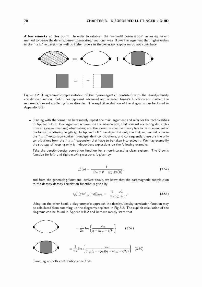
70 CHAPTER 3. DISORDERED LUTTINGER LIQUID
A few remarks at this point: In order to establish the “σ-model bosonization” as an equivalentmethod to derive the density/current generating functional we still owe the argument that higher ordersin the “ tr ln” expansion as well as higher orders in the generator expansion do not contribute.
= +
= +
Figure 3.2: Diagrammatic representation of the “paramagnetic” contribution to the density-densitycorrelation function. Solid lines represent advanced and retarded Green’s functions and dashed linerepresents forward scattering from disorder. The explicit evaluation of the diagrams can be found inAppendix B.2.
• Starting with the former we here merely repeat the main argument and refer for the technicalitiesto Appendix B.1. Our argument is based on the observation, that forward scattering decouplesfrom all (gauge invariant) observables, and therefore the effective theory has to be independent ofthe forward scattering length l0. In Appendix B.1 we show that only the first and second order inthe “ tr ln”-expansion contain l0-independent contributions, and consequently these are the onlycontributions from the “ tr ln ”-expansion that have to be taken into account. We may exemplifythe strategy of keeping only l0-independent expressions on the following example:
Take the density-density correlation function for a non-interacting clean system. The Green’sfunction for left- and right-moving electrons is given by
g±n (p) =1
−iǫn ± p− i2l0
sgn(n), (3.57)
and from the generating functional derived above, we know that the paramagnetic contributionto the density-density correlation function is given by
〈ρ+m(q)ρ+
−m(−q)〉para. = − 1
2π
ω2m
ω2m + q2
. (3.58)
Using, on the other hand, a diagrammatic approach the density/density correlation function maybe calculated from summing up the diagrams depicted in Fig.3.2. The explicit calculation of thediagrams can be found in Appendix B.2 and here we merely state that
=1
2πIm
ωm
q + iωm + i/l0
(3.59)
=1
2πIm
ωm
(ωml0 − iql0)(q + iωm + i/l0)
(3.60)
Summing up both contributions one finds

3.2. BOSONIZATION OF NON-INTERACTING ELECTRONS IN A CLEAN WIRE: THREEEQUIVALENT APPROACHES 71
Eq.(3.59) + Eq.(3.60) =1
2πIm
ωm
q + iωm
, (3.61)
i.e. Eq. (3.58). Instead of summing up both contributions, however, we may equally take a“short-cut” and set l0 to zero, which gives
Eq.(3.59) =−1
2πRe
ωml0
1 − iql0 + ωml0
= 0
Eq.(3.60) =1
2πIm
ωm
(ωm − iq)(ql0 + iωml0 + i)
=1
2πIm
ωm
iωm + q
,
i.e. the right result. We may thus take the short cut and set l0 = 0 right in the beginning; this issomewhat the strategy of keeping only l0-independent contributions from the “ tr ln ”-expansion.
• This leads us to the second remark concerning contributions from higher orders in the generators(“higher loop corrections” to the Gaussian propagator). In Appendix B.3 we argue that due tothe finite space-resolution set by the cut-off, Λ, used to regularize the momentum integrals, oneshould instead of using δ-distributed disorder better work with finite correlated Gaussian disorder,where the correlation length is given by Λ−1. Doing so one finds (see Appendix B.3) that theGaussian propagator is modified according to
〈Dffs,nn+m(x)Dff
s,n+mn(x′)〉S0
reg=
〈Dffs,nn+m(x)Dff
s,n+mn(x′)〉S0 , s(x− x′) > Λ−1
0, s(x− x′) < Λ−1.(3.62)
That is the propagator is unchanged on scales where the particle-hole excitation travels at leastthe distance Λ−1, but vanishes on smaller length scales. With this remark in mind we turn to thehigher loop corrections to the Gaussian propagator.
3.2.4 Higher loop corrections to the Gaussian propagator
We may now turn to the discussion of contributions from higher than second order in the generators.This point still needs further elaboration, and here I merely indicate a line of arguments which mightshow that all higher loop corrections to the Gaussian propagator vanish. Contributions from higherthan second order in the generators can be treated perturbatively with respect to the propagator fromthe Gaussian approximation, Eq.(3.62). These terms can be organized in a loop expansion where theloop order is given by the number of free momentum integrals. The lowest order corrections to theGaussian approximation result from terms which are fourth order in the generators, i.e. of the formS4[DD] = tr
ODDDD
, where O denotes the operator a, µ, ∂x, ∂τ , etc. For an operator which is
local in space, all fields D,D under a trace sit at the same space point and therefore no contractionscan be performed within one trace. Consider for example the contribution
〈trODDDD
trODDDD
〉S0
reg(3.63)
Performing Wick contraction on ends up with expressions
(
〈Dffs,nn+m(x)Dff
s,n+mn(x′)〉S0reg
)2
〈Dffs,nn+m(x′)Dff
s,n+mn(x)〉S0reg
(3.64)
which vanishes as it contains the product of propagators from x to x′ and from x′ to x. A systematicanalysis however still needs to be done in order to see if this argument generalizes to all contributionsfrom higher than second order in the generators. Especially a discussion of the lowest order corrections,〈trODD
trODDDD
〉S0
regand 〈tr
ODDDD
trODD
trODDDD
〉S0
regis still needed.

72 CHAPTER 3. DISORDERED LUTTINGER LIQUID
3.2.5 Summary of this section and outlook
In this section we showed that besides the well established standard and functional bosonization schemesone might apply a third method, the “σ-model bosonization”, in order to derive a generating functionalfor density/current correlation functions of the non-interacting, clean system. As already mentioned,the argument concerning the vanishing of higher loop corrections to the Gaussian propagators mayneed a critical revision. In the next section we show that even in the presence of e-e interactionsthe σ-model approach is equivalent to the former two approaches. The advantage of the “σ-modelbosonization” shows up when we introduce the stochastic backscattering disorder into the model. Thiswill be discussed in the subsequent sections. Before proceeding, however, we may summarize the threebosonization procedures discussed in this section in the following way:
1. The “standard bosonization approach” represents generating functional with help of a bosonicfield, i.e. ∫
d2xJ tΠJJ =
∫
d2xΘtΠ−1J Θ + J tΘ + ΘtJ,
2. the functional bosonization method uses the loop-cancellation in order to obtain from the “ tr ln”-expansion the generating functional
∫
d2xJ tΠJJ = tr ln
∂ + J
,
3. the “σ-model approach” uses the identity ΠJm(q) = 1 − ωm
q ΠJm(q) = 1 − iωmΠσ
m(q) in order toexpress the generating functional in terms of a matrix field, i.e.
∫
d2xJ tΠJJ =
∫
d2x trDqΠ−1
σ,m(q)D + J tD + DJ
+ J tJ.
Here J t =(µ+ ia, µ− ia
), ΠJ
m(q) = diag( qq+iωm
, qq−iωm
)and Πσ
m(q) = diag(
1|ωm|+iq ,
1|ωm|−iq
)
.
3.3 Interacting electrons in a clean wire: Equivalence of the
three approaches
Having exposed the σ-model bosonization for the clean non-interacting case we now want to show thatthe method also works for clean interacting systems. As our main focus, however, lies in disorderedsystems we merely give a brief sketch of the strategy followed in the case of clean interacting systemsand relegate more detailed calculations to Appendices B.4 and B.5. So let us start from the actiongiven in Eq.(3.8) and include Coulomb-interactions,
Sint.[χχ] =1
2
∫
d2x(ρ+ ρ−
)g
(ρ+
ρ−
)
. (3.65)
As discussed in section 1 we keep only the interaction between densities of opposite chirality and accountfor the interaction described by g4 by considering the renormalized Fermi-velocity, see Eq.(3.7). Theinteraction term is treated in the different bosonization schemes as follows:
3.3.1 Standard bosonization
In the standard bosonization scheme one employs that ρ± = 12π (∂xθ ∓ ∂xφ), in order to rewrite Sint.
in terms of the bosonic degrees of freedom,
Sint.[χχ] =g24π2
∫
d2x(∂xθ)
2 − (∂xφ)2. (3.66)
The bosonic action for the clean interacting system is therefore purely Gaussian in the bosonic fields,
3.3. INTERACTING ELECTRONS IN A CLEAN WIRE: EQUIVALENCE OF THE THREEAPPROACHES 73
S0[θ, φ] + Sint.[θ, φ] =1
2π
∑
km
(θmk φmk
)(
(1 + g22π )k2 iωmk
iωmk (1 − g22π )k2
)(θ−m,−kφ−m,−k
)
. (3.67)
Adding the source term, Ssou., given in Eq.(3.13) and integrating over the bosonic fields θ, φ one finds
S[a, µ] =1
2π
∑
m,q
vq2
v2q2 + ω2m
[gµmqµ−m,−q − g−1amqa−m,−q
]
+ωmq
v2q2 + ω2m
[µmqa−m,−q + amqµ−m,−q]
, (3.68)
where we introduced g =
√
1− g22π
1+g22π
and v =√
(1 + g22π )(1 − g2
2π ).
3.3.2 Functional bosonization
Working with the fermions, one decouples the interaction term with help of a Hubbard-Stratonovichtransformation. To this end one introduces the bosonic Hubbard-Stratonovich field ϕt =
(ϕ+ ϕ−),
with action
S[ϕ] =1
2
∫
d2xϕtg−1ϕ (3.69)
and shifts the field ϕ→ ϕ+ ig
(ρ+
ρ−
)
in order to obtain
S[ϕ] =1
2
∫
d2x
ϕtg−1ϕ−(ρ+ ρ−
)g
(ρ+
ρ−
)
− 2iχϕχ
,
where ϕ =
(ϕ−
ϕ+
)
. Combining the free and the interaction contributions one finds
S0[χχ] + Sint.[χχ] → S[ϕ] + S0[χχ, ϕ] =1
2
∫
d2x
ϕtg−1ϕ−∫
d2xχ [∂ + iϕ]χ
, (3.70)
which after integration over the fermionic fields leads to
S[ϕ] + Ssou.[µ, a] =1
2
∫
d2xϕtg−1ϕ+ tr ln ∂ + tr ln1 + G0 [µσ1 + aσ2 + iϕ]
. (3.71)
Expansion of the “ tr ln” (as in section 3) one simply has to shift the sources by the Hubbard-Stratonovich fields, i.e. J → J + ϕ, and finds
S[ϕ] + Ssou.[µ, a] =1
2
∫
d2xϕtg−1ϕ+ tr ln ∂ +1
2π
∫
d2x (J + ϕ)t Π(J + ϕ) , (3.72)
where we introduced the notation
J =
(µ+ iaµ− ia
)
and Πm(q) =
(Π+m(q)
Π−m(q)
)
with Π±m(q) =
q
q ± iωm. (3.73)
One can now show that Eq.(3.72) is equivalent to Eq.(3.68). This may be done by introduction of afurther bosonic field and, as it is rather technical, is postponed to Appendix B.4. At this point, however,

74 CHAPTER 3. DISORDERED LUTTINGER LIQUID
we want to mention that one can derive Eq.(3.72) also in a different manner: Instead of accounting forthe Hubbard-Stratonovich field in the “ tr ln ”-expansion one may also employ a gauge transformation,χs → χse
i(θ1+sθ2) and χs → e−i(θ1+sθ2)χs in order to remove the Hubbard-Stratonovich field fromthe action. Whereas the global (charge) U(1) gauge transformation (described by setting θ2 = 0)is unproblematic, the chiral U(1) gauge transformation (described by setting θ1 = 0) can only beimplemented by costs of an anomaly term (“chiral anomaly”, see e.g. [14]). This anomaly is exactlygiven by the polarization operator [14], Sanomaly = 1
2π
∫d2xϕtΠϕ.
3.3.3 σ-model bosonization
Proceeding as in the last subsection (i.e. decoupling the interaction by means of a Hubbard-Stratonovichtransformation) and following the same steps as in the clean case (we simply have to substitute J →J + ϕ in every step), one obtains after integration over the Diffusons
S[ϕ] + Ssou.[µ, a] =1
2
∫
d2xϕtg−1ϕ+ tr lnG−1
Λ
+
1
2π
∫
d2x (J + ϕ)tΠ(J + ϕ) . (3.74)
In order to show the equivalence to the functional bosonization method we therefore simply have toshow that tr ln
G−1
Λ
= tr ln ∂. Again, this rather technical step is postponed to the appendices
(see Appendix B.5).
3.3.4 Summary of this section
In this section we showed that interacting electrons in a clean 1d system can be described by the action
S = S[φ] + Sσ[T ] + Scoup[T, φ, J ] + Ssou[J ], (3.75)
where
S[φ] =1
2
∑
m,q
φtm(q)
(
g−1 − 1
2π
)
φ−m(−q) (3.76)
Sσ[T ] = −1
4
∑
nm,q
trΛnT
−1nn+m(q)Πσ
n+m(q)Tn+mn(−q)
(3.77)
Scoup[T, φ, J ] = −i(T
L
)1/2 ∑
nn′m
∑
q,k
tr
ΛnT−1nn′(q)
[
φm(k) + Jm(k)]
Tn′+mn(−q − k)
(3.78)
Ssou[J ] = − 1
4π
∑
m,q
J tm(q)J−m(−q). (3.79)
Notice that the “ tr” includes the trace over the ±-sector and we introduced the matrices T =(T+
T−
)
±and
Πσn+m(q) =
(ǫn+m + iq
ǫn+m − iq
)
±. The bosonic fields have the following structure in T⊗±-space
J(t) =
J+(t)J−(t)
J−(−t)J+(−t)
T⊗±
φ(t) =
φ+(t)φ−(t)
φ−(−t)φ+(−t)
T⊗±
,
(3.80)
where J± = µ± ia and correspondingly the vectors
J t(t) =(J+(t) J−(t) J−(−t) J+(−t)
)
T⊗± φt(t) =(φ+(t) φ−(t) φ−(−t) φ+(−t)
)
T⊗± .
(3.81)

3.4. INELASTIC SCATTERING RATE IN A CLEAN LUTTINGER LIQUID 75
3.4 Inelastic scattering rate in a clean Luttinger liquid
In a recent paper Gornyi et al. [5, 6] pointed out that, contrary to what one might expect due to thenon-Fermi liquid character of the Luttinger liquid, the notion of an inelastic scattering rate is finite andmeaningful even in the weakly interacting 1d system. The inelastic scattering rate is proportional to theimaginary part of the interaction induced self-energy, which is dominated by real inelastic processes, i.e.interaction processes involving real electron excitations, |ǫ| . T , and characteristic frequencies |ω| . T .To be precise, a second order (Golden Rule) calculation of the inelastic scattering-rate gives (see [5, 6]and below, Eq.(3.94))
1
τee=g22
4πT. (3.82)
Gornyi et al. compared the perturbative inelastic scattering rate, Eq.(3.82), to the damping of the exactsingle-particle Green’s function and found that the temporal decay for t → ∞ agrees with the GoldenRule expression [6]. That is, the temporal decay of the Green’s function is determined by the processesof inelastic scattering of right-movers on left-movers. Notice also that in the case of weak interactions(g2 ≪ 1) 1/τee is much smaller than temperature, i.e. Tτee ≫ 1. Gornyi et al. point out that thefact that the quasiparticle’s characteristic energy (|ǫ| . T ) is much larger than its lifetime, τee, is oneof the conditions for the existence of the Fermi-liquid state. “In this respect”, the authors conclude,“the weakly interacting Luttinger liquid, while being a canonical example of a non-Fermi liquid, revealsthe typical Fermi liquid property”[6]. The self-energy’s real part, on the other hand, is determined byhigh energy transfers |ω| & T , which is characteristic for elastic virtual processes. It is pointed out byGornyi et al. that it is specific to the 1d system that the real part of the self-energy is UV-divergent (itis logarithmically divergent in the ultraviolet and cut off by Λ) and the non-Fermi liquid physics of theLuttinger liquid is encoded in the singular real part of the (perturbative) self-energy.
In order to see how the σ-model for the clean interacting system works we briefly show how Eq.(3.82)can be obtained from Eq.(3.75). The Golden Rule calculation corresponds in the σ-model approach toan expansion to second order in generators. The second order expansion leads to the Diffuson action
Sσ[D] = − 1
2
∑
n,m
∑
q
tr
Dffnn+m(q)Πσ
|m|(q)Dffn+mn(−q)
θ(−n(n+m)) (3.83)
Scoup[D, φ] =iT 1/2∑
nm
∑
q
tr
ΛnDffnn+m(q)φf
−m(−q)
θ(−n(n+m))
+ 2i
(T
L
)1/2 ∑
mnn′
∑
pq
tr
ΛnDffnn′(p)Dff
n′n+m(−p− q)φfm(q)
θ(−nn′)θ(−n′(n+m)),
(3.84)
where Dff = diag(D+,ff, D-,ff
)
± and Πσ|m|(q) = diag
(|ωm| + iq sgn(m), |ωm| − iq sgn(m)
)
±. TheCooperon action, on the other hand, is given by
Sσ[C] = − 1
2
∑
mn
∑
q
tr
Cfbnn+m(q)Πσ
|m|(q)Cbfn+mn(−q)
θ(−n(n+m)) (3.85)
Scoup[C, φ] =2i
(T
L
)1/2 ∑
mnn′
∑
pq
tr
ΛnCfbnn′(p)Cbf
n′n+m(−p− q)φfm(q)
θ(−nn′)θ(−n′(n+m)).
(3.86)
Notice again, that since the Cooperon is off-diagonal in T-space, it does not couple linearly to theCoulomb-field, φ. Notice also that in Eq. (3.83) - Eq. (3.85), the bosonic fields are those on theforward time-branch (the first component in T-space). In the following we will suppress the T-spaceindex, i.e. φ = φf.

76 CHAPTER 3. DISORDERED LUTTINGER LIQUID
3.4.1 Screening the Coulomb-interactions
The peculiarity of a clean Luttinger liquid is that the RPA approximation for the dynamically screenedinteraction is exact (we already mentioned the cancelation of higher loop contributions in the “tr ln”expansion in section 3.2.2). We briefly show how the RPA screening is obtained from Eq.(3.84). Withthe RPA screened Coulomb propagator we then derive Eq.(3.82).
The Coulomb interactions are screened by virtual particle-hole excitations. This effect is containedin the coupling of the photon-field, φ, to the “linear” particle-hole excitation, i.e. the “linear” Diffuson,D (first line in Eq.(3.84)). Performing the integral over the linear D with respect to the Gaussian actionwe obtain
〈Scoup[D, φ]Scoup[D, φ]〉= −T
∑
nmn′m′
∑
qq′
〈tr
ΛnDffnn+m(q)φ−m(−q)
tr
Λn′Dffn′n′+m′(q′)φ−m′(−q′)
〉
θ(−n(n+m))θ(−n′(n′ +m′))
=1
2π
∑
s=±
∑
m
∑
q
|ωm||ωm| + isq sgn(m)
φsm(q)φs−m(−q)
=1
2π
∑
s=±
∑
m
∑
q
φtm(q)
( |ωm||ωm|+iq sgn(m)
|ωm||ωm|−iq sgn(m)
)
φ−m(−q).
Adding 12 〈ScoupScoup〉 to the photon action, S[φ], one finds the screened photon propagator,
S[φ] =1
2
∑
m,q
φtm(q)
(
g−1 − 1
2πΠφm(q)
)
φ−m(−q), (3.87)
with the polarization matrix
Πφm(q) =
(iq sgn(m)
|ωm|+iq sgn(m)−iq sgn(m)
|ωm|−iq sgn(m)
)
=
( qq−iωm
qq+iωm
)
. (3.88)
As we restrict our analysis to weak interactions we may perform an expansion in g2 ≪ 1 to find thephoton propagators (again φ = φf)
〈φ+m(q)φ+
−m(−q)〉 =g22
2π
q
q + iωm
1 +g22
4π2
q2
q2 + ω2m
+ ...
(3.89)
〈φ−m(q)φ−−m(−q)〉 =g22
2π
q
q − iωm
1 +g22
4π2
q2
q2 + ω2m
+ ...
(3.90)
〈φ+m(q)φ−−m(−q)〉 = g2
1 +g22
2π
q2
q2 + ω2m
+ ...
. (3.91)
3.4.2 The inelastic scattering rate
The Coulomb interaction causes inelastic scattering between electrons, and leads to a finite life-time ofthe quasi-particles. As mentioned in the introduction the concept of a quasi-particle life time makes alsosense for the Luttinger liquid and, for the weakly interacting case, may be obtained from a perturbativecalculation of the self-energy. In the σ-model approach the lowest order contribution to the self-energy isobtained from an expansion of the quadratic (in D, C respectively) coupling term (first line in Eq.(3.84)

3.4. INELASTIC SCATTERING RATE IN A CLEAN LUTTINGER LIQUID 77
and Eq.(3.86)) to second order followed by a contraction in D, C respectively; i.e.
1
2〈Scoup[D, φ]Scoup[D, φ]〉
=2T
L
∑
mm′n1,...,n4
∑
pp′qq′
〈tr
Λn1Dffn1n2
(p)Dffn2n1+m(−p− q)φm(q)
tr
Λn3Dffn3n4
(p′)Dffn4n3+m′(−p′ − q′)φm′ (q′)
〉Sσ
=4T
L
∑
s=±
∑
mn1n2
∑
qp
φsm(p)φs−m(−p)|ωm| + sip sgn(m)
[θ(n1(n1 +m)) + θ(n1(n1 −m)) + 2δm,0] trDs,ffn1n2
(q)Ds,ffn2n1
(−q)
− φsm(p)φs−m(−p)|ωm| + sip sgn(m)
[
θ(n1(n1 +m))θ(n2(n2 +m)) trDs,ffn1n2
(q)Ds,ffn2+mn1+m(−q)
+ 2δm,0 trDs,ffn1n2
(q)Ds,ffn2n1
(−q)]
.
Here we set the Diffuson frequency (ωm = ǫn1−n2) and momentum (q = p − p′) to zero since theinelastic scattering rate is, by definition, the mass term, i.e. the self-energy at zero momentum andfrequency. Expansion of the self-energy in powers of ωm and q, one finds quantum corrections to thediffusion constant, the density of states, and the frequency [15, 16]. The bosonic frequency summation,m, is restricted to values such that the interaction process only involves electron-hole pairs. The firstline contains the “pure” self-energy contribution and the second line contains the vertex contributions(see also Chapter 2 “Dephasing due to magnetic impurities”).
For the Cooperon, one obtains similarly
1
2〈Scoup[C, φ]Scoup[C, φ]〉
=2T
L
∑
mm′n1,...,n4
∑
pp′qq′
〈tr
Λn1Cfbn1n2
(p)Cbfn2n1+m(−p− q)φm(q)
tr
Λn3Cfbn3n4
(p′)Cbfn4n3+m′(−p′ − q′)φm′ (q′)
〉Sσ
=4T
L
∑
s=±
∑
mn1n2
∑
qp
φsm(p)φs−m(−p)|ωm| + sip sgn(m)
[θ(n1(n1 +m)) + θ(n1(n1 −m)) + 2δm,0] trCs,fbn1n2
(q)Cs,bfn2n1
(−q)
− φsm(p)φ−s−m(−p)|ωm| + sip sgn(m)
[
θ(n1(n1 +m))θ(n2(n2 +m)) trCs,fbn1n2+m(q)Cs,bf
n2n1+m(−q)
+ 2δm,0 trCs,fbn1n2
(q)Cs,bfn2n1
(−q)]
.
Again, the first line gives the “pure” self-energy and the second line the vertex contributions. Noticethat the energy-structure of the vertex-contribution is different for the Diffuson and Cooperon. Indeed,the energy structure for the Diffuson is such, that self-energy and vertex contributions exactly cancel (nodephasing in one loop), whereas for the Cooperon vertex contributions cancel only interaction processesfrom the self-energy involving small energies, ω . 1/τϕ, see Appendix B.6 and Chapter 2 (“Dephasingdue to magnetic impurities”.)
As already mentioned, the inelastic scattering rate is obtained from the self-energy contribution only.It is (for Diffuson and Cooperon) given by
1
τsinel.(ǫn)=
4T
L
∑
m
∑
q
Πsm(q)V s
m(q) [θ(n(n+m)) + θ(n(n−m))] ,

78 CHAPTER 3. DISORDERED LUTTINGER LIQUID
where Πsm(q) = 1
|ωm|+sip sgn(m) and we introduced V sm(q) = 〈φsm(p)φs−m(−p)〉. The analytical con-
tinuation gives
∑
m
Πsm(q)V s
m(q) [θ(n(n+m)) + θ(n(n−m))]
= − 2
πT
∫
dΩ
(
coth[ Ω
2T
]ImV R,s
Ω (q) +1
2itanh
[ǫ− Ω
2T
]V R,s
Ω (q) +1
2itanh
[ǫ+ Ω
2T
]V A,s
Ω (q)
)
ΠR,sΩ (q)
+1
πT
∫
dΩ
(1
2itanh
[ǫ− Ω
2T
]V R,s
Ω (q) +1
2itanh
[ǫ+ Ω
2T
]V A,s
Ω (q)
)
ΠR,sΩ (q), (3.92)
where we also analytically continued iǫn → ǫ. The contribution in the second line describes high-energyǫ,Ω & T processes with virtual electrons involved (see discussion of the beginning of this section).These combine with diagrams where the analytical structure of a single particle line is changed duethe interaction process (i.e. with diagrams not considered here) to describe corrections to the diffusionconstant, see e.g. [17]. That is, they are not relevant for inelastic scattering processes which only includereal electrons (i.e. electrons with energy ǫ . T ) and will be dropped out in the following. The remainingterm involves only processes with energy transfer Ω . T (i.e. real inelastic processes). This is guaranteedby the combination of thermal functions. Notice also, that, since only the imaginary part of the screenedCoulomb interaction, ImV , enters the inelastic scattering rate, the diamagnetic contribution from thepolarization operator vanishes and only its paramagnetic part contributes. Taking into account onlyelectrons at the Fermi energy (ǫ = 0) and using that coth
[Ω2T
]− tanh
[Ω2T
]= 2 sinh−1
[ΩT
]and
ΠR,s−Ω(−q) = ΠA,s
Ω (q) and V R,s−Ω(−q) = V A,s
Ω (q) one finds
1
τinel.(ǫ = 0)= − 2
Lπ
∑
q
∫
dΩ1
sinh[
ΩT
] ImV R,sΩ (q)Re ΠR,s
Ω (q). (3.93)
With the RPA screened propagator, Eq.(3.89) - Eq.(3.91), analytically continued to real frequencies,
V R,sΩ (q) =
g222π
qq+sΩ+si0 and ΠR,s
Ω (q) = −isq−Ω−i0 one finds the inelastic scattering rate
1
τsinel.(ǫ = 0)=g22
π2
∫dq
2π
∫
dΩ1
sinh[
ΩT
] Imq
q + sΩ + si0Im
1
sq − Ω − i0
= − sg22
2π
∫
dq
∫
dΩq
sinh[
ΩT
]δ(q + sΩ)δ(sq − Ω)
=g22T
2π
∫
dq
∫
dΩδ(q + sΩ)δ(q − sΩ)
=g22
4πT. (3.94)
3.4.3 Summary of this section
In this section we showed how the σ-model works at the example of the inelastic dephasing rate ina clean Luttinger liquid. More important, we repeated the observations of Gornyi et al. [5, 6] thatit is the elastic virtual processes, which are determined by interaction processes with high energiesΩ & T , which lead to the non-Fermi liquid singularities typical for the Luttinger liquid. The inelastic
real processes, on the other hand, (involving interaction processes with energy transfer Ω . T ) lead tofinite and meaningful results, as e.g. for the quasi-particle life-time. We will come back to the GoldenRule calculation of the inelastic scattering rate when we interpret the dephasing rate which governs thedecay of the persistent current in a disordered Luttinger liquid, see section 3.7.2.
3.5 Electrons in a disordered one-dimensional system
As stated in the introduction, our main focus lies on disordered one-dimensional systems. We alreadymentioned that including arbitrary weak (stochastic) disorder in the “standard” or the “functional”bosonization schemes leads to theories disparate more complicated. In this section we want to show

3.5. ELECTRONS IN A DISORDERED ONE-DIMENSIONAL SYSTEM 79
how stochastic disorder can be treated within the σ-model bosonization. To this end we restrict ourselvesin this section to the non-interacting case. That is we start out from the action Eq.(3.8) and includeback-scattering disorder described by
Sv[χχ] = −∫
d2xχvσ1χ, 〈v(x)v(x′)〉 = l−11 . (3.95)
Notice that compared to Eq. (3.6) we work in the rotated basis, as introduced in section 3. Goingthrough the steps of section 3. integrating out the electrons leads to (compare with Eq.(3.32))
S[T ] = −1
2tr ln 1 + GΛ[X1 +X2 +X3] , (3.96)
where X3nn′(x) = [T−1vσ1T ]nn′(x). In Appendix B.7 we show that expansion of the “ tr ln” gives only
one contribution involving X3, which comes from the second order “ tr ln ”-expansion, i.e. S(2)[T ] =Sbs[T ], where
Sbs[T ] = − 1
16l1
∑
nn
tr[TΛT−1]nn′(q)σ1[TΛT−1]n′n(−q)σ1
. (3.97)
Therefore, non-interacting electrons in a disordered wire are described by the action
S = Sσ[T ] + Sbs[T ] + Scoup[T, J ] + Ssou[J ], (3.98)
where
Sσ[T ] = −1
4
∑
nm,q
trΛnT
−1nn+m(q)Πσ
m(q)Tn+mn(−q)
(3.99)
Sbs[T ] = − 1
16l1
∑
nn′
trσ1[TΛnT
−1]nn′(q)σ1[TΛT−1]n′n(−q)
(3.100)
Scoup[T, J ] = −i(T
L
)1/2 ∑
nn′m
∑
q,k
tr
ΛnT−1nn′(q)Jm(k)Tn′+mn(−q − k)
(3.101)
Ssou[J ] = − 1
4π
∑
m,q
J tm(q)J−m(−q), (3.102)
with T , Πσm(q), J and J as in the last section. That is, the inclusion of backscattering disorder leads to
a coupling of the ballistic σ-model actions for the left- and right -moving particle-hole excitations (i.e.for the +- and −-branches). As we will see below this innocent looking coupling renders the modelmuch more complicated, since e.g. in a perturbative evaluation one has to account for contributionsfrom higher than second order.
3.5.1 Localization in a disordered 1d system
The model Eq.(3.97) shows nicely that in a non-interacting system (i.e. where phase coherence is notdestroyed by inelastic scattering processes) the ballistic motion on short scales crosses over directly intothe localization regime, with no diffusive dynamics on intermediate length scale. This may be seen asfollows: We parametrize rotations by a massless “center-of-mass”- and a massive “relative”-coordinate,T± = e±KT0, and perform an expansion to second order in the “relative”-coordinate, K,
S = Sσ[K,T0] + Sbs[K] + Scoup[K,T0, a, µ] + Ssou[J ], (3.103)

80 CHAPTER 3. DISORDERED LUTTINGER LIQUID
where
Sσ[K,T0] =1
2
∫
dτdτ ′dx tr(
1 − 2K2)ΛT−1
0 i∂τT0 −KΛT−10 ∂xT0
(3.104)
Sbs[K] = −l−11
∫
dτdτ ′dx trK2
(3.105)
Scoup[K,T0, µ, a] = −2i
∫
dτdτ ′dx tr(
1 − 2K2)ΛT−1
0 µT0 − 2iKΛT−10 aσT
3 T0
(3.106)
Ssou[J ] = − 1
4π
∫
d2xJ tJ. (3.107)
Integration over the massive quadraticK fluctuations one finds (For strong disorder l1 → 0 theK-actionis governed by its saddle-point K = 0 and small fluctuations around it)
Sbs[K] + Sσ[K,T0] + Scoup[K,T0, µ, a]
≈ −l−11
∫
dτdτ ′dx trK2− 1
2
∫
dτdτ ′dx trKΛT−1
0
[∂x + 8aσT
3
]T0
→ l12
∫
dτdτ ′dx tr(
ΛT−10
[∂x − 8aσT
3
]T0
)2
.
Adding the K-independent terms we end up with the diffusive σ-model in the “center-of-mass” co-ordinate T0,
Sσ[Q, a, µ] =1
2
∫
dτdτ ′dx tr
(i∂τ + µ)Q− l1(∂x + i[aσT
3 , .]Q)2
, (3.108)
where Q = T−10 ΛT0. Notice that while in higher dimension the derivation of the diffusive σ-model
relies on a gradient expansion, which makes use of the small parameters ωmτ,Dq2τ ≪ 1 (see Chapters1 and 2), the above derivation does not make any use of this presumption.
Even more important, the higher dimensional σ-model has a regime of “weak disorder” in which thelargeness of the parameter ǫFτ ≫ 1 (weak disorder) allows for a perturbative expansion in generators.This allows for a systematic organization of quantum corrections to e.g. the classical Drude conductivity(to be more precise, in 2d and quasi 1d systems one also has to assume that quantum corrections arecut-off by some dephasing mechanism, see Chapters 1 and 2). In contrast to this, Eq.(3.108) lacksof a global large parameter allowing for a perturbative expansion in the generators. Therefore, largefluctuations of the Q-field (describing the proliferation of particle-hole excitations) are not suppressedand cause Anderson localization [1]. The ballistic motion on short length scales crosses over into thelocalized regime, without diffusive intermediate regime.
3.5.2 Drude conductivity and weak localization in a disordered 1d system
In their recent work Gornyi et al. [5, 6] showed that key notions of mesoscopic physics, such as weaklocalization and dephasing are also applicable to disordered (interacting) one-dimensional systems. Tobe precise, the authors showed that in the regime of relatively high temperatures, where the dephasing-time, τϕ, due to e-e interactions is much smaller than the mean free path, l1, of the forward scatteringdisorder interference corrections to the Drude conductivity (signaling the onset of Anderson localization)can be organized in a perturbative expansion with expansion parameter τϕ/l1. In this subsection webriefly indicate how this may be seen within the σ-model without presenting a more careful analysis.
Drude conductivity: The Drude conductivity, σD = l1π , is obtained from Eq.(3.108) by insertion
of the saddle point value Q = Λ (see Chapters 1 and 2). In section 3.6.2 we show that virtual
elastic e-e interaction processes renormalize the backscattering length, l1, leading to a temperaturedependent Drude conductivity (see Eq.(3.144)). At moderately high temperatures it is however theweak localization corrections to the Drude conductivity that govern the temperature dependence ofthe conductivity for the case of weak e-e interactions (compare Eq.(3.112) and Eq.(3.143)) and, withlowering the temperature, eventually drive the system into the strong localization regime. So let usbriefly discuss the interference corrections to the Drude conductivity.

3.5. ELECTRONS IN A DISORDERED ONE-DIMENSIONAL SYSTEM 81
Interference corrections to the Drude conductivity: arise due to coherent backscattering processesand in the higher dimensional systems can be obtained from Eq.(3.108) by a systematic expansion ingenerators, Q = Λ (1 +W + ...) (as discussed in Chapters 1 and 2) We already mentioned that, incontrast to its higher dimensional relatives, such a perturbative expansion in generators is not justifiedin the noninteracting one-dimensional system. Assuming however strong dephasing, such that τϕ ≪ l1,quantum corrections to the Drude conductivity are strongly suppressed. Weak localization correctionsare then given by a minimal loop consisting of three scattering events [5, 6].
Technically, one may introduce a dephasing rate 1/τϕ ≫ 1/l1, and expand action Eq.(3.98) tosecond order in the generators. This leads to the ballistic ±-Cooperon propagator
Πσ,l1|m| (q) =
(|ωm| + iq sgn(m) + l−11 + τ−1
ϕ 1/l11/l1 |ωm| + iq sgn(m) + l−1
1 + τ−1ϕ
)
. (3.109)
A systematic expansion in the off-diagonal coupling term amounts to an expansion in the parameterτϕ/l1. In the limit of strong dephasing, τϕ ≪ l1 the weak localization corrections to the Drudeconductivity are dominated by a loop consisting of three scattering events, which is the minimal numberto from a loop [5, 6], i.e.
∆σ3WL ∝σDl−2
1
∑
−m<n<0
∫
dq1
q + i/τϕ
1
q − i/τϕ
1
q + i/τϕ, (3.110)
and leads to
∆σ3WL ∝ σD
(τϕl1
)2
. (3.111)
Accordingly, a kth-order scattering processes (the “k-Cooperon”) gives interference corrections to the
Drude conductivity of the order ∆σkWL ∝ σD(τϕ
l1
)k
. Notice however, that in the case where dephasing is
due to electron-electron interactions, a more careful analysis, reveals that WL corrections are dominatedby contributions of rare configurations in which two of the three impurities are anomalously close toeach other [5, 6]. In these configurations the dephasing is strongly suppressed (since the impurities
are close to each other) and [5, 6] ∆σWL ∝(τϕ
l1
)2
ln l1τϕ
. In any case, lowering the temperature
decreases the dephasing rate (for e-e interactions this happens more rapidly than the renormalizationof the backscattering length), such that finally τϕ ∼ l1 marks the cross over temperature where stronglocalization sets in. Let us briefly mention that for weak electron-electron interactions the dephasingrate measured in the weak localization experiment is given by [5, 6]
1
τϕ=g22
√T
πl1. (3.112)
3.5.3 Summary of this section
In this section we derived an effective field theory for the non-interacting disordered 1d system. Weshowed how in the absence of any interactions (leading to dephasing due to inelastic processes), theballistic propagation of electron-hole pairs on short scales crosses over directly into the localizationregime, with no diffusive dynamics on intermediate length scales. Technically, considering length scalesgreater than l1 scattering between the ±-branches becomes effectual and the field theory for the twoindependent branches gets locked into a single copy. We repeated recent arguments by Gornyi thatfor interacting systems there exists a regime (of moderate high temperatures) where the conductiv-ity is dominated by the Drude conductivity (with temperature-dependent renormalized backscatteringlength) and interference corrections, which can be organized in an perturbative expansion. Introducingphenomenologically a dephasing rate we indicated how these results can be obtained within the σ-model.
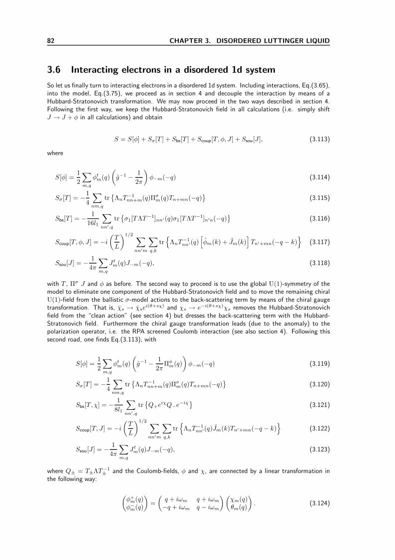
82 CHAPTER 3. DISORDERED LUTTINGER LIQUID
3.6 Interacting electrons in a disordered 1d system
So let us finally turn to interacting electrons in a disordered 1d system. Including interactions, Eq.(3.65),into the model, Eq.(3.75), we proceed as in section 4 and decouple the interaction by means of aHubbard-Stratonovich transformation. We may now proceed in the two ways described in section 4.Following the first way, we keep the Hubbard-Stratonovich field in all calculations (i.e. simply shiftJ → J + φ in all calculations) and obtain
S = S[φ] + Sσ[T ] + Sbs[T ] + Scoup[T, φ, J ] + Ssou[J ], (3.113)
where
S[φ] =1
2
∑
m,q
φtm(q)
(
g−1 − 1
2π
)
φ−m(−q) (3.114)
Sσ[T ] = −1
4
∑
nm,q
trΛnT
−1nn+m(q)Πσ
m(q)Tn+mn(−q)
(3.115)
Sbs[T ] = − 1
16l1
∑
nn′,q
trσ1[TΛT−1]nn′(q)σ1[TΛT−1]n′n(−q)
(3.116)
Scoup[T, φ, J ] = −i(T
L
)1/2 ∑
nn′m
∑
q,k
tr
ΛnT−1nn′(q)
[
φm(k) + Jm(k)]
Tn′+mn(−q − k)
(3.117)
Ssou[J ] = − 1
4π
∑
m,q
J tm(q)J−m(−q), (3.118)
with T , Πσ J and φ as before. The second way to proceed is to use the global U(1)-symmetry of themodel to eliminate one component of the Hubbard-Stratonovich field and to move the remaining chiralU(1)-field from the ballistic σ-model actions to the back-scattering term by means of the chiral gaugetransformation. That is, χs → χse
i(θ+sχ) and χs → e−i(θ+sχ)χs removes the Hubbard-Stratonovichfield from the “clean action” (see section 4) but dresses the back-scattering term with the Hubbard-Stratonovich field. Furthermore the chiral gauge transformation leads (due to the anomaly) to thepolarization operator, i.e. the RPA screened Coulomb interaction (see also section 4). Following thissecond road, one finds Eq.(3.113), with
S[φ] =1
2
∑
m,q
φtm(q)
(
g−1 − 1
2πΠφm(q)
)
φ−m(−q) (3.119)
Sσ[T ] = −1
4
∑
nm,q
trΛnT
−1nn+m(q)Πσ
m(q)Tn+mn(−q)
(3.120)
Sbs[T, χ] = − 1
8l1
∑
nn′,q
trQ+e
iχQ−e−iχ (3.121)
Scoup[T, J ] = −i(T
L
)1/2 ∑
nn′m
∑
q,k
tr
ΛnT−1nn′(q)Jm(k)Tn′+mn(−q − k)
(3.122)
Ssou[J ] = − 1
4π
∑
m,q
J tm(q)J−m(−q), (3.123)
where Q± = T±ΛT−1± and the Coulomb-fields, φ and χ, are connected by a linear transformation in
the following way:
(φ+m(q)φ−m(q)
)
=
(q + iωm q + iωm−q + iωm q − iωm
)(χm(q)θm(q)
)
. (3.124)

3.6. INTERACTING ELECTRONS IN A DISORDERED 1D SYSTEM 83
Depending on the situation it is more comfortable to work with either action. The above model is thesingle channel limit of a recently developed low-energy field theory of weakly disordered multi-channelconductors [7], which in the limit of small energies ǫ < τ−1
0 (τ−10 being the bare elastic scattering rate)
and a large number of transport channels recovers Finkel’stein’s diffusive interacting σ-model [2] withall known consequences.
3.6.1 RPA screening in a disordered system
As a first application of Eq.(3.113) let us see how the RPA screening is changed due to disorder. Thesecalculations show that the life-time of the particle-hole excitations responsible for the RPA screening ofthe Coulomb interactions becomes finite. This leads to non-vanishing dephasing rates determining themagnitude of the WL (see [5, 6]) and the amplitude of the persistent current (see end of section 3.7.2)in a disordered Luttinger liquid.
This is most conveniently done in the representation Eq.(3.114) - Eq.(3.118). We already saw (insection 4) that the RPA-screening is obtained from integrating over the expression in the action, wherethe “linear” Diffuson couples to the Coulomb field. Expansion of Eq.(3.114) - Eq.(3.118) to secondorder in the Diffusons we obtain
S[D] = Sσ[D] + Sbs[D] + Scoup[D, φ], (3.125)
where
Sσ[D] + Sbs[D] = − 1
2
∑
n,m
∑
q
tr
[Dff]tnn+m(q)Πσ,l1|m| (q)Dff
n+mn(−q)
θ(−n(n+m)) (3.126)
Scoup[D, φ] =iT 1/2∑
nm
∑
q
tr
ΛnDffnn+m(q)φ−m(−q)
θ(−n(n+m))
+ 2i
(T
L
)1/2 ∑
mnn′
∑
pq
tr
ΛnDffnn′(p)Dff
n′n+m(−p− q)φm(q)
θ(−nn′)θ(−n′(n+m)),
(3.127)
with
Πσ,l1|m| (q) =
(|ωm| + iq sgn(m) + l−1
1 −l−11
−l−11 |ωm| − iq sgn(m) + l−1
1
)
±and Dt =
(D+ D−)
± .
Proceeding as in section 4, the polarization operator, providing the RPA screening, is obtained in thefollowing way:
〈Scoup[D, φ]Scoup[D, φ]〉
=1
2π
∑
s,s′=±
∑
nm
∑
q
[Πσ,l1
]−1
ss′,m(q)φsm(q)φs
′
−m(−q)θ(−n(n+m))
=1
2π
∑
s=±
∑
m
∑
q
φtm(q)|ωm|
(|ωm| + l−11 )2 + q2 − l−2
1
(|ωm| − iq sgn(m) + l−1
1 l−11
l−11 |ωm| + iq sgn(m) + l−1
1
)
φ−m(−q)
=1
2π
∑
s=±
∑
m
∑
q
φtm(q)|ωm|
|ωm|2 + q2 + 2|ωm|l−11
(|ωm| − iq sgn(m) + l−1
1 l−11
l−11 |ωm| + iq sgn(m) + l−1
1
)
φ−m(−q).
Adding 12 〈ScoupScoup〉 to the photon action S[φ] therefore gives
S[φ] =1
2
∑
m,q
φtm(q)
(
g−1 +1
2π− 1
2πΠφm(q)
)
φ−m(−q), (3.128)

84 CHAPTER 3. DISORDERED LUTTINGER LIQUID
with the polarization
Πφm(q) =
|ωm||ωm|2 + q2 + 2|ωm|l−1
1
(|ωm| − iq sgn(m) + l−1
1 l−11
l−11 |ωm| + iq sgn(m) + l−1
1
)
, (3.129)
and
1 − Πφm(q) =
1
q2 + |ωm|2 + 2|ωm|l−11
(q2 + |ωm|l−1
1 + iωmq |ωm|l−11
|ωm|l−11 q2 + |ωm|l−1
1 + iωmq
)
. (3.130)
Notice that the polarization operator, Eq.(3.129), aquires Eq.(3.88) in the clean limit l−11 → 0 and the
conventional diffusion pole 1/(Dq2 + |ωm|) in the limit |ωm| ≪ l−11 , q, where the 1d diffusion constant
D = l1/2 (we use vF = 1).For weak interactions g2 ≪ 1 and we may expand,
〈φsφs′〉 = gss′ −[g(1 − Πφ
)g]
ss′+O(g3
2) (3.131)
leading to the photon propagators
〈φ+m(q)φ+
−m(−q)〉 =g22
2π
(
1 − iωm
q + iωm + il−11 sgn(m)
)
+O(g42) (3.132)
〈φ−m(q)φ−−m(−q)〉 =g22
2π
(
1 − −iωmq − iωm − il−1
1 sgn(m)
)
+O(g42) (3.133)
〈φ+m(q)φ−−m(−q)〉 = g2 +
g22
2π
l−11 |ωm|
q2 + (|ωm| + l−11 )2
+O(g32). (3.134)
3.6.2 “Renormalization” of disorder by electron-electron interactions
Let us now turn to the renormalization of the static disorder scattering length due to electron-electroninteractions. The only peculiarity of the Luttinger liquid as compared to higher dimensions is that therenormalization of the (back-) scattering length is more singular and necessitates going beyond theHartree-Fock approximation even in the case of weak interactions [5, 6]. The renormalization occursdue to elastic virtual electron-hole excitations involving virtual electron states with energies |ǫ| & T andtypical energy transfers |ω| & T . The underlying physics of the elastic renormalization of disorder canbe described in terms of the T -dependent screening of individual impurities and scattering by slowlydecaying in real space Friedel oscillations [18]. I want to point out, however, that a complete under-standing of the renormalization of the backscattering length still requires an investigation of the roleplayed by particle-hole fluctuations (Notice that in the standard bosonization scheme, also (bosonized)electrons renormalize the backscattering length. In the present approach a similar contribution mayresult from “high-energy” contributions of the Q-fields).
The renormalization of disorder is most conveniently treated within the representation Eq.(3.119) -Eq.(3.123). In a first step we represent the Coulomb-action, Eq.(3.119), in terms of the gauge fields θand χ. Using Eq.(3.124) we find that
S[θ, χ] =1
2
∑
m,q
(θm(q) χm(q)
)( 1g2
(q2 + ω2m) − 1
2π q2 − 1
2π iωmq
− 12π iωmq
−1g2
(q2 + ω2m) − 1
2π q2
)(θ−m(−q)χ−m(−q)
)
.
(3.135)
Introducing vJ = 1 − g22π and vN = 1 + g2
2π and integrating over θ gives
S[χ] =1
2g2
∑
m,q
χm(q)
[(q2 + ω2
m)(vJvNq2 + ω2
m)
vJq2 + ω2m
]
χ−m(−q). (3.136)

3.6. INTERACTING ELECTRONS IN A DISORDERED 1D SYSTEM 85
Motivated by the observation that the renormalization of the static disorder occurs due to virtualelectron-hole excitations we proceed by decomposing the Coulomb-field into its slow and fast fluctuatingcontributions, χτ (q) = χs
τ (q) + χfτ (q), where
χsτ (q) =
1
2πT 1/2
∫
|ω|<Tdωeiωτχω(q), (3.137)
χfτ (q) =
1
2πT 1/2
∫
T<|ω|<Λ
dωeiωτχω(q). (3.138)
Here we used the continuum approximation for frequencies (we want to study high energies ω & T ), andsubstituted the discrete sums by integrals. In order to integrate out the fast fields we use a perturbativeapproach and approximate
e−Seffbs [T,χs] ≈ e−Sbs[T,χs]e−〈Sbs[T,χs,χf]〉f ,
with the average 〈...〉f taken with respect to fast Coulomb-field action,
S[χf] =1
2g2
∑
m,q
χm(q)
[(q2 + ω2
m)(vJvNq2 + ω2
m)
vJq2 + ω2m
]
χ−m(−q) (3.139)
=L
8π2Tg2
∫
dq
∫
T<|ω|<Λ
χfω(q)
[(q2 + ω2)(vJvNq
2 + ω2)
vJq2 + ω2
]
χf−ω(−q) (3.140)
≡ 1
2
∫
dq
∫
T<|ω|<Λ
χfω(q) [Πχ]
−1ω (q)χf
−ω(−q). (3.141)
For high energies ǫn, ǫn′ & T slow and fast fields do not couple, i.e.
Sbs[T, χ] = − 1
8l1
∫
dτdτ ′dx trQ+e
iχQ−e−iχ
= − 1
8l1
∫
dτdτ ′dx tr
Q+ττ ′(x)e
iχsτ (x)Q−
τ ′τ (x)e−iχs(x)τ′
eiχfτ (x)−iχf
τ′ (x),
and therefore 〈Sbs[T, χs, χf]〉f = 〈eiχfτ (x)−iχf
τ′ (x)〉f. Using that
ln[
〈eiχfτ (x)−iχf
τ′ (x)〉f]
=L
16π4T
∫
dq
∫
T<|ω|<Λ
dωΠχω(q) [1 − cos[ω(τ − τ ′)]]
=g24π2
∫
dq
∫
T<|ω|<Λ
dωvJq
2 + ω2
(q2 + ω2)(vJvNq2 + ω2)
=g24π
∫
T<|ω|<Λ
dω1
|ω|
[1 − vJ
1 − vJvN+
√vJ
vN
1 − vN
1 − vJvN
]
=1
2
∫
T<|ω|<Λ
dω1
|ω|
[
1 −√
1 − g22π
1 + g22π
]
= α ln
[Λ
T
]
,
where α = 1 −√
1− g22π
1+g22π
and reexponating one finally finds 〈Sbs[T, χs, χf]〉f =(
ΛT
)α, i.e. the former
back-scattering term,
Seffbs [T, χs] = Sbs[T, χs]〈Sbs[T, χf]〉f = − 1
8leff1
∫
dτdτ ′dx trQ+e
iχQ−e−iχ , (3.142)

86 CHAPTER 3. DISORDERED LUTTINGER LIQUID
with the renormalized scattering length
1
leff1=
1
l1
(Λ
T
)α
, α = 1 −√
1 − g22π
1 + g22π
. (3.143)
Taking into account the renormalization of disorder by virtual electron-hole pairs, the Drude conductivity,mentioned in section 3.5.2, shows the following temperature dependence,
σD ∝(
Λ
T
)α
. (3.144)
3.6.3 Summary of this section and outlook
In this section we introduced the σ-model for the interacting disordered 1d system. We showed, onthe one hand, how the RPA screening is changed due to disorder and, on the other hand, how theback-scattering length is renormalized by interactions. The latter leads to a T -dependence of the Drudeconductivity. We emphasized that the derived σ-model represents the single-channel version of a multi-channel model, recently given by Mora et al. [7], which describes the physics of quasi-1d and higherdimensional systems. Therefore, the coupled ballistic σ-model can be viewed as an “universal” modelfor interacting disordered systems. As already pointed out, the role of “high energy” fluctuations of theQ-matrices in the renormalization of the backscattering length still needs to be discussed.
3.7 An Application: Persistent current in a Luttinger liquid
We already mentioned at different points the work of Gornyi et al. [5, 6], showing that conceptsfrom multi-channel disordered mesoscopic systems, also apply to the disordered Luttinger liquid. To beprecise, the work of Gornyi et al. concentrates on the WL corrections to the Drude conductivity. In thissection we want to discuss a further prominent example of an interference phenomenon, well known fordisordered mesoscopic systems and, up to now, not analyzed in single channel disordered rings. This isthe persistent equilibrium current produced by a Aharonov-Bohm (AB) flux piercing the ring. Beforeturning to the disordered case, let us, however, show how the result for a clean ring, obtained by D.Loss [21] within an extension of the standard bosonization scheme, may be derived within the functionalbosonization (and the σ-model bosonization) approach.
3.7.1 Persistent current in a clean Luttinger liquid
The persistent current for a clean Luttinger liquid firstly has been derived by D. Loss [21] within anextension of the standard bosonization approach, in order to account for the so-called “zero-mode”contributions arising in a finite size system and the “topological excitations” arising due to the ABflux piercing the ring. In this subsection we want to propose a method how to incorporate the zero-mode and topological excitations into the functional (σ-model) bosonization. Since the zero-modecontributions are related to the discreteness of particles we turn to a description within the canonicalensemble. Technically this is achieved by introducing a chemical potential which, after being integratedover, ensures the particle discreteness. First, however, we briefly recapitulate how finite size effects areaccounted for in the standard bosonization method. In this section we reintroduce the Fermi velocity,vF.
Finite Size effects in the standard bosonization: Consider a Luttinger liquid on a ring of length L.According to Haldane (see Eq. (2.1) of [19]) taking into account finite size effects leads to the followingHamiltonian for the non-interacting system
H0 =∑
q
vF|q|b†qbq +πvF
2L
[(N −N0)
2 + J2]. (3.145)

3.7. AN APPLICATION: PERSISTENT CURRENT IN A LUTTINGER LIQUID 87
Here b, b† are the bosonic degrees of freedom describing particle-hole excitations and N , J are thetotal particle number and current, respectively, which have to be introduced in a finite size system inorder to guarantee the right commutation relations. This second contribution is called the zero-modecontribution. N and J are integers, subject to selection rules, which (for periodic boundary conditions,see below) take the form
(−1)J+N = −1. (3.146)
Taking into account interactions changes the Hamiltonian, Eq.(3.145), according to (see Eq. (4.13) in[19])
H =∑
q
ωqb†qbq +
π
2L
[vN(N −N0)
2 + vJJ2], (3.147)
where vN = vF + g4+g2π and vJ = vF + g4−g2
π .
Finite size effects in the functional bosonization method: We now want to show how Eqs. (3.145)and (3.147) may be obtained within the functional bosonization method (since the σ-model approachgives equivalent results after integration over the particle-hole excitations, it suffices to consider onlythe functional bosonization approach). Let us first consider the case of free, non-interacting electrons.
In order to account for discreteness of particles we follow [20] and write the grand canonical partitionfunction according to
Z =
∞∑
M,J=0
ZMJ , ZMJ = tr
e−βHδ(N −M)δ(J − J)
, (3.148)
and introduce ’chemical potentials’ θM and θJ in order to represent the δ-functions, i.e.
ZMJ =
∮dθM2π
∮dθJ2π
e−iθMMe−iθJJZ[θM , θJ ], (3.149)
with grand-canonical partition function
Z[θM , θJ ] = tr
e−βH+iNθM+iJθJ
. (3.150)
Turning to a path integral representation one has
Z[θM , θJ ] =
∫
D[χχ]eS[χχ,θM ,θJ ], (3.151)
with
S[χχ, θM , θJ ] =
∫
d2xχ[
∂τ + ivFσ3∂x + iT θM + iTσ3θJ
]
χ, (3.152)
where the chemical potentials θM and θJ are homogeneous, dynamical fields (In the construction of thefield integral representation of the partition function the chemical potentials become dynamical fields inorder to guarantee particle discreteness at every time step). We integrate out the fermions and expandthe resulting “ tr ln” to second order, i.e.
Z[θM , θJ ] = det[
∂τ + ivFσ3∂x + iT θM + iTσ3θJ
]
= exp
tr ln[
∂τ + ivFσ3∂x + iT θM + iTσ3θJ
]
= exptr ln [∂τ + ivFσ3∂x] +TL
2πvF
(θ2M + θ2J
).
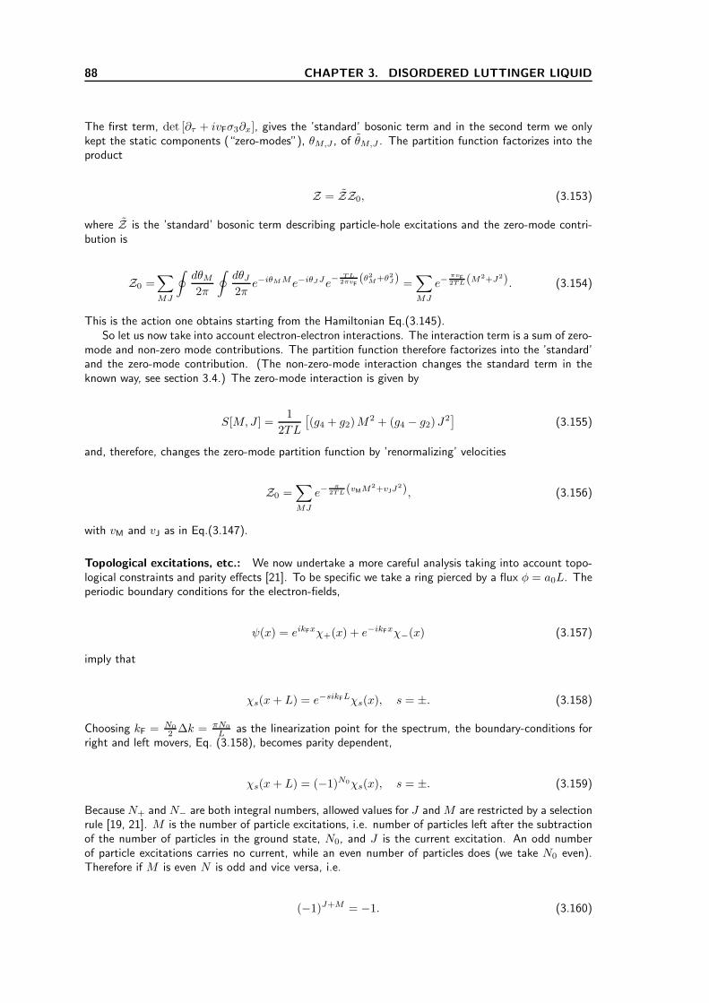
88 CHAPTER 3. DISORDERED LUTTINGER LIQUID
The first term, det [∂τ + ivFσ3∂x], gives the ’standard’ bosonic term and in the second term we onlykept the static components (“zero-modes”), θM,J , of θM,J . The partition function factorizes into theproduct
Z = ZZ0, (3.153)
where Z is the ’standard’ bosonic term describing particle-hole excitations and the zero-mode contri-bution is
Z0 =∑
MJ
∮dθM2π
∮dθJ2π
e−iθMMe−iθJJe− T L
2πvF(θ2M+θ2J) =
∑
MJ
e−πvF2T L(M2+J2). (3.154)
This is the action one obtains starting from the Hamiltonian Eq.(3.145).So let us now take into account electron-electron interactions. The interaction term is a sum of zero-
mode and non-zero mode contributions. The partition function therefore factorizes into the ’standard’and the zero-mode contribution. (The non-zero-mode interaction changes the standard term in theknown way, see section 3.4.) The zero-mode interaction is given by
S[M,J ] =1
2TL
[(g4 + g2)M
2 + (g4 − g2)J2]
(3.155)
and, therefore, changes the zero-mode partition function by ’renormalizing’ velocities
Z0 =∑
MJ
e−π
2T L(vMM2+vJJ
2), (3.156)
with vM and vJ as in Eq.(3.147).
Topological excitations, etc.: We now undertake a more careful analysis taking into account topo-logical constraints and parity effects [21]. To be specific we take a ring pierced by a flux φ = a0L. Theperiodic boundary conditions for the electron-fields,
ψ(x) = eikFxχ+(x) + e−ikFxχ−(x) (3.157)
imply that
χs(x+ L) = e−sikFLχs(x), s = ±. (3.158)
Choosing kF = N0
2 ∆k = πN0
L as the linearization point for the spectrum, the boundary-conditions forright and left movers, Eq. (3.158), becomes parity dependent,
χs(x+ L) = (−1)N0χs(x), s = ±. (3.159)
Because N+ and N− are both integral numbers, allowed values for J and M are restricted by a selectionrule [19, 21]. M is the number of particle excitations, i.e. number of particles left after the subtractionof the number of particles in the ground state, N0, and J is the current excitation. An odd numberof particle excitations carries no current, while an even number of particles does (we take N0 even).Therefore if M is even N is odd and vice versa, i.e.
(−1)J+M = −1. (3.160)

3.7. AN APPLICATION: PERSISTENT CURRENT IN A LUTTINGER LIQUID 89
This holds for periodic boundary conditions. We may account for the boundary condition, Eq. (3.158),by adding half of an elementary flux to the physical flux piercing the ring in the case of odd particlenumbers N0, i.e.
φ→ φ = φ+(1 − (−1)N0
) φ0
4, (3.161)
where φ0 = 2πe . One may equally incorporate the anti-periodic boundary conditions by demanding that
instead of selection rule, Eq. (3.160), M and J have to fulfil the condition (−1)J+M = −(−1)N0 (seebelow).
The external magnetic field (belonging to the flux piercing the ring) shifts the momenta accordingto p→ p+ ea. Therefore the kinetic energy becomes
1
2m(p+ ea)
2ψψ → 1
2m
[
2pF (q + ea) χσ3χ+ (ea)2N0
]
=vF (q + ea) χσ3χ+vFL
2π(ea)
2
=vF
(
q +2π
L
φ
φ0
)
χσ3χ+vFL
2π
(2π
L
φ
φ0
)2
, (3.162)
where we linearized around kF = πN0
L and employed that ea = 2πL
φφ0
. The magnetic flux, Eq. (3.161),therefore shifts the ’chemical potential’ θJ according to
θJ → θJ,φ = θJ +i2πvF
TL
φ
φ0. (3.163)
Following the steps of the last paragraph we end up with
Z0 =∑
MJ
∮dθM2π
∮dθJ2π
e−iθMMe−iθJJe− TL
2πvF(θ2M+θ2
J,φ)− 2πvFT L
“
φφ0
”2
, (3.164)
where the sum over M,J is restricted to fulfill the selection rule of Eq. (3.160). Using that
TL
2πvFθ2J,φ +
2πvF
TL
(φ
φ0
)2
=TL
2πvFθ2J + i2θJ
φ
φ0(3.165)
we obtain
Z0 =∑
MJ
∮dθM2π
∮dθJ2π
e−iθMMe−iθJ
“
J+ 2φφ0
”
e− T L
2πvF(θ2M+θ2J). (3.166)
Notice that the flux simply fixes the current J to
δ(J − J) → δ(J − J − 2φ/φ0). (3.167)
That is in the ground state, J = 0 (J = 1), the current is shifted due to the presence of the magneticflux, i.e. 〈J〉 = 2φ/φ0 (〈J〉 = 1 + 2φ/φ0). Adding the zero-mode interaction (notice that we haveto substitute (g4 − g2)J
2 → (g4 − g2)(J − 2φ/φ0)2) and performing the integral over the chemical
potentials we obtain
Z0 =∑
MJ
e− π
2T L
„
vMM2+vJ
“
J+ 2φφ0
”2«
. (3.168)

90 CHAPTER 3. DISORDERED LUTTINGER LIQUID
In order to compare the result, Eq. (3.168), with that obtained by D. Loss [21] we write the sums overintegers M and J as sums over even integers and ’topological excitations’ κM , κJ = 0, 1 i.e.
Z0 =∑
κM ,κJ=0,1
∑
MJ
e−πvM2T L (2M+κM )2e
−πT L2vJ
J2+i2πiJ“
κJ2 +
[N0]22 + φ
φ0
”
, (3.169)
where we performed a Poisson summation over J and [...]2 ≡ mod2(...) (we used that expiπJ(1 + (−1)N0
=
exp iπJ [N0]2). The summation over the topological excitations has to be done with the constraint(−1)κM+κJ = −1. We may therefore write
Z0 =∑
κM ,κJ=0,1
∑
MJ
e−πvM2T L (2M+κM )2e
−πTL2vJ
J2+i2πJ“
κJ2 + φ
φ0
”
, (3.170)
with κM = κJ if N0 is odd and κJ = [κM + 1]2 if N0 is even. Using further that κ2M = κM one may
equally write
Z0 =∑
κM ,κJ=0,1
∑
MJ
e−πvM2T LκM e−
2πvMT L M2
e−2πvMT L MκM e
−πT L2vJ
J2
ei2πJ
“
φφ0
+κJ2
”
=∑
κM ,κJ=0,1
∑
MJ
e−πv∗K∗
T L κM e−4πv∗K∗
T L M2
e−4πv∗K∗
T L MκM e−πT LK∗
v∗ J2
ei2πJ
“
φφ0
+κJ2
”
=∑
κM ,κJ=0,1
e−πv∗K∗
T L κM θ3(κM , zM )θ3(κJ , zJ), (3.171)
where in the second line K∗v∗ = vM
2 , v∗
K∗ = 2vJ and in the last line θ3(q, z) =∑
n qn2
ei2nz is the
Jacobi θ function and zJ = πθ02 , qJ = e−πTLK
∗/v∗ , zM = i2πκMK∗v∗/(TL), qM = e−4πK∗v∗/(TL)
and θ0 = κJ+ 2φφ0
. This equals Eq. (13) of [21]. (Notice that instead of taking into account anti-periodic
boundary conditions by working with Eq. (3.160) and adding half a flux quantum we could have equallyworked with the selection rule (−1)M+J = −(−1)N0.)
The persistent current is obtained from the free energy, F = T lnZ, according to
j = −∂φF. (3.172)
Using Eq.(3.171) one obtains [21],
j =2πT
φ0
∞∑
n=1
(−1)nN0
sin[
2πnφφ0
]
sinh[nπTLK∗
v∗F
] , (3.173)
which oscillates with a period of an elementary flux quantum, φ0 = h/e. The amplitude of thecurrent decreases exponentially with increasing size and temperature and decreasing (renormalized)Fermi velocity. Notice also that j is diamagnetic for odd N0 and paramagnetic for even N0. In the nextsubsection we show that in single channel disordered wires one finds persistent currents oscillating withhalf period, h/2e.
3.7.2 Persistent current in a weakly disordered Luttinger liquid
We now turn to the Luttinger liquid in a weakly disordered ring. In this section we assume weak disorderand apply a grand-canonical calculation. To be precise we consider the action,
S = S0[χ] + Sσ[T ] + Sbs[T, φ], (3.174)

3.7. AN APPLICATION: PERSISTENT CURRENT IN A LUTTINGER LIQUID 91
where
S0[χ] =1
2g2
∑
m,q
χm(q)[(vFq)
2 + ω2m
]χ−m(−q) (3.175)
Sσ[T ] = −1
4
∑
nm,q
trΛnT
−1nn+m(q)Πσ
m(q)Tn+mn(−q)
(3.176)
Sbs[T, χ] = − vF
8l1
∫
d2x trQ+e
iχQ−e−iχ . (3.177)
Here Q± = T±ΛT−1± , S[χ] is the Coulomb-field propagator to lowest order in g2 and we assume a
mean free path of the order of the ring length, i.e. l1 ∼ L.The following considerations are analogous to those made by Gornyi et al. in the context of WL
[5, 6]: We begin by identifying the leading contribution to the persistent current in the regime of strongdephasing, τϕvF/l1 ≪ 1. This regime takes place at sufficiently high temperatures (the precise conditionis given below). Contributions to the persistent current result from electron and hole paths encirclingthe ring at least once and in opposite direction. We can organize all these paths by the number ofbackscattering events. In the absence of interactions, all order scattering processes (including non-Cooperon diagrams) are equally important. In the presence of interactions however, long paths aresuppressed due to dephasing. In the regime of strong dephasing, τϕvF/l1 ≪ 1, the shortest path (i.e.the one containing the minimal number of backscattering processes) gives the leading contribution. Allhigher orders backscattering processes only give subleading corrections through a systematic expansionin powers of the small parameter τϕvF/l1[5, 6]. Up to here we only repeated the argument of Gornyi et
al. In difference to the WL situation, where the minimal loop contains three backscattering processes,in the ring geometry the minimal loop contains only one backscattering process. (Notice that diagramswith no backscattering process due not contribute due to charge neutrality). Technically we thereforemay expand the Q-fields to quadratic order in the generators and perform a perturbative expansion inthe backscattering term. The leading contribution results from one contraction in the backscatteringaction (see below).
Expansion in generators: Expansion in the generators to quadratic order (Gaussian approximation)gives the Cooperon propagator
S0σ[Cfb
s Cbfs ] =
1
2
∑
n(n+m)<0
∑
q
tr
Cfb,snn+m(q) [|ωm| + isvFq sgn(m)] Cbf,s
n+mn(−q)
. (3.178)
The back-scattering term in Gaussian approximation is given by Sbs[T, χ] = S1χ[χ] + Sχ[Cfb
s Cbfs ] +
Sbs[Cfbs Cbf
−s], where
S1χ =
vF
4l1
∫
d2x trΛeiχΛe−iχ
(3.179)
Sχ[Cfbs Cbf
s ] =vF
2l1
∫
d2x tr
Cfbs Cbf
s Λeiχf
Λe−iχf
(3.180)
Sbs[Cfbs Cbf
−s] =vF
4l1
∫
d2x tr
Cfb+Λeiχ
bCbf−Λe−iχ
f
. (3.181)
We regularize S1χ by subtracting a constant (T here denotes the temperature),
S1χ =
vF
4l1
∫
d2x trΛeiχΛe−iχ − T
(3.182)
=vF
4πl1
∑
m
∫
dx|ωm|(
e−iχ(x))
−m
(
e−iχ(x))
m, (3.183)

92 CHAPTER 3. DISORDERED LUTTINGER LIQUID
and keep S1χ to quadratic order in χ, i.e.
S1χ =
vF
4πl1
∑
m,q
χ−m(q)|ωm|χm(−q) =1
2g2
∑
m,q
χ−m(q)κ|ωm|χm(−q), (3.184)
where we introduced for later convenience κ = g2vF
2πl1. Eq.(3.184) describes the lowest order disorder
corrections to the RPA screening as discussed in section 3.6.1.
Sχ[Cfbs Cbf
s ] changes the Gaussian propagator, S0σ, of the right- (left-) moving particle-hole excitations.
The high-energy Coulomb interaction processes (contained in the virtual fluctuations of the Coulombfield χ) renormalize the backscattering length, as discusses in section 3.6.2. Eq.(3.180) would beof further interest if it also described dephasing. However, this is not the case as may be seen bythe following observation: Dephasing occurs due to real inelastic scattering processes, which in theKeldysh formalism is described by a classical interaction field (see Chapter 1, Current-Echoes in Metals
and Semiconductors) and is given by a diagonal matrix in Keldysh-space. Using further that in the
Keldysh formalism (see also Chapter 1) Λǫ =
(1 2Fǫ
−1
)
and CCΛ =
(CC ∗
CC
)
, where ∗ is some
non-vanishing combinations of the thermal function F and the matrices C, C, one may check, thata classical Coulomb field χ simply drops out of Eq.(3.180). That is, the Coulomb-field entering inEq.(3.180) describes only high energy interaction processes (as in the Keldysh formalism containedwithin the quantum components of the Coulomb field χ ) and therefore no dephasing. In the calculationsfor the persistent current we may therefore simply take
Sχ[Cfbs Cbf
s ] =vF
2leff
∫
d2x trCfbs Cbf
s
, s = ±, (3.185)
where leff denotes the interaction renormalized back-scattering length. The statement that Eq.(3.180)contains only interaction processes with high energy transfers is confirmed within the Matsubara form-alism by analytical calculation in Appendix B.8.
We may now calculate corrections to the free energy, F , arising from back-scattering processes. Tofirst order back-scattering,
∆F =vFT
2l1
∑
nn′,q
〈tr
Cfb+Λeiχ
bCbf−Λe−iχ
f
〉Sχ,Sσ + (+ ↔ −) , (3.186)
where 〈...〉Sχ,Sσ is the average with respect to the Coulombfield propagator the Cooperon propagatorSχ = S0
χ + S1χ and Sσ = S0
σ + Sχ. Performing the contraction in the Cooperon gives
∆F =4vFT
πl1L
∑
qq′
∑
m>0
ω2m
(ivFq + ωm + vFl−1eff )(ivFq − ωm − vFl
−1eff )
〈(eiχ)
−m,−q′(e−iχ
)
m,q′〉Sχ , (3.187)
Perturbation theory: In a first approximation we introduce a phenomenological dephasing time τϕ ≪l−11 , l−1
eff into the Cooperon propagator and treat the interaction term to lowest order in g2, i.e. (in lowestorder g2: Sχ = S0
χ),
T
L
∑
q′
〈(eiχ)
−m,q′(e−iχ
)
m,−q′〉Sχ
=T
L
∑
q′
〈χ−m(q′)χm(q′)〉S0χ
=T
L
∑
q′
g2(vFq′)2 + ω2
m
=g2T
2vF|ωm| , (3.188)
and therefore

3.7. AN APPLICATION: PERSISTENT CURRENT IN A LUTTINGER LIQUID 93
∆F =2g2T
πl1
∑
q
∑
m>0
ωm
(ivFq + ωm + vFl−1eff + τ−1
ϕ )(ivFq − ωm − vFl−1eff − τ−1
ϕ )
=2g2T
πl1
1
i4πT
∫
dΩ∑
q
−iΩ coth[
Ω2T
]
(vFq + Ω + iτ−1ϕ )(vFq − Ω − iτ−1
ϕ ).
Notice that in the first line we introduced the phenomenological dephasing rate, 1/τϕ, and in thesecond line we neglected vF/leff ≪ 1/τϕ. In a next step we perform a Poisson-summation over discretemomenta and (taking into account only the magnetic flux-dependent contributions, see Appendix B.8)obtain
∆F =g2iπl1
∑
m>0
cos [2πmx] e−2πmγ
∫
dyy coth
[y2θ
]ei2πmy
y + iγ, (3.189)
where we introduced y = L2πvF
Ω, x = 2φφ0
, γ = L2πvFτϕ
and θ = TL2πvF
. Performing the integral over y
(see Appendix B.8) we find
∆F =g2TL
πl1vF
∑
m>0
cos [2πmx] e− 2πmT L
vF e− mL
vFτϕ
sinh[
2πmTLvF
] +O(1/T τϕ). (3.190)
This leads to the persistent current
j =4g2T tbl1φ0
∑
m>0
m sin [4πmφ/φ0] e−2πmTtbe
−mtbτϕ
sinh [2πmTtb]+O(1/T τϕ), (3.191)
where we introduced the time tb = L/vF an electron needs to ballistically encircle the ring once. Thepersistent current oscillates as a function of the magnetic flux with a period of half of the elementary fluxquantum and an amplitude, which is a factor g2L/(πvFl1) smaller than in the clean case. The amplitudedecreases exponentially with increasing ring length and temperature. Higher order scattering processesare suppressed by factors τϕvF/l1 as is the case for the weak localization corrections to the Drudeconductivity, discussed in section 3.5.2. Dephasing leads to an exponential damping, j ∝ e−mtD/τϕ ,where mtb is the time an electrons needs to (ballistically) transverse the ring m times. For a comparisonwith multi-channel rings we state that in the weakly disordered quasi-1d system [22] (we reintroducethe electron’s charge e)
j =e2/Cφ0
1 + e2/(∆C)
∑
m>0
sin
[4πmφ
φ0
]
e−√
2πTmtDe−m
q
tDτϕ
(
m2T tD +m√
2πT tD
)
(3.192)
where tD = L2
D is the time an electron needs to diffusively encircle the ring once ∆ is the mean DOSat the Fermi energy and e2/C is the charging energy of the system e2/2C ∼ vF/L. The amplitude
e2/C1+e2/(∆C) results from an RPA approximation and the dephasing rate 1/τϕ is phenomenological intro-
duced.
Higher orders – Renormalization of disorder, current-amplitude and dephasing: We are nowmore ambitious and try to identify the impact from different energy regimes of the Coulomb interactionon the persistent current. Moreover we want to identify the dephasing rate caused due to electron-electron interactions. We start out from
∆F =4vFT
πl1L
∑
qq′
∑
m>0
ω2m
(ivFq + ωm + vFl−1eff )(ivFq − ωm − vFl
−1eff )
〈(eiχ)
−m,−q′(e−iχ
)
m,q′〉Sχ , (3.193)

94 CHAPTER 3. DISORDERED LUTTINGER LIQUID
which we may write as
∆F =4vFT
πl1
∫ 1/T
0
dτ∑
q
∑
m>0
ω2me
iωmτ−S(τ)
(ivFq + ωm + vFl−1eff )(ivFq − ωm − vFl
−1eff )
, (3.194)
where
S(τ) =T
2L
∑
mq
〈χ−m(q)χm(−q)〉Sχ(1 − cos [ωmτ ]). (3.195)
Performing the Poisson summation (as in the last subsection) we find (notice that latter on we takeτ = ±it+ const. and therefore the y-integral is convergent)
∆F =4vF
il1tb
∑
m>0
cos [2πmx]
∫ 1/T
0
dτe−S(τ)e−2πmγ
∫
dy−iy2e
− 2πτtbycoth
[y2θ
]ei2πmy
y + iγ, (3.196)
where we introduced y = L2πvF
Ω, x = 2φφ0
, γ = L2πvFτϕ
and θ = TL2πvF
. Rewriting
∆F =−4vF
l1tb
∑
m>0
cos [2πmx]
∫ 1/T
0
dτe−S(τ) tb2πdτe
−2πmγ
∫
dyy coth
[y2θ
]e(i2πm− 2πτ
tb)y
y + iγ, (3.197)
we may use again the result from the last subsection and obtain
∆F =−2iTL
πl1
∑
m>0
cos [2πmx] e−mLl1
∫ 1/T
0
dτe−S(τ)dτe−2π(m+i τ
tb)Ttb
sinh[
2π(m+ i τtb )T tb
] +O(vF/T l1)
=2T 2L
l1
∑
m>0
cos [2πmx] e−mL
l1
∫ 1/T
0
dτe−S(τ) 1
sinh2[
2π(m+ i τtb )T tb
] +O(vF/T l1). (3.198)
In Appendix B.8 we show that S(τ) is given by a sum of four terms, each one resulting from a differentrange of energies of the Coulomb interaction,
S(τ) = S1(τ) + S2(τ) + S3(τ) + S4(τ), (3.199)
where (κ = g2vF
2πl1)
S1(τ) =g2
2πvFln
[Λ
T
]
from energies 1/τ < |Ω| < Λ, (3.200)
S2(τ) =g2
2πvFln [sin [2πTτ + i0]] from energies κ < |Ω| < 1/τ, (3.201)
S3(τ) = −g2κ8vF
|τ | from energies T < |Ω| ≪ 1/τ, (3.202)
S4(τ) =g2κ
8vFTτ2 from energies |Ω| ≪ T , (3.203)
and therefore (up to O(vF/T l1))
∆F =2T 2L1
l1
(Λ
T
) g22πvF ∑
m>0
cos [2πmx] e−mLl1
∫ 1/T
0
dτ (sin [2πTτ + i0])g2
2πvFe
g2κ8vF
(Tτ2−|τ |)
sinh2[
2π(m+ i τtb )T tb
] .
(3.204)
This may be interpreted as follows:

3.7. AN APPLICATION: PERSISTENT CURRENT IN A LUTTINGER LIQUID 95
• Pm(τ) = 1
sinh2h
2π(m+i τtb
)Ttb
i is the probability that a particle-hole excitations encircles the ring
m times within the time iτ (to be analytically continued). Pm(τ) has double poles in the upperhalf plane (m > 0) at the value τm = imtb.
• 1l1
(ΛT
) g22πvF describes the renormalization of the back-scattering length due to virtual particle-hole
excitations (as discussed in section 1.6.2) and described by S1.
• A(τ) = (sin [2πTτ + i0])g2
2πvF determines the amplitude of the persistent current (see below).A(τ) results from S2. To lowest order in g2 we may approximate
A(τ) = A−(τ) +A+(τ) =(1 − e−i4πTτ−0
) g24πvF +
(1 − e+i4πTτ−0
) g24πvF .
A±(τ) has a branch cut due to the branch cut of the logarithm ln[1 − e±i4πTτ−0
]. Notice that
A+(τ) can be analytically continued to values of τ from the upper half plane and A−(τ) to valuesof τ from the lower half-plane.
• e− g2κ
8vF|τ |
gives corrections O(g2) to the amplitude and is irrelevant in the following
• eg2κ8vF
Tτ2
suppresses the “long-time” probability for particle hole excitations, i.e. leads to a damp-ing of the particle-hole life-time (dephasing). This term results from interactions involving lowenergies, S4.
Im
A+
A−
Pm
Re
Figure 3.3: Analytical structure of the terms Pm(τ) and A±(τ) discussed above. Pm has a single poleat τm = imtb corresponding to the classical time an electron needs to encircle the ring m times. A±have branch cuts from the logarithms.
Fig. 3.3 summarizes the analytical properties of the terms discussed. With these information on theanalycity of the various terms we may now perform the τ -integral (depicted in Fig. 3.4)
I±m =
∫ 1/T
0
dτA±(τ)e
g2κ8vF
(Tτ2−|τ |)
sinh2[
2π(m+ i τtb )T tb
] (3.205)
Let us start our discussion with I−: First we deform the τ -integration from the real axis to thecomplex half plane. As I− has a branch cut at positive complex values this is done to the negativehalf plane, see Fig. 3.5. To be precise, we change from the integral along τ ∈ [+0, 1/T ] to an integralalong the axis τ = it + 0 and τ = it + 1/T − 0 with t ∈ [0,−∞]. Next we use the periodicity ofS(τ) in order to exchange the contour parametrized by τ = it+ 1/T − 0 to a contour parametrized byτ = it− 0 (see again Fig. 3.5). These contours exactly cancel and therefore I− = 0.
Turning to I+ we proceed in the same manner, i.e. we deform the τ -integration from the real axisto the complex half plane. This is done to the positive half plane as I+ has a branch cut in the negativehalf plane, see Fig. 3.6. To be precise, we change from the integral along τ ∈ [+0, 1/T ] to an integralalong the axis τ = it+ 0 and τ = it+ 1/T − 0 with t ∈ [0,∞]. Now we use again the periodicity of

96 CHAPTER 3. DISORDERED LUTTINGER LIQUID
+0 Re
Im
1/T
Figure 3.4: Original contour of integration, which is deformed as described below.
+0Re
Im
1/T+0 Re
Im
1/T+0Re
Im
1/T
Figure 3.5: Deformation of the integration contour used to evaluate I− and discussed in the text.
S(τ) in order to exchange the contour parametrized by τ = it+ 1/T − 0 to a contour parametrized byτ = it− 0. These contours exactly cancel everywhere, apart from the region where Pm(τ = it) has itspole, i.e. at t = mtb. Evaluating I+ at the double pole, we obtain
I+m =
∫ 1/T
0
dτA+(τ)e− g2κ
8vF(Tt2−it)
sinh2[
2π(m+ i τtb )T tb
] =2π
(2πT )2
(
dte− g2κ
8vF(Tt2−it)
(1 − e−4πTt)−g24πvF
)
t=mtb
. (3.206)
Notice that in the non-interacting case g2 = 0, where A± = 1 the τ -integral vanishes, since onecan always choose the contour in the negative half-plane. Indeed on would expect that ∆F = 0 inthe non-interacting case, since the persistent current is induced by density fluctuations due to theinteraction.
+0Re
Im
1/T+0Re
Im
1/T+0 Re
Im
1/T
Figure 3.6: Deformation of the integration contour used to evaluate I+ and discussed in the text.

3.7. AN APPLICATION: PERSISTENT CURRENT IN A LUTTINGER LIQUID 97
The leading order contribution to I+ in g2 is given by
I+m =
g22πvFT
e−4πmtbT e− g2κT
8vF(mtb)
2
1 − e−4πmtbT, (3.207)
and therefore
∆F =g2T tbπ
1
l1
(Λ
T
) g22πvF ∑
m>0
cos [2πmx]e−
mLl1 e−2πmtbT e
− g2κ8vF
(mtb)2
sinh [2πmtbT ]+O(vF/T l1). (3.208)
This is what we obtained from the perturbative calculation, however with a renormalized backscatteringlength and the dephasing rate due to the electron-electron interactions
1
τpcϕ
=g22Tmtb
16πl1vF. (3.209)
This dephasing rate is in fact what one would expect [23] by the following argument:In section 3.4.2 we discussed the inelastic scattering rate in the clean Luttinger liquid and found
that it is given by
1
τee∝∫
dq
∫
dΩδ(q + Ω)δ(q − Ω). (3.210)
Technically, the dephasing rate differs from the inelastic scattering rate in the fact that the Ω-integral iscut-off by some inverse time-scale. This is due to the fact, that very-low frequency interaction processes,corresponding to time-scales exceeding the typical traveling-time of the Cooperon do not contribute todephasing as these correspond to static processes from the Cooperon’s point of view (see also Chapter2, Dephasing by Kondo impurities). Introducing such a frequency cut-off 1/ttyp one finds that thedephasing rate vanishes for the clean Luttinger liquid (see also [5, 6]). In fact we found above that thedephasing rate arises from interaction processes described by S4 which involves corrections to the RPAscreening due to disorder (i.e. which is proportional to κ).
Introducing disorder softens the δ-functions in Eq.(3.211) and leads to
1
τϕ(ttyp)∝∫
dq
∫
1/ttyp<|Ω|dΩδl1(q + Ω)δl1(q − Ω) ∝ g2
l1vFT ttyp, (3.211)
where δl1(x) = −iπ Im 1x+i/l1
. The typical traveling time for the electron-hole excitation (making up
the Cooperon) in the context of weak localization corrections to the Drude conductivity is given by thedephasing time itself. This leads to (compare Eq.(3.112))
1
τWLϕ
∝ g2
√
T
l1vF. (3.212)
T. Ludwig and A. Mirlin first observed that in the AB experiment in a diffusive wire the typical travelingtime for the Cooperon picking up a phase mφ/φ0 is given by tmtyp = mtD [23]. Correspondingly, in anearly clean wire the typical traveling time of the Cooperon picking up the phase mφ/φ0 is given bythe ballistic time tmtyp = mtb. Therefore one would, indeed, expect
1
τpc,mϕ
∝ g22Tmtbl1vF
. (3.213)
Finally we mention, that the condition τϕvF/l1 holds for temperatures
T ≫ 16πv2F
g22tb
. (3.214)

98 CHAPTER 3. DISORDERED LUTTINGER LIQUID
3.7.3 Summary of this section
In this section we studied the persistent current in a single-channel ring. In a first subsection weproposed a method how one can obtain the known results for the persistent current in a clean Luttingerliquid within the functional (σ-model) bosonization approach. The main idea was to introduce extrafields (“chemical potentials”) which fix the constraint that the number of particles is discrete. It isknown that the persistent current for the clean Luttinger liquid oscillates as a function of the magneticflux, piercing the ring, with a period given by the elementary flux quantum. In a second subsection weshowed that the disordered Luttinger liquid establishes persistent currents oscillating as a function ofthe external magnetic flux with a period given by half of the elementary flux quantum. We also foundthat the amplitude is exponentially damped by a dephasing rate due to electron-electron interactions.
3.8 Summary and outlook
In this chapter a coupled ballistic σ-model is suggested as an low-energy field theory for the disorderedLuttinger liquid. This model may be seen as the single-channel limit of an “universal” model forthe disordered interacting electron gas. The model shows how in the absence of dephasing Andersonlocalization sets in. Moreover, it becomes very effective when it comes to the analysis of interferencephenomena; as an example we calculated (in the limit where strong dephasing impedes Andersonlocalization) the persistent current in a disordered single cannel ring with weakly interacting electrons.The model may also become useful in the localization regime. In the limit of strong localization it canbe mapped on a model for granular chains, with the grains representing localization islands. This mayserve as a starting point for the analysis of electron-electron interaction induced hopping between theseislands. As already mentioned in the introduction of this chapter, some points resemble a collection ofideas and still need to be elaborated more carefully.

Bibliography
[1] K. Efetov, Supersymmetry in disorder and Chaos (Cambridge University Press, 1997).
[2] A. M. Finkel’stein, Zh. Eksp. Teor. Fiz. 84, 168 (1983); [Sov. Phys. JETP 57, 97 (1983)]; Z. Phys.B 56, 189 (1984); A. M, Finkel’stein, Electron Liquid in Disordered Conductors, Vol. 14 of Soviet
Scientific Reviews, ed. I. M. Khalatnikov. Harwood Academic Publisher, GmbH, London, 1990.
[3] A. Kamenev and A. Andreev, Phys. Rev. B 60, 2218 (1999).
[4] H. J. Schulz, in Mesoscopic Quantum Physics, edited by E. Akkermans, G. Montambaux. J.-L.Pichard, and J. Zinn-Justin (North-Holland, Amsterdam, 1995); A. O. Gogolin, A. A. Nerseyan, andA. M. Tsvelik, Bosonization and Strongly Correlated Systems (Cambridge University, Cambridge,1998); H. J. Schulz, G. Cuniberti, and P. Pieri, in Field theories for Low-Dimensional Condensed
Matter Systems, edited by G. Morandi, P. Sodano, P. Tagliacozzo, and V. Tognetti (Springer, Berlin,2000); T.Giamarchi, Quantum Physics in One Dimension (Oxfford University Press, Oxford, 2004).
[5] I. V. Gornyi, A. D. Mirlin and D. G. Polyakov, Phys. Rev. Lett. 95, 206603 (2005).
[6] I. V. Gornyi, A. D. Mirlin and D. G. Polyakov, cond-mat/0608590.
[7] C. Mora, R. Egger, and A. Altland, cond-mat/0602411.
[8] H.C.Frogedby, J. Phys. C 9, 3757 (1976); D.K.K.Lee and Y.Chen, J. Phys. A 21, 4155 (1988);I.V.Yurkevich, in Strongly correlated fermions and bosons in low-dimensional disordered systems,edited by I.V.Lerner, B.L.Altshuler, and V.I.Falko (Kluwer, Dordrecht, 2002), cond-mat/0606387;I.V.Lerner and I.V.Yurkevich, in Impurity in the Tomonaga-Luttinger model: a functional integral
approach,, to be published in Proc. LXXXI Les Houches School on Nanoscopic Quantum Transport,2004, cond-mat/0508223.
[9] J. Meyer private communication.
[10] J. Solyom, Adv Phys. bf 28, 201 (1979); J. Voit, Rep. Prog. Phys 57, 977 (1994); T.Giamarchi,Quantum Physics in One Dimension (Oxfford University Press, Oxford, 2004).
[11] A. V. Andreev, O. Agam, B. D. Simons, and B. L. Altshuler, Phys. Rev. Lett. 76, 3947 (1996);A. V. Andreev, B. D. Simons, O. Agam, and B. L. Altshuler, Nucl. Phys. B 482, 536 (1996).
[12] F. D. M. Haldane, J. Phys. C 12 (1979) 4791; J. von Delft and H. Schoeller Annalen der Physik7, 225-306 (1998).
[13] I. E. Dzyaloshinskii and K. B. Larkin, Sov. Phys. JETP 38, 202 (1973); I.V.Yurkevich,in Strongly correlated fermions and bosons in low-dimensional disordered systems, edited byI.V.Lerner, B.L.Altshuler, and V.I.Falko (Kluwer, Dordrecht, 2002), cond-mat/0606387; I.V.Lernerand I.V.Yurkevich, in Impurity in the Tomonaga-Luttinger model: a functional integral approach,to be published in Proc. LXXXI Les Houches School on Nanoscopic Quantum Transport, 2004,cond-mat/0508223.
[14] J. Zinn-Justin, Quantum Field Theory and Critical Phenomena, Oxford University Press UK (2002).
[15] R. Raimondi, P. Schwab, C. Castellani, Phys. Rev. B 60, 5818 (1999).
99

100 BIBLIOGRAPHY
[16] C. Castellani, C. Di Castro, P.A. Lee, and M. Ma, Phys. Rev. B 30, 527 (1984).
[17] I. L. Aleiner, B. L. Altshuler and M. E. Gershenson, Waves in Random Media 9, 201 (1999).
[18] A. M. Rudin, A. Aleiner, and L. I. Glazman, Phys. Rev. B 55, 9322 (1997).
[19] F. D. M. Haldane, J. Phys. C 14, 2585-2609 (1981).
[20] N. Sedlmayr, I. V. Yurkevich and I. V. Lerner, cond-mat/0607649.
[21] D. Loss, Phys. Rev. Lett. 69, 343-346 (1992).
[22] U. Eckern, Phys. Rev. Lett. 70, 3123 (1993).
[23] T. Ludwig and A. D. Mirlin, Phys. Ref. B 69, 193306 (2004).

Appendix A
Appendix (Dephasing by Kondoimpurities)
A.1 Gradient expansion
In this appendix we perform the gradient expansion to obtain the effective action given in Eqs. (2.26),(2.27) and (2.28). The gradient expansion employs the fact that Q describes the low-energy/low-momentum sector of the theory, reflected in the dependency of Q only on small momenta, Dq2τ ≪ 1,and small frequencies, ωmτ ≪ 1. Starting out from the action,
S[g] =1
2Tr ln
i∂τ +1
2m∂2 + µ+
i
2τgΛg−1 − J
∑
i
σSσT3 S(xi)
,
the strategy is to express the rotation matrices, g, in generators and to expand the “Tr ln” in thegenerators as well as the small parameters Dq2τ , ωmτ ≪ 1 and 1/ǫFτ ≪ 1, keeping all orders in J .For notational convenience we introduce the following Green’s functions
G0(p) ≡(− p2
2m+ µ+
i
2τΛ)−1
GS0 (p) ≡
(− p2
2m+ µ+
i
2τΛ − JσSσT
3 S)−1
,
where we used the short notation σSσT3 S ≡∑i σ
SσT3 S(xi). Using that the rotation matrices, g, depend
only on small momenta we decompose the momentum operator,
p 7→ p + q,
where the large momenta p enter through the global summation in the trace and the small momentum-operator q acts on the effective degree of freedom g. As already mentioned we parametrize the rotation-matrix fields g(x)ττ ′ by generators W ,
Q = gΛg−1 = e−W/2ΛeW/2 = ΛeW ,
where the second equality follows from the requirement that the Lie-algebra elements W generaterotations g that act on the saddle point fixed-point free, i.e.
[Λ,W
]= 0. We proceed by expanding g
in W and expansion of the “Tr ln” to second order in W (Gaussian approximation)
101

102 APPENDIX A. APPENDIX (DEPHASING BY KONDO IMPURITIES)
2S[g] =Tr ln∂τ + µ+
p2
2m+
i
2τgΛg−1 − JσSσT
3 S
=Tr ln∂τ + µ+
p2 + 2pq
2m− JσSσT
3 S +i
2τΛ +
i
2τΛW +
i
4τΛW 2
=Tr ln[GS
0
]−1+
pq
m+ ∂τ +
i
2τΛW +
i
4τΛW 2
=Tr ln1 + GS
0
(pq
m+ ∂τ +
i
2τΛW +
i
4τΛW 2
)
=TrGS
0
(pq
m+ ∂τ +
i
2τΛW +
i
4τΛW 2
)− 1
2
GS
0
(pq
m+ ∂τ +
i
2τΛW +
i
4τΛW 2
)2
+1
6TrGS
0
(pq
m+ ∂τ +
i
2τΛW +
i
4τΛW 2
)3 − ...
In the second line we neglected a term proportional to q2, and in the fourth and the last line we neglectedconstant contributions. Also we employed the fact that in order to find corrections to the conductivityup to order O
(1/(ǫFτ)
2)
we can rely on the Gaussian approximation, that is we only need to expandto second order in the generators W . We now want to find for each order in J the most relevantcontributions. Using that every Greens function after integration over fast momenta contributes by afactor τ (see Eq. (A.1)) (i.e. terms with higher derivatives are corrections of the order (ωmτ)
k ≪ 1and (Dq2)kτ ≪ 1, k > 0) we find for the J0-order
SJ=0[W ] =i
8τTrG0ΛW
2
+1
16τ2TrG0ΛWG0ΛW
− i
8τTrG0∂τG0ΛW
2
− 1
16τ2TrG0∂τG0ΛWG0ΛW
+
i
16τTrG0
pq
mG0
pq
mG0ΛW
2)
+ ....+ O(W 3).
We proceed by writing G0(p) = 12
(1+Λ
)Gr
0(p)+ 12
(1−Λ
)Ga
0(p), where Gr/a0 (p) =(− p2
2m+µ±i/2τ)−1
and employ the identity
∫
ddp[Gr0(p)
]k+1[Ga0(p)
]m+1= (−1)k2πνik+m
(k +mm
)
τk+m+1, (A.1)
in order to find for the J = 0 contribution,
SJ=0[W ] = S2σ[W ] = −πν
8
∑
n1n2
∫
ddqTr(Dq2 + 2ǫΛ
)Wn1n2(q)Wn2n1(−q)
.
Turning to contributions with non-vanishing J we again neglect those terms containing derivatives ∂τand q (they constitute corrections of the order ωmτ ≪ 1 and Dq2τ ≪ 1). This leaves us with thefollowing three terms
S[J 6= 0,W ] =iJ
8τTrG0σ
SσT3 SGS
0ΛW 2
+J
8τ2TrG0σ
SσT3 SGS
0ΛWG0ΛW
+J2
16τ2TrG0σ
SσT3 SGS
0ΛWG0σSσT
3 SGS0ΛW
,
where we employed that GS0 = G0 + JG0σ
SσT3 SGS
0 . Using the decomposition of G0 in retarded andadvanced components we can see that the first term vanishes, since
TrG0σ
SσT3 SGS
0ΛW 2
= const.
∫
ddpGR0 GA
0 Tr(
1 ∓ Λ)σSσT
3 S(1 + JGS
0σSσT
3 S)(
1 ± Λ)ΛW 2
= const.
∫
ddpGR0 GA
0 TrσSσT
3 S(1 + JGS
0σSσT
3 S)(
1 ± Λ)(
1 ∓ Λ)ΛW 2
,

A.2. SPIN-SINGLET AND SPIN-TRIPLET CHANNELS 103
and(1 ∓ Λ
)(1 ± Λ
)= 0. The second term, on the other hand, acquires the form
− J
8τ2Tr
G0σSGS0ΛWGS
0ΛW
= − J
16τ2
∑
p
GR0 (p)GR
0 (p)GA0 (p)Tr
(σSσT
3 S + JσSσT3 SGS
0σSσT
3 S)ΛW 2(1 + Λ)
− J
16τ2
∑
p
GR0 (p)GA
0 (p)GA0 (p)Tr
(σSσT
3 S + JσSσT3 SGS
0σSσT
3 S)ΛW 2(1 − Λ)
= − πνiJ
4Tr(σSσT
3 S + JσSσT3 SGS
0σSσT
3 S)ΛW 2
,
and the last may be written as
1
16τ2Tr
G0σSGS0ΛWG0σ
SσT3 SGS
0ΛW
=1
16τ2
∑
p′
∑
p
GR0 (p)GA
0 (p)GR0 (p′)GA
0 (p′)
Tr(σSσT
3 S + JσSσT3 SGS
0σSσT
3 S)ΛW
(σSσT
3 S + JσSσT3 SGS
0σSσT
3 S)ΛW
.
Integration over the fast momenta we find Eqs. (2.26), (2.27) and (2.28). We notice that since themagnetic impurity is a hard scatterer, i.e. incoming momenta are scattered over the whole Fermi-sphere,every Greens function between two local spins gives a term
∫ddpG0(p). That is every order in J comes
with a free integration over the Fermi-sphere and thus the k-th order in J gives a correction ∼ (JνLd)k.In the case of soft scatterers different contributions are dominant; see the evaluation of the correctionsto 1/τϕ from mixed diagrams and higher orders in nS in the text and in Appendix A.7 and A.8 for adiscussion of this point.
A.2 Spin-singlet and spin-triplet channels
In this appendix we separate the effective degrees of freedom (Diffuson and Cooperon), which describethe joined propagation of two spin-1/2 particles, into its spin-singlet and spin-triplet contributions. Tothis end we remind that the spin-singlet state is by definition the one-dimensional space on which theaction of the spin SU(2) is trivial. Introduction of a Zeeman-term allows for a further identification ofthe spin-triplet states with z-component m = −1, 0, 1.
A.2.1 Spin-singlet channels
By definition the spin SU(2) acts trivial on the spin-singlet state. For a representation of the action ofSU(2) on the Diffuson and Cooperon, respectively, we go back to the definitions,
Ψ =1√2
(ψ
−iσS2ψ
t
)
T
, Ψ =1√2
(ψ −iψtσS
2
)
T, Q ∝ Ψ ⊗ Ψ, (A.2)
and remind that the Diffuson corresponds to the T-space diagonal terms, D ∝ χ ⊗ χ. That is, theaction of the SU(2) is given by the complex adjunct representation,
χ⊗ χ→ gχ⊗ χg†, (A.3)
from which we read off the invariant singlet sub-space spanned by DS=0 = sD ⊗ σS0 . The Cooperon on
the other hand is given by the T-space off-diagonal terms, C ∝ χ⊗χtσS2 . Therefore the SU(2) acts by
the real conjugate representation,

104 APPENDIX A. APPENDIX (DEPHASING BY KONDO IMPURITIES)
χ⊗ χtσS2 → gχ⊗ χtgtσS
2 , (A.4)
which also has the one-dimensional invariant subspace CS=0 = sC ⊗ σS0 . For completeness we give
the diagrammatic representation of the Diffuson and Cooperon singlet-states in terms of advanced andretarded Greens functions.
Spin-singlet Diffuson
+ + +
Spin-singlet Cooperon
−+ −
A.2.2 Spin-triplet channels
The triplet components of Diffuson and Cooperon are spanned by the generators, W , proportionalto σS
1 , σS2 , σ
S3 . In order to find the Sz = −1, 0, 1 components we introduce a Zeeman term into the
Hamiltonian,
HZee =
∫
ddxχ(x)BzσS3χ(x), (A.5)
where Bz is a (homogeneous) external magnetic field defining the z-axis of the coordinate system.Introduction of a time-reversed component and following the steps for the derivation of the σ-modelone ends up with the following additional contribution to the σ-model action
SZee[W ] =∑
n1n2
∫
ddx trBzσ
S3σ
T3 Λn1Wn1n2Wn2n1
. (A.6)
Separation into Diffuson and Cooperon contributions one obtains
SZee[D++] =∑
n1n2
∫
ddx trBzΛn1
[σS
3 ,D++n1n2
]D++n2n1
(A.7)
SZee[C+−C−+] =∑
n1n2
∫
ddx tr
BzΛn1
[σS
3 , C+−n1n2
]
+C−+n2n1
. (A.8)
Notice that the Cooperon-singlet is not diagonal in the Zeeman term (i.e. an invariant subspace of).This results from the fact that the magnetic field in the time-reversed space comes with a minus sign.In order to distinguish the Cooperon-triplet components one may work for the Cooperon with the modelHamiltonian
SZee[WC] =
∑
n1n2
∫
ddx trBzσ
S3Λn1W
Cn1n2
WCn2n1
, (A.9)

A.2. SPIN-SINGLET AND SPIN-TRIPLET CHANNELS 105
singlet triplet m = 0 triple m = 1 triplet m = −1
Diffuson DS=0 = sD⊗σS0 DS=1,0 = tD0 ⊗σS
3 DS=1,1 = τD1 ⊗
(σS
1 + iσS2
)DS=1,−1 = τD
−1⊗(σS
1 − iσS2
)
Cooperon CS=0 = sC ⊗ σS0 CS=1,0 = tC0 ⊗ σS
3 CS=1,1 = τC1 ⊗
(σS
1 + iσS2
)CS=1,−1 = τC
−1 ⊗(σS
1 − iσS2
)
Table A.1: Separation of Diffuson and Cooperon into its spin-singlet and spin-triplet contributions.
which takes the form
SZee[C+−C−+] =∑
n1n2
∫
ddx trBzΛn1
[σS
3 , C+−n1n2
]C−+n2n1
. (A.10)
However, we only use Eq. (A.10) in order to identify the m = −1, 0, 1 triplet states. A physical B-fieldmakes the modes WC ∝ σS
3 ±σS0 massive, while WC ∝ σS
1 , σS2 are not affected. With Eqs. (A.7), (A.10)
it follows that the Sz = 0 triplet-Diffuson and -Cooperon are given by WS=1 ∝ t0 ⊗ σS3 whereas the
m = ±1 states are linear combinations of WS=1 ∝ t1 ⊗ σS1 and WS=1 ∝ t2 ⊗ σS
2 . To be more precise,the latter diagonalize the Hamiltonian, i.e.
(t1 t2
)
nn′
(Πnn′ −iBz
iBz Πnn′
)(t1t2
)
n′n
=1
2
(t1 + it2 t1 − it2
)
nn′
(Πnn′ + Bz
Πnn′ − Bz
)(t1 − it2t1 + it2
)
n′n
≡(τ1 τ2
)
nn′
(Πnn′ + Bz
Πnn′ − Bz
)(τ1τ2
)
n′n
, (A.11)
where tnn′ and tnn′ again denote contributions with n < 0, n′ > 0 and n > 0, n′ < 0 (correspondinglyfor s and τ) and Π−1
nn′ = Dq2 + iǫn−n′ is the propagator of the standard nonlinear σ-model action. Insummary, contributions from the spin-triplet channels to the action are
Sσ[t0t0] =
∫
ddq trR
Π−1 t0t0
(A.12)
Sσ[τ1τ1] =
∫
ddq trR
[Π−1 + Bz
]τ1τ1
(A.13)
Sσ[τ−1τ−1] =
∫
ddq trR
[Π−1 − Bz
]τ−1τ−1
. (A.14)
The results of this section are summarized in Table A.1 and a diagrammatic representation of the tripletstates in terms of Greens functions is depicted below.
Spin-triplet Diffusons: m = −1, 0 and 1
+ −−
Spin-triplet Cooperons: m = −1, 0 and 1
++ +

106 APPENDIX A. APPENDIX (DEPHASING BY KONDO IMPURITIES)
A.3 Response kernels in Gaussian approximation
In this appendix we derive the response kernels for the calculation of weak localization corrections to theconductivity (WL) and the Aharonov-Bohm oscillations (AB), Eqs. (2.55)-(2.56) and Eqs. (2.94)-(2.96).
We start out from the definition of the (homogeneous) dc-conductivity in a d-dimensional system
in the linear-response approximation, σ = −K(ω)iω , where
K(ωm) ≡ 1
d
d∑
i=1
δ2F [a]
δai0(ωm)δai0(−ωm)(A.15)
is the linear response kernel, a0 denotes the homogeneous component a(q = 0) of the vector potentialand the analytical continuation iωm → ω + i0 has to be done. Next we perform an expansion in thegenerators W to second order (Notice that we introduced a into the action Eq. (2.26) by minimallycoupling, i∂ 7→ i∂+e[aσT
3 , .]). In 0th order fluctuation matrices, W , the source term of action Eq. (2.26)takes the form,
S0dia[a] =
e2πνD
4traσT
3 ΛaσT3 Λ − 2aa
,
leading to (here and in the following summation over repeated indices is implicit)
Kmf(iωm) =e2πνD
βtr2n1 − Λn1(Λn1+m + Λn1−m)
,
which gives the Drude conductivity, σD. The second order contribution to the source action contains a”diamagnetic” (∝ a2) and a ”paramagnetic” (∝ a) term,
S2dia[W, a] =
e2πνD
4traσT
3 ΛW (q)aσT3 ΛW (−q) + aσT
3 ΛaσT3 ΛW (q)W (−q)
S2para[W, a] =
eπνD
2traqσT
3W (q)W (−q).
Since a is diagonal in T-space, the contributions from matrices diagonal (Diffuson) and off-diagonal(Cooperon) in T-space decouple, i.e. the source term in Gaussian approximation can be separated intoits Cooperon and Diffuson contributions. Depending on the experiment that we want to describe wekeep only one of these terms: The WL experiment involves only the Cooperon, while the AB experimentin general involves Cooperon and Diffuson degrees of freedom. Yet at already moderate magnetic fieldsthe Cooperon-contribution may be neglected.
A.3.1 Response kernel for weak localization experiment
Referring to the parametrization of Eq. (2.29), the Cooperon-contribution to the diamagnetic sourceterm is
S2dia[C+−C−+] =
e2πνD
2βam1am2 trR⊗ S
[C+−n1−m2,n2
(q) + C+−n1,n2−m2
(q)]C−+n2,n1+m1
(q)
sign [n1(n1 +m)] .
In the absence of any interactions there is only one possible contraction, resulting from
K0dia(iωm) =
e2πνD
βtrC+−n1,n2+m(q)C−+
n2n1+m(−q)
sign [n1(n1 +m)]

A.3. RESPONSE KERNELS IN GAUSSIAN APPROXIMATION 107
and leading to Eq. (2.55). In the presence of (perturbatively treated) interactions there are severalpossible ways to perform contractions between S2
dia[C] and S2int[C], i.e. we have to keep all terms in
S2dia. This leads to
Kdia(iωm) =e2πνD
βtr [
C+−n1+m,n2
(q) + C+−n1,n2+m(q)
]C−+n2n1+m(−q)
sign [n1(n1 +m1)] .
The paramagnetic contribution to the source-term action,
S2para[C+−C−+] =
eπνD
2β1/2qam1 trR⊗T
C+−n1,n2
(q)C−+n2,n1+m1
(−q)
Θ(n1(n1 +m1)),
may be expanded to second order, i.e. eSpara = 1 + Spara + 12S
2para. Performing one contractions one
finds (for a d-dimensional system)
〈S2para[C+−C−+]S2
para[C+−C−+]〉
=(eπνD)2
β
q2
dam1am2Π
Cn1n2
trR⊗T
[C+−n1−m2,n2
(q) + C+−n1,n2−m2
(q)]C−+n2,n1+m1
(−q)
Θ(n1(n1 +m1)),
i.e.
Kpara(iωm) =2(eπνD)2
β
q2
dΠCn1n2
(q) trR⊗T
[C+−n1+m,n2
(q) + C+−n1,n2+m(q)
]C−+n2,n1+m(−q)
Θ(n1(n1 +m)).
Notice that in the absence of interactions there are no possible contractions from Spara. The sum ofdiamagnetic and paramagnetic contributions may be organized as follows
Kdia(iωm) +Kpara(iωm) =e2πνD
β
[
1 + 2πνDq2
dΠCn1n2
(q)
]
Θ(n1(n1 +m)) − Θ(−n1(n1 +m))
trR⊗T
[C+−n1+m,n2
(q) + C+−n1,n2+m(q)
]C−+n2,n1+m(−q)
.
Employing that (after the contractions) the final term contains two further Cooperon-propagators, ΠC,one may write the propagator in the first line as a derivative, i.e.
Kdia(iωm) +Kpara(iωm) =e2πνD
β
[
1 + q1d
dq1
]
Θ(n1(n1 +m)) − Θ(−n1(n1 +m))
trR⊗ S
[C+−n1+m,n2
(q) + C+−n1,n2+m(q)
]B−+n2,n1+m(−q)
.
Partial integration in q1 reveals that the first contribution is exactly zero, leaving us with
Kdia(iωm)+Kpara(iωm)
= −e2πνD
βtrR⊗ S
[B+−n1+m,n2
(q) + B+−n1,n2+m(q)
]B−+n2,n1+m(−q)
Θ(−n1(n1 +m)),
which gives Eqs. (2.55) and (2.56). Notice that in the end only those terms where the current-vertexchanges causality contribute.
A.3.2 Response kernel for Aharonov-Bohm oscillations
We now turn to the AB-response kernel and restrict to the Diffuson-contribution and a (quasi)1-d
geometry. The AB are found from the typical sample-to-sample fluctuations, var g = 〈g2〉 − (〈g〉)2.Ensemble fluctuations are most conveniently computed by enlarging the internal field-space by a fluc-
tuation sector F. The vector-potential becomes a matrix in F-space, a =
(a1
a2
)
F
, and fluctuations
are obtained from

108 APPENDIX A. APPENDIX (DEPHASING BY KONDO IMPURITIES)
var g =1
L2
1
ωm1ωm2
δ4F [a]
δa1m1δa1
−m1δa2m2δa2
−m2
|iωm1 ,iωm2→i0,
where, ai is a (homogeneous) vector potential pointing along the wire. Connected diagrams con-tain only generators with off-diagonal components in F-space. Separation into dia- and paramagneticcontributions gives, S2
a = S2dia + S2
para, where
S2dia[D] =
e2πνD
2βtrR⊗ S
[am1am2D++
n1−m2,n2(q) + am1D++
n1,n2+m2(q)am2
]D++n2,n1+m1
(q)
sign [n1(n1 +m1)]
S2para[D] =
eπνD
2β1/2q trR⊗T
am1D++
n1,n2(q)D++
n2,n1+m1(−q)
Θ(n1(n1 +m1)).
Expansion to fourth order, i.e. eS2[a] = 1 + S2[a] + ..., obtains
KAB =1
2!〈S2
diaS2dia〉 +
3
3!〈S2
diaS2paraS
2para〉 +
1
4!〈S2
paraS2paraS
2paraS
2para〉.
We now perform contractions in fluctuation matrices of the paramagnetic term, in order to end up witha contribution quartic in D. To this end we use that (in d= 1)
〈S2para[D++]S2
para[D++]〉
=2(eπνD)2
β
q2
dΠDn1n2
trR⊗T
[am1am2D++
n1−m2,n2(q) − am1D++
n1,n2+m2(q)am2
]D++n2,n1+m1
(−q)
Θ(n1(n1 +m1)),
in order to organize KAB as follows
KAB =(e2πνD)2
8β2trR⊗T O[a, n1n2,m1] trR⊗T O[a, n′
1n′2,m
′1][
sign(n1(n1 +m1)) sign(n′1(n
′1 +m′
1))
+ πνDq2ΠDn1n2
Θ(n1(n1 +m1)) sign(n′1(n
′1 +m′
1)) + πνD)2q4[ΠDn1n2
]2Θ(n1(n1 +m1))Θ(n′
1(n′1 +m′
1))]
.
Here we used the short notation
trR⊗T O[a, n1n2,m1] = trR⊗T
[am1am2D++
n1−m2,n2(q) − am1D++
n1,n2+m2(q)am2
]D++n2,n1+m1
(−q).
Writing sign(n1(n1 + m1)) = Θ(n1(n1 + m1)) − Θ(−n1(n1 + m1)) one can verify that the termproportional to Θ(n1(n1 + m1))Θ(−n′
1(n′1 + m′
1)) does not give any contributions when doing thecontractions in D and therefore
KAB =(e2πνD)2
8β2trR⊗T O[a, n1n2,m1] trR⊗T O[a, n′
1n′2,m
′1]
[
Θ(−n1(n1 +m1))Θ(−n′1(n
′1 +m′
1)) +(
1 + (πνD)2q4[ΠDn1n2
]2Θ(n1(n1 +m1))Θ(n′
1(n′1 +m′
1))) ]
.
Again, we employ that the final expression contains two more Diffuson-propagators in order to write ΠD
as a derivative. Doing partial integrations it may then be seen that, again, only those terms survive,where causality is changed at the current vertex, i.e.
KAB =(e2πνD)2
β2trR⊗T O[a, n1n2,m1] trR⊗T O[a, n′
1n′2,m
′1]Θ(−n1(n1 +m1))Θ(−n′
1(n′1 +m′
1)).

A.4. SOME DETAILS 109
Performing the derivative with respect to ai we find var g = Kν + KD, where (1,2 denotes F-spacecomponents)
Kν =(e2πνD)2
β2L2ωm1ωm2
∑
−m1<n1<0
∑
−m2<n2<0
trR⊗ S
C12n1+m2,n2
(q)C21n2,n1+m1
(−q)
trR⊗ S
C12n′
1+m′2,n
′2(q)C21
n′2,n
′1+m′
1(−q)
KD =(e2πνD)2
β2L2ωm1ωm2
∑
−m1<n1<0
∑
−m2<n2<0
trR⊗ S
C12n1,n2+m2
(q)C21n2,n1+m1
(−q)
trR⊗ S
C12n′
1,n′2+m
′2(q)C21
n′2,n
′1+m′
1(−q)
.
The first and second term describe ensemble fluctuations of the density of states, ν, and the diffusionconstant, D, respectively [22]. (For notational convenience we did not write out the T-space indices+/−.)
A.4 Some details
In this appendix we show that Id(Ω, τϕ) ∼ [Ω2 + 1/τ2ϕ]
d−44 . Using that
Id(Ω, τϕ) =
∫
ddq1
(Dq2 + 1/τϕ)2 + Ω2=
1
Dd/2ΩIm
∫
ddq1
q2 + 1/τϕ − iΩ(A.16)
one finds up to orders O(
Ω2
1/τ2ϕ+Ω2
)
• in d = 1
I1(Ω, τϕ) =2π
D1/2ΩIm
1√
1/τϕ − iΩ∼ π
D1/2
1
(1/τ2ϕ + Ω2)3/4
(A.17)
• in d = 2
I2(Ω, τϕ) =−πDΩ
Im ln[1/τϕ − iΩ] ∼ π
D
1
(1/τ2ϕ + Ω2)1/2
(A.18)
• in d = 3
I3(Ω, τϕ) =−8π2
D3/2ΩIm√
1/τϕ − iΩ ∼ 4π2
D3/2
1
(1/τ2ϕ + Ω2)1/4
(A.19)
Here we used in d = 1 (and similar in d = 3) that
Im1
√
1/τϕ − iΩ=
1
(1/τ2ϕ + Ω2)1/4
Im ei/2 arcsin Ω√
1/τ2ϕ+Ω2
.
Furthermore we employed that sinx = sin 2x2 cosx and |Ω/
√
1/τ2ϕ + Ω2| < 1 in order to approximate
Im1
√
1/τϕ − iΩ=
Ω
(1/τ2ϕ + Ω2)3/4
1
2 cos 12 arcsin Ω√
1/τ2ϕ+Ω2
=Ω
2(1/τ2ϕ + Ω2)3/4
(
1 +O
(Ω2
1/τ2ϕ + Ω2
))
.
In d = 2 we approximated
arcsinΩ
√
1/τ2ϕ + Ω2
=Ω
√
1/τ2ϕ + Ω2
(
1 +O
(Ω2
1/τ2ϕ + Ω2
))
.
Taking into account the higher orders gives only corrections of numerical factors but no parametrical dif-ferent results in the estimate of the inelastic vertex contributions (notice e.g. that 1
cos 12 arcsin Ω√
1/τ2ϕ+Ω2
<
√2).

110 APPENDIX A. APPENDIX (DEPHASING BY KONDO IMPURITIES)
A.5 Some more details
In this appendix we want to show that assuming that the inelastic vertex, Γin(Ω) is a peaked functionof width ∆E the correction to the WL due to inelastic processes is given by
∆σ2
∆σWL∼ max
(1
∆Eτϕ
)(4−d)/2,
1
∆Eτϕ
(A.20)
This may be seen as follows: We showed that the first order corrections from the vertex take the form
∆σ2 =
∫
dǫ
∫
dΩf(ǫ,Ω)Γ(ǫ,Ω)Id(Ω). (A.21)
We write the vertex as a sum of its elastic and inelastic part, Γ = Γel + Γin and approximate the elasticpart by Γel(Ω) = Ω
τϕδ(Ω), such that
∆σel =
∫
dǫ
∫
dΩf(ǫ,Ω)Γel(ǫ,Ω)Id(Ω) =
∫
dΩ1
τϕId(Ω)δ(Ω) ∼ τ (2−d)/2
ϕ ∼ ∆σWL (A.22)
Assuming that Γin is a peaked function in Ω of width ∆E, we may approximate it by Γin(Ω) =Ωτϕ
∆EΩ2+∆E2 . Then we can use that for any integer m > 0
∫dΩ
2π
1
(Ω2 + 1/τ2ϕ)m
∆E
Ω2 + ∆E2∼ 1
∆E
(1
1/τ2ϕ + ∆E2
)m
+τ2m−1ϕ
τ2ϕ + ∆E2
, (A.23)
where we further assumed that ∆Eτϕ ≫ 1 and kept only the leading order terms. As this holds for anyinteger m > 0, one finds (by analytical continuation)
∆σ2 =∆E
τϕ
∫
dΩ1
(1/τ2ϕ + Ω2)(4−d)/4
1
Ω2 + ∆E2
∼τ (2−d)/2ϕ
(1
(1 + (∆Eτϕ)2)(4−d)/4+
∆Eτϕ1 + (∆Eτϕ)2
)
=∆σWL max
(1
∆Eτϕ
)(4−d)/2,
1
∆Eτϕ
. (A.24)
A.6 Renormalized perturbation theory for the
Anderson model
At temperatures well below the Kondo temperature, i.e. T ≪ TK analytic calculations can be performedwithin the framework of a Fermi liquid approach based on perturbation theory for the Anderson model[19]. In the single impurity Anderson model one describes the conduction band electrons coupled tothe local magnetic moment centered at the origin by
H = Hce(c†, c) +Hd(d
†, d) +Hhyb.(c†, c, d†, d),
where Hce describes the dynamics of the conduction band electrons (see Eq. (2.1)),
Hd =∑
σ
(ǫd − µ)d†σdσ + Und↑nd↓
is the Hubbard Hamiltonian for the local impurity and

A.7. FLUCTUATIONS OF THE KONDO-TEMPERATURE 111
Hhyb. = V∑
kσ
(d†σcσ + h.c.
)
is the hybridization of the local level with the conduction band. One recovers the physics of Kondomodel in the limit of strong on-site repulsion U . The strongly interacting model can be treated withina renormalized perturbation theory [19], where the free d-electrons Greens function is given by
Gd(ǫn) = 〈d†ndn〉 =1
iǫn + iTK sgn(n),
the interaction between d-electrons takes the form
V = TKd†n+mdnd
†n′dn′+m
and the hybridization is
Hhyb. =(TK
ν
) 12∑
kσ
(d†ncn + h.c.
).
Notice that, as we are interested only in orders of magnitude we just give the relevant energy scales,neglecting factors of π or 2,... . The diagrammatic representation for the d-electron Green’s function,the hybridization and the d-electron interaction is given on the right hand side.
Effective Interactions:
V R(Ω) =nST
2K
TK − iΩ
V Rscreen.(Ω) =
n2S
ν
Dq2
Dq2 − iΩ
A.7 Fluctuations of the Kondo-temperature
We use the following defining equation for the Kondo temperature,
∫ EF
TK
dων(ω)
ω=
1
J, (A.25)
and find for its fluctuations
(δTK
TK
)2
=1
ν2
∫ EF
TK
dω
∫ EF
TK
dω′⟨δν(ω)δν(ω′)
⟩
ωω′ . (A.26)
Here ν denotes the local DOS. In order to find the effect of disorder on the Kondo temperature, wetherefore have to calculate the mesoscopic fluctuations of the local DOS. Their leading contribution isgiven by the following diagram,
∝∫(dp)GR
p GAp
∫(dp′)GR
p′GAp′
∫(dq)Π
C/Dq (ω)

112 APPENDIX A. APPENDIX (DEPHASING BY KONDO IMPURITIES)
which gives
⟨δν(ǫ+ ω)δν(ǫ)
⟩= ν Re
∫
(dq)1
Dq2 − iω. (A.27)
Evaluation of the integral in quasi-1d and d = 2, 3 gives
Re
∫
(dq)1
Dq2 − iω=
1L2
⊥
ω−1/2
D1/2 , quasi-1d1D ln[ωτ ] d = 21√τ
1D3/2 d = 3.
(A.28)
Finally, we obtain for the fluctuations of the Kondo temperature in quasi-1d and d = 3
(δTK
TK
)2
∼
1kFl
1(k2
FL⊥)2
√EF
TKquasi-1d
1(kFl)2
1(Jν)2 d = 3.
(A.29)
The case of d = 2 has to be treated with some more care and gives
(δTK
TK
)2
∼ 1
kFl
1
(Jν)3d = 2. (A.30)
These results were stated in Eq. (2.76).
A.8 Limits of applicability: Cross-over temperatures for the dephasing-rate
Restricting to low temperatures, T ≪ TK, we calculate contributions to the dephasing rate, resultingfrom different types of diagrams that were neglected in formula Eq. (2.52). These diagrams includemixed scattering processes from static and dynamic disorder and are depicted in Figs 1(a) and (b)below. In order to obtain analytically expressions we employ renormalized perturbation theory, validfor temperatures T ≪ TK, and summarized in Appendix A.6. As we are only interested in parametricdependencies of 1/τϕ we may calculate it from self-energy diagrams with 1/τϕ included self-consistentlyas the IR cut-off,
1
τϕ=
∫
τ−1ϕ
dΩΩ
T sinh2[
Ω2T
]V (Ω), (A.31)
i.e. we do not explicitly take into account the vertex contributions. Here V represents an effectiveinteraction different for each diagram.
Dephasing-rate in Fermi liquid regime: In a first step we evaluate the dephasing-rate Eq. (2.81)obtained from neglecting mixed scattering from static and dynamic disorder in the low temperatureregime T ≪ TK. The relevant diagram for the very low temperature regime is depicted in Fig. 1(a).Below we show that
V (a)(Ω) =nSΩ
νT 2K
, (A.32)
and therefore
1
τaϕ=nS
ν
( T
TK
)2
in d = 1, 2, 3. (A.33)

A.8. LIMITS OF APPLICABILITY: CROSS-OVER TEMPERATURES FOR THEDEPHASING-RATE 113
In a next step we compare result Eq. (A.33) with corrections arising from the interplay between in-teractions and scattering from static impurities. The role of correlations disorder/interactions maybe explored in terms of the diagrams shown in Fig. 1(b) and (c). On face of it, these diagrams aresmaller by factors of 1/(kFl) than the leading contributions, Eq. (A.33). This suppression results fromthe fact that quantum interference maintained across the impurity limits the momentum exchange tovalues < l−1 much smaller than kF. However, in the very low T regime, that we are considering,the enhanced infrared singularity caused by the presence of additional Diffuson/Cooperon modes mayover-compensate this phase space suppression factor.
Interplay between scattering from static and dynamical impurities – linear order in nS: Firstwe look at diagrams linear order in nS as depicted in Fig. 1(b). Below we show that
V (b)(Ω) =nS
ν2T 2K
Ω
Dd/2
Ω−1/2
(kFL⊥)2 , quasi-1d
1, d = 2
τ−1/2, d = 3
(A.34)
and therefore
1
τbϕ=
nS
ν2T 2K
1
Dd/2
T 3/2
(kFL⊥)2 quasi-1d
T 2, d = 2
T 2τ−1/2, d = 3.
(A.35)
Interplay between scattering from static and dynamical impurities – Higher order in nS: Fi-nally we account for scattering processes from different magnetic impurities. At very low T theKondo impurities become indistinguishable from a conventional disordered Fermi liquid with short-rangemomentum-conserving interactions. Therefore the dephasing-rate should be dominated by Altshuler-Aronov-Khmelnitsky [1] type processes, shown in Fig. 1(c). Although these type of processes givecorrections which contribute only at order n2
S they become important at low temperatures, since theyscale as T 2/3, T and T 3/2 in d = 1, 2, 3, respectively. More precisely, we find find from the diagrams,that
V (c)(Ω) =n2
S
ν3T 2K
Ωd/2−1
Dd/2
1
(kFL⊥)2 , quasi-1d
1 d=2,3,(A.36)
which results in
1
τcϕ=
n2S
ν3T 2K
1
Dd/2
Tτ1/2
ϕ
(kFL⊥)2 quasi-1d
T d/2, d = 2, 3.(A.37)
Employing that D = EFτm and νd = md/2E
d/2−1F we find the cross-over temperatures given in
Eq. (2.79).
Fig. 1a Fig. 1b Fig. 1c

114 APPENDIX A. APPENDIX (DEPHASING BY KONDO IMPURITIES)
A.8.1 Evaluation of the diagrams
The explicit analytical expression for the diagrams depicted in Fig. 1(a), (b) and (c) are
•
∼ ντ2 nS
T 2K
TK
TKν
∫
dΩ
(
coth
[Ω
2T
]
− tanh
[ǫ+ Ω
2T
])
ImT 2
K
TK − iΩ
•
∼ ντ2 nS
ν2T 2K
∫
dΩ
(
coth
[Ω
2T
]
− tanh
[ǫ+ Ω
2T
])
ImT 2
K
TK − iΩ
∫
(dq)1
Dq2 − iΩ
•
∼ ντ2 n2S
ν2T 2K
∫
dΩ
(
coth
[Ω
2T
]
− tanh
[ǫ+ Ω
2T
])∫
(dq)
Im1
ν
Dq2
Dq2 − iΩ
1
Dq2 − iΩ.
Here we employed the propagators for the Fermi liquid regime derived in Appendix A.6. Employingthe averaged over electron-energies according to 〈...〉 =
∫dǫ [−f ′
F] (...), with fF the Fermi-distributionfunction and using the identity,
∫
dǫ
(d
dǫtanh
[ ǫ
2T
])(
coth
[Ω
2T
]
− tanh
[ǫ+ Ω
2T
])
=Ω
T sinh2[
Ω2T
] ,
we find Eq. (A.31) with Eqs. (A.32), (A.34) and (A.36).
A.9 Analytical continuation
We supply the analytical continuation of the inelastic vertex corrections to the conductivity, ∆σ1 and∆σ2.
A.9.1 Self-energy corrections ∆σ1
We begin with the self-energy corrections, ∆σ1, depicted in Fig. 2.7. These are given by the sums
∆σ1 =const.
ω
( ∑
−m<n1<0,n2>0
+∑
n1<0,0<n2<m
)
ΠCn1n2
ΠCn1n2
Γinel(n1, n2,m = 0).
The Lehmann-representation (see Appendix A.10) reveals that Γinel has cuts along the following branches
• Im ǫ1 = ǫn1 = 0
• Im ǫ2 = ǫn2 = 0

A.9. ANALYTICAL CONTINUATION 115
• Im(ǫ1 + ǫ2) = ǫn1+n2 = 0
• Im(ǫ1 − ǫ2) = ǫn1−n2 = 0.
Since the frequencies ǫn1 , ǫn2 are restricted to the ranges n1 < 0 and n2 > 0 one may identify twodifferent analytic continuations of the vertex Γinel:
(A) ΓA Im ǫ1 < − Im ǫ2 Im ǫ1 < 0, Im ǫ2 > 0(B) ΓB Im ǫ1 > − Im ǫ2 Im ǫ1 < 0, Im ǫ2 > 0
Table A.2: Analytical Continuations of Γinel leading to ΓA and ΓB.
We first perform the summation over frequencies ǫn1 by means of contour-integral, see e.g. [40].We notice that the analytical continuation of the vertex as a function of ǫ1 is independent of the othervariable, ǫ2 and therefore we may assume that n1 < −m (n2 > m ) [40]. The resulting functionin ǫ2 has branch cuts along the lines Im ǫ2 = 0 (Im ǫ2 = −ωm). Exchanging the summation overMatsubara-frequencies ǫn2 for an integral along a contour (as e.g. given in [40]) one gets
∑
−m<n1<0
∑
n2>0
ΠCn1n2
ΠCn1n2
Γinel(n1, n2)
= − 1
(4Tπ)2
∫
dǫ1dǫ2ΠCǫ1ǫ2Π
Cǫ1ǫ2
(tanh
[ǫ1 + ω
2T
]− tanh
[ ǫ12T
])tanh
[ ǫ22T
]ΓB(ǫ1, ǫ2)
and
∑
n1<0
∑
0<n2<m
ΠCn1n2
ΠCn1n2
Γinel(n1, n2)
=1
(4Tπ)2
∫
dǫ1dǫ2ΠCǫ1ǫ2Π
Cǫ1ǫ2
(tanh
[ ǫ22T
]− tanh
[ ǫ2 − ω
2T
])tanh
[ ǫ12T
]ΓA(ǫ1, ǫ2)
and therefore
limω→0
1
ω
( ∑
−m<n1<0
∑
n2>0
+∑
n1<0
∑
0<n2<m
)
ΠCn1n2
ΠCn1n2
Γinel(n1, n2)
= − 1
(4Tπ)2
∫
dǫ1dǫ2
( d
dǫ1tanh
[ ǫ12T
])
tanh[ ǫ22T
](ΠCǫ1ǫ2Π
Cǫ1ǫ2ΓB(ǫ1, ǫ2) − ΠC
ǫ2ǫ1ΠCǫ2ǫ1ΓA(ǫ2, ǫ1)
).
Defining ǫ2 ≡ ǫ+ Ω and ǫ1 ≡ ǫ we notice that the function
f+(ǫ,Ω) ≡ ΠCǫ1ǫ2Π
Cǫ1ǫ2ΓB(ǫ1, ǫ2)
is analytic in the upper half-plane ImΩ > 0 and
f−(ǫ,Ω) ≡ ΠCǫ2ǫ1Π
Cǫ2ǫ1ΓA(ǫ2, ǫ1)
is analytic in the lower half-plane ImΩ < 0. Furthermore one can see from the Lehmann representationthat ΓA(ǫ1, ǫ2) =
[ΓB(ǫ2, ǫ1)
]∗and therefore
limω→0
1
ω
( ∑
−m<n1<0
∑
n2>0
+∑
n1<0
∑
0<n2<m
)
ΠCn1n2
ΠCn1n2
Γinel(n1, n2)
=i
8T 2π2Im
∫
dǫ1dǫ2ΠCǫ1ǫ2Π
Cǫ1ǫ2
( d
dǫ1tanh
[ ǫ12T
])
tanh[ ǫ22T
]ΓB(ǫ1, ǫ2),
leading to Eq. (2.67).

116 APPENDIX A. APPENDIX (DEPHASING BY KONDO IMPURITIES)
A.9.2 Vertex corrections ∆σ2
Next we turn to the vertex contributions, ∆σ2, as depicted in Fig. ??. These are given by the sums
∆σ2 =const.
ω
∑
−m<n1
∑
n2<0
ΠCn1n2+mΠC
n2n1+mΓinel(n1, n2,m).
Again we refer to the Lehmann-representation in Appendix A.10, in order to see that Γ has cuts alongthe branches
• Im ǫ1 = ǫn1 = 0
• Im ǫ2 = ǫn2 = 0
• Im(ǫ1 + ω) = ǫn1+m = 0
• Im(ǫ2 + ω) = ǫn2+m = 0
• Im(ǫ1 + ǫ2 + ωm) = ǫn1+n2+m = 0
• Im(ǫ1 − ǫ2) = ǫn1−n2 = 0.
Since the frequencies ǫn1 , ǫn2 are restricted to the range −ωm < ǫn1 , ǫn2 < 0 one may identify fourdifferent analytic continuations of the vertex, see Table A.9.2.
(I) ΓI Im ǫ1 < − Im(ǫ2 + ω) Im ǫ2 > Im ǫ1(II) ΓII Im ǫ1 > − Im(ǫ2 + ω) Im ǫ2 > Im ǫ1(III) ΓIII Im ǫ1 > − Im(ǫ2 + ω) Im ǫ2 < Im ǫ1(IV) ΓIV Im ǫ1 < − Im(ǫ2 + ω) Im ǫ2 < Im ǫ1
Table A.3: Analytical Continuations of Γinel leading to ΓI ,ΓII ,ΓIII and ΓIV .
Proceeding as before (we may assume that ǫn1 > −ǫn1+m) and following [40] we first perform thesummation over frequencies ǫn1 . We notice that the analytical continuation of the vertex as a functionof ǫ1 is independent of the other variable, ǫ2 and therefore may assume that ǫn1 > −ǫn1+m [40]. Theresulting function in ǫ2 has branch cuts along the lines Im ǫ2 = 0 and Im ǫ2 = −ωm. Exchanging thesummation over Matsubara-frequencies ǫn2 for an contour-integral we finally get
limω→0
1
ω
∑
−m<n1,n2<0
ΠCn1n2+mΠC
n2n1+mΓinel(ǫn1 , ǫn2 , ωm)|iωm→ω+i0
=1
(4Tπ)2
∫
dǫ1dǫ2ΠCǫ1−ǫ2Π
Cǫ2−ǫ1
( d
dǫ2tanh
[ ǫ22T
])[
(
coth[ǫ1 + ǫ2
2T
]− tanh
[ ǫ12T
])(ΓIII − ΓIV
)(ǫ1, ǫ2)
+(
coth[ ǫ1 − ǫ2
2T
]− tanh
[ ǫ12T
])(ΓII − ΓIII
)(ǫ1, ǫ2)
]
Using the notation of Appendix A.10 we separate Γ into a 2-, 3- and 4-component,
limω→0
1
ω
∑
−m<n1,n2<0
ΠCn1n2+mΠC
n2n1+mΓinel(ǫn1 , ǫn2 , ωm)|iωm→ω+i0
= ± 1
(4Tπ)2
∫
dǫ1dǫ2ΠCǫ1−ǫ2Π
Cǫ2−ǫ1
( d
dǫ2tanh
[ ǫ22T
])[
(
coth[ ǫ1 − ǫ2
2T
]− tanh
[ ǫ12T
])(Γ2 + JΓ3 + J2Γ4
1)(ǫ1, ǫ2))
+(
coth[ǫ1 + ǫ2
2T
]− tanh
[ ǫ12T
])
J2Γ42(ǫ1,−ǫ2)
]
,

A.10. LEHMANN REPRESENTATION 117
leading to Eq. (2.68).
A.10 Lehmann representation
We give the Lehmann representation for the self-energy and the different two-, three- and four-verticesintroduced in Tables VII and VIII of Appendix A.9. Although it turned out that we do not need theirexplicit expressions for the evaluation of 1/τϕ, I give these for reasons of documentation. The reader isinvited to skip this section.
In the following we use the short notation Θ12 ≡ Θ(τ1 − τ2), Θ123 ≡ Θ(τ1 − τ2)Θ(τ2 − τ3), etc.Ea ≡ Ea − µNa, Ξab ≡ Ea − Eb, (S)ab ≡< Ψa|S|Ψb >.
A.10.1 Self-energy
We start with the self energy-contribution,
Σ(n1) ≡⟨(Sc)αn1
(c†S)αn1
⟩=
1
β
∫
dτ1dτ2eiǫn1(τ1−τ2)⟨Tτ (Sc)
α(τ1)(c†S)α(τ2)
⟩,
and insert an exact eigenbasis to find
⟨(Sc)α(τ1)(c
†S)α(τ2)⟩
= Z−1∑
ab
(cS)αab(c†S)αbae
Ξab(τ1−τ2)(
e−βEaΘ12 − e−βEbΘ21
)
.
Fourier transformation then leads to
⟨(Sc)αn1
(c†S)αn1
⟩= Z−1
∑
ab
(cS)αab(c†S)αba
e−βEa + e−βEb
Ξab + iǫn1
.
Performing the analytical continuations,
ΣR(n) = Z−1∑
ab
(cS)αab(c†S)αba
e−βEa + e−βEb
Ξab + ǫ+ i0, for n > 0
ΣA(n) = Z−1∑
ab
(cS)αab(c†S)αba
e−βEa + e−βEb
Ξab + ǫ− i0, for n < 0,
one has
ImΣR(ǫ) ≡ −πZ−1∑
ab
(cS)αab(c†S)αba
(e−βEa + e−βEb
)δ(Ξab + ǫ)
A.10.2 Two-vertex
Turning to the two-vertex
Γ2(n1, n2) ≡⟨Sαn2−n1
Sαn1−n2
⟩=
1
β
∫
dτ1dτ2eiǫn2−n1 (τ1−τ2)⟨TτS
α(τ1)Sα(τ2)
⟩,
we insert the exact eigenbasis and find
Γ2(τ1, τ2) = Z−1∑
ab
SαabSαbae
Ξab(τ1−τ2)(
e−βEaΘ12 + e−βEbΘ21
)
,

118 APPENDIX A. APPENDIX (DEPHASING BY KONDO IMPURITIES)
which after Fourier transformation leads to
Γ2(n1, n2) = Z−1∑
ab
SabSbae−βEa − e−βEb
Ξab + iǫn2−n1
and the analytical continuations are given by
Γ2II − Γ2
III(ǫ1, ǫ2) = iA(ǫ2 − ǫ1) ≡ Γ2(ǫ1, ǫ2)
Γ2III − Γ2
IV(ǫ1, ǫ2) = 0,
where
A(ω) ≡ π
2Z−1
∑
ab
SαabSαba
(e−βEa − e−βEb
)δ(Ξab + ω).
Furthermore we want to mention that looking at Table VI of Appendix A.9 one finds Γ2B(ǫ2, ǫ1) =
[Γ2
A(ǫ1, ǫ2)]∗
.
A.10.3 Three-vertex
Since we are interested in the analytical continuations of Γ appearing in the vertex corrections to theconductivity, we may use the symmetrized form of the three-vertex
Γ(3)(n1, n2,m) ≡⟨Sαβn2−n1
[(Sc)βn1+m(c†S)αn2+m + (Sc)βn1
(c†S)αn2
]⟩.
The expectation value is that of the (imaginary) time-ordered product,
Γ3(n1, n2,m) ≡ 1
β3/2
∫
dτ1dτ2dτ3eiǫn2−n1τ1
[
eiǫn1+mτ2−iǫn2+mτ3 + eiǫn1τ2−iǫn2τ3]⟨TτS(τ1)Sc(τ2)c
†S(τ3)⟩.
We start from
Γ3(τ1, τ2, τ3) ≡⟨
TτSαβ(τ1)(Sc)
β(τ2)(c†S)α(τ3)
⟩
and group the six terms appearing in the time-ordered product in two families emerging from cyclicpermutations
Γ3(τ1, τ2, τ3) = Γ3123(τ1, τ2, τ3) − Γ3
132(τ1, τ2, τ3).
Each family Γ3ijk consists of three terms. Those coming from the ordering 1 > 2 > 3 are given by
Γ3123(τ1τ2τ3) = Z−1
∑
abc
(S)αβ
ab
(Sc)β
bc
(c†S)α
ca
×[
e−βEaeΞab(τ1−τ2)eΞac(τ2−τ3)Θ123 + e−βEbeΞbc(τ2−τ3)eΞba(τ3−τ1)Θ231 − e−βEceΞca(τ3−τ1)eΞcb(τ1−τ2)Θ312
]
.
The second family arises from the ordering 1 > 3 > 2 and cyclic permutations. We get it from theabove expression by simple substitution τ2 ↔ τ3. Changing also a↔ b we get
Γ3132(τ1τ2τ3) = Z−1
∑
abc
(S)αβ
ba
(Sc)β
cb
(Sc†)α
ac
×[
e−βEaeΞab(τ2−τ1)eΞac(τ3−τ2)Θ321 + e−βEbeΞbc(τ3−τ2)eΞba(τ1−τ3)Θ132 − e−βEceΞca(τ1−τ3)eΞcb(τ2−τ1)Θ213
]
.
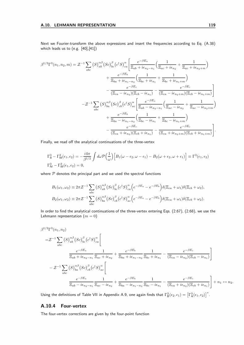
A.10. LEHMANN REPRESENTATION 119
Next we Fourier-transform the above expressions and insert the frequencies according to Eq. (A.38)which leads us to (e.g. [40],[41])
β1/2Γ3(n1, n2,m) = Z−1∑
abc
(S)αβ
ab
(Sc)β
bc
(c†S)α
ca
[
e−βEa
Ξab + iǫn2−n1
( 1
Ξac + iǫn2
+1
Ξac + iǫn2+m
)
+e−βEb
Ξba + iǫn1−n2
( 1
Ξbc + iǫn1
+1
Ξbc + iǫn1+m
)
− e−βEc
(Ξca − iǫn2)(Ξcb − iǫn1)− e−βEc
(Ξca − iǫn2+m)(Ξcb − iǫn1+m)
]
−Z−1∑
abc
(S)αβ
ba
(Sc)β
cb
(c†S)α
ac
[
e−βEa
Ξab − iǫn2−n1
( 1
Ξac − iǫn2
+1
Ξac − iǫn2+m
)
+e−βEb
Ξba − iǫn1−n2
( 1
Ξbc − iǫn1
+1
Ξbc − iǫn1+m
)
− e−βEc
(Ξca + iǫn2)(Ξcb + iǫn1)− e−βEc
(Ξca + iǫn2+m)(Ξcb + iǫn1+m)
]
.
Finally, we read off the analytical continuations of the three-vertex
Γ3II − Γ3
III(ǫ1, ǫ2) = − i4π
β1/2
∫
dωP( 1
ω
)[
B1(ω − ǫ2, ω − ǫ1) −B2(ω + ǫ2, ω + ǫ1)]
≡ Γ3(ǫ1, ǫ2)
Γ3IV − Γ3
III(ǫ1, ǫ2) = 0,
where P denotes the principal part and we used the spectral functions
B1(ω1, ω2) ≡ 2πZ−1∑
abc
(S)αβ
ab
(Sc)β
bc
(c†S)α
ca
(
e−βEa − e−βEb
)
δ(Ξca + ω1)δ(Ξcb + ω2),
B2(ω1, ω2) ≡ 2πZ−1∑
abc
(S)αβ
ba
(Sc)β
cb
(c†S)α
ac
(
e−βEa − e−βEb
)
δ(Ξca + ω1)δ(Ξcb + ω2).
In order to find the analytical continuations of the three-vertex entering Eqs. (2.67), (2.68), we use theLehmann representation (m = 0)
β1/2Γ3(n1, n2)
=Z−1∑
abc
(S)αβ
ab
(Sc)β
bc
(c†S)α
ca
[
e−βEa
Ξab + iǫn2−n1
1
Ξac + iǫn2
+e−βEb
Ξba + iǫn1−n2
1
Ξbc + iǫn1
− e−βEc
(Ξca − iǫn2)(Ξcb − iǫn1)
]
−Z−1∑
abc
(S)αβ
ba
(Sc)β
cb
(c†S)α
ac
[
e−βEa
Ξab − iǫn2−n1
1
Ξac − iǫn2
+e−βEb
Ξba − iǫn1−n2
1
Ξbc − iǫn1
− e−βEc
(Ξca + iǫn2)(Ξcb + iǫn1)
]
+ n1 ↔ n2.
Using the definitions of Table VII in Appendix A.9, one again finds that Γ3B(ǫ2, ǫ1) =
[Γ3
A(ǫ1, ǫ2)]∗
.
A.10.4 Four-vertex
The four-vertex corrections are given by the four-point function

120 APPENDIX A. APPENDIX (DEPHASING BY KONDO IMPURITIES)
Γ4(n1, n2,m) ≡⟨(Sc)α
n1+m
(c†S)β
n2+m
(Sc)β
n2
(c†S)α
n1
⟩,
or in (imaginary-) time representation
Γ4(n1, n2,m) ≡ 1
β2
∫
dτ1dτ2dτ3dτ4eiǫn1+mτ1+iǫn2τ2−iǫn2+mτ3−iǫn1τ4
⟨Tτ (Sc)
α(τ1)(Sc)β(τ2)(Sc
†)β(τ3)(Sc†)α(τ4)
⟩.
Again, we start from the time-ordered product
Γ4(τ1τ2τ3τ4) ≡⟨Tτ (Sc)
α(τ1)(Sc)β(τ2)(Sc
†)β(τ3)(Sc†)α(τ4)
⟩
Following the same strategy as before we group the 24 terms of the time-ordered product in six familiesarising from cyclic permutations, i.e.
Γ4 = Γ41234 − Γ4
1243 − Γ41324 + Γ4
1342 + Γ41423 − Γ4
1432.
The family emerging from the order 1 > 2 > 3 > 4 has the Lehmann representation
Γ41234(τ1τ2τ3τ4)
= Z−1∑
abcd
(Sc)α
ab
(Sc)β
bc
(Sc†)β
cd
(Sc†)α
da
[
e−βEaeΞab(τ1−τ2)+Ξac(τ2−τ3)+Ξad(τ3−τ4)Θ1234 − e−βEbeΞbc(τ2−τ3)+Ξbd(τ3−τ4)+Ξba(τ4−τ1)Θ2341
+ e−βEceΞcd(τ3−τ4)+Ξca(τ4−τ1)+Ξcb(τ1−τ2)Θ3412 − e−βEdeΞda(τ4−τ1)+Ξdb(τ1−τ2)+Ξdc(τ2−τ3)Θ4123
]
The contributions corresponding to cycles from the remaining orders are
Γ41243(τ1τ2τ3τ4)
= Z−1∑
abcd
(Sc)α
ab
(Sc)β
bc
(Sc†)α
cd
(Sc†)β
da
[
e−βEaeΞab(τ1−τ2)+Ξac(τ2−τ4)+Ξad(τ4−τ3)Θ1243 − e−βEbeΞbc(τ2−τ4)+Ξbd(τ4−τ3)+Ξba(τ3−τ1)Θ2431
+ e−βEceΞcd(τ4−τ3)+Ξca(τ3−τ1)+Ξcb(τ1−τ2)Θ4312 − e−βEdeΞda(τ3−τ1)+Ξdb(τ1−τ2)+Ξdc(τ2−τ4)Θ3124
]
Γ41324(τ1τ2τ3τ4)
= Z−1∑
abcd
(Sc)α
ab
(Sc†)β
bc
(Sc)β
cd
(Sc†)α
da
[
e−βEaeΞab(τ1−τ3)+Ξac(τ3−τ2)+Ξad(τ2−τ4)Θ1324 − e−βEbeΞbc(τ3−τ2)+Ξbd(τ2−τ4)+Ξba(τ4−τ1)Θ3241
+ e−βEceΞcd(τ2−τ4)+Ξca(τ4−τ1)+Ξcb(τ1−τ3)Θ2413 − e−βEdeΞda(τ4−τ1)+Ξdb(τ1−τ3)+Ξdc(τ3−τ2)Θ4132
]
Γ41342(τ1τ2τ3τ4)
= Z−1∑
abcd
(Sc)α
ab
(Sc†)β
bc
(Sc†)α
cd
(Sc)β
da
[
e−βEaeΞab(τ1−τ3)+Ξac(τ3−τ4)+Ξad(τ4−τ2)Θ1342 − e−βEbeΞbc(τ3−τ4)+Ξbd(τ4−τ2)+Ξba(τ2−τ1)Θ3421
+ e−βEceΞcd(τ4−τ2)+Ξca(τ2−τ1)+Ξcb(τ1−τ3)Θ4213 − e−βEdeΞda(τ2−τ1)+Ξdb(τ1−τ3)+Ξdc(τ3−τ4)Θ2134
]

A.10. LEHMANN REPRESENTATION 121
Γ41423(τ1τ2τ3τ4)
= Z−1∑
abcd
(Sc)α
ab
(Sc†)α
bc
(Sc)β
cd
(Sc†)β
da
[
e−βEaeΞab(τ1−τ4)+Ξac(τ4−τ2)+Ξad(τ2−τ3)Θ1423 − e−βEbeΞbc(τ4−τ2)+Ξbd(τ2−τ3)+Ξba(τ3−τ1)Θ4231
+ e−βEceΞcd(τ2−τ3)+Ξca(τ3−τ1)+Ξcb(τ1−τ4)Θ2314 − e−βEdeΞda(τ3−τ1)+Ξdb(τ1−τ4)+Ξdc(τ4−τ2)Θ3142
]
Γ41432(τ1τ2τ3τ4)
= Z−1∑
abcd
(Sc)α
ab
(Sc†)α
bc
(Sc†)β
cd
(Sc)β
da
[
e−βEaeΞab(τ1−τ4)+Ξac(τ4−τ3)+Ξad(τ3−τ2)Θ1432 − e−βEbeΞbc(τ4−τ3)+Ξbd(τ3−τ2)+Ξba(τ2−τ1)Θ4321
+ e−βEceΞcd(τ3−τ2)+Ξca(τ2−τ1)+Ξcb(τ1−τ4)Θ3214 − e−βEdeΞda(τ2−τ1)+Ξdb(τ1−τ4)+Ξdc(τ4−τ3)Θ2143
]
.
Analogue to the three-vertex we bring it into a “nicer” form by exchanging a ↔ b and c ↔ d in thefourth, fifth and sixth term and grouping the first with the sixth, the second with the fourth and thethird with the fifth term
Γ41234 − Γ4
1432
= Z−1∑
abcd
(Sc)α
ab
(Sc)β
bc
(Sc†)β
cd
(Sc†)α
da
[
e−βEaeΞab(τ1−τ2)+Ξac(τ2−τ3)+Ξad(τ3−τ4)Θ1234 − e−βEbeΞbc(τ2−τ3)+Ξbd(τ3−τ4)+Ξba(τ4−τ1)Θ2341
+ e−βEceΞcd(τ3−τ4)+Ξca(τ4−τ1)+Ξcb(τ1−τ2)Θ3412 − e−βEdeΞda(τ4−τ1)+Ξdb(τ1−τ2)+Ξdc(τ2−τ3)Θ4123
]
−(Sc)αba(Sc†)α
ad
(Sc†)β
dc
(Sc)β
cb
[
e−βEaeΞba(τ1−τ2)+Ξca(τ2−τ3)+Ξda(τ3−τ4)Θ4321 − e−βEbeΞcb(τ2−τ3)+Ξdb(τ3−τ4)+Ξab(τ4−τ1)Θ1432
+ e−βEceΞdc(τ3−τ4)+Ξac(τ4−τ1)+Ξbc(τ1−τ2)Θ2143 − e−βEdeΞad(τ4−τ1)+Ξbd(τ1−τ2)+Ξcd(τ2−τ3)Θ3214
]
Γ41243 − Γ4
1342
= Z−1∑
abcd
(Sc)α
ab
(Sc)β
bc
(Sc†)α
cd
(Sc†)β
da
[
e−βEaeΞab(τ1−τ2)+Ξac(τ2−τ4)+Ξad(τ4−τ3)Θ1243 − e−βEbeΞbc(τ2−τ4)+Ξbd(τ4−τ3)+Ξba(τ3−τ1)Θ2431
+ e−βEceΞcd(τ4−τ3)+Ξca(τ3−τ1)+Ξcb(τ1−τ2)Θ4312 − e−βEdeΞda(τ3−τ1)+Ξdb(τ1−τ2)+Ξdc(τ2−τ4)Θ3124
]
−(Sc)α
ba
(Sc†)β
ad
(Sc†)α
dc
(Sc)β
cb
[
e−βEaeΞba(τ1−τ2)+Ξca(τ2−τ4)+Ξda(τ4−τ3)Θ3421 − e−βEbeΞcb(τ2−τ4)+Ξdb(τ4−τ3)+Ξab(τ3−τ1)Θ1342
+ e−βEceΞdc(τ4−τ3)+Ξac(τ3−τ1)+Ξbc(τ1−τ2)Θ2134 − e−βEdeΞad(τ3−τ1)+Ξbd(τ1−τ2)+Ξcd(τ2−τ4)Θ4213
]

122 APPENDIX A. APPENDIX (DEPHASING BY KONDO IMPURITIES)
Γ41324 − Γ4
1423
= Z−1∑
abcd
(Sc)α
ab
(Sc†)β
bc
(Sc)β
cd
(Sc†)α
da
[
e−βEaeΞab(τ1−τ3)+Ξac(τ3−τ2)+Ξad(τ2−τ4)Θ1324 − e−βEbeΞbc(τ3−τ2)+Ξbd(τ2−τ4)+Ξba(τ4−τ1)Θ3241
+ e−βEceΞcd(τ2−τ4)+Ξca(τ4−τ1)+Ξcb(τ1−τ3)Θ2413 − e−βEdeΞda(τ4−τ1)+Ξdb(τ1−τ3)+Ξdc(τ3−τ2)Θ4132
]
−(Sc)α
ba
(Sc†)α
ad
(Sc)β
dc
(Sc†)β
cb
[
e−βEaeΞba(τ1−τ3)+Ξca(τ3−τ2)+Ξda(τ2−τ4)Θ4231 − e−βEbeΞcb(τ3−τ2)+Ξdb(τ2−τ4)+Ξab(τ4−τ1)Θ1423
+ e−βEceΞdc(τ2−τ4)+Ξac(τ4−τ1)+Ξbc(τ1−τ3)Θ3142 − e−βEdeΞad(τ4−τ1)+Ξbd(τ1−τ3)+Ξcd(τ3−τ2)Θ2314
]
.
Fourier-transformation then leads to (see also [40])
Γ41234 − Γ4
1432
= β−1Z−1∑
abcd
(Sc)α
ab
(Sc)β
bc
(Sc†)β
cd
(Sc†)α
da
[
e−βEa
(Ξab + iǫn1+m)(Ξac + iǫn1+n2+m)(Ξad + iǫn1)− e−βEb
(Ξbc + iǫn2)(Ξbd − iωm)(Ξba − iǫn1+m)
+e−βEc
(Ξcd − iǫn2+m)(Ξca − iǫn1+n2+m)(Ξcb − iǫn2)− e−βEd
(Ξda − iǫn1)(Ξdb + iωm)(Ξdc + iǫn2+m)
]
+(Sc)α
ba
(Sc†)α
ad
(Sc†)β
dc
(Sc)β
cb
[
e−βEa
(Ξab − iǫn1+m)(Ξac − iǫn1+n2+m)(Ξad − iǫn1)− e−βEb
(Ξbc − iǫn2)(Ξbd + iωm)(Ξba + iǫn1+m)
+e−βEc
(Ξcd + iǫn2+m)(Ξca + iǫn1+n2+m)(Ξcb + iǫn2)− e−βEd
(Ξda + iǫn1)(Ξdb − iωm)(Ξdc − iǫn2+m)
]
Γ41243 − Γ4
1342
= β−1Z−1∑
abcd
(Sc)α
ab
(Sc)β
bc
(Sc†)α
cd
(Sc†)β
da
[
e−βEa
(Ξab + iǫn1+m)(Ξac + iǫn1+n2+m)(Ξad + iǫn2+m)− e−βEb
(Ξbc + iǫn2)(Ξbd − iǫn1−n2)(Ξba − iǫn1+m)
+e−βEc
(Ξcd − iǫn1)(Ξca − iǫn1+n2+m)(Ξcb − iǫn2)− e−βEd
(Ξda − iǫn2+m)(Ξdb + iǫn1−n2)(Ξdc + iǫn1)
]
+(Sc)α
ba
(Sc†)β
ad
(Sc†)α
dc
(Sc)β
cb
[
e−βEa
(Ξab − iǫn1+m)(Ξac − iǫn1+n2+m)(Ξad − iǫn2+m)− e−βEb
(Ξbc − iǫn2)(Ξbd + iǫn1−n2)(Ξba + iǫn1+m)
+e−βEc
(Ξcd + iǫn1)(Ξca + iǫn1+n2+m)(Ξcb + iǫn2)− e−βEd
(Ξda + iǫn2+m)(Ξdb − iǫn1−n2)(Ξdc − iǫn1)
]

A.10. LEHMANN REPRESENTATION 123
Γ41324 − Γ4
1423
= β−1Z−1∑
abcd
(Sc)α
ab
(Sc†)β
bc
(Sc)β
cd
(Sc†)α
da
[
e−βEa
(Ξab + iǫn1+m)(Ξac + iǫn1−n2)(Ξad + iǫn1)− e−βEb
(Ξbc − iǫn2+m)(Ξbd − iωm)(Ξba − iǫn1+m)
+e−βEc
(Ξcd + iǫn2)(Ξca − iǫn1−n2)(Ξcb + iǫn2+m)− e−βEd
(Ξda − iǫn1)(Ξdb + iωm)(Ξdc − iǫn2)
]
+(Sc)α
ba
(Sc†)α
ad
(Sc)β
dc
(Sc†)β
cb
[
e−βEa
(Ξab − iǫn1+m)(Ξac − iǫn1−n2)(Ξad − iǫn1)− e−βEb
(Ξbc + iǫn2+m)(Ξbd + iωm)(Ξba + iǫn1+m)
+e−βEc
(Ξcd − iǫn2)(Ξca + iǫn1−n2)(Ξcb − iǫn2+m)− e−βEd
(Ξda + iǫn1)(Ξdb − iωm)(Ξdc + iǫn2)
]
.
The analytical continuation leads to the following functions
Γ41(ǫ1, ǫ2) ≡ Γ4
II − Γ4III(ǫ1, ǫ2) =iβ−1
∫
dω1dω21
ω1 + ǫ1 + i0
(C1(ω1, ǫ2 − ǫ1, ω2)
ω2 + ǫ1 − i0− D1(ω1, ǫ2 − ǫ1, ω2)
ω2 − ǫ2 + i0
)
− iβ−1
∫
dω1dω21
ω1 − ǫ1 − i0
(C2(ω1,−ǫ2 + ǫ1, ω2)
ω2 − ǫ1 + i0− D2(ω1,−ǫ2 + ǫ1, ω2)
ω2 + ǫ2 − i0
)
,
where we introduced the following spectral densities
C1(ω1, ω2, ω3) ≡ 2πZ−1∑
abcd
(Sc)α
ab
(Sc)β
cd
(Sc†)β
bc
(Sc†)α
da
(
e−βEa − e−βEc
)
δ(Ξba + ω1)δ(Ξca + ω2)δ(Ξda + ω3)
C2(ω1, ω2, ω3) ≡ 2πZ−1∑
abcd
(Sc)α
ba
(Sc)β
dc
(Sc†)β
cb
(Sc†)α
ad
(
e−βEa − e−βEc
)
δ(Ξba + ω1)δ(Ξca + ω2)δ(Ξda + ω3)
D1(ω1, ω2, ω3) ≡ 2πZ−1∑
abcd
(Sc)α
ab
(Sc)β
da
(Sc†)β
bc
(Sc†)α
cd
(
e−βEa − e−βEc
)
δ(Ξba + ω1)δ(Ξca + ω2)δ(Ξda + ω3)
D2(ω1, ω2, ω3) ≡ 2πZ−1∑
abcd
(Sc)α
ba
(Sc)β
ad
(Sc†)β
cb
(Sc†)α
dc
(
e−βEa − e−βEc
)
δ(Ξba + ω1)δ(Ξca + ω2)δ(Ξda + ω3)
and
Γ42(ǫ1, ǫ2) ≡ Γ4
III − Γ4IV(ǫ1, ǫ2) = − iβ−1
∫
dω1dω21
ω1 + ǫ1 + i0
(C3(ω1,−ǫ2 − ǫ1, ω2)
ω2 + ǫ1 − i0− D3(ω1,−ǫ2 − ǫ1, ω2)
ω2 + ǫ2 + i0
)
+ iβ−1
∫
dω1dω21
ω1 − ǫ1 − i0
(C4(ω1, ǫ2 + ǫ1, ω2)
ω2 − ǫ1 + i0− D4(ω1, ǫ2 + ǫ1, ω2)
ω2 − ǫ2 − i0
)
,
where
C3(ω1, ω2, ω3) ≡ 2πZ−1∑
abcd
(Sc)α
ab
(Sc)β
bc
(Sc†)β
cd
(Sc†)α
da
(
e−βEa − e−βEc
)
δ(Ξba + ω1)δ(Ξca + ω2)δ(Ξda + ω3)
C4(ω1, ω2, ω3) ≡ 2πZ−1∑
abcd
(Sc)α
ba
(Sc)β
cb
(Sc†)β
dc
(Sc†)α
ad
(
e−βEa − e−βEc
)
δ(Ξba + ω1)δ(Ξca + ω2)δ(Ξda + ω3)
D3(ω1, ω2, ω3) ≡ 2πZ−1∑
abcd
(Sc)α
ab
(Sc)β
bc
(Sc†)β
da
(Sc†)α
cd
(
e−βEa − e−βEc
)
δ(Ξba + ω1)δ(Ξca + ω2)δ(Ξda + ω3)
D4(ω1, ω2, ω3) ≡ 2πZ−1∑
abcd
(Sc)α
ba
(Sc)β
cb
(Sc†)β
ad
(Sc†)α
dc
(
e−βEa − e−βEc
)
δ(Ξba + ω1)δ(Ξca + ω2)δ(Ξda + ω3)
Again, it can be seen that Γ4B(ǫ2, ǫ1) =
[Γ4
B(ǫ1, ǫ1)]∗
.Summarizing, we find the following analytical continuations of Γin

124 APPENDIX A. APPENDIX (DEPHASING BY KONDO IMPURITIES)
Γ2(ǫ1, ǫ2) = iA(ǫ2 − ǫ1)
Γ3(ǫ1, ǫ2) = − i2
β1/2
∫
dωP( 1
ω
)[
B1(ω − ǫ2, ω − ǫ1) −B2(ω + ǫ2, ω + ǫ1)]
Γ41(ǫ1, ǫ2) = iβ−1
∫
dω1dω21
ω1 + ǫ1 + i0
(C1(ω1, ǫ2 − ǫ1, ω2)
ω2 + ǫ1 − i0− D1(ω1, ǫ2 − ǫ1, ω2)
ω2 − ǫ2 + i0
)
− iβ−1
∫
dω1dω21
ω1 − ǫ1 − i0
(C2(ω1,−ǫ2 + ǫ1, ω2)
ω2 − ǫ1 + i0− D2(ω1,−ǫ2 + ǫ1, ω2)
ω2 + ǫ2 − i0
)
Γ42(ǫ1, ǫ2) = −iβ−1
∫
dω1dω21
ω1 + ǫ1 + i0
(C3(ω1,−ǫ2 − ǫ1, ω2)
ω2 + ǫ1 − i0− D3(ω1,−ǫ2 − ǫ1, ω2)
ω2 + ǫ2 + i0
)
+ iβ−1
∫
dω1dω21
ω1 − ǫ1 − i0
(C4(ω1, ǫ2 + ǫ1, ω2)
ω2 − ǫ1 + i0− D4(ω1, ǫ2 + ǫ1, ω2)
ω2 − ǫ2 − i0
)
Looking at the integrals over ǫ1, ǫ2 (see Eqs. (2.67), (2.68)) we notice that we can exchange ǫi → −ǫiin the second terms of Γ3 and Γ4, i.e.
Γ2(ǫ1, ǫ2) = iA(ǫ2 − ǫ1)
Γ3(ǫ1, ǫ2) =i2
β1/2
∫
dωP( 1
ω
)[
B1(ω + ǫ2, ω + ǫ1) +B2(ω + ǫ2, ω + ǫ1)]
Γ41(ǫ1, ǫ2) = iβ−1
∫
dω1dω2
[
C1(ω1, ǫ2 − ǫ1, ω2)
(ω1 + ǫ1 + i0)(ω2 + ǫ1 − i0)+
C2(ω1, ǫ2 − ǫ1, ω2)
(ω1 + ǫ1 − i0)(ω2 + ǫ1 + i0)
− D1(ω1, ǫ2 − ǫ1, ω2)
(ω1 + ǫ1 + i0)(ω2 − ǫ2 + i0)− D2(ω1, ǫ2 − ǫ1, ω2)
(ω1 + ǫ1 − i0)(ω2 − ǫ2 − i0)
]
Γ42(ǫ1, ǫ2) = −iβ−1
∫
dω1dω2
[
C3(ω1,−ǫ1 − ǫ2, ω2)
(ω1 + ǫ1 + i0)(ω2 + ǫ1 − i0)+
C4(ω1,−ǫ1 − ǫ2, ω2)
(ω1 + ǫ1 − i0)(ω2 + ǫ1 + i0)
− D3(ω1,−ǫ1 − ǫ2, ω2)
(ω1 + ǫ1 + i0)(ω2 + ǫ2 + i0)− D4(ω1,−ǫ1 − ǫ2, ω2)
(ω1 + ǫ1 − i0)(ω2 + ǫ2 − i0
]
.
The spectral functions are given by

A.10. LEHMANN REPRESENTATION 125
ImΣR(ω) ≡ −πZ−1∑
ab
(Sc)αab(c†S)αba
(
e−βEa + e−βEb
)
δ(Ξab + ω)
A(ω) ≡ 2πZ−1∑
ab
SαabSαba
(
e−βEa − e−βEb
)
δ(Ξab + ω)
B1(ω1, ω2) ≡ 2πZ−1∑
abc
(S)αβ
ab
(Sc)β
bc
(c†S)α
ca
(
e−βEa − e−βEb
)
δ(Ξac + ω1)δ(Ξbc + ω2)
B2(ω1, ω2) ≡ 2πZ−1∑
abc
(S)αβ
ba
(Sc)β
cb
(c†S)α
ac
(
e−βEa − e−βEb
)
δ(Ξac + ω1)δ(Ξbc + ω2)
C1(ω1, ω2, ω3) ≡ 2πZ−1∑
abcd
(Sc)α
ab
(Sc)β
cd
(Sc†)β
bc
(Sc†)α
da
(
e−βEa − e−βEc
)
δ(Ξba + ω1)δ(Ξca + ω2)δ(Ξda + ω3)
C2(ω1, ω2, ω3) ≡ 2πZ−1∑
abcd
(Sc)α
ba
(Sc)β
dc
(Sc†)β
cb
(Sc†)α
ad
(
e−βEa − e−βEc
)
δ(Ξba + ω1)δ(Ξca + ω2)δ(Ξda + ω3)
D1(ω1, ω2, ω3) ≡ 2πZ−1∑
abcd
(Sc)α
ab
(Sc)β
da
(Sc†)β
bc
(Sc†)α
cd
(
e−βEa − e−βEc
)
δ(Ξba + ω1)δ(Ξca + ω2)δ(Ξda + ω3)
D2(ω1, ω2, ω3) ≡ 2πZ−1∑
abcd
(Sc)α
ba
(Sc)β
ad
(Sc†)β
cb
(Sc†)α
dc
(
e−βEa − e−βEc
)
δ(Ξba + ω1)δ(Ξca + ω2)δ(Ξda + ω3)
C3(ω1, ω2, ω3) ≡ 2πZ−1∑
abcd
(Sc)α
ab
(Sc)β
bc
(Sc†)β
cd
(Sc†)α
da
(
e−βEa − e−βEc
)
δ(Ξba + ω1)δ(Ξca + ω2)δ(Ξda + ω3)
C4(ω1, ω2, ω3) ≡ 2πZ−1∑
abcd
(Sc)α
ba
(Sc)β
cb
(Sc†)β
dc
(Sc†)α
ad
(
e−βEa − e−βEc
)
δ(Ξba + ω1)δ(Ξca + ω2)δ(Ξda + ω3)
D3(ω1, ω2, ω3) ≡ 2πZ−1∑
abcd
(Sc)α
ab
(Sc)β
bc
(Sc†)β
da
(Sc†)α
cd
(
e−βEa − e−βEc
)
δ(Ξba + ω1)δ(Ξca + ω2)δ(Ξda + ω3)
D4(ω1, ω2, ω3) ≡ 2πZ−1∑
abcd
(Sc)α
ba
(Sc)β
cb
(Sc†)β
ad
(Sc†)α
dc
(
e−βEa − e−βEc
)
δ(Ξba + ω1)δ(Ξca + ω2)δ(Ξda + ω3).

126 APPENDIX A. APPENDIX (DEPHASING BY KONDO IMPURITIES)

Appendix B
Appendix (Disordered LuttingerLiquid)
B.1 l0-independent contributions from the “ tr ln ”-expansion
In this appendix we want to show that there are no further l0-independent contributions from the“ tr ln”-expansion than those considered in the text, i.e. the term depending on T from the linear orderexpansion, S(1)[T ], and the term where T equals to the unit matrix from the second order expansion,S(2)[T ]. To this end we go back to the series-expansion of the “ tr ln ”,
S[T,X1, X2] =1
2
∑
k=1
(−1)k
ktrGΛ [X1 +X2]
k,
where
X1ττ ′(x) =
[T−1(∂T )
]
ττ ′ (x) (B.1)
X2ττ ′(x) =
[T−1
[µ+ iaσ3σ
T3
]T]
ττ ′ (x). (B.2)
For a systematic analysis of the various contributions we introduce the matrix Oττ ′(x) which is localin space and non-local in time and the field φ(x, τ) both local in space and time. φ represents thesource-fields (or a fluctuating “interaction”-field) and results from X2 with T and T−1 being the unitmatrices, while O resembles the remaining contributions. To be precise, O takes into account X1 andthose contributions from X2 in which at least one of the matrices T or T−1 differs from 1. Notice thatin energy-representation Onn′ is only non-vanishing inside an energy range |n|, |n′| < n0 where ǫn0 issome high-energy-scale limiting the applicability of our low-energy model. So let us take a look at theterms from the expansion depending only on φ,
S[φ] =1
2
∑
k=1
(−1)k
ktrGΛφ
k.
In energy/momentum representation the k-th order takes the form (for convenience we here restrict tothe +-sector)
127

128 APPENDIX B. APPENDIX (DISORDERED LUTTINGER LIQUID)
trg+Λφk
=∑
n
∑
m1
...∑
mk−1
∫
dp
∫
dq1...
∫
dqk1
1
z ± i2l0
1
z + z1 ± i2l0
1
z + z1 + z2 ± i2l0
...1
z + z1 + z2 + ...+ zk−1 ± i2l0
φ(z1)φ(z2)φ(z3)...φ(zk)φ(−z1 − z2 − ...− zk)
=∑
n
∑
m1
...∑
mk−1
∫
dp
∫
dq1...
∫
dqk1Γk(z, z1, ...zk−1)φ(z1)φ...φ(zk)φ(−z1 − z2 − ...− zk),
where we introduced the short notation z = p + iǫn and zi = qi + iωmi and the sign ± i2l0
is thatof ǫn. We may now divide the energy-sums into a part, where all energies have the same sign (i.e.all Greens functions g+ are either all retarded or all advanced) and a part where the product of thek Greens functions contains g+ with different causal structure. Starting with the later we use that
1z+z1± i
2l0
= 1z± i
2l0
∑∞l=0
zl1
[z± i2l0
]lin order to write
Γk(z, z1, ...zk−1)
=
∞∑
l1=0
...
∞∑
lk−1=0
1
[z ± i2l0
]k1
[z ± i2l0
]l11
[z ± i2l0
]l2...
1
[z ± i2l0
]lk−1zl11 (z1 + z2)
l2 ...(z1 + ...zk−1)lk−1 .
Performing the ǫ-integral we find
∫
dǫΓk(z, z1, ...zk−1) ∝∞∑
l1=0
...
∞∑
lk−1=0
lk−10 (l0z1)
l1(l0[z1 + z2])l2 ...(l0[z1 + ...zk−1])
lk−1 ,
which vanishes for l0 = 0 (as discussed in the text keeping only the l0-independent contributions wemay equally set l0 in the calculations). Notice that taking l0 = 0 is well-defined as all remainingintegrals are convergent:
∫dp due to momentum cut-off Λ and those over ωmi and qi due to φ(ωi, qi).
This procedure works for k > 1. For k = 1 the source-field has vanishing arguments, φ(z1 = 0), andtherefore is zero.
Next we turn to the case where all g+ are either retarded or advanced, e.g.
Γk(z, z1, ...zk−1)
=∞∑
l1=0
...∞∑
lk−1=0
1
[z − i2l0
]k1
[z − i2l0
]l11
[z − i2l0
]l2...
1
[z − i2l0
]lk−1zl11 (z1 + z2)
l2 ...(z1 + ...zk−1)lk−1
=
∞∑
l1=0
...
∞∑
lk−1=0
1
[z − i2l0
]k+l1+...+lk−1zl11 (z1 + z2)
l2 ...(z1 + ...zk−1)lk−1 .
In this case we first integrate over ǫ (which for advance g+ has to be positive) and then over p, i.e.
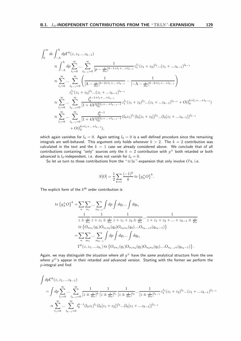
B.1. L0-INDEPENDENT CONTRIBUTIONS FROM THE “ TRLN”-EXPANSION 129
∫ ∞
0
dǫ
∫ Λ
−Λ
dpΓk(z, z1, ...zk−1)
∝∫ Λ
−Λ
dp
∞∑
l1=0
...
∞∑
lk−1=0
1
[p− i2l0
]k−1+l1+...+lk−1zl11 (z1 + z2)
l2 ...(z1 + ...zk−1)lk−1
∝∞∑
l1=0
...∞∑
lk−1=0
(
1
[Λ − i2l0
]k−2+l1+...+lk−1− 1
[−Λ − i2l0
]k−2+l1+...+lk−1
)
zl11 (z1 + z2)l2 ...(z1 + ...zk−1)
lk−1
∝∞∑
l1=0
...
∞∑
lk−1=0
lk−1+l1+...+lk−1
0
[1 + 4Λ2l20]l1+...+lk−1−1
zl11 (z1 + z2)l2 ...(z1 + ...zk−1)
lk−1 +O(lk+l1+...+lk−1
0 )
∝∞∑
l1=0
...
∞∑
lk−1=0
lk−10
[1 + 4Λ2l20]l1+...+lk−1−1
(l0z1)l1(l0[z1 + z2])
l2 ...(l0[z1 + ...zk−1])lk−1
+O(lk+l1+...+lk−1
0 ),
which again vanishes for l0 = 0. Again setting l0 = 0 is a well defined procedure since the remainingintegrals are well-behaved. This argument only holds whenever k > 2. The k = 2 contribution wascalculated in the text and the k = 1 case we already considered above. We conclude that of allcontributions containing “only” sources only the k = 2 contribution with g± both retarded or bothadvanced is l0-independent, i.e. does not vanish for l0 = 0.
So let us turn to those contributions from the “ tr ln ”-expansion that only involve O’s, i.e.
S[O] =1
2
∑
k=1
(−1)k
ktrg+ΛOk.
The explicit form of the kth order contribution is
trg+ΛOk
=∑
n
∑
n1
...∑
nk−1
∫
dp
∫
dq1...
∫
dqk1
1
z ± i2l0
1
z + z1 ± i2l0
1
z + z1 + z2 ± i2l0
...1
z + z1 + z2 + ...+ zk−1 ± i2l0
trOnn1(q1)On1n2(q2)On2n3(q3)....Onk−1n(qnk−1)
=∑
n
∑
m1
...∑
mk−1
∫
dp
∫
dq1...
∫
dqk1
Γk(z, z1, ...zk1) trOnn1(q1)On1n2(q2)On2n3(q3)....Onk−1n(qnk−1)
.
Again, we may distinguish the situation where all g± have the same analytical structure from the onewhere g±’s appear in their retarded and advanced version. Starting with the former we perform thep-integral and find
∫
dpΓk(z, z1, ...zk−1)
=
∫
dp∞∑
l1=0
...∞∑
lk−1=0
1
[z ± i2l0
]k1
[z ± i2l0
]l11
[z ± i2l0
]l2...
1
[z ± i2l0
]lk−1zl11 (z1 + z2)
l2 ...(z1 + ...zk−1)lk−1
∝∞∑
l1=0
...
∞∑
lk−1=0
lk−10 (l0z1)
l1(l0[z1 + z2])l2 ...(l0[z1 + ...zk−1])
lk−1

130 APPENDIX B. APPENDIX (DISORDERED LUTTINGER LIQUID)
which again vanishes for l0 = 0 (the remaining integrals are well-behaved). Notice that this time it is thefact that Onn′ is only non-vanishing inside some energy range |n|, |n′| < n0 that makes the ǫ-integralsconvergent. In the case of plain sources we had to perform the ǫ-integral (i.e. the n-summation) asthis was not restricted. (In the above situation we cannot perform the ǫ-integral as O still depends onǫ). Again, this argument holds for k > 1 and the case k = 1 was considered in the text.
Turning to the situation of k > 1 where all g±’s have the same analytical structure we may performthe p-integral, by closing the contour in the half plane of the complex plane, where Γ(p) has no poles,e.g.
∫
dpΓk(z, z1, ...zk−1)
=
∫
dp1
z − i2l0
1
z + z1 − i2l0
1
z + z1 + z2 − i2l0
...1
z + z1 + z2 + ...+ zk−1 − i2l0
= 0.
Again, the remaining integrals are well behaved. We conclude, that the only non-vanishing contributionsfrom the expansion of “ tr ln” containing only O’s stems from the linear order expansion (i.e. k = 1).This term has been considered in the text.
Turning to terms from the “ tr ln”-expansion containing contributions from φ and O (case 3) weobserve that for k > 2 we may apply the same argument as in the case where all contributions containedonly φ’s (case 1). The reason therefore is that in case 3 there is always a free ǫ-integral, in the sensethat ǫ just enters in the g±. We may therefore perform the free ǫ-integral and the argument used in case1 applies. In the case of the k = 2 contribution, linear in φ and linear O we may apply the argumentused in the case of only O’s (case 2) as the energy-integrals are restricted due to the presence of O.Therefore all “mixed” contributions containing φ as well as O vanish.
To summarize: In this appendix we showed that the “ tr ln”-expansion has just two l0-independent(i.e. non-vanishing for l0 = 0) contributions. These are
• trGΛ
[µ+ iaσ3σ
T3
]GΛ
[µ+ iaσ3σ
T3
]
• trGΛT
−1[∂ + µ+ iaσ3σ
T3
]T,
where in the second expression at least one of the matrices T or T−1 has to differ from unity. Theseterms were considered in the text: The first term is the diamagnetic contribution second order in thesources, and the second term accounts for its paramagnetic contribution. The fact that going beyondthe second order in sources gives no further contributions results from the “higher-loop cancelation”, asstated in the text. In this sense our approach is closely related to the functional bosonization methodwith the difference lying in the fact, that in our approach the paramagnetic contributions are takeninto account by coupling to a bosonic matrix-field, introduced in order to decouple the disorder averageinduced interaction between the electrons.
B.2 Diagrammatic evaluation of the density/density correlation
function
In this appendix we supply the explicit calculation of the density/density correlation function for theGreen’s functions dressed by forward scattering disorder length, i.e.
g±n (p) =1
−iǫn ± p− i2l0
sgn(n). (B.3)
The paramagnetic contribution to the density/density correlation function is given by the sum of twodiagrams depicted in Fig.3.2, where the single particle lines consist of a retarded and an advancedcontribution. The individual contributions calculate as

B.3. REGULARIZATION OF THE PROPAGATOR 131
Re
T∑
−m<n<0
∫dp
2π
1
p+ q + iǫn+m + i2l0
1
p+ iǫn − i2l0
=1
2πIm
ωm
q + iωm + i/l0
(B.4)
= + D(ωm, q) =1
l0 − iq+iωm+il−1
0
=1
l0
1 − iql0 + ωml0ωml0 − iql0
(B.5)
Re
1
T
∑
−m<n<0
∫
dp
2π
1
p+ q + iǫn+m + i2l0
1
p+ iǫn − i2l0
2
×D(ωm, q)
=−ωm2πl0
Re
(1
q + iωm + i/l0
)21 − iql0 + ωml0ωml0 − iql0
=1
2πIm
ωm
(ωml0 − iql0)(q + iωm + i/l0)
. (B.6)
B.3 Regularization of the propagator
We stated in the text, that before considering higher loop corrections to the Gaussian propagator onehas to modify the model in order to account for the limit of resolution set by the momentum cut-offΛ. This is done in this appendix. To be precise, we “soften” the δ-correlated disorder by taking thecorrelation function
〈u(x)u(x′)〉u = 2l−10 δ(x− x′ + a),
where a is e.g. Gaussian distributed, p(a) = e−a2/λ2
. This choice corresponds to Gaussian distributeddisorder,
〈u(x)u(x′)〉 = 2l−10 e−(x−x′)2/λ2
.
In the following we take the correlation length λ ≪ l0 to be the smallest length-scale in the system(e.g. may think of λ as the lattice spacing, i.e. λ = Λ−1). Going through the same steps as before theHubbard-Stratonovich field is now Q = Q(x, x + a). As a is negligible small the saddle-point analysisis unchanged and the Goldstone-modes are Q(x, x + a) = T (x + a)ΛT−1(x). Since we can think ofa → 0 the only modification results in “regularizing ” the pole-integral of the first order term in theexpansion of “ tr ln”
∑
n
∫
dx trGΛn (x, x+ a)X1
nn(x+ a, x)
=1
L
∑
np
∑
mq
tr
GΛn,pT
−1±,nn+m(q) [ωm ± iq]T±,n+mn(−q)e−ia(p−q)
.
Using that
∑
p
g±n,pe−iap =
∫dp
2π
e−iap
±p− iǫn= ±θ(∓na)e−ǫna

132 APPENDIX B. APPENDIX (DISORDERED LUTTINGER LIQUID)
we find (notice the factor 1/2 compared to a = 0, since in the latter case: θ(sna)e−ǫna = 12 ) and we
neglect e−ǫa as it is irrelevant
S0reg.[T±] = −1
2
∑
nm,q
trΛnT
−1±,nn+m(q) [ωm ± iq] e±iaqθ(±na)T±,n+mn(−q)
.
In Gaussian approximation this leads to the Diffuson-action (notice that the factor two is compensatedby combining θ(sa) + θ(−sa) in order to get eisq|a|)
S0reg[Ds] = −
∑
m>0
∑
−m<n<0
∑
q
tr
Dffs,nn+m(q) [ωm + siq] eisq|a|Dff
s,n+mn(−q)
Averaging according to 〈...〉 =∫da(...)p(a) the regularized propagator now takes the form
〈Dffs,nn+m(x)Dff
s,n+mn(x′)〉S0reg
=
〈Dffs,nn+m(x)Dff
s,n+mn(x′)〉S0 , s(x− x′) > λ
0, s(x− x′) < λ.
That is, introducing Gaussian correlated disorder, with a finite, yet very small correlation length, λ,the effective particle-hole propagator gives only non-vanishing contributions if the particle (hole) travelat least over the distance λ. This is compatible with the fact that we consider left- and right movingparticles and use the UV cut-off Λ in all momentum integrals and therefore, e.g. the density-densitycorrelation function, 〈ρ±(x)ρ±(x′)〉, should only be evaluated for values |x − x′| > Λ−1 (we may setλ = Λ−1). In summary, softening the (unphysical) δ-correlated disorder sets the local (in the sensethat |x−x′| < Λ−1) particle-hole propagator to zero, but leaves it unchanged on regular scales & Λ−1.Notice also that the regularization only works this way because electrons and holes can only travel inone direction. All considerations made here also apply for the Cooperon. The source part of the action,Ssou remains unchanged.
B.4 Equivalence of Eq.(3.68) and Eq.(3.72)
In this appendix we want to show how to obtain Eq.(3.68) from Eq.(3.72). Starting out from
S[ϕ] + Ssou.[µ, a] =1
2
∫
d2xϕtG−1ϕ+ tr ln ∂ +1
2π
∫
d2x (J + ϕ)t Π(J + ϕ) , (B.7)
where
J =
(µ+ iaµ− ia
)
and Πm(q) =
(Π+m(q)
Π−m(q)
)
where Π±m(q) =
q
q ± iωm. (B.8)
We introduce some more matrices,
Dm(q) =
(q + iωm q + iωm−q + iωm q − iωm
)
(B.9)
Lm(q) = Dt−m(−q)Πm(q)Dm(q) =
(q2 iωmqiωmq q2
)
(B.10)
gm(q) = Dt−m(−q)G−1Dm(q) =
1
g1g2
(g2ω
2m + g1q
2 iωmq(g1 − g2)iωmq(g1 − g2) −g1ω2
m − g2q2
)
, (B.11)
and replace the “ tr ln ∂” by a bosonic field integral,
−∫
d2xχ∂χ→ 1
2
∫
d2xΘtLΘ, (B.12)

B.5. EQUIVALENCE OF EQ.(3.72) AND EQ.(3.74) 133
where Θ =
(θ1θ2
)
. Now we introduce ϕ = DK and shift Θ → Θ − π−1/2[D−1J +K
]leading to
S[K]+S[Θ] + Ssou.[µ, a]
=1
2
∫
d2xKtgK +1
2
∫
d2xΘtLΘ +1
2π
∫
d2x(D−1J +K
)tL(D−1J +K
)
→ 1
2
∫
d2xKtgK +1
2
∫
d2xΘtLΘ +1
2√π
∫
d2x[ (D−1J +K
)tLΘ + ΘL
(D−1J +K
)]
.
Integration over K and then over Θ gives
1
2
∫
d2xKtgK +1
2
∫
d2xΘtLΘ +1
2√π
∫
d2x[ (D−1J +K
)tLΘ + ΘL
(D−1J +K
)]
→ 1
2
∫
d2xΘt[L+ Ltg−1L
]Θ +
1
2√π
∫
d2x[J tΠDΘ + ΘtDtΠJ
]
→ 1
2π
∫
d2xJ tΠD[L+ Ltg−1L
]−1DtΠJ
Finally, applying that
ΠD = iq
(1 −11 1
)
L+ Ltg−1L =
((1 − g2
2π
)q2 iωmq
iωmq(1 + g2
2π
)q2
)
(B.13)
one returns to action Eq. (3.68), i.e.
S[a, µ]
=1
2π
∑
m,q
vq2
v2q2 + ω2m
[gµmqµ−m,−q − g−1amqa−m,−q
]+
ωmq
v2q2 + ω2m
[µmqa−m,−q + amqµ−m,−q]
.
(B.14)
B.5 Equivalence of Eq.(3.72) and Eq.(3.74)
In this appendix we want to show the equivalence of Eq.(3.72) and Eq.(3.74). To this end we merelyhave to make sure that
tr lnG−1
Λ
= tr ln
G−1
0
,
where G0 = ∂−1 and GΛ = [∂ − i2l0
Λ]−1. Since
tr lnG−1
Λ
= tr ln
∂
+ tr ln1 +
i
2l0G0Λ
,
this is amounts to showing that
tr ln1 +
i
2l0G0Λ
= 0,
and may be done as follows:

134 APPENDIX B. APPENDIX (DISORDERED LUTTINGER LIQUID)
tr ln
1 +i
2l0G0Λ
= −∞∑
k=1
1
ktr
i
2l0G0Λ
k
= −∞∑
k=1
1
k
∑
n,p
tr
i
2l0G0(n, p)Λn
k
= −∞∑
k=1
1
k
∑
|p|<Λ
(∑
n>0
[ i
2l0g+0 (n, p)
]k+[ i
2l0g−0 (n, p)
]k
+∑
n<0
[−i2l0
g+0 (n, p)
]k+[−i2l0
g−0 (n, p)]k)
Substituting g±n (p) = −1iǫn∓p we get
1
k
∑
n>0
[i
2l0g±n (p)
]k
=1
k
∑
n>0
( −i2l0[iǫn ∓ p]
)k
=T
k
∫ ∞
0
dǫ
2π
( −1
2l0[ǫ± ip]
)k
= − T
2π
( ±i2l0p
)k−1
1
k
∑
n<0
[−i2l0
g±n (p)
]k
=1
k
∑
n<0
(i
2l0[iǫn ∓ p]
)k
=T
k
∫ 0
−∞
dǫ
2π
(1
2l0[ǫ± ip]
)k
=T
2π
( ∓i2l0p
)k−1
and therefore
−∑
|p|<Λ
∞∑
k=1
1
k
∑
n>0
[ i
2l0g+0 (n, p)
]k+[ i
2l0g−0 (n, p)
]k
=T
2π
∫ Λ
−Λ
dp
2π
∑
k=0
[(i
2l0p
)k
+
( −i2l0p
)k]
=T
2π
∫ Λ
−Λ
dp
2π
[1
1 − i/2l0p+
1
1 + i/2l0p
]
=T
2π
∫ Λ
−Λ
dp
2π
4l0p2
1 + 4l20p2,
which vanishes for l0 → 0 (notice that the remaining integral is finite, due to the cut-off Λ). In thesecond line used that l0p < Λ−1p < 1). For n < 0 one can proceed in the same way.
B.6 Dephasing rates
This appendix is included for reasons of documentation and may be skipped by the reader. In orderto show the different role of the vertex contributions played in context of the Diffuson and Cooperon,respectively. To this end we perform the m-summation leading to
∑
m
∑
q
V sm(q)Πs
m(q) [θ(n1(n1 +m))θ(n2(n2 +m))] = − 2
Lπ
∑
q
∫
dΩ1
sinh[
ΩT
] ImV R,sΩ (q)Re ΠR,s
Ω (q)
(B.15)
It is convenient to change to a time picture, such that for the Diffuson (elastic contributions fromself-energy and vertex δm,0 cancel)
1
2〈Scoup[D, φ]Scoup[D, φ]〉
=4T
L
∑
s=±
∑
q′
∫
dt1dt2
∫
dq
∫
dΩImV R,s
Ω (q)
sinh[
Ω2T
] Re ΠR,sΩ (q)
1 − cos[Ω(t1 − t2)]
trDs,fft1t2(q
′)Ds,fft2t1(−q′)
,

B.7. INCLUSION OF BACK-SCATTERING DISORDER 135
where again the first contributions are the self-energy and the second the vertex contributions. Thetime difference t1 − t2 is the time difference the electron and hole arrive at some space point x and≪ Ω−1. That is one may set cos[Ω(t1 − t2)] = 1 for all energies Ω . T and find that self-energy andvertex contributions cancel in the one-loop approximation.
For the Cooperon on the other hand analytical continuation and changing to a time representationgives
1
2〈Scoup[C, φ]Scoup[C, φ]〉
=4T
L
∑
s=±
∑
q′
∫
dt1dt2
∫
dq
∫
dΩImV R,s
Ω (q)
sinh[
ΩT
] Re ΠR,sΩ (q)
1 − cos[Ω(t1 + t2)]
trCs,fft1t2(q
′)Cs,fft2t1(−q′)
.
As the typical traveling time of the particle-hole excitation is given by the dephasing time τϕ one hast1 + t2 ∼ τφ. Therefore we may approximate 1 − cos[Ω(t1 + t2)] = Θ(|Ω| − τ−1
ϕ ) and find that thevertex contribution cuts off energies Ω . τ−1
ϕ .
B.7 Inclusion of back-scattering disorder
In this appendix we want to show, that the only contributions from
S[T ] = −1
2tr ln 1 + GΛ[X1 +X2 +X3] , (B.16)
involving X3 is given by
Sbs[T ] = − 1
16l1
∑
nn
tr[TΛT−1]nn′(q)σ1[TΛT−1]n′n(−q)σ1
. (B.17)
Here X3nn′(x) = [T−1vσ1T ]nn′(x).
The argument goes as follows: X3 is off-diagonal in ±-space. Therefore all contributions from vare even powers in v. Expansion of the exponential function gives various terms containing v. Let usconsider first terms containing products of traces, as e.g.
trGX iGT−1vσ1TGT−1vσ1T
trGX iGT−1vσ1TGT−1vσ1T
.
If one performs the disorder average pairing (Wick contracting) v’s from different traces one ends upwith terms as
trX i(x)G(x, x′)[T−1σ1T ](x′)G(x′, x)[T−1σ1T ](x)
trX i(x′)G(x′, x)[T−1σ1T ](x)G(x, x′)[T−1σ1T ](x′)
.
Such terms vanish, as we showed in Appendix B.1. Therefore in order to obtain non-vanishing contri-butions all pairings of v’s (Wick contractions) have to be done within the same trace. The lowest ordercontribution in v and G is
trGT−1vσ1TGT−1vσ1T
=
∫
dx trG(x, x)[T−1σ1T ](x)G(x, x)[T−1σ1T ](x)
=1
4l1
∫
dx1
L2
∑
pp′
trG(p)[T−1σ1T ](x)G(p′)[T−1σ1T ](x)
= − 1
16l1
∫
dx trΛ[T−1σ1T ](x)Λ[T−1σ1T ](x)
,

136 APPENDIX B. APPENDIX (DISORDERED LUTTINGER LIQUID)
where in the last line we used that 1L
∑
p Gn(p) = i2Λn. A contribution which is of the same order in
v but next order in G is
trGX iGT−1vσ1TGT−1vσ1T
= tr
G(x, x′)X i(x′)G(x′, x′′)[Tσ1T ](x′′)G(x′′, x)[T−1σ1T ](x)
.
This term vanishes by the same arguments as employed in Appendix B.1. All higher powers in v orG correspond (after disorder average) to those cases considered in Appendix B.1, i.e. they all vanish.Therefore expansion of “ tr ln” followed by an expansion of exponential function containing v gives
etr ln1+GΛ[X1+X2+X3] =etr ln1+GΛ[X1+X2]∑
k
1
k!
(trGT−1vσ1TGT−1vσ1T
)k
=etr ln1+GΛ[X1+X2]( −1
16l1trTΛT−1σ1TΛT−1σ1
)k
= exp
tr ln 1 + GΛ[X1 +X2] −1
16l1trTΛT−1σ1TΛT−1σ1
.
B.8 Some details
In this appendix we supply some details of the calculations done in section 3.8.
B.8.1 Analytical continuation of Sχ[CfbCbf]
In this appendix we explicitly show that the interaction processes contained in
Sχ[Cfbs Cbf
s ] =1
2l1
∫
d2x tr
Cfbs Cbf
s Λeiχf
Λe−iχf
(B.18)
are solely given by high energy processes, i.e. Sχ[Cfbs Cbf
s ] is irrelevant for the discussion of dephasing.The explicit form of Eq.(B.18) is given by
Sχ[Cfbs Cbf
s ] =1
4l1
∫
dx∑
n,m>0
tr(
Cfbs Cbf
s
)
nn
(
eiχf)
m
(
e−iχf)
−msgn(n) [sgn(n+m) + sgn(n−m)]
=1
2l1
∫
dx∑
n,m>0
tr(
Cfbs Cbf
s
)
nn
(
eiχf)
m
(
e−iχf)
−msgn(n)θ(|n| −m) (B.19)
Using the off-diagonal matrices, C and C, introduced in section 3.2.3 gives
Sχ[Cfbs Cbf
s ] = − 1
4l1
∫
dx∑
n<0,n′>0
∑
−n>m>0
trCnn′Cn′n
(
eiχf)
m
(
e−iχf)
−m
+1
4l1
∫
dx∑
n<0,n′>0
∑
n′>m>0
trCnn′Cn′n
(
eiχf)
m
(
e−iχf)
−m. (B.20)
The analytical continuation of the bosonic frequency ωm is done along the “low-energy” cut throughωm = 0 and the high energy contour through ωm = ǫn. After analytical continuation the first line inEq.(B.20) takes the form
(1) ∝ −∫
dǫ
∫
dǫ′∫
dΩ tanh[ ǫ
2T
]
tanh
[ǫ′
2T
]
trCǫǫ′Cǫ′ǫ
(
coth
[Ω
2T
]
− tanh
[ǫ− Ω
2T
])
V R(Ω),
(B.21)

B.8. SOME DETAILS 137
where V R(Ω) is the analytically continued retarded component of 〈(
eiχf)
m
(
e−iχf)
−m〉. The term
proportional to coth comes from the “low energy’” cut, and, in the Keldysh formalism results from thecorrelation function containing only classical Coulomb fields.
The second term, on the other hand gives
(2) ∝∫
dǫ
∫
dǫ′∫
dΩ tanh[ ǫ
2T
]
tanh
[ǫ′
2T
]
trCǫǫ′Cǫ′ǫ
(
coth
[Ω
2T
]
− tanh
[ǫ′ + Ω
2T
])
V R(Ω).
(B.22)
Summing these two contributions therefore one obtains
Sχ[Cfbs Cbf
s ] =∝∫
dǫ
∫
dǫ′∫
dΩ tanh[ ǫ
2T
]
tanh
[ǫ′
2T
]
trCǫǫ′Cǫ′ǫ
tanh
[ǫ− Ω
2T
][V R(Ω) − V R(−Ω)
].
(B.23)
That is, the low energy contribution cancels and only the contribution containing interaction processeswith high energy exchange survives. In Keldysh formalism theses interaction processes are described byinteraction fields with a quantum component.
B.8.2 Poisson summation
The Poisson-summation is done as follows:
∑
q
1
(vFq + Ω + iτ−1ϕ )(vFq − Ω − iτ−1
ϕ )
=
∞∑
m=−∞
1[
2πvF
L (m+ 2φφ0
) + Ω + iτ−1ϕ
] [2πvF
L (m+ 2φφ0
) − Ω − iτ−1ϕ
]
=
(L
2πvF
)2 ∞∑
m=−∞
1
[m+ x+ y + iγ] [m+ x− y − iγ]
=
(L
2πvF
)2 ∞∑
m=−∞
∫
dφ1
[φ+ y + iγ] [φ− y − iγ]ei2πφme−i2πxm
=
(L
2πvF
)2 ∑
m>0
∫
dφ1
[φ+ y + iγ] [φ− y − iγ]ei2πφme−i2πxm
+
∫
dφ1
[φ+ y + iγ] [φ− y − iγ]e−i2πφmei2πxm
+ φ-independent
= i2π
(L
2πvF
)2 ∑
m>0
ei2πyme−2πγm cos [2πmx]
y + iγ+ φ-independent,
where y = L2πvF
Ω, x = 2φφ0
, γ = L2πvFl1
and θ = TL2πvF
.
B.8.3 Performing the y-integral
The y-integral in Eq.(3.189) is done by a contour integral, closing the contour in the upper half plane,i.e.
∫
dyy coth
[y2θ
]ei2πmy
y + iγ= (i2π)(2θ)
∑
m′>0
e−8π2mm′θ
1 + γ/4πθm′ = i4πθ∑
m′>0
e−8π2mm′θ +O(1/T τϕ)
= i2πθe−4π2mθ
sinh [4π2mθ]+O(1/T τϕ) =
iTL
vF
e− 2πmT L
vF
sinh[
2πmTLvF
] +O(1/T τϕ).

B.8.4 Coulomb field propagator
The Coulomb field propagator is given by
S(τ) =T
2L
∑
mq
〈χ−m(q)χm(−q)〉(1 − cos [ωmτ ])
=T
L
∑
mq
g2(vFq)2 + ω2
m + κ|ωm|(1 − cos [ωmτ ])
=g2T
vF
∑
m>0
1√
ω2m + κωm
(1 − cos [ωmτ ])
≈ g2T
vF
∑
m>0
(1
ωm− κ
2ω2m
)
(1 − cos [ωmτ ])
= Sa(τ) + Sb(τ).
Using the high energy cut-off e−ωm/Λ (the precise form of the cut of is of no relevance) the first sumcan be evaluated with help of the identity [6] (for N ≫ 1 and Re(z) ≫ 1/N)
N∑
m=1
1 − e−mz
m≈ ln
[1 − e−z
]+ lnN, (B.24)
as follows:
Sa(τ) ≈ g2T
4πTvF
∑
m>0
1 − em(i2πTτ−0)
m+ τ ↔ −τ
=g2
4πvF
(
2 ln
[Λ
T
]
+ ln[1 − e−i2πTτ−0
]+ ln
[1 − ei2πTτ−0
])
=g2
4πvF
(
2 ln
[Λ
T
]
+ ln[sin2 [2πTτ + i0]
])
.. (B.25)
The second term may be evaluated with help of the identity [12]
2T∑
m 6=0
1 − eiωmτ
ω2m
= |τ | − Tτ2
and gives
Sb(τ) = −g2κT2vF
∑
m>0
1 − cos [ωmτ ]
ω2m
=g2κ
8vF
(Tτ2 − |τ |
), (B.26)
with κ = g2vF
2πl1.

Danksagung
An dieser Stelle mochte ich allen Personen danken, die zum Gelingen dieser Arbeitbeigetragen haben. Mein besonderer Dank gilt Alexander Altland fur die interessanteThemenstellung sowie dafur, mein Interesse an der mesoskopischen Physik geweckt zuhaben. Ihm und Achim Rosch danke ich fur ihre unkomplizierte, wertvolle Betreuung.Weiterhin danke ich Julia Meyer fur eine wunderbare Zeit in Columbus. Nicht unerwahntbleiben sollen naturlich die vielen anregende Diskussionen mit Fabrizio Anfuso, IngaFischer, Dominic Grun, Rolf Helmes, Peter Jung, Julia Meyer, Jan Muller und ChushunTian.
139

140 APPENDIX B. APPENDIX (DISORDERED LUTTINGER LIQUID)

Erklarung
Ich versichere, daß ich die von mir vorgelegte Dissertation selbstandig angefertigt, die benutzten Quel-len und Hilfsmittel vollstandig angegeben und die Stellen der Arbeit — einschließlich Tabellen, Kartenund Abbildungen, die anderen Werken im Wortlaut oder dem Sinn nach entnommen sind — in jedemEinzelfall als Entlehnung kenntlich gemacht habe; daß diese Dissertation noch keiner anderen Fakultatoder Universitat zur Prufung vorgelegen hat, daß sie — abgesehen von unten angegebenen Teilpublika-tionen — noch nicht veroffentlicht worden ist sowie, daß ich eine solche Veroffentlichung vor Abschlußdes Promotionsverfahrens nicht vornehmen werde. Die Bestimmungen der Promotionsordnung sind mirbekannt. Die von mir vorgelegte Dissertation ist von Herrn Prof. Dr. Alexander Altland betreut worden.
Koln, den 18. Dezember 2006
Teilpublikationen
• T. Micklitz, T. A. Costi, A. Altland and A. Rosch, Phys. Rev. Lett. 96, 226601 (2006).
• F. Mallet, J. Ericsson, D. Mailly, S. Unlubayir, D. Reuter, A. Melnikov, A. D. Wieck, T. Micklitz,A. Rosch, T.A. Costi, L. Saminadayar, and C. Bauerle, Phys. Rev. Lett. 97, 226804 (2006).
• T. Micklitz, T. A. Costi, A. Altland and A. Rosch, cond-mat/0610304 (submitted to PRB).

142 APPENDIX B. APPENDIX (DISORDERED LUTTINGER LIQUID)

Lebenslauf
Personliche Daten
Name Tobias MicklitzGeburtsdatum 12.08.1973Geburtsort MunchenFamilienstand ledigStaatsangehorigkeit deutsch
Schulbildung
1980–1984 Bucholzer–Grundschule (Witten, NRW)1984–1991 Schiller–Gymnasium (Witten, NRW)1991–1993 Friedrich–Wilhelm Gymnasium (Koln)Juni 1993 Abitur
Juni 1993–Juni 1994 Kibbutzaufenthalt (Urim, Israel)Juni 1994–September 1995 Zivildienst
Hochschulstudium
Oktober 1995 Immatrikulation an der Universitat zu KolnStudiengang: Regionalwissenschaften Lateinamerika (Diplom)
Juli 1997–April 1998 Unterbrechung des Studiums fur einenAuslandsaufenthalt an der Universitat Fortaleza (Ceara, Brasilien)
Juli 1998 VordiplomOktober 1998 Fachwechsel: Physik (Diplom)Juli 2000 VordiplomFebruar 2003 Diplomseit Marz 2003 Anfertigung der vorliegenden Dissertation
Arbeitsverhaltnisse
Oktober 2000–Juli 2001 Studentische Hilfskraft am Mathematischen InstitutAugust 2001–Februar 2003 Studentische Hilfskraft am Institut fur Theoretische Physikseit Marz 2003 Wissenschaftlicher Mitarbeiter (ibidem)