appendix a tables of the normal curve
TRANSCRIPT
Appendix A Tables of the Normal Curve
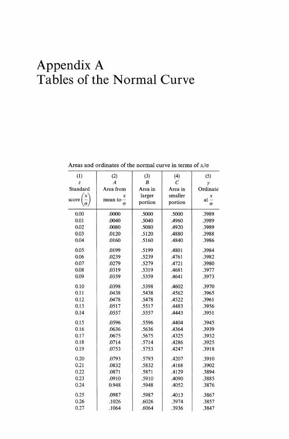
Areas and ordinates of the normal curve in terms of x/cr
(1 ) (2) (3) (4) (5) z A B C Y
Standard Area from Area in Area in Ordinate
score (~) x larger smaller x mean to- portion portion at-
a a
0.00 .0000 .5000 .5000 .3989 0.01 .0040 .5040 .4960 .3989 0.02 .0080 .5080 .4920 .3989 0.G3 .0120 .5120 .4880 .3988 0.04 .0160 .5160 .4840 .3986
0.05 .0199 .5199 .4801 .3984 0.06 .0239 .5239 .4761 .3982 0.07 .0279 .5279 .4721 .3980 0.08 .0319 .5319 .4681 .3977 0.09 .0359 .5359 .4641 .3973
0.10 .0398 .5398 .4602 .3970 0.11 .0438 .5438 .4562 .3965 0.12 .0478 .5478 .4522 .3961 0.13 .0517 .5517 .4483 .3956 0.14 .0557 .5557 .4443 .3951
0.15 .0596 .5596 .4404 .3945 0.16 .0636 .5636 .4364 .3939 0.17 .0675 .5675 .4325 .3932 0.18 .0714 .5714 .4286 .3925 0.19 .0753 .5753 .4247 .3918
0.20 .0793 .5793 .4207 .3910 0.21 .0832 .5832 .4168 .3902 0.22 .0871 .5871 .4129 .3894 0.23 .0910 .5910 .4090 .3885 0.24 0.948 .5948 .4052 .3876
0.25 .0987 .5987 .4013 .3867 0.26 .1026 .6026 .3974 .3857 0.27 .1064 .6064 .3936 .3847

Appendix A. Tables of the Normal Curve 411
(1 ) (2) (3) (4) (5) z A B C Y
Standard Area from Area in Area in Ordinate
score (~) x larger smaller x mean to- portion portion at-
a a
0.28 .1103 .6103 .3897 .3836 0.29 .1141 .6141 .3859 .3825
0.30 .1179 .6179 .3821 .3814 0.31 .1217 .6217 .3783 .3802 0.32 .1255 .6255 .3745 .3790 0.33 .1293 .6293 .3707 .3778 0.34 .1331 .6331 .3669 .3765
0.35 .1368 .6368 .3632 .3752 0.36 .1406 .6406 .3594 .3739 0.37 .1443 .6443 .3557 .3725 0.38 .1480 .6480 .3520 .3712 0.39 .1517 .6517 .3483 .3697
0.40 .1554 .6554 .3446 .3683 0.41 .1591 .6591 .3409 .3668 0.42 .1628 .6628 .3372 .3653 0.43 .1664 .6664 .3336 .3637 0.44 .1700 .6700 .3300 .3621
0.45 .1736 .6736 .3264 .3605 0.46 .1772 .6772 .3228 .3589 0.47 .1808 .6808 .3192 .3572 0.48 .1844 .6844 .3156 .3555 0.49 .1879 .6879 .3121 .3538
0.50 .1915 .6915 .3085 .3521 0.51 .1950 .6950 .3050 .3503 0.52 .1985 .6985 .3015 .3485 0.53 .2019 .7019 .2981 .3467 0.54 .2054 .7054 .2946 .3448
0.55 .2088 .7088 .2912 .3429 0.56 .2123 .7123 .2877 .3410 0.57 .2157 .7157 .2843 .3391 0.58 .2190 .7190 .2810 .3372 0.59 .2224 .7224 .2776 .3352
0.60 .2257 .7257 .2743 .3332 0.61 .2291 .7291 .2709 .3312 0.62 .2324 .7324 .2676 .3292 0.63 .2357 .7357 .2643 .3271 0.64 .2389 .7389 .2611 .3251
0.65 .2422 .7422 .2578 .3230 0.66 .2454 .7454 .2546 .3209 0.67 .2486 .7486 .2514 .3187 0.68 .2517 .7517 .2483 .3166 0.69 .2549 .7549 .2451 .3144
412 Appendix A. Tables of the Normal Curve
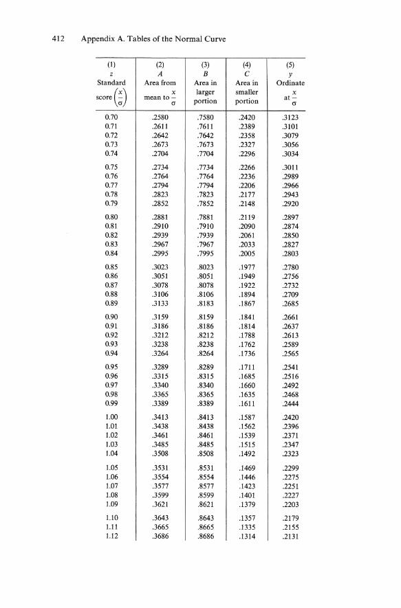
(1) (2) (3) (4) (5) z A B C y
Standard Area from Area in Area in Ordinate
score (~) x larger smaller x mean to- portion portion at
()" ()"
0.70 .2580 .7580 .2420 .3123 0.71 .2611 .7611 .2389 .3101 0.72 .2642 .7642 .2358 .3079 0.73 .2673 .7673 .2327 .3056 0.74 .2704 .7704 .2296 .3034
0.75 .2734 .7734 .2266 .3011 0.76 .2764 .7764 .2236 .2989 0.77 .2794 .7794 .2206 .2966 0.78 .2823 .7823 .2177 .2943 0.79 .2852 .7852 .2148 .2920
0.80 .2881 .7881 .2119 .2897 0.81 .2910 .7910 .2090 .2874 0.82 .2939 .7939 .2061 .2850 0.83 .2967 .7967 .2033 .2827 0.84 .2995 .7995 .2005 .2803
0.85 .3023 .8023 .1977 .2780 0.86 .3051 .8051 .1949 .2756 0.87 .3078 .8078 .1922 .2732 0.88 .3106 .8106 .1894 .2709 0.89 .3133 .8183 .1867 .2685
0.90 .3159 .8159 .1841 .2661 0.91 .3186 .8186 .1814 .2637 0.92 .3212 .8212 .1788 .2613 0.93 .3238 .8238 .1762 .2589 0.94 .3264 .8264 .1736 .2565
0.95 .3289 .8289 .1711 .2541 0.96 .3315 .8315 .1685 .2516 0.97 .3340 .8340 .1660 .2492 0.98 .3365 .8365 .1635 .2468 0.99 .3389 .8389 .1611 .2444
1.00 .3413 .8413 .1587 .2420 1.01 .3438 .8438 .1562 .2396 1.02 .3461 .8461 .1539 .2371 1.03 .3485 .8485 .1515 .2347 1.04 .3508 .8508 .1492 .2323
1.05 .3531 .8531 .1469 .2299 1.06 .3554 .8554 .1446 .2275 1.07 .3577 .8577 .1423 .2251 1.08 .3599 .8599 .1401 .2227 1.09 .3621 .8621 .1379 .2203
1.10 .3643 .8643 .1357 .2179 1.11 .3665 .8665 .1335 .2155 1.12 .3686 .8686 .1314 .2131
Appendix A. Tables of the Normal Curve 413
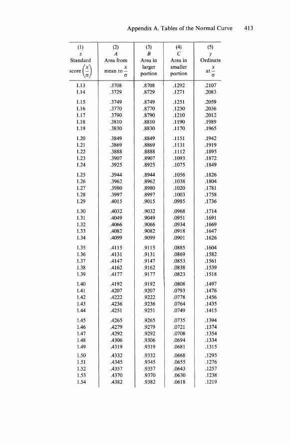
(1 ) (2) (3) (4) (5) z A B C Y
Standard Area from Area in Area in Ordinate
score (~) x larger smaller x mean to- portion portion at-
a a
1.13 .3708 .8708 .1292 .2107 1.14 .3729 .8729 .1271 .2083
1.15 .3749 .8749 .1251 .2059 1.16 .3770 .8770 .1230 .2036 1.17 .3790 .8790 .1210 .2012 1.18 .3810 .8810 .1190 .1989 1.19 .3830 .8830 .1170 .1965
1.20 .3849 .8849 .1151 .1942 1.21 .3869 .8869 .1131 .1919 1.22 .3888 .8888 .1112 .1895 1.23 .3907 .8907 .1093 .1872 1.24 .3925 .8925 .1075 .1849
1.25 .3944 .8944 .1056 .1826 1.26 .3962 .8962 .1038 .1804 1.27 .3980 .8980 .1020 .1781 1.28 .3997 .8997 .1003 .1758 1.29 .4015 .9015 .0985 .1736
1.30 .4032 .9032 .0968 .1714 1.31 .4049 .9049 .0951 .1691 1.32 .4066 .9066 .0934 .1669 1.33 .4082 .9082 .0918 .1647 1.34 .4099 .9099 .0901 .1626
1.35 .4115 .9115 .0885 .1604 1.36 .4131 .9131 .0869 .1582 1.37 .4147 .9147 .0853 .1561 1.38 .4162 .9162 .0838 .1539 1.39 .4177 .9177 .0823 .1518
1.40 .4192 .9192 .0808 .1497 1.41 .4207 .9207 .0793 .1476 1.42 .4222 .9222 .0778 .1456 1.43 .4236 .9236 .0764 .1435 1.44 .4251 .9251 .0749 .1415
1.45 .4265 .9265 .0735 .1394 1.46 .4279 .9279 .0721 .1374 1.47 .4292 .9292 .0708 .1354 1.48 .4306 .9306 .0694 .1334 1.49 .4319 .9319 .0681 .1315
1.50 .4332 .9332 .0668 .1295 1.51 .4345 .9345 .0655 .1276 1.52 .4357 .9357 .0643 .1257 1.53 .4370 .9370 .0630 .1238 1.54 .4382 .9382 .0618 .1219

414 Appendix A. Tables of the Normal Curve
(1 ) (2) (3) (4) (5) z A B C Y
Standard Area from Area in Area in Ordinate
score (;) x larger smaller x
mean to- portion portion at-(J (J
1.55 .4394 .9394 .0606 .1200 1.56 .4406 .9406 .0594 .1182 1.57 .4418 .9418 .0582 .1163 1.58 .4429 .9429 .0571 .1145 1.59 .4441 .9441 .0559 .1127
1.60 .4452 .9452 .0548 .1109 1.61 .4463 .9463 .0537 .1092 1.62 .4474 .9474 .0526 .1074 1.63 .4484 .9484 .0516 .1057 1.64 .4495 .9495 .0505 .1040
1.65 .4505 .9505 .0495 .1023 1.66 .4515 .9515 .0485 .1006 1.67 .4525 .9525 .0475 .0989 1.68 .4535 .9535 .0465 .0973 1.69 .4545 .9545 .0455 .0957
1.70 .4554 .9554 .0446 .0940 1.71 .4564 .9564 .0436 .0925 1.72 .4573 .9573 .0427 .0909 1.73 .4582 .9582 .0418 .0893 1.74 .4591 .9591 .0409 .0878
1.75 .4599 .9599 .0401 .0863 1.76 .4608 .9608 .0392 .0848 1.77 .4616 .9616 .0384 .0833 1.78 .4625 .9625 .0375 .0818 1.79 .4633 .9633 .0367 .0804
1.80 .4641 .9641 .0359 .0790 1.81 .4649 .9649 .0351 .0775 1.82 .4656 .9656 .0344 .0761 1.83 .4664 .9664 .0336 .0748 1.84 .4671 .9671 .0329 .0734
1.85 .4678 .9678 .0322 .0721 1.86 .4686 .9686 .0314 .0707 1.87 .4693 .9693 .0307 .0694 1.88 .4699 .9699 .0301 .0681 1.89 .4706 .9706 .0294 .0669
1.90 .4713 .9713 .0287 .0656 1.91 .4719 .9719 .0281 .0644 1.92 .4726 .9726 .0274 .0632 1.93 .4732 .9732 .0268 .0620 1.94 .4738 .9738 .0262 .0608
1.95 .4744 .9744 .0256 .0596 1.96 .4750 .9750 .0250 .0584 1.97 .4756 .9756 .0244 .0573
Appendix A. Tables of the Normal Curve 415
(1 ) (2) (3) (4) (5) z A B C Y
Standard Area from Area in Area in Ordinate
score (;) x larger smaller x
mean to- portion portion at-IT IT
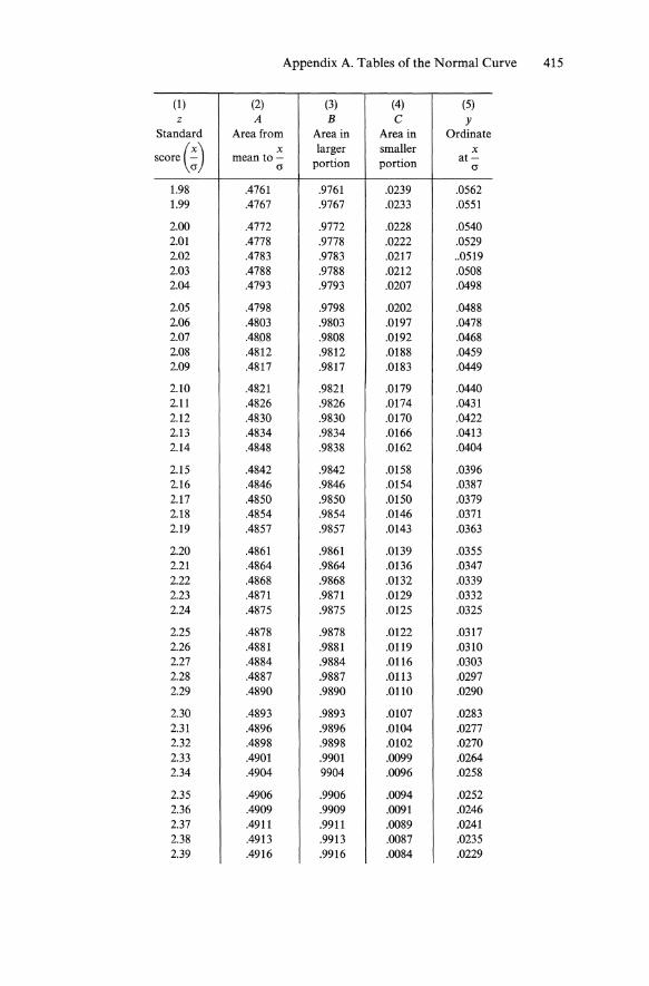
1.98 .4761 .9761 .0239 .0562 1.99 .4767 .9767 .0233 .0551
2.00 .4772 .9772 .0228 .0540 2.01 .4778 .9778 .0222 .0529 2.02 .4783 .9783 .0217 .. 0519 2.03 .4788 .9788 .0212 .0508 2.04 .4793 .9793 .0207 .0498
2.05 .4798 .9798 .0202 .0488 2.06 .4803 .9803 .0197 .0478 2.07 .4808 .9808 .0192 .0468 2.08 .4812 .9812 .0188 .0459 2.09 .4817 .9817 .0183 .0449
2.10 .4821 .9821 .0179 .0440 2.11 .4826 .9826 .0174 .0431 2.12 .4830 .9830 .0170 .0422 2.13 .4834 .9834 .0166 .0413 2.14 .4848 .9838 .0162 .0404
2.15 .4842 .9842 .0158 .0396 2.16 .4846 .9846 .0154 .0387 2.17 .4850 .9850 .0150 .0379 2.18 .4854 .9854 .0146 .0371 2.19 .4857 .9857 .0143 .0363
2.20 .4861 .9861 .0139 .0355 2.21 .4864 .9864 .0136 .0347 2.22 .4868 .9868 .0132 .0339 2.23 .4871 .9871 .0129 .0332 2.24 .4875 .9875 .0125 .0325
2.25 .4878 .9878 .0122 .0317 2.26 .4881 .9881 .0119 .0310 2.27 .4884 .9884 .0116 .0303 2.28 .4887 .9887 .0113 .0297 2.29 .4890 .9890 .0110 .0290
2.30 .4893 .9893 .0107 .0283 2.31 .4896 .9896 .0104 .0277 2.32 .4898 .9898 .0102 .0270 2.33 .4901 .9901 .0099 .0264 2.34 .4904 9904 .0096 .0258
2.35 .4906 .9906 .0094 .0252 2.36 .4909 .9909 .0091 .0246 2.37 .4911 .9911 .0089 .0241 2.38 .4913 .9913 .0087 .0235 2.39 .4916 .9916 .0084 .0229
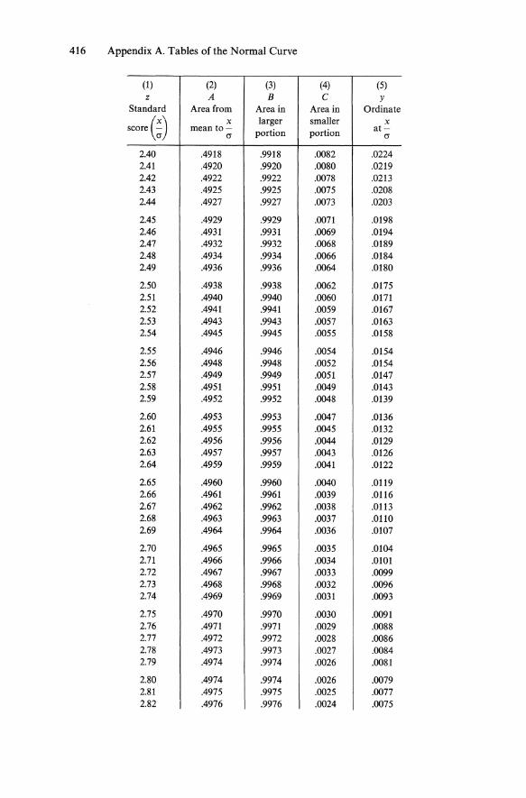
416 Appendix A. Tables of the Normal Curve
(1) (2) (3) (4) (5) z A B C Y
Standard Area from Area in Area in Ordinate
score (~) x larger smaller x mean to- portion portion at-
cr cr
2.40 .4918 .9918 .0082 .0224 2.41 .4920 .9920 .0080 .0219 2.42 .4922 .9922 .0078 .0213 2.43 .4925 .9925 .0075 .0208 2.44 .4927 .9927 .0073 .0203
2.45 .4929 .9929 .0071 .0198 2.46 .4931 .9931 .0069 .0194 2.47 .4932 .9932 .0068 .0189 2.48 .4934 .9934 .0066 .0184 2.49 .4936 .9936 .0064 .0180
2.50 .4938 .9938 .0062 .0175 2.51 .4940 .9940 .0060 .0171 2.52 .4941 .9941 .0059 .0167 2.53 .4943 .9943 .0057 .0163 2.54 .4945 .9945 .0055 .0158
2.55 .4946 .9946 .0054 .0154 2.56 .4948 .9948 .0052 .0154 2.57 .4949 .9949 .0051 .0147 2.58 .4951 .9951 .0049 .0143 2.59 .4952 .9952 .0048 .0139
2.60 .4953 .9953 .0047 .0136 2.61 .4955 .9955 .0045 .0132 2.62 .4956 .9956 .0044 .0129 2.63 .4957 .9957 .0043 .0126 2.64 .4959 .9959 .0041 .0122
2.65 .4960 .9960 .0040 .0119 2.66 .4961 .9961 .0039 .0116 2.67 .4962 .9962 .0038 .0113 2.68 .4963 .9963 .0037 .0110 2.69 .4964 .9964 .0036 .0107
2.70 .4965 .9965 .0035 .0104 2.71 .4966 .9966 .0034 .0101 2.72 .4967 .9967 .0033 .0099 2.73 .4968 .9968 .0032 .0096 2.74 .4969 .9969 .0031 .0093
2.75 .4970 .9970 .0030 .0091 2.76 .4971 .9971 .0029 .0088 2.77 .4972 .9972 .0028 .0086 2.78 .4973 .9973 .0027 .0084 2.79 .4974 .9974 .0026 .0081
2.80 .4974 .9974 .0026 .0079 2.81 .4975 .9975 .0025 .0077 2.82 .4976 .9976 .0024 .0075

Appendix A. Tables ofthe Normal Curve 417
(1) (2) (3) (4) (5) z A B C Y
Standard Area from Area in Area in Ordinate
score (;) x larger smaller x
mean to- portion portion at-cr cr
2.83 .4977 .9977 .0023 .0073 2.84 .4977 .9977 .0023 .0071
2.85 .4978 .9978 .0022 .0069 2.86 .4979 .9979 .0021 .0067 2.87 .4979 .9979 .0021 .0065 2.88 .4980 .9980 .0020 .0063 2.89 .4981 .9981 .0019 .0061
2.90 .4981 .9981 .0019 .0060 2.91 .4982 .9982 .0018 .0058 2.92 .4982 .9982 .0018 .0056 2.93 .4983 .9983 .0017 .0055 2.94 .4984 .9984 .0016 .0053
2.95 .4984 .9984 .0016 .0051 2.96 .4985 .9985 .0015 .0050 2.97 .4985 .9985 .0015 .0048 2.98 .4986 .9986 .0014 .0047 2.99 .4986 .9986 .0014 .0046
3.00 .4987 .9987 .0013 .0044 3.01 .4987 .9987 .0013 .0043 3.02 .4987 .9987 .0013 .0042 3.03 .4988 .9988 .0012 .0040 3.04 .4988 .9988 .0012 .0039
3.05 .4989 .9989 .0011 .0038 3.06 .4989 .9989 .0011 .0037 3.07 .4989 .9989 .0011 .0036 3.08 .4990 .9990 .0010 .0035 3.09 .4990 .9990 .0010 .0034
3.10 .4990 .9990 .0010 .0033 3.11 .4991 .9991 .0009 .0032 3.12 .4991 .9991 .0009 .0031 3.13 .4991 .9991 .0009 .0030 3.14 .4992 .9992 .0008 .0029
3.15 .4992 .9992 .0008 .0028 3.16 .4992 .9992 .0008 .0027 3.17 .4992 .9992 .0008 .0026 3.18 .4993 .9993 .0007 .0025 3.19 .4993 .9993 .0007 .0025
3.20 .4993 .9993 .0007 .0024 3.21 .4993 .9993 .0007 .0023 3.22 .4994 .9994 .0006 .0022 3.23 .4994 .9994 .0006 .0022 3.24 .4994 .9994 .0006 .0021
418 Appendix A. Tables of the Normal Curve
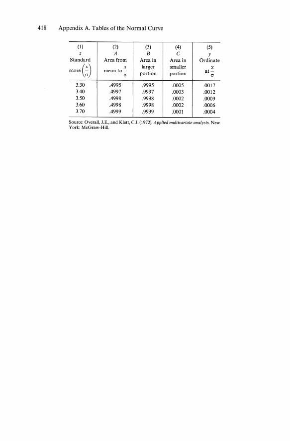
(1) (2) (3) (4) (5) z A B C Y
Standard Area from Area in Area in Ordinate
score (~) x larger smaller x mean to- portion portion at-
cr cr
3.30 .4995 .9995 .0005 .0017 3.40 .4997 .9997 .0003 .0012 3.50 .4998 .9998 .0002 .0009 3.60 .4998 .9998 .0002 .0006 3.70 .4999 .9999 .0001 .0004
Source: Overall, J.E., and Klett, c.J. (1972). Applied multivariate analysis. New York: McGraw-Hill.

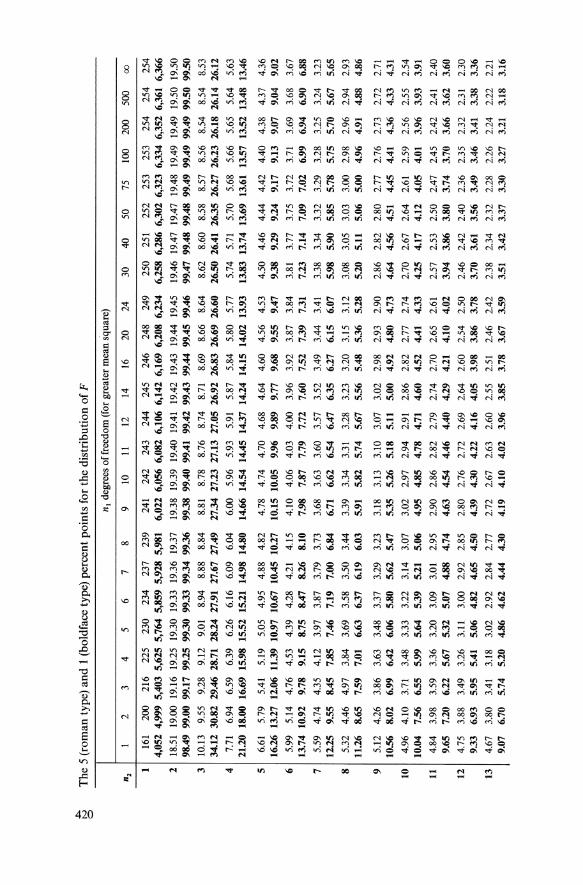
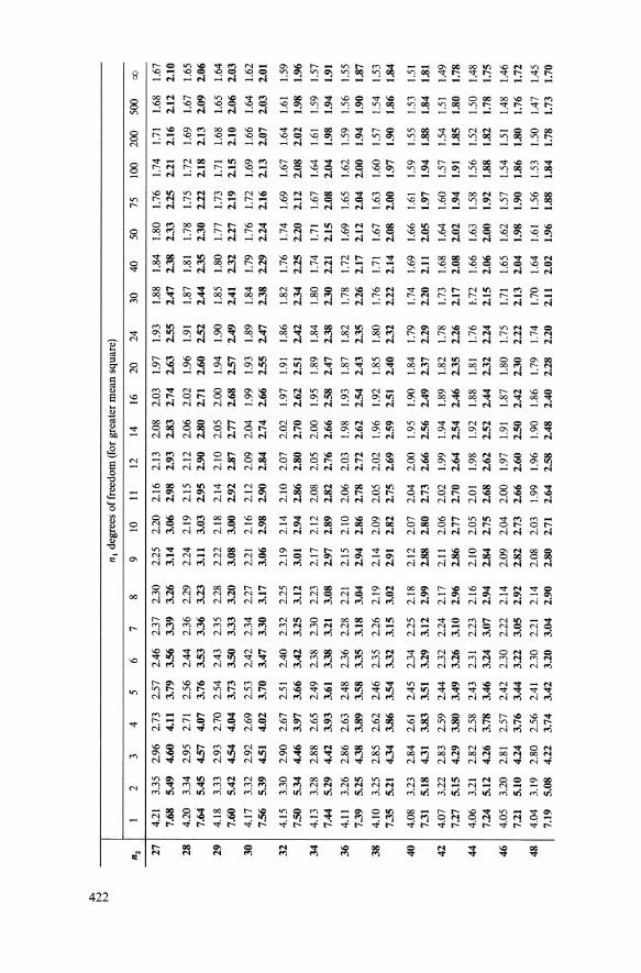
Appendix B Tables of F
~
The
5 (
rom
an ty
pe)
and
1 (b
oldf
ace
type
) pe
rcen
t poi
nts
for
the
dist
ribu
tion
of F
"1 de
gree
s o
f fre
edom
(fo
r gr
eate
r m
ean
squa
re)
"2 1
2 3
4 5
6 7
8 9
10
11
12
14
16
20
24
30
40
50
75
100
200
500
<Xl
161
200
216
225
230
234
237
239
241
242
243
244
245
246
248
249
250
251
252
253
253
254
254
254
4,05
2 4,
999
5,40
3 5,
625
5,76
4 5,
859
5,92
8 5,
981
6,02
2 6,
056
6,08
2 6,
106
6,14
2 6,
169
6,20
8 6,
234
21
18.5
1 19
.00
19.1
6 19
.25
19.3
0 19
.33
19.3
6 19
.37
19.3
8 19
.39
19.4
0 19
.41
19.4
2 19
.43
19.4
4 19
.45
98.4
9 99
.00
99.1
7 99
.25
99.3
0 99
.33
99.3
4 99
.36
99.3
8 99
.40
99.4
1 99
.42
99.4
3 99
.44
99.4
5 99
.46
31
10
.13
9.
55
9.28
9.
12
9.01
8.
94
8.88
8.
84
8.81
8.
78
8.76
8.
74
8.71
8.
69
8.66
8.
64
34.1
2 30
.82
29.4
6 28
.71
28.2
4 27
.91
27.6
7 27
.49
27.3
4 27
.23
27.1
3 27
.05
26.9
2 26
.83
26.6
9 26
.60
6,25
8 6,
286
6,30
2 6,
323
6,33
4 6,
352
6,36
1 6,
366
19.4
6 19
.47
19.4
7 19
.48
19.4
9 19
.49
19.5
0 19
.50
99.4
7 99
.48
99.4
8 99
.49
99.4
9 99
.49
99.5
0 99
.50
8.62
8.
60
8.58
8.
57
8.56
8.
54
8.54
8.
53
26.5
0 26
.41
26.3
5 26
.27
26.2
3 26
.18
26.1
4 26
.12
4 I
7.71
6.
94
6.59
6.
39
6.26
6.
16
6.09
6.
04
6.00
5.
96
5.93
5.
91
5.87
5.
84
5.80
5.
77
5.74
5.
71
5.70
5.
68
5.66
5.
65
5.64
5.
63
21.2
0 18
.00
16.6
9 15
.98
15.5
2 15
.21
14.9
8 14
.80
14.6
6 14
.54
14.4
5 14
.37
14.2
4 14
.]5
]4.0
2 13
.93
13.8
3 13
.74
13.6
9 13
.61
13.5
7 13
.52
13.4
8 13
.46
5 I
6.61
5.
79
5.41
5.
19
5.05
4.
95
4.88
4.
82
4.78
4.
74
4.70
4.
68
4.64
4.
60
4.56
4.
53
4.50
4.
46
4.44
4.
42
4.40
4.
38
4.37
4.
36
16.2
6 13
.27
12.0
6 11
.39
10.9
7 10
.67
10.4
5 10
.27
10.1
5 10
.05
9.96
9.
89
9.77
9.
68
9.55
9.
47
9.38
9.
29
9.24
9.
17
9.13
9.
07
9.04
9.
02
61
5.99
5.
14
4.76
4.
53
4.39
4.
28
4.21
4.
15
4.10
4.
06
4.03
4.
00
3.96
3.
92
3.87
3.
84
3.81
3.
77
3.75
3.
72
3.71
3.
69
3.68
3.
67
13.7
4 10
.92
9.78
9.
15
8.75
8.
47
8.26
8.
10
7.98
7.
87
7.79
7.
72
7.60
7.
52
7.39
7.
31
7.23
7.
14
7.09
7.
02
6.99
6.
94
6.90
6.
88
71
5.59
4.
74
4.35
4.
12
3.97
3.
87
3.79
3.
73
3.68
3.
63
3.60
3.
57
3.52
3.
49
3.44
3.
41
3.38
3.
34
3.32
3.
29
3.28
3.
25
3.24
3.
23
12.2
5 9.
55
8.45
7.
85
7.46
7.
19
7.00
6.
84
6.71
6.
62
6.54
6.
47
6.35
6.
27
6.15
6.
07
5.98
5.
90
5.85
5.
78
5.75
5.
70
5.67
5.
65
8 I
5.32
4.
46
4.97
3.
84
3.69
3.
58
3.50
3.
44
3.39
3.
34
3.31
3.
28
3.23
3.
20
3.15
3.
12
11.2
6 8.
65
7.59
7.
01
6.63
6.
37
6.19
6.
03
5.91
5.
82
5.74
5.
67
5.56
5.
48
5.36
5.
28
91
5.12
4.
26
3.86
3.
63
3.48
3.
37
3.29
3.
23
3.18
3.
13
3.10
3.
07
3.02
2.
98
2.93
2.
90
10.5
6 8.
02
6.99
6.
42
6.06
5.
80
5.62
5.
47
5.35
5.
26
5.18
5.
11
5.00
4.
92
4.80
4.
73
10 1
4.
96
4.10
3.
71
3.48
3.
33
3.22
3.
14
3.07
3.
02
2.97
2.
94
2.91
2.
86
2.82
2.
77
2.74
10
.04
7.56
6.
55
5.99
5.
64
5.39
5.
21
5.06
4.
95
4.85
4.
78
4.71
4.
60
4.52
4.
41
4.33
11 1
4.
84
3.98
3.
59
3.36
3.
20
3.09
3.
01
2.95
2.
90
2.86
2.
82
2.79
2.
74
2.70
2.
65
2.61
9.
65
7.20
6.
22
5.67
5.
32
5.07
4.
88
4.74
4.
63
4.54
4.
46
4.40
4.
29
4.21
4.
10
4.02
121
4.75
3.
88
3.49
3.
26
3.11
3.
00
2.92
2.
85
2.80
2.
76
2.72
2.
69
2.64
2.
60
2.54
2.
50
9.33
6.
93
5.95
5.
41
5.06
4.
82
4.65
4.
50
4.39
4.
30
4.22
4.
16
4.05
3.
98
3.86
3.
78
131
4.67
3.
80
3.41
3.
18
3.02
2.
92
2.84
2.
77
2.72
2.
67
2.63
2.
60
2.55
2.
51
2.46
2.
42
9.07
6.
70
5.74
5.
20
4.86
4.
62
4.44
4.
30
4.19
4.
10
4.02
3.
96
3.85
3.
78
3.67
3.
59
3.08
3.
05
3.03
3.
00
2.98
2.
96
2.94
2.
93
5.20
5.
11
5.06
5.
00
4.96
4.
91
4.88
4.
86
2.86
2.
82
2.80
2.
77
2.76
2.
73
2.72
2.
71
4.64
4.
56
4.51
4.
45
4.41
4.
36
4.33
4.
31
2.70
2.
67
2.64
2.
61
2.59
2.
56
2.55
2.
54
4.25
4.
17
4.12
4.
05
4.01
3.
96
3.93
3.
91
2.57
2.
53
2.50
2.
47
2.45
2.
42
2.41
2.
40
3.94
3.
86
3.80
3.
74
3.70
3.
66
3.62
3.
60
2.46
2.
42
2.40
2.
36
2.35
2.
32
2.31
2.
30
3.70
3.
61
3.56
3.
49
3.46
3.
41
3.38
3.
36
2.38
2.
34
2.32
2.
28
2.26
2.
24
2.22
2.
21
3.51
3.
42
3.37
3.
30
3.27
3.
21
3.18
3.
16
"" tv ....
14 I
4.60
3.
74
3.34
3.
11
2.96
2.
85
2.77
2.
70
2.65
2.
60
2.56
2.
53
2.48
2.
44
2.39
2.
35
2.31
2.
27
2.24
2.
21
2.19
2.
16
2.14
2.
13
8.86
6.
51
5.56
5.
03
4.69
4.
46
4.28
4.
14
4.03
3.
94
3.86
3.
80
3.70
3.
62
3.51
3.
43
3.34
3.
26
3.21
3.
14
3.11
3.
06
3.02
3.
00
15 I
4.
54
3.68
3.
29
3.06
2.
90
2.79
2.
70
2.64
2.
59
2.55
2.
51
2.48
2.
43
2.39
2.
33
2.29
2.
25
2.21
2.
18
2.15
2.
12
2.10
2.
08
2.07
~~~~~~~~~~~~~~~~~~~~~~~~
16 I
4.49
3.
63
3.24
3.
01
2.85
2.
74
2.66
2.
59
2.54
2.
49
2.45
2.
42
2.37
2.
33
2.28
2.
24
2.20
2.
16
2.13
2.
09
2.07
2.
04
2.02
2.
01
~~~~~~~~~~~~~~~~~~~~~~~~
17 I
4.
45
3.59
3.
20
2.96
2.
81
2.70
2.
62
2.55
2.
50
2.45
2.
41
2.38
2.
33
2.29
2.
23
2.19
2.
15
2.11
2.
08
2.04
2.
02
1.99
1.
97
1.96
8.
40
6.11
5.
18
4.67
4.
34
4.10
3.
93
3.79
3.
68
3.59
3.
52
3.45
3.
35
3.27
3.
16
3.08
3.
00
2.92
2.
86
2.79
2.
76
2.70
2.
67
2.65
18 I
4.41
3.
55
3.16
2.
93
2.77
2.
66
2.58
2.
51
8.28
6.
01
5.09
4.
58
4.25
4.
01
3.85
3.
71
19 I
4.38
3.
52
3.13
2.
90
274
263
2.55
2.
48
8.18
5.
93
5.01
4.
50
4.17
3.
94
3.77
3.
63
2.46
2.
41
2.37
2.
34
2.29
2.
25
2.19
2.
15
3.60
3.
51
3.44
3.
37
3.27
3.
19
3.07
3.
00
2.43
2.
38
2.34
2.
31
2.26
2.
21
2.15
2.
11
3.52
3.
43
3.36
3.
10
3.19
3.
12
3.00
2.
92
2.11
2.
07
2.04
2.
00
1.98
1.
95
1.93
1.
92
2.91
2.
83
2.78
2.
71
2.68
2.
62
2.59
2.
57
2.07
20
2 20
0 1.
96
1.94
1.
91
1.90
1.
88
2.84
2.
76
2.70
2.
63
2.60
2.
54
2.51
2.
49
20 I
4.
35
3.49
3.
10
2.87
2.
71
2.60
2.
52
2.45
2.
40
2.35
2.
31
2.28
2.
23
2.18
2.
12
2.08
2.
04
1.99
1.
96
1.92
1.
90
1.87
1.
85
1.84
8.
10
5.85
4.
94
4.43
4.
10
3.87
3.
71
3.56
3.
45
3.37
3.
30
3.23
3.
13
3.05
2.
94
2.86
2.
77
2.69
2.
63
2.S6
2.
53
2.47
2.
44
2.42
21 I
4.
32
3.47
3.
07
2.84
2.
68
2.57
2.
49
2.42
2.
37
2.32
2.
28
2.25
2.
20
2.15
2.
09
2.05
2.
00
1.96
1.
93
1.89
1.
87
1.84
1.
82
1.81
~~~~~W~~~~~~~~~~~~~~~~~~
22 I
4.
30
3.44
3.
05
2.82
2.
66
2.55
2.
47
2.40
2.
35
2.30
2.
26
2.23
2.
18
2.13
2.
07
2.03
1.
98
1.93
1.
91
1.87
1.
84
L81
L80
1.
78
~~~~~~~~~~~~~~~~~~~~~~~~
23 I
4.28
3.
42
3.03
2.
80
2.64
2.
53
2.45
2.
38
2.32
2.
28
2.24
2.
20
2.14
2.
10
2.04
2.
00
1.96
1.
91
1.88
1.
84
1.82
1.
79
1.77
1.
76
~~~~~~~~~m~~~~~~~~~~~~~~
24 I
4.
26
3.40
3.
01
2.78
2.
62
2.51
2.
43
2.36
2.
30
2.26
2.
22
2.18
2.
13
2.09
20
2 1.
98
1.94
1.
89
1.86
1.
82
1.80
1.
76
1.74
1.
73
~~~~~~~~~~~~~~~~~~~~~~~~
25 I
4.2
4 3.
38
2.99
2.
76
2.60
2.
49
2.41
2.
34
7.77
5.
57
4.68
4.
18
3.86
3.
63
3.46
3;
32
26 I
4.22
3.
37
2.98
2.
74
2.59
2.
47
2.39
2.
32
7.72
5.
53
4.64
4.
14
3.82
3.
59
3.42
3.
29
2.28
2.
24
2.20
2.
16
2.11
2.
06
2.00
1.
96
3.21
3.
13
3.05
2.
99
2.89
2.
81
2.70
2.
62
2.27
2.
22
2.18
2.
15
2.10
2.
05
1.99
1.
95
3.17
3.
09
3.02
2.
96 ~
2.77
2.
66 ~
1.92
1.
87
1.84
1.
80
1.77
1.
74
1.72
1.
71
2.S4
2.
45
2.40
2.
32
2.29
~
2.19
2.
17
1.90
1.
85
1.82
1.
78
1.76
1.
72
1.70
1.
69
2.SO
2.41
2.
36
2.28
2.
25
2.19
2.
15
2.13
.l>
N
N
n z
2 3
4 5
6 7
8
271
4.21
3.
35
2.96
2.
73
2.57
2.
46
2.37
2.
30
7.68
5.
49
4.60
4.
11
3.79
3.
56
3.39
3.
26
28
4.20
3.
34
2.95
2.
71
2.56
2.
44
2.36
2.
29
7.64
5.
45
4.57
4.
07
3.76
3.
53
3.36
3.
23
29
4.18
3.
33
2.93
2.
70
2.54
2.
43
2.35
2.
28
7.60
5.
42
4.54
4.
04
3.73
3.
50
3.33
3.
20
30
4.17
3.
32
2.92
2.
69
2.53
2.
42
2.34
2.
27
7.56
5.
39
4.51
4.
02
3.70
3.
47
3.30
3.
17
32
4.15
3.
30
2.90
2.
67
2.51
2.
40
2.32
2.
25
7.50
5.
34
4.46
3.
97
3.66
3.
42
3.25
3.
12
34
4.13
3.
28
2.88
2.
65
2.49
2.
38
2.30
2.
23
7.44
5.
29
4.42
3.
93
3.61
3.
38
3.21
3.
08
361
4.11
3.
26
2.86
2.
63
2.48
2.
36
2.28
2.
21
7.39
5.
25
4.38
3.
89
3.58
3.
35
3.18
3.
04
38 I
4.
10
3.25
2.
85
2.62
2.
46
2.35
2.
26
2.19
7.
35
5.21
4.
34
3.86
3.
54
3.32
3.
15
3.02
40
4.08
3.
23
2.84
2.
61
2.45
2.
34
2.25
2.
18
7.31
5.
18
4.31
3.
83
3.51
3.
29
3.12
2.
99
42
4.07
3.
22
2.83
2.
59
2.44
2.
32
2.24
2.
17
7.27
5.
15
4.29
3.
80
3.49
3.
26
3.10
2.
96
44 I
4.06
3.
21
2.82
2.
58
2.43
2.
31
2.23
2.
16
7.24
5.
12
4.26
3.
78
3.46
3.
24
3.07
2.
94
46
4.05
3.
20
2.81
2.
57
2.42
2.
30
2.22
2.
14
7.21
5.
10
4.24
3.
76
3.44
3.
22
3.05
2.
92
48
4.04
3.
19
2.80
2.
56
2.41
2.
30
2.21
2.
14
7.19
5.
08
4.22
3.
74
3.42
3.
20
3.04
2.
90
n, d
egre
es o
f fre
edom
(fo
r gr
eate
r m
ean
squa
re)
9 10
11
12
14
16
20
24
2.25
2.
20
2.16
2.
13
2.08
2.
03
1.97
1.
93
3.14
3.
06
2.98
2.
93
2.83
2.
74
2.63
2.
55
2.24
2.
19
2.15
2.
12
2.06
2.
02
1.96
1.
91
3.11
3.
03
2.95
2.
90
2.80
2.
71
2.60
2.
52
2.22
2.
18
2.14
2.
10
2.05
2.
00
1.94
1.
90
3.08
3.
00
2.92
2.
87
2.77
2.
68
2.57
2.
49
2.21
2.
16
2.12
2.
09
2.04
1.
99
1.93
1.
89
3.06
2.
98
2.90
2.
84
2.74
2.
66
2.55
2.
47
2.19
2.
14
2.10
2.
07
2.02
1.
97
1.91
1.
86
3.01
2.
94
2.86
2.
80
2.70
2.
62
2.51
2.
42
2.17
2.
12
2.08
2.
05
2.00
1.
95
1.89
1.
84
2.97
2.
89
2.82
2.
76
2.66
2.
58
2.47
2.
38
2.15
2.
10
2.06
2.
03
1.98
1.
93
1.87
1.
82
2.94
2.
86
2.78
2.
72
2.62
2.
54
2.43
2.
35
2.14
2.
09
2.05
2.
02
1.96
1.
92
1.85
1.
80
2.91
2.
82
2.75
2.
69
2.59
2.
51
2.40
2.
32
2.12
2.
07
2.04
2.
00
1.95
1.
90
1.84
1.
79
2.88
2.
80
2.73
2.
66
2.56
2.
49
2.37
2.
29
2.11
2.
06
2.02
1.
99
1.94
1.
89
1.82
1.
78
2.86
2.
77
2.70
2.
64
2.54
2.
46
2.35
2.
26
2.10
2.
05
2.01
1.
98
1.92
1.
88
1.81
1.
76
2.84
2.
75
2.68
2.
62
2.52
2.
44
2.32
2.
24
2.09
2.
04
2.00
1.
97
1.91
1.
87
1.80
1.
75
2.82
2.
73
2.66
2.
60
2.50
2.
42
2.30
2.
22
2.08
2.
03
1.99
1.
96
1.90
1.
86
1.79
1.
74
2.80
2.
71
2.64
2.
58
2.48
2.
40
2.28
2.
20
30
40
50
75
100
200
500
rxJ
1.88
1.
84
1.80
1.
76
1.74
1.
71
1.68
1.
67
2.47
2.
38
2.33
2.
25
2.21
2.
16
2.12
2.
10
1.87
1.
81
1.78
1.
75
1. 72
1.
69
1.67
1.
65
2.44
2.
35
2.30
2.
22
2.18
2.
13
2.09
2.
06
1.85
1.
80
1.77
1.
73
1.71
1.
68
1.65
1.
64
2.41
2.
32
2.27
2.
19
2.15
2.
10
2.06
2.
03
1.84
1.
79
1.76
1.
72
1.69
1.
66
1.64
1.
62
2.38
2.
29
2.24
2.
16
2.13
2.
07
2.03
2.
01
1.82
1.
76
1.74
1.
69
1.67
1.
64
1.61
1.
59
2.34
2.
25
2.20
2.
12
2.08
2.
02
1.98
1.
96
1.80
1.
74
1.71
1.
67
1.64
1.
61
1.59
1.
57
2.30
2.
21
2.15
2.
08
2.04
1.
98
1.94
1.
91
1.78
1.
72
1.69
1.
65
1.62
1.
59
1.56
1.
55
2.26
2.
17
2.12
2.
04
2.00
1.
94
1.90
1.
87
1.76
1.
71
1.67
1.
63
1.60
1.
57
1.54
1.
53
2.22
2.
14
2.08
2.
00
1.97
1.
90
1.86
1.
84
1.74
1.
69
1.66
1.
61
1.59
1.
55
1.53
1.
51
2.20
2.
11
2.05
1.
97
1.94
1.
88
1.84
1.
81
1.73
1.
68
1.64
1.
60
1.57
1.
54
1.51
1.
49
2.17
2.
08
2.02
1.
94
1.91
1.
85
1.80
1.
78
1. 72
1.
66
1.63
1.
58
1.56
1.
52
1.50
1.
48
2.15
2.
06
2.00
1.
92
1.88
1.
82
1.78
1.
75
1.71
1.
65
1.62
1.
57
1.54
1.
51
1.48
1.
46
2.13
2.
04
1.98
1.
90
1.86
1.
80
1.76
1.
72
1.70
1.
64
1.61
1.
56
1.53
1.
50
1.47
1.
45
2.11
2.
02
1.96
1.
88
1.84
1.
78
1.73
1.
70

+:>.
N
w
50 I
4.
03
3.18
2.
79
2.56
2.
40
2.29
2.
20
2.13
7.
17
5.06
4.
20
3.72
3.
41
3.18
3.
02
2.88
55 I
4.02
3.
17
2.78
2
54
2.
38
2.27
2.
18
2.11
7.
12
5.01
4.
16
3.68
3.
37
3.15
2.
98
2.85
60
4.00
3.
15
2.76
2.
52
2.37
2.
25
2.17
2.
10
7.08
4.
98
4.13
3.
65
3.34
3.
12
2.95
2.
82
65
3.99
3.
14
2.75
2.
51
2.36
2.
24
2.15
2.
08
7.04
4.
95
4.10
3.
62
3.31
3.
09
2.93
2.
79
70 I
3.98
3.
13
2.74
2.
50
2.35
2.
23
2.14
2.
07
7.01
4.
92
4.08
3.
60
3.29
3.
07
2.91
2.
77
80 I
3.96
3.
11
2.72
2.
48
2.33
2.
21
2.12
2.
05
6.96
4.
88
4.04
3.
56
3.25
3.
04
2.87
2.
74
100
I 3.
94
3.09
2.
70
2.46
2.
30
2.19
2.
10
2.03
6.
90
4.82
3.
98
3.51
3.
20
2.99
2.
82
2.69
125 I
3.92
3.
07
2.68
2.
44
2.29
2.
17
2.08
2.
01
6.84
4.
78
3.94
3.
47
3.17
2.
95
2.79
2.
65
150
3.91
3.
06
2.67
2.
43
2.27
2.
16
2.07
2.
00
6.81
4.
75
3.91
3.
44
3.14
2.
92
2.76
2.
62
200
3.89
3.
04
2.65
2.
41
2.26
2.
14
2.05
1.
98
6.76
4.
71
3.88
3.
41
3.11
2.
90
2.73
2.
60
400
3.86
3.
02
2.62
2.
39
2.23
2.
12
2.03
1.
96
6.70
4.
66
3.83
3.
36
3.06
2.
85
2.69
2.
55
1000
I 3.
85
3.00
2.
61
2.38
2.
22
2.10
2.
02
1.95
6.
66
4.62
3.
80
3.34
3.
04
2.82
2.
66
2.53
OCJ
I 3.
84
2.99
2.
60
2.37
2.
21
2.09
2.
01
1.94
6.
64
4.60
3.
78
3.32
3.
02
2.80
2.
64
2.51
2.07
2.
02
1.98
1.
95
1.90
1.
85
1.78
1.
74
2.78
2.
70
2.62
2.
56
2.46
2.
39
2.26
2.
18
2.05
2.
00
1.97
1.
93
1.88
1.
83
1.76
1.
72
2.75
2.
66
2.59
2.
53
2.43
2.
35
2.23
2.
15
2.04
1.
99
1.95
1.
92
1.86
1.
81
1.75
1.
70
2.72
2.
63
2.56
2.
50
2.40
2.
32
2.20
2.
12
2.02
1.
98
1.94
1.
90
1.85
1.
80
1.73
1.
68
2.70
2.
61
2.54
2.
47
2.37
2.
39
2.18
2.
09
2.01
1.
07
1.93
1.
89
1.84
1.
79
1.72
1.
67
2.67
2.
59
2.51
2.
45
2.35
2.
28
2.15
2.
07
1.99
1.
95
1.91
1.
88
1.82
1.
77
1.70
1.
65
2.64
2.
55
2.48
2.
41
2.32
2.
24
2.11
2.
03
1.97
1.
92
1.88
1.
85
1.79
1.
75
1.68
1.
63
2.59
2.
51
2.43
2.
36
2.26
2.
19
2.06
1.
98
1.95
1.
90
1.86
1.
83
1.77
1.
72
1.65
1.
60
2.56
2.
47
2.40
2.
33
2.23
2.
15
2.03
1.
94
1.94
1.
89
1.85
1.
82
1.76
1.
71
1.64
1.
59
2.53
2.
44
2.37
2.
30
2.20
2.
12
2.00
1.
91
1.92
1.
87
1.83
1.
80
1.74
1.
69
1.62
1.
57
2.50
2.
41
2.34
2.
28
2.17
2.
09
1.97
1.
88
1.90
1.
85
1.81
1.
78
1.72
1.
67
1.60
1.
54
2.46
2.
37
2.29
2.
23
2.12
2.
04
1.92
1.
84
1.89
1.
84
1.80
1.
76
1.70
1.
65
1.58
1.
53
2.43
2.
34
2.26
2.
20
2.09
2.
01
1.89
1.
81
1.88
1.
83
1.79
1.
75
1.69
1.
64
1.57
1.
52
2.41
2.
32
2.24
2.
18
2.07
1.
99
1.87
1.
79
1.69
1.
63
1.60
1.
55
1.52
1.
48
1.46
1.
44
2.10
2.
00
1.94
1.
86
1.82
1.
76
1.71
1.
68
1.67
1.
61
1.58
1.
52
1.50
1.
46
1.43
1.
41
2.06
1.
96
1.90
1.
82
1.78
1.
71
1.66
1.
64
1.65
1.
59
1.56
1.
50
1.48
1.
44
1.41
1.
39
2.03
1.
93
1.87
1.
79
1.74
1.
68
1.63
1.
60
1.63
1.
57
1.54
1.
49
1.46
1.
42
1.39
1.
37
2.00
1.
90
1.84
1.
76
1.71
1.
64
1.60
1.
56
1.62
1.
56
1.53
1.
47
1.45
1.
40
1.37
1.
35
1.98
1.
88
1.82
1.
74
1.69
1.
62
1.56
1.
53
1.60
1.
54
1.51
1.
45
1.42
1.
38
1.35
1.
32
1.94
1.
84
1.78
1.
70
1.65
1.
57
1.52
1.
49
1.57
1.
51
1.48
1.
42
1.39
1.
34
1.30
1.
28
1.89
1.
79
1.73
1.
64
1.59
1.
51
1.46
1.
43
1.55
1.
49
1.45
1.
39
1.36
1.
31
1.27
1.
25
1.85
1.
75
1.68
1.
59
1.54
1.
46
1.40
1.
37
1.54
1.
47
1.44
1.
37
1.34
1.
29
1.25
1.
22
1.83
1.
72
1.66
1.
56
1.51
1.
43
1.37
1.
33
1.52
1.
45
1.42
1.
35
1.32
1.
26
1.22
1.
19
1.79
1.
69
1.62
1.
53
1.48
1.
39
1.33
1.
28
1.49
1.
42
1.38
1.
32
1.28
1.
22
1.16
1.
13
1.74
1.
64
1.57
1.
47
1.42
1.
32
1.24
1.
19
1.47
1.
41
1.36
1.
30
1.26
1.
19
1.13
1.
08
1.71
1.
61
1.54
1.
44
1.38
1.
28
1.19
1.
11
1.46
1.
40
1.35
1.
28
1.24
1.
17
1.11
1.
00
1.69
1.
59
1.52
1.
41
1.36
1.
25
1.15
1.
00
Sour
ce:
Rep
rint
ed b
y pe
rmis
sion
fro
m S
TA
TIS
TIC
AL
ME
TH
OD
S, S
even
th E
diti
on b
y G
eorg
e W
. S
nede
cor
and
Wil
liam
G.
Coc
hran
© 1
980
by I
owa
Sta
te U
nive
rsit
y Pr
ess,
212
1 S
outh
S
tate
Ave
., A
mes
, Iow
a 50
010.

Upp
er p
erce
ntag
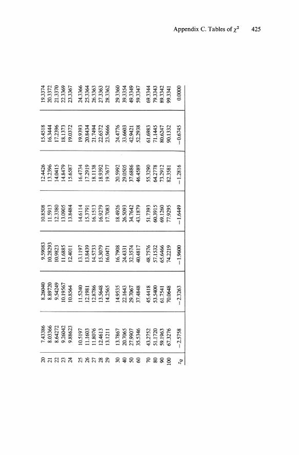
e po
ints
of t
he X
2 di
stri
buti
on
~
0.99
5 0.
990
.097
5 0.
950
1 39
2704
.10-
10
15
7088
.lO
-9
9820
69.l
O-9
39
3214
.10-
8
2 0.
0100
251
0.02
0100
7 0.
0506
356
0.lO
2587
3
0.07
1721
2 0.
1148
32
0.21
5795
0.
3518
46
4 0.
2069
90
0.29
7110
0.
4844
19
0.7l
O72
1
5 0.
4117
40
0.55
4300
0.
8312
11
1.14
5476
6
0.67
5727
0.
8720
85
1.23
7347
1.
6353
9 7
0.98
9265
1.
2390
43
1.68
987
2.16
735
8 1.
3444
19
1.64
6482
2.
1797
3 2.
7326
4 9
1.73
4926
2.
0879
12
2.70
039
3.32
511
lO
2.15
585
2.55
821
3.24
697
3.94
030
11
2.60
321
3.05
347
3.81
575
4.57
481
12
3.07
382
3.57
056
4.40
379
5.22
603
13
3.56
503
4.lO
691
5.00
874
5.89
186
14
4.07
468
4.66
043
5.62
872
6.57
063
15
4.60
094
5.22
935
6.26
214
7.26
094
16
5.14
224
5.81
221
6.90
766
7.96
164
17
5.69
724
6.40
776
7.56
418
8.67
176
18
6.26
481
7.01
491
8.23
075
9.39
046
19
6.84
398
7.63
273
8.90
655
lO.1
170
0.90
0 0.
750
0.01
5790
8 0.
1015
308
0.21
0720
0.
5753
64
0.58
4375
1.
2125
34
1.06
3623
1.
9225
5
1.6l
O31
2.
6746
0 2.
2041
3 3.
4546
0 2.
8331
1 4.
2548
5 3.
4895
4 5.
0706
4 4.
1681
6 5.
8988
3
4.86
518
6.73
720
5.57
779
7.58
412
6.30
380
8.43
842
7.04
150
9.29
906
7.78
953
lO.1
653
8.54
675
11.0
365
9.31
223
11.9
122
lO.0
852
12.7
919
10.8
649
13.6
753
11.6
509
14.5
620
0.50
0
0.45
4937
1.
3862
9 2.
3659
7 3.
3567
0
4.35
146
5.34
812
6.34
581
7.34
412
8.34
283
9.34
182
10.3
4lO
11
.340
3 12
.339
8 13
.339
3
14.3
389
15.3
385
16.3
381
17.3
379
18.3
376
~>
~~
cJ~
~(t)
(t)
::i
00
0..
o
1-0<
' ~~
~Nn
20
7.43
386
8.26
040
9.59
083
10.8
508
12.4
426
15.4
518
19.3
374
21
8.03
366
8.89
720
10.2
8293
11
.591
3 13
.239
6 16
.344
4 20
.337
2
22
8.64
272
9.54
249
10.9
823
12.3
380
14.0
415
17.2
396
21.3
370
23
9.26
042
10.1
9567
11
.688
5 13
.090
5 14
.847
9 18
.137
3 22
.336
9
24
9.88
623
10.8
564
12.4
011
13.8
484
15.6
587
19.0
372
23.3
367
25
10.5
197
11.5
240
13.1
197
14.6
114
16.4
734
19.9
393
24.3
366
26
11.1
603
12.1
981
13.8
439
15.3
791
17.2
919
20.8
434
25.3
364
27
11.8
076
12.8
786
14.5
733
16.1
513
18.1
138
21.7
494
26.3
363
28
12.4
613
13.5
648
15.3
079
16.9
279
18.9
392
22.6
572
27.3
363
29
13.1
211
14.2
565
16.0
471
17.7
083
19.7
677
23.5
666
28.3
362
30
13.7
867
14.9
535
16.7
908
18.4
926
20.5
992
24.4
776
29.3
360
40
20.7
065
22.1
643
24.4
331
26.5
093
29.0
505
33.6
603
39.3
354
50
27.9
907
29.7
067
32.3
574
34.7
642
37.6
886
42.9
421
49.3
349
60
35.5
346
37.4
848
40.4
817
43.1
879
46.4
589
52.2
938
59.3
347
70
43.2
752
45.4
418
48.7
576
51.7
393
55.3
290
61.6
983
69.3
344
80
51.1
720
53.5
400
57.1
532
60.3
915
64.2
778
71.1
445
79.3
343
90
59.1
963
61.7
541
65.6
466
69.1
260
73.2
912
80.6
247
89.3
342
100
67.3
276
70.0
648
74.2
219
77.9
295
82.3
581
90.1
332
99.3
341
-2.5
75
8
-2.3
26
3
-1.9
60
0
-1.6
44
9
-1.2
81
6
-0.6
74
5
0.00
00
;J>
ZQ
'0
-g >:l
0.
. s:;.
(1
>-l
!lJ
cr" <>
til 0 -.
~ '" """ IV
VI

~
0.25
0 0.
100
0.05
0
1 1.
3233
0 2.
7055
4 3.
8414
6 2
2.77
259
4.60
517
5.99
147
3 4.
1083
5 6.
2513
9 7.
8147
3 4
5.38
527
7.77
944
9.48
773
5 6.
6256
8 9.
2363
5 11
.070
5 6
7.84
080
10.6
446
12.5
916
7 9.
0371
5 12
.017
0 14
.067
1 8
10.2
188
13.3
616
15.5
073
9 11
.388
7 14
.683
7 16
.919
0
10
12.5
489
15.9
871
18.3
070
11
13.7
007
17.2
750
19.6
751
12
14.8
454
18.5
494
21.0
261
13
15.9
839
19.8
119
22.3
621
14
17.1
170
21.0
642
23.6
848
15
18.2
451
22.3
072
24.9
958
16
19.3
688
23.5
418
26.2
962
17
20.4
887
24.7
690
27.5
871
18
21.6
049
25.9
894
28.8
693
19
22.7
178
27.2
036
30.1
435
0.Q
25
0.01
0
5.02
389
6.63
490
7.37
776
9.21
034
9.34
840
11.3
449
11.1
433
13.2
767
12.8
325
15.0
863
14.4
494
16.8
119
16.0
128
18.4
753
17.5
346
20.0
902
19.0
228
21.6
660
20.4
831
23.2
093
21.9
200
24.7
250
23.3
367
26.2
170
24.7
356
27.6
883
26.1
190
29.1
413
27.4
884
30.5
779
28.8
454
31.9
999
30.1
910
33.4
087
31.5
264
34.8
053
32.8
532
36.1
908
0.00
5
7.87
944
10.5
966
12.8
381
14.8
602
16.7
496
18.5
476
20.2
777
21.9
550
23.5
893
25.1
882
26.7
569
28.2
995
29.8
194
31.3
193
32.8
013
34.2
672
35.7
185
37.1
564
38.5
822
0.00
1
10.8
28
13.8
16
16.2
66
18.4
67
20.5
15
22.4
58
24.3
22
26.1
25
27.8
77
29.5
88
31.2
64
32.9
09
34.5
28
36.1
23
37.6
97
39.2
52
40.7
90
42.3
12
43.8
20
.l>
N
0\ >
~ :::: 0.
~.
(1
>-l ~
~
en
o -.
~ '"

20
23.8
277
28.4
120
31.4
104
34.1
696
37.5
662
39.9
968
45.3
15
21
24.9
348
29.6
151
32.6
705
35.4
789
38.9
321
41.4
010
46.7
97
22
26.0
393
30.8
133
33.9
244
36.7
807
40.2
894
42.7
956
48.2
68
23
27.1
413
32.0
069
35.1
725
38.0
757
41.6
384
44.1
813
49.7
28
24
28.2
412
33.1
963
36.4
151
39.3
641
42.9
798
45.5
585
51.1
79
25
29.3
389
34.3
816
37.6
525
40.6
465
44.3
141
46.9
278
52.6
20
26
30.4
345
35.5
631
38.8
852
41.9
232
45.6
417
48.2
899
54.0
52
27
31.5
284
36.7
412
40.1
133
43.1
944
46.9
630
49.6
449
55.4
76
28
32.6
205
37.9
159
41.3
372
44.4
607
48.2
782
50.9
933
56.8
92
29
33.7
109
39.0
875
42.5
569
45.7
222
49.5
879
52.3
356
58.3
02
30
34.7
998
40.2
560
43.7
729
46.9
792
50.8
922
52.6
720
59.7
03
40
45.6
160
51.8
050
55.7
585
59.3
417
63.6
907
66.7
659
73.4
02
50
56.3
336
63.1
671
67.5
048
71.4
202
76.1
539
79.4
900
86.6
61
60
66.9
814
74.3
970
79.0
819
83.2
976
88.3
794
91.9
517
99.6
07
70
77.5
766
85.5
271
90.5
312
95.0
231
100.
425
104.
215
112.
317
80
88.1
303
96.5
782
101.
879
106.
629
112.
329
116.
321
124.
839
90
98.6
499
107.
565
113.
145
118.
136
124.
116
128.
299
137.
208
100
109.
141
118.
498
124.
342
129.
561
135.
807
140.
169
149.
449
+0
.67
45
+
1.2
816
+1
.64
49
+
1.9
600
+2
.32
63
+
2.5
75
8
+3
.09
02
>-
zQ
'0
'0
(1)
Sou
rce:
Rep
rint
ed b
y pe
rmis
sion
fro
m B
iom
etri
ka T
able
s Jo
r St
atis
tici
ans,
Vol
. 1,
Thi
rd E
diti
on, E
.S.
Pea
rson
and
H.O
. H
artl
ey (
Eds
.) ©
196
6 ::l
e: by
the
Bio
met
rika
Tru
st.
:x
(1 ..., P>
0
- 0'
en
0 -,
:-.: IV
.l:>-
N
-...l
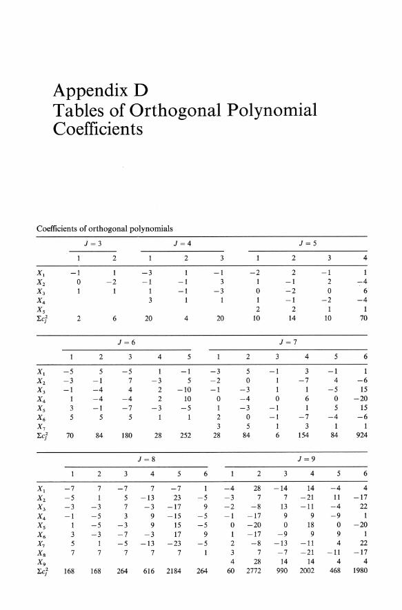
Appendix D Tables of Orthogonal Polynomial Coefficien ts
Coefficients of orthogonal polynomials
J=3 J=4 J=5
2 2 3 2
Xl -1 1 -3 -1 -2 2 X2 0 -2 -1 -1 3 -1 X3 1 -1 -3 0 -2 X4 3 1 -1 Xs 2 2 ~cJ 2 6 20 4 20 10 14
J=6 J=7
2 3 4 5 2 3 4
Xl -5 5 -5 -1 -3 5 -1 3 X2 -3 -1 7 -3 5 -2 0 -7 X3 -1 -4 4 2 -10 -1 -3 1 X4 1 -4 -4 2 10 0 -4 0 6 Xs 3 -1 -7 -3 -5 1 -3 -1 1 X6 5 5 5 1 2 0 -1 -7 X7 3 5 3 ~cJ 70 84 180 28 252 28 84 6 154
J=8 J=9
2 3 4 5 6 2 3 4
Xl -7 7 -7 7 -7 -4 28 -14 14 X2 -5 1 5 -13 23 -5 -3 7 7 -21 X3 -3 -3 7 -3 -17 9 -2 -8 13 -11 X4 -1 -5 3 9 -15 -5 -1 -17 9 9 Xs 1 -5 -3 9 15 -5 0 -20 0 18 X6 3 -3 -7 -3 17 9 17 -9 9 X7 5 1 -5 -13 -23 -5 2 -8 -13 -11 Xs 7 7 7 7 7 3 7 -7 -21 X9 4 28 14 14 ~cJ 168 168 264 616 2184 264 60 2772 990 2002
3 4
-1 1 2 -4 0 6
-2 -4 1
10 70
5 6
-1 4 -6
-5 15 0 -20 5 15
-4 -6 1 1
84 924
5 6
-4 4 11 -17
-4 22 -9 1
0 -20 9 1 4 22
-11 -17 4 4
468 1980

-9 -7 -5 -3 -1
1 3 5 7 9
330
J = 10
2 3 4 5 6
6 -42 18 -6 3 2 14 -22 14-11
-1 35 -17 -1 10 -3 31 3 -11 6 -4 12 18 -6 -8 -4 -12 18 6 -8 -3 -31 3 11 6 -1 -35 -17 1 10
2 -14 -22 -14 -11 6 42 18 6 3
132 8580 2860 780 660
J = 12
2 3 4 5 6
-11 55 -33 33 -33 11 -9 .25 -7 -5 -17 -3 -29 -1 -35
1 -35 3 -29 5 -17 7 9 25
11 55
572 12012
2
3 21 25 19 7
-7 -19 -25 -21 -3 33
5148
-27 57 -31 -33 21 11 -13 -29 25
12 -44 4 28 -20 -20 28 20 -20 12 44 4
-13 29 25 -33 -21 11 -27 -57 -31
33 33 11
8008 15912 4488
J = 14
3 4 5 6
XI -13 13 -143 143 -143 143 X 2 -11 X3 -9 X 4 -7 Xs -5 X6 -3 X 7 -1 Xs 1 X9 3 X IO 5 XII 7 X 12 9 X I3 11 XI4 13 XIS LeJ 910
7 -11 -77 187 -319 2 66 132 132 -11
-2 98 -92 -28 227 -5 95 -13 -139 185 -7 67 63 -145 -25 -8 -8 -7 -5 -2
2 7
13
24 108 -60 -200 -24 108 60 -200 -67 63 145 -25 -95 -13 139 185 -98 -92 28 227 -66 -132 -132 -11
11 -77 -187 -319 143 143 143 143
728 97240 136136 235144 497420
J = 11
2 3 4
-5 15 -30 6 -6 -4 6 6
-3 -1 22 -6 -2 -6 23 -1 -1 -9 14 4
6 4
o -10 0 1 -9 -14 2 -6 -23 -1 3 -1 -22 -6 4 6 -6 -6 5 15 30 6
286 110 858 4290
2
-6 22 -5 11 -4 2 -3 -5 -2 -10 -1 -13
o -14 -13
2 -10 3 -5 4 2 5 11 6 22
182 2002
2
J = 13
3 4
-11 99 o -66 6 -96 8 -54 7 11 4 64 o 84
-4 64 -7 11 -8 -54 -6 -96
o -66 11 99
572 68068
J = 15
3 4
5 6
-3 15 6 -48
29 -4 36 -4 -12
o -40 4 -12 4 36
-1 29 -6 -48
3 15 156 11220
5 6
-22 22 33 -55 18 8
-11 43 -26 22 -20 -20
o -40 20 -20 26 22 11 43
-18 8 -33 -55
22 22 6188 14212
5 6
-7 91 -91 1001 -1001 143 -6 52 -13 -429 1144 -286 -5 19 35 -869 979 -55 -4 -8 58 -704 44 176 -3 -29 61 -249 -751 197 -2 -44 49 251 -1000 50 -1 -53 27 621
o -56 0 756 -53 -27 621
2 -44 -49 251 3 -29 -61 -249 4 -8 -58 -704 5 19 -35 -869 6 52 13 -429 7 91 91 1001
-675 -125 o -200
675 -125 1000 50 751 197
-44 176 -979 -55
-1144 -286 1001 143
280 37128 39780 6446460 10581480 426360
Source: STATISTICS, 3je, by William L. Hays. Copyright © 1981 by CBS College Publishing. Reprinted by permission of Holt, Rinehart & Winston, Inc.
429

Problems
PROBLEMS FOR CHAPTER 2
1. Correlate the following pair of variables, X and Y. If possible, perform the analysis both by hand (or using a hand calculator) and with a computer package such as SAS or SPSSX. Also report the simple descriptive statistics (mean and standard deviation) of X and Y. Also, compute the covariance of X and Y.
x y
59 16 67 28 63 21 56 15 61 20 66 28 58 18 63 27 55 15 58 14 58 18 53 18 52 10 69 29 64 26 60 16 67 24 57 19 57 13 55 17
(Answer)
r = .88, X = 59.5, sx = 4.9, Y = 19.6, Sy = 5.6. The covariance is 24.15.
2. Repeat the analysis using the following data.

Problems 431
X Y
27 6 36 6 32 3 29 5 32 5 31 3 32 3 31 5 32 4 31 5 34 5 27 4 29 5 30 4 28 6 35 5 30 5 37 6 27 5 37 4
(Answer) r = .0, X = 31.35, sx = 3.17, Y = 4.70, Sy = .98. The covariance is .0.
3. Repeat the analysis using the following data.
X Y
48 -11 61 -18 56 -17 54 -15 45 -8 49 -12 53 -14 50 -11 52 -15 56 -15 58 -16 61 -19 56 -16 55 -17 63 -23 53 -16 51 -13 54 -14 46 -10 54 -15
(Answer) r = -.95, X = 53.8, Sx = 4.8, Y = -14.8, Sy = 3.4. The covariance is 15.61.
432 Problems
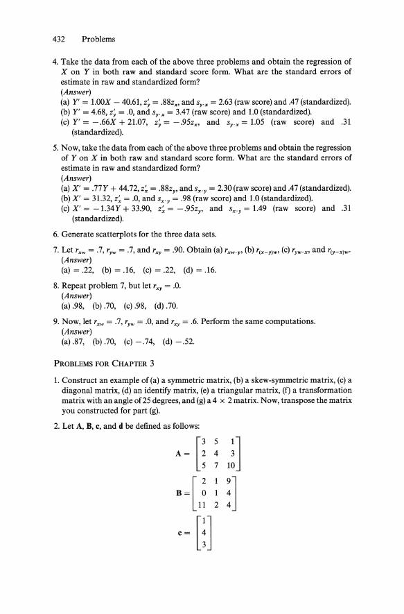
4. Take the data from each of the above three problems and obtain the regression of X on Y in both raw and standard score form. What are the standard errors of estimate in raw and standardized form? (Answer) (a) Y' = l.OOX - 40.61, z~ = .88zx, and Sy.x = 2.63 (raw score) and .47 (standardized). (b) Y' = 4.68, z~ = .0, and Sy.x = 3.47 (raw score) and 1.0 (standardized). (c) Y' = -.66X + 21.07, z~ = -.95zx , and Sy-x = 1.05 (raw score) and .31
(standardized).
5. Now, take the data from each of the above three problems and obtain the regression of Y on X in both raw and standard score form. What are the standard errors of estimate in raw and standardized form? (Answer) (a) X' = .77Y + 44.72, z~ = .88zy, and sx.y = 2.30 (raw score) and.47 (standardized). (b) X' = 31.32, z~ = .0, and sx.y = .98 (raw score) and 1.0 (standardized). (c) X' = -1.34 Y + 33.90, z~ = - .95zy, and sx.y = 1.49 (raw score) and .31
(standardized).
6. Generate scatterplots for the three data sets.
7. Let rxw = .7, ryw = .7, and rxy = .90. Obtain (a) rxw .y, (b) r(x-ylw, (c) ryw'x, and r(y-xlw' (Answer) (a) = .22, (b) = .16, (c) = .22, (d) = .16.
8. Repeat problem 7, but let rxy = .0. (Answer) (a) .98, (b) .70, (c) .98, (d) .70.
9. Now, let rxw = .7, ryW = .0, and rxy = .6. Perform the same computations. (Answer) (a) .87, (b) .70, (c) -.74, (d) -.52.
PROBLEMS FOR CHAPTER 3
1. Construct an example of (a) a symmetric matrix, (b) a skew-symmetric matrix, (c) a diagonal matrix, (d) an identify matrix, (e) a triangular matrix, (f) a transformation matrix with an angle of25 degrees, and (g) a 4 x 2 matrix. Now, transpose the matrix you constructed for part (g).
2. Let A, D, c, and d be defined as follows:
A~ U ~ In D = [ ~ :]
11 2 4
,~ m
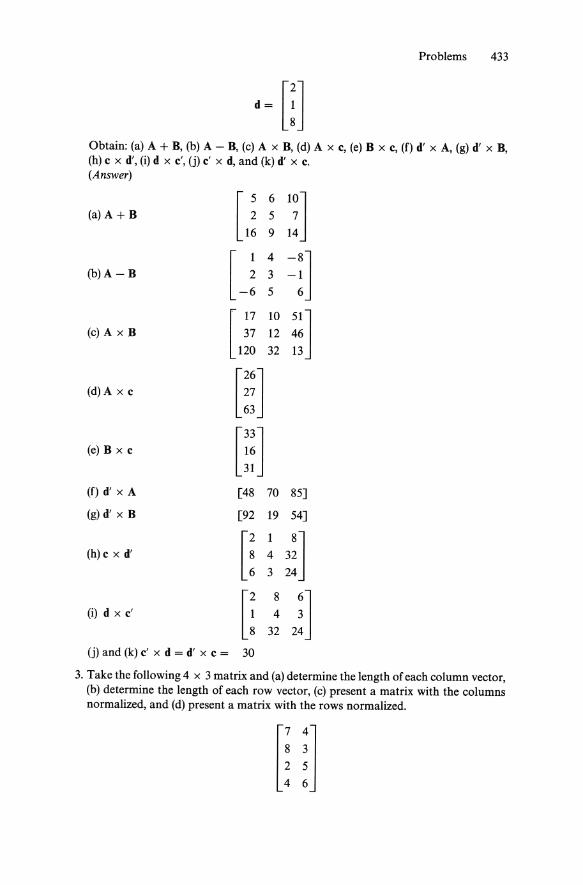
Problems 433
d~ m Obtain: (a) A + B, (b) A - B, (c) A x B, (d) A x c, (e) B x c, (f) d' x A, (g) d' x B, (h) c x d', (i) d xc', (j) c' x d, and (k) d' x c. (Answer)
(a) A + B
(b) A - B
(c) A x B
(d) A x c
(e) B x c
(f) d' x A
(g)d'xB
(h) c x d'
(i) d x c'
u ~ :!] [ ~ ~ =~]
-6 5 6
[ 17 10 51] 37 12 46
120 32 13
m] m] [48 70 85]
[92 19 54]
[: ; ~;] [: 3~ 2!]
(j) and (k) c' x d = d' x c = 30
3. Take the following 4 x 3 matrix and (a) determine the length of each column vector, (b) determine the length of each row vector, (c) present a matrix with the columns normalized, and (d) present a matrix with the rows normalized.
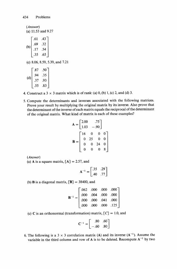
434 Problems
(Answer) (a) 11.53 and 9.27
l.61 A3j .69 .32
(b) .17 .54
.35 .65
(c) 8.06, 8.59, 5.39, and 7.21
l.87 .50j (d) .94 .35
.37 .93
.55 .83
4. Construct a 3 x 3 matrix which is of rank: (a) 0, (b) 1, (c) 2, and (d) 3.
5. Compute the determinants and inverses associated with the following matrices. Prove your result by multiplying the original matrix by its inverse. Also prove that the determinant ofthe inverse of each matrix equals the reciprocal of the determinant of the original matrix. What kind of matrix is each of these examples?
A = [2.00 .75J 1.03 -.90
B{~ 2~ ~ ~j (Answer) (a) A is a square matrix, [A] = 2.57, and
A-I = [.35 .29J AO .77
(b) B is a diagonal matrix, [B] = 38400, and
l.062 .000
B-1 = .000 .004 .000 .000
.000 .000
.000 .000j
.000 .000
.041 .000
.000 .125
(c) C is an orthonormal (transformation) matrix, [C] = 1.0, and
C-I = [ .80 .60J -.60 .80
6. The following is a 3 x 3 correlation matrix (A) and its inverse (A -I). Assume the variable in the third column and row of A is to be deleted. Recompute A -I by two

Problems 435
different methods. Prove your result by showing that the product of the reduced A and A -1 is an identity matrix.
l 10
0.6 0.3 -OIJ 0.6 1.0 0.2 0.7 A=
0.3 0.2 1.0 -0.3 -0.1 0.7 -0.3 1.0
l-68.84 116.05 -31.86
-9767l A- 1 = 116.05 -192.56 52.33 162.09
-31.86 52.33 -13.02 -43.72 -97.67 162.09 -43.72 -135.35
(Answer)
[ 1.65 -.93 -.31]
A-1 = -.93 1.56 -.03
-.31 -.03 1.10
7. Compute a correlation matrix from the following matrix of z-scores:
0.8088 -0.8967 0.9871 0.8879 -0.3408 -0.7828
-0.5941 -0.0665 1.2375 0.4133 -0.4817 0.6468
1.0606 0.8712 -0.6670
1.4429 1.5968 -1.9072
0.2165 1.1355 0.1263 -1.0482 -1.4922 0.4522
0.8358 0.9617 -1.0148 -1.7119 -1.1803 -0.2440
0.0748 -0.6570 -0.2731
-0.7794 -0.5892 0.3897 1.0548 -0.4482 2.1740 0.1176 -0.3414 1.5964
-1.1264 -0.0334 0.6755 1.5174 0.9932 -1.8991
-0.3155 0.1063 -0.4444 -1.7599 -0.4675 0.5675 -1.1370 0.3830 -0.9212
1.0077 0.1676 -0.1122
0.3224 -0.4186 -0.2139 -0.1206 1.0681 -0.5853
0.9490 2.6040 -1.0364
-0.9333 -1.4509 0.6549 -1.1709 -1.0085 0.5270

436 Problems
(Answer)
[ 1.000
0.557
-0.346
.557
1.000
-0.614
-0.346] -0.614
1.000
8. Verify Eq. (3-6) by using the following data. Apply the equation to both the sum and the difference. Also verify that the mean of the sum is the sum of the means and the mean of the difference is the difference of the means (see the section entitled the mean of a linear combination):
x y
26 53 8 43 11 38 7 20 -7 29 1 36 6 30 -2 35 8 42 3
(Answer) X = 35.2, Sx = 9.51, Y = 3.6, Sy = 5.46, and rxy = .797. Therefore, the mean of the sum is 38.8, the standard deviation of the sum is 14.25, the mean of the difference is 31.6, and the standard deviation of the difference is 6.11.
9. Compute the eigenvalues and normalized eigenvectors of symmetric matrix A and asymmetric matrix B. Note that the sum of the cross products of the eigenvector elements of A is zero, but the sum of the cross products of the eigenvector elements of B is not zero.
(Answer)
A = C! l~J B = [1~ ~~J
The eigenvalues of both matrices and 17.217 and 7.783. However, the eigenvectors of A are (.87, .48) and (-.87, .48), whereas the eigenvectors of Bare (.41, .91) and ( - .13, .99).
PROBLEMS FOR CHAPTER 4
1. Using the following data in which X and Yare the predictors and C is the criterion, compute R, R2, the standardized and raw score regression equations, and the F ratio associated with a test of the null hypothesis that R = O. Perform the analysis both by hand, using Eqs. (4-4) to (4-6) and through an SPSSX, SAS, BMDP, or similar package. Also, use the data to verify Eqs. (4-7) to (4-9).

Problems 437
C X Y
12 98 23 9 92 26
14 111 36 11 118 25 8 98 28
15 87 39 11 101 20 8 108 27 9 100 24 7 86 19
10 81 32 15 101 34 14 111 34 10 112 24 16 109 39 9 89 34
17 112 39 13 91 31 6 88 21 9 100 25
11 117 26 14 98 35 14 110 34 11 88 31 14 111 37 12 110 21 10 94 31 9 87 30
11 114 27 16 103 38 14 109 37 14 106 32 9 90 25
10 98 24 12 100 27 15 113 34 16 101 39 9 124 23
10 92 34 8 96 28
10 94 23 10 97 29 16 110 42 14 111 32 12 108 24 10 94 34 9 87 28
11 98 25 12 98 33 10 94 21
(Answer)
R = .82, R2 = .6724, z; = .355zx + .700zy, C' = .096X + .318Y - 7.630, F(2,47) = 48.04, p < .0001.

438 Problems
2. Let R = a 2 x 2 correlation matrix with r"y as its off-diagonal element and v be the vector containing the respective correlations of X and Y with C, using results obtained from problem 1. Obtain R-1 and compute R2 and the standardized regression equation from these data.
3. Perform the same analyses upon the following data. What role does Y play in the analysis?
c X Y
19 98 71 12 86 64 15 93 62 16 96 61 10 101 73 16 88 68 19 82 58 9 84 57
14 91 65 14 62 49 12 69 56 19 76 53 15 90 60 15 100 67 17 102 69 8 108 82
19 104 70 18 94 71 10 74 57 12 90 64
(Answer) R = .38,R2 = .1408,z; = .859z" - .754zy, C' = .298X - .218Y + 13.852, F(2,47) = 3.85, p < .03. Y is a suppressor variable, as its correlation with C is effectively zero (.01) yet its beta weight is substantial (-.753) due to its correlation with X.
4. In the following problem, let X, Y, and Z be predictors of C. Input the data to a compute package and analyze the results, providing the same results you obtained from the data of problem 1.
c X Y Z
17 5 15 8 17 2 16 5 19 3 15 7 18 5 15 10 25 5 23 11 14 3 21 8 14 3 20 8 12 6 17 5 13 4 14 9 13 3 17 8 8 5 19 3
20 7 17 7

Problems 439
C X Y Z
15 2 22 8 16 4 16 7 11 3 12 8 14 4 22 12 12 4 15 9 12 4 19 9 19 7 19 7 12 3 14 4 8 2 12 8
13 6 8 8 18 5 13 9 13 3 17 9 20 6 17 8 18 4 19 8 19 4 17 8 14 6 13 7 16 5 20 6 12 3 19 8 22 4 21 8 19 3 20 5 14 5 14 10 17 4 21 8 17 3 13 4 11 3 14 7 11 4 13 4 13 4 12 3 20 3 18 10 19 7 21 7 12 7 13 3 18 6 19 7 13 3 19 3 17 6 20 6 20 4 20 8 21 4 16 5 18 4 18 6 11 4 19 5 21 1 8 8 10 5 9 6 10 6 6 9 17 5 16 7 13 2 21 8 8 3 16 5
15 4 16 8 11 6 18 9 14 4 22 4 17 6 11 11 17 3 18 7 21 3 13 6
(Answer)
R = .34, R2 = .1197, z; = .104zx + .256zy + .199z., C' = .285X + .261 Y + 371Z, F(3,56) = 2.54, ns.

440 Problems
5. Perform the same analysis upon the following data that was performed in answer to question 4.
C X Y Z
11 6 20 8 17 4 14 9 14 5 23 6 17 4 13 4 15 5 18 8 16 6 12 6 9 3 17 7
16 5 12 4 7 0 16 6 9 4 21 4
22 5 16 7 18 4 12 9 11 4 13 9 23 8 23 10 14 4 20 9 11 2 12 3 11 4 9 10 15 5 16 9 17 6 19 7 5 4 15 7
21 4 22 8 15 0 12 6 12 5 12 7 15 7 12 6 19 5 19 9 20 4 3 9 14 6 20 6 14 5 14 5 13 3 15 8 18 4 19 11 26 5 25 6 14 3 14 5 7 3 15 6
10 3 12 8 10 2 13 8 23 5 21 10 12 5 16 9 12 5 14 9 9 3 15 7
24 4 19 8 13 4 19 10 11 2 17 8 9 3 10 8
11 7 14 9 17 6 14 8 14 6 17 7 19 4 23 7 13 4 18 6 17 7 13 8
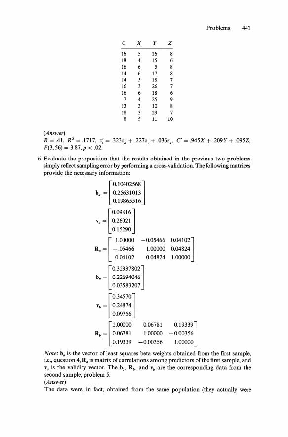
Problems 441
C X Y Z
16 5 16 8 18 4 15 6 16 6 5 8 14 6 17 8 14 5 18 7 16 3 26 7 16 6 18 6 7 4 25 9
13 3 10 8 18 3 29 7 8 5 11 10
(Answer) R = .41, R2 = .1717, z; = .323zx + .227zy + .036z., C' = .945X + .209Y + .095Z, F(3,56) = 3.87, p < .02.
6. Evaluate the proposition that the results obtained in the previous two problems simply reflect sampling error by performing a cross-validation. The following matrices provide the necessary information:
[0.10402568]
ba = 0.25631013
0.19865516
Va = [~:~:~~~] 0.15290
[ 1.00000
Ra = -.05466
0.04102
-0.05466
1.00000
[0.32337802]
bb = 0.22694046
0.03583207
Vb = [~:~::~~] 0.09756
0.04824
[1.00000 0.06781
Rb = 0.06781 1.00000
0.19339 -0.00356
0.04102] 0.04824
1.00000
0.19339] -0.00356
1.00000
Note: ba is the vector ofleast squares beta weights obtained from the first sample, i.e., question 4, Ra is matrix of correlations among predictors ofthe first sample, and Va is the validity vector. The bb' Rb, and Vb are the corresponding data from the second sample, problem 5. (Answer) The data were, in fact, obtained from the same population (they actually were

442 Problems
generated with different random number seeds). The value of r2 obtain by applying hb to Ra is .0642, and the respective F -ratios are 1.76 and 2.04 (dJ = 2 and 56). Neither is significant.
7. How highly correlated are the predicted scores using ba and hb (a) within Ra and (b) within Rb? (Answer) (a) .73 and (b) .80 (note that the "It don't make no nevermind" principle is less applicable here than in many other situations because the correlations among the variables are relatively small).
8. Apply unit weights to the two correlation matrices. Determine r2 and test the significance of the difference from the least squares R 2 values in the two samples. (Answer) The two values ofr2 are .1072 and .1362. The associated F ratios are < 1.0 and 1.13 (dJ = 2 and 56). Note that unit weighting actually provided more stable results across samples than the least squares weights (although the difference was not significant).
9. The following matrices are the inverse of Ra and the inverse of the corresponding R* matrix (the 4 x 4 matrix with the validities added). Use these data, as well as the preceding data from Ra to perform an "all subsets regression," i.e., compute values of R2 associated with all combinations of the three predictors. Perform the computations using the matrix equations in the book. Then compare your results to the output of computer package performing the same analysis, e.g., SAS PROC RSQUARE. (Answer)
Predictors R2
X 0.0096 Y 0.0463 Z 0.0677 X,Y 0.0543 X,Z 0.0803 Y,Z 0.1089 X, Y,Z 0.1197
PROBLEMS FOR CHAPTER 5
1. Assume that subjects are assigned to one of four groups in a learning task. Group A is a control Group, and Groups B, C, and D represent three different types of instructions. The data (percentage of words correctly recalled) are as follows. Perform an ANOV A: (a) by hand using the conventional (partitioning of sums of squares) method, (b) using a relevant computer package, (c) using dummy codes, (d) using effect codes, and (e) using orthogonal codes. Use Group A as the target Group and let the contrasts be: (1) Groups A and C versus Groups Band D, (2) Groups A and B versus Groups C and D, and (3) Groups A and D versus Groups Band C. Present the regression equations derived from the dummy, effect, and orthogonal coding. Indicate which comparisons are significant.
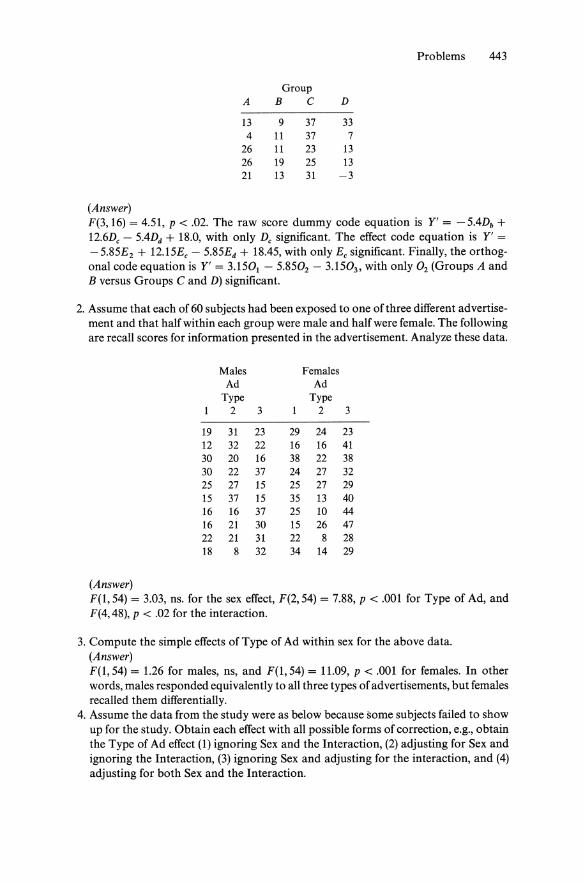
Problems 443
Group A B C D
13 9 37 33 4 11 37 7
26 11 23 13 26 19 25 13 21 13 31 -3
(Answer)
F(3, 16) = 4.51, p < .02. The raw score dummy code equation is Y' = - 5.4Db + 12.6Dc - 5.4Dd + 18.0, with only Dc significant. The effect code equation is Y' = - 5.85E2 + 12.15Ec - 5.85Ed + 18.45, with only Ec significant. Finally, the orthogonal code equation is Y' = 3.1501 - 5.8502 - 3.1503 , with only O2 (Groups A and B versus Groups C and D) significant.
2. Assume that each of 60 subjects had been exposed to one ofthree different advertisement and that half within each group were male and half were female. The following are recall scores for information presented in the advertisement. Analyze these data.
Males Females Ad Ad
Type Type 2 3 2 3
19 31 23 29 24 23 12 32 22 16 16 41 30 20 16 38 22 38 30 22 37 24 27 32 25 27 15 25 27 29 15 37 15 35 13 40 16 16 37 25 10 44 16 21 30 15 26 47 22 21 31 22 8 28 18 8 32 34 14 29
(Answer)
F(I,54) = 3.03, ns. for the sex effect, F(2,54) = 7.88, p < .001 for Type of Ad, and F( 4,48), p < .02 for the interaction.
3. Compute the simple effects of Type of Ad within sex for the above data. (Answer)
F(I,54) = 1.26 for males, ns, and F(I,54) = 11.09, p < .001 for females. In other words, males responded equivalently to all three types of advertisements, but females recalled them differentially.
4. Assume the data from the study were as below because some subjects failed to show up for the study. Obtain each effect with all possible forms of correction, e.g., obtain the Type of Ad effect (1) ignoring Sex and the Interaction, (2) adjusting for Sex and ignoring the Interaction, (3) ignoring Sex and adjusting for the interaction, and (4) adjusting for both Sex and the Interaction.

444 Problems
Males Females Ad Ad
Type Type 2 3 2 3
19 31 23 29 24 23 12 32 22 16 16 41 30 20 16 38 22 38 30 22 37 24 27 32 25 27 15 25 27 29 15 37 15 35 13 40 16 16 37 25 10 44 16 21 30 15 26 47 22 21 31 22 8 28 18 8 32 34 14 29
(Answer)
Effect Adjusting for F p
Sex .31 ns Sex Type .41 ns Sex Interaction * Sex Type, Interaction * Type 1.98 ns Type Sex 2.19 ns Type Interaction * Type Sex, Interaction * Interaction 2.22 ns Interaction Sex 2.77 .04 Interaction Type 2.19 ns Interaction Sex, Type 3.36 .04
Note: Effects designated by an asterisk (*) were not computable due to the correlation between the interaction and the main effects.
5. Assume that you ran a study like that in problem number 1, and obtained a covariate measure (X) for each subject, as well as the dependent variable (Y). Analyze the results, and be sure to test for homogeneity of regression.
Group A B C D
Y X Y X Y X Y X
13 7 28 32 24 12 16 7 26 32 14 12 15 13 26 23 21 17 22 31 13 -5 10 14 9 6 9 6 41 34 10 1
17 15 15 2 34 28 6 10
(Answer) F(I, 12) = 44.76, p < .0001 for the Covariate, F(3, 12) = 3.14, ns, for the Groups x Covariate interaction, and F(3, 12) < 1, ns, for the Groups effect. Thus, the only determinant of Y is the covariate, X.

Problems 445
6. Now suppose a study of similar design yielded the following results. Analyze the data.
Group A B C D
Y X Y X Y X Y X
21 16 24 17 25 16 28 16 22 17 23 16 24 17 29 15 21 16 23 17 24 15 28 16 21 16 23 16 26 16 28 16 21 16 23 15 25 16 28 17
(Answer) F(I, 12) = 5.74, ns, for the Covariate, F(3, 12) = 140.06, p < .0001 for the Group x Covariate interaction, and F(3, 12) = 2.80, ns, for the Group effect. The significant interaction illustrates differences in slope among groups (X and Yare positively related in-Groups A and B, unrelated in Group C, and negatively related in Group D).
7. Analyze the following data in two different ways: (1) as a repeated measure design with each of seven subjects tested under five conditions, and (2) as an independent groups design with subjects randomly assigned to each group.
Treatment A B C D E
102 102 109 108 115 110 117 126 117 127 91 87 87 100 96 99 101 98 97 97 96 100 97 96 107
110 113 109 126 119 97 101 103 109 107
(Answer) Viewed as a repeated design experiment, F(4, 24) = 4.57, p < .01. This is because the error term is Treatment x Subjects, whose mean square is 18.90 with 24 df Viewed as an independent groups experiment, F(4, 28) < 1, ns. This is because the error term is subjects within groups whose mean square is 109.91 with 30 df Though simulated, the outcome is typical of most situations.
PROBLEMS FOR CHAPTER 6
1. The following hypothetical data are derived from 50 subjects who took 10 tests of cognitive abilities, each scaled to a mean of 100 and a standard deviation of 15. The tests are designated Xl to X 10. Explore their factor structure by means of a component analysis. (Note that in actual practice, the number of cases would be far too small; this problem, as well as the two that follow are included to demonstrate certain important raw data structures.)
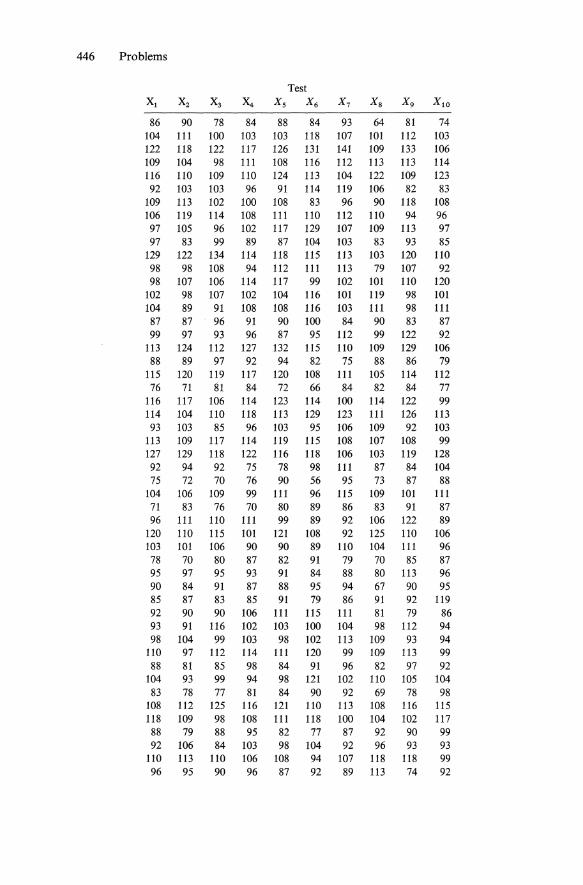
446 Problems
Test Xl X2 X3 X4 Xs X6 X 7
86 90 78 84 88 84 93 64 81 74 104 111 100 103 103 118 107 101 112 103 122 118 122 117 126 131 141 109 133 106 109 104 98 111 108 116 112 113 113 114 116 110 109 110 124 113 104 122 109 123 92 103 103 96 91 114 119 106 82 83
109 113 102 100 108 83 96 90 118 108 106 119 114 108 111 110 112 110 94 96 97 105 96 102 117 129 107 109 113 97 n ~ ~ ~ ~ 104 100 83 93 85
129 122 134 114 118 115 113 103 120 110 98 98 108 94 112 111 113 79 107 92 98 107 106 114 117 99 102 101 110 120
102 98 107 102 104 116 101 119 98 101 104 89 91 108 108 116 103 111 98 III 87 87 96 91 90 100 84 90 83 87 99 97 93 96 87 95 112 99 122 92
113 124 112 127 132 115 110 109 129 106 88 89 97 92 94 82 75 88 86 79
115 120 119 117 120 108 111 105 114 112 76 71 81 84 72 66 84 82 84 77
116 117 106 114 123 114 100 114 122 99 114 104 110 118 113 129 123 III 126 113 93 103 85 96 103 95 106 109 92 103
113 109 117 114 119 115 108 107 108 99 127 129 118 122 116 118 106 103 119 128 92 94 92 75 78 98 111 87 84 104 75 72 70 76 90 56 95 73 87 88
104 106 109 99 III 96 115 109 101 III 71 83 76 70 80 89 86 83 91 87 96 111 110 111 99 89 92 106 122 89
120 110 115 101 121 108 92 125 110 106 103 101 106 90 90 89 110 104 III 96 78 70 80 87 82 91 79 70 85 87 95 97 95 93 91 84 88 80 113 96 90 84 91 87 88 95 94 67 90 95 85 87 83 85 91 79 86 91 92 119 92 90 90 106 111 115 111 81 79 86 93 91 116 102 103 100 104 98 112 94 98 104 99 103 98 102 113 109 93 94
110 97 112 114 111 120 99 109 113 99 88 81 85 98 84 91 96 82 97 92
104 93 99 94 98 121 102 110 105 104 83 78 77 81 84 90 92 69 78 98
108 112 125 116 121 110 113 108 116 115 118 109 98 108 111 118 100 104 102 117 88 79 88 95 82 77 87 92 90 99 92 1~ ~ 100 ~ 104 92 96 93 93
110 113 110 106 108 94 107 118 118 99 96 95 90 96 87 92 89 113 74 92

Problems 447
(Answer) The first four eigenvalues are 6.87, .74, .56, and .50. By virtually any definition (number of eigenvalues> 1, scree, etc.), the data can be well represented by a single factor. The pattern for the first principal component, which accounts for .687 of the total variance, and the associated h2 values is as follows. Note that tests Xl to Xs load more heavily upon the factor than do tests X6 to X IO .
Variable Component h2
Xl .939 .882 X2 .899 .808 X3 .872 .761 X4 .898 .806 Xs .905 .819 X6 .772 .596 X7 .694 .482 Xs .777 .603 Xg .801 .642 XIO .689 .474
Variables Xl to X 5 were actually generated by equations of the form Y = .90F + .43e, and variables X6 to XIO were generated by equations of the form Y = .70F + .71e. F and e are random normal deviates (0, 1). F is common to all 10 equations and e is unique to each. Since .902 + .432 = .702 + .712 = 1 and e and F are independent, the variance of Y is 1.0.
2. Now, perform the same analysis upon the following data.
Test Xl X2 X3 X4 Xs X6 X7 Xs Xg XIO Xli Xl2
123 101 111 119 107 116 64 80 74 85 79 87 90 109 97 91 100 92 101 98 91 94 89 98
121 147 117 137 130 123 102 122 117 128 125 125 120 105 92 95 97 117 106 98 114 105 114 109 102 89 80 112 116 104 64 65 84 87 91 79 89 103 96 125 116 119 88 107 100 91 94 96 84 87 105 89 101 88 98 121 126 105 107 110
103 78 107 89 86 103 100 82 91 85 104 98 97 105 111 113 104 119 90 102 86 88 100 84
114 77 108 95 112 91 108 106 119 121 106 109 118 104 105 100 114 106 99 109 95 106 92 94 76 79 111 109 114 102 110 98 111 97 100 101
103 112 94 101 95 98 108 119 116 113 116 106 119 143 111 133 106 122 85 107 115 98 94 94
81 90 92 101 94 97 105 99 110 111 106 126 95 92 98 91 94 88 89 86 76 86 80 91 69 89 87 86 80 92 120 122 105 116 126 114
126 101 123 104 88 98 95 87 108 99 91 101 90 107 74 95 106 95 106 108 94 102 106 100
111 119 114 108 107 107 85 111 103 102 89 94 88 85 102 110 95 100 93 89 64 73 91 100
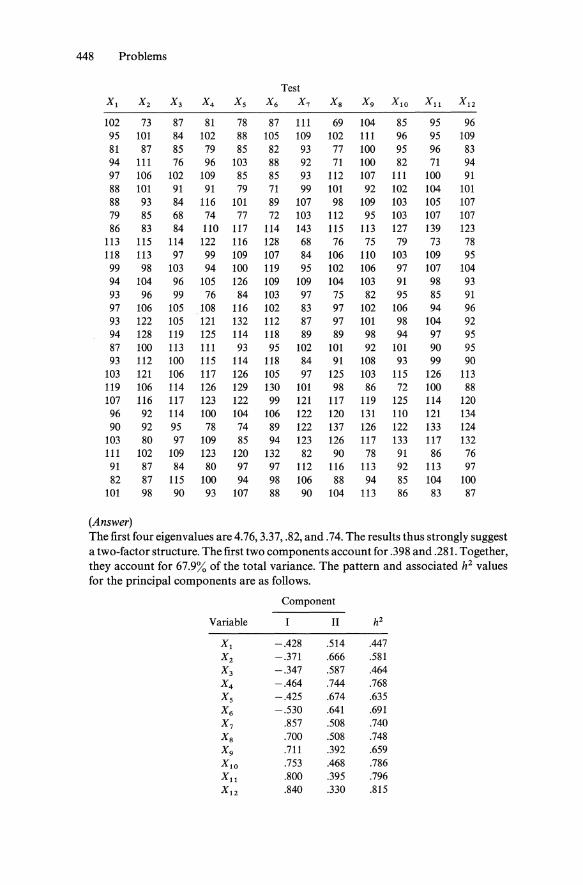
448 Problems
Test Xl X2 X3 X4 Xs X6 X7 Xs Xg X ID Xll Xl2
102 73 87 81 78 87 111 69 104 85 95 96 95 101 84 102 88 105 109 102 111 96 95 109 81 87 85 79 85 82 93 77 100 95 96 83 94 111 76 96 103 88 92 71 100 82 71 94 97 106 102 109 85 85 93 112 107 111 100 91 88 101 91 91 79 71 99 101 92 102 104 101 88 93 84 116 101 89 107 98 109 103 105 107 79 85 68 74 77 72 103 112 95 103 107 107 86 83 84 110 117 114 143 115 113 127 139 123
113 115 114 122 116 128 68 76 75 79 73 78 118 113 97 99 109 107 84 106 110 103 109 95 99 98 103 94 100 119 95 102 106 97 107 104 94 104 96 105 126 109 109 104 103 91 98 93 93 96 99 76 84 103 97 75 82 95 85 91 97 106 105 108 116 102 83 97 102 106 94 96 93 122 105 121 132 112 87 97 101 98 104 92 94 128 119 125 114 118 89 89 98 94 97 95 87 100 113 111 93 95 102 101 92 101 90 95 93 112 100 115 114 118 84 91 108 93 99 90
103 121 106 117 126 105 97 125 103 115 126 113 119 106 114 126 129 130 101 98 86 72 100 88 107 116 117 123 122 99 121 117 119 125 114 120 96 92 114 100 104 106 122 120 131 110 121 134 90 92 95 78 74 89 122 137 126 122 133 124
103 80 97 109 85 94 123 126 117 133 117 132 111 102 109 123 120 132 82 90 78 91 86 76 91 87 84 80 97 97 112 116 113 92 113 97 82 87 115 100 94 98 106 88 94 85 104 100
101 98 90 93 107 88 90 104 113 86 83 87
(Answer) The first four eigenvalues are 4.76,3.37, .82, and .74. The results thus strongly suggest a two-factor structure. The first two components account for .398 and .281. Together, they account for 67.9% of the total variance. The pattern and associated h2 values for the principal components are as follows.
Component
Variable II h2
Xl -.428 .514 .447 X2 -.371 .666 .581 X3 -.347 .587 .464 X4 -.464 .744 .768 Xs -.425 .674 .635 X6 -.530 .641 .691 X7 .857 .508 .740 Xs .700 .508 .748 Xg .711 .392 .659 XlO .753 .468 .786 X1l .800 .395 .796 X12 .840 .330 .815

Problems 449
Note that the results consist of a unipolar and a bipolar factor. More commonly, the unipolar factor will be the first principal component than the second, in contrast to what was observed here. Variables Xl to X3 tend to have lower communalities than variables X 4 to X6 and variables X 7 to Xg tend to have lower communalities than variables Xg to X 12 • Most importantly, variables Xl to X6 tend to have higher loadings on Component II than Component I, but the reverse is true of variables X 7 to X 12 • The raw data suggest two relatively independent factors, which is actually how the data were generated. The outcome is not completely clear in the factor analysis because of the smaIl sample size, but see problem 5, where the results will be clearer. Variables Xl to X3 were defined by equations of the form Y = .63F, + .77e; variables X 4 to X6 were defined by equations of the form Y = .76F; + .65e; variables X 7 to Xg were defined by equations of the form Y = .76Fn + .65e, and; variables XlO to X12 were defined by equations of the form Y = .87Fn + .4ge.
3. Perform the same analysis upon the following raw data.
118 96 107 112 100 109 69 85 79 88 82 87 106 95 87 96 88 100 96 90 93 87
125 151 121 142 135 128 113 132 128 135 132 122 106 94 97 99 119 109 101 116 106 116 97 84 76 105 109 97 66 66 86 88 92 87 101 94 123 114 116 92 112 104 94 97 85 87 106 90 102 89 98 121 126 106 107
102 77 105 87 83 100 98 80 89 84 103 96 104 110 111 102 117 97 109 93 93 104
117 79 110 98 116 95 110 108 121 123 108 116 102 104 98 112 104 101 111 97 107 93 77 80 111 110 115 103 111 99 111 98 101
106 115 98 106 99 103 108 119 117 113 116 118 142 110 131 104 120 92 114 122 103 99 85 94 96 107 100 104 100 93 105 108 103 93 90 96 88 91 85 89 87 76 86 80 72 91 89 90 84 96 114 116 100 113 122
124 99 121 101 85 95 99 91 112 102 94 90 107 74 95 106 95 106 108 93 102 106
109 117 112 105 104 105 89 115 107 104 92 85 83 100 107 91 96 94 91 65 74 92
101 71 85 80 76 85 107 65 100 83 92 97 103 85 105 90 108 107 100 109 95 93 79 86 83 76 83 79 86 71 93 90 91 90 108 72 91 98 83 89 68 97 80 69 97 107 103 110 86 86 92 112 106 110 100 88 101 91 91 80 72 93 95 86 97 100 89 94 84 117 102 90 106 98 108 103 104 82 88 70 77 81 76 93 103 85 97 100 95 92 92 122 129 126 140 112 110 126 138
106 108 107 111 106 117 78 86 85 85 79 118 113 96 98 108 106 85 108 111 104 110 100 99 103 95 101 120 98 105 109 99 109
93 104 96 104 125 108 112 107 106 93 100
90 97
133 110 80 99
110 96 89
110 95
101 106 99
123 91
110 104 100 96
101 93
107 78 91 90 97
106 100 122 84 96
106 95
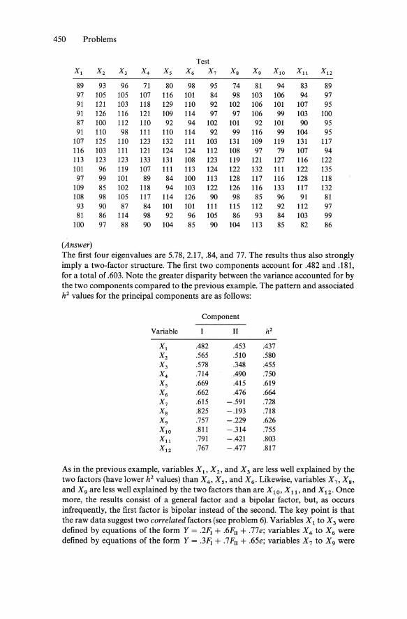
450 Problems
Test Xl X2 X3 X4 Xs X6 X7 Xs Xg XID XII Xl2
89 93 96 71 80 98 95 74 81 94 83 89 97 105 105 107 116 101 84 98 103 106 94 97 91 121 103 118 129 110 92 102 106 101 107 95 91 126 116 121 109 114 97 97 106 99 103 100 87 100 112 110 92 94 102 101 92 101 90 95 91 110 98 111 110 114 92 99 116 99 104 95
107 125 110 123 132 111 103 131 109 119 131 117 116 103 111 121 124 124 112 108 97 79 107 94 113 123 123 133 131 108 123 119 121 127 116 122 101 96 119 107 111 113 124 122 132 111 122 135 97 99 101 89 84 100 113 128 117 116 128 118
109 85 102 118 94 103 122 126 116 133 117 132 108 98 105 117 114 126 90 98 85 96 91 81 93 90 87 84 101 101 111 115 112 92 112 97 81 86 114 98 92 96 105 86 93 84 103 99
100 97 88 90 104 85 90 104 113 85 82 86
(Answer) The first four eigenvalues are 5.78, 2.17, .84, and 77. The results thus also strongly imply a two-factor structure. The first two components account for .482 and .181, for a total of .603. Note the greater disparity between the variance accounted for by the two components compared to the previous example. The pattern and associated hZ values for the principal components are as follows:
Component
Variable II h2
Xl .482 .453 .437 X2 .565 .510 .580 X3 .578 .348 .455 X4 .714 .490 .750 Xs .669 .415 .619 X6 .662 .476 .664 X7 .615 -.591 .728 Xs .825 -.193 .718 Xg .757 -.229 .626 XIO .811 -.314 .755 X ll .791 -.421 .803 X12 .767 -.477 .817
As in the previous example, variables Xl' Xz, and X3 are less well explained by the two factors (have lower hZ values) than X 4 , X s, and X 6 • Likewise, variables X 7 , X g ,
and X9 are less well explained by the two factors than are X10' Xu, and X1Z ' Once more, the results consist of a general factor and a bipolar factor, but, as occurs infrequently, the first factor is bipolar instead of the second. The key point is that the raw data suggest two correlated factors (see problem 6). Variables Xl to X3 were defined by equations of the form Y = .2F( + .6Fn + .77e; variables X 4 to X6 were defined by equations of the form Y = .3F( + .7Fn + .65e; variables X 7 to X9 were
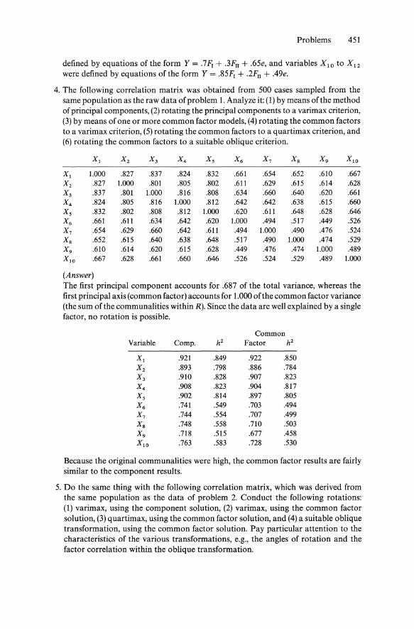
Problems 451
defined by equations of the form Y = .7FI + .3Fn + .65e, and variables X10 to X12
were defined by equations of the form Y = .85FJ + .2Fn + .4ge.
4. The following correlation matrix was obtained from 500 cases sampled from the same population as the raw data of problem 1. Analyze it: (1) by means ofthe method of principal components, (2) rotating the principal components to a varimax criterion, (3) by means of one or more common factor models, (4) rotating the common factors to a varimax criterion, (5) rotating the common factors to a quartimax criterion, and (6) rotating the common factors to a suitable oblique criterion.
Xl Xz X3 X4 Xs X6 X7 Xs Xg XIO
Xl 1.000 .827 .837 .824 .832 .661 .654 .652 .610 .667 Xz .827 1.000 .801 .805 .802 .611 .629 .615 .614 .628
X3 .837 .801 1.000 .816 .808 .634 .660 .640 .620 .661 X4 .824 .805 .816 1.000 .812 .642 .642 .638 .615 .660
Xs .832 .802 .808 .812 1.000 .620 .611 .648 .628 .646
X6 .661 .611 .634 .642 .620 1.000 .494 .517 .449 .526 X7 .654 .629 .660 .642 .611 .494 1.000 .490 .476 .524
Xa .652 .615 .640 .638 .648 .517 .490 1.000 .474 .529 Xg .610 .614 .620 .615 .628 .449 .476 .474 1.000 .489 XIO .667 .628 .661 .660 .646 .526 .524 .529 .489 1.000
(Answer) The first principal component accounts for .687 of the total variance, whereas the first principal axis (common factor) accounts for 1.000 of the common factor variance (the sum of the communalities within R). Since the data are well explained by a single factor, no rotation is possible.
Common Variable Compo hZ Factor h2
Xl .921 .849 .922 .850 X2 .893 .798 .886 .784
X3 .910 .828 .907 .823 X4 .908 .823 .904 .817
Xs .902 .814 .897 .805
X6 .741 .549 .703 .494 X7 .744 .554 .707 .499
Xs .748 .558 .710 .503 Xg .718 .515 .677 .458 XIO .763 .583 .728 .530
Because the original communalities were high, the common factor results are fairly similar to the component results.
5. Do the same thing with the following correlation matrix, which was derived from the same population as the data of problem 2. Conduct the following rotations: (1) varimax, using the component solution, (2) varimax, using the common factor solution, (3) quartimax, using the common factor solution, and (4) a suitable oblique transformation, using the common factor solution. Pay particular attention to the characteristics of the various transformations, e.g., the angles of rotation and the factor correlation within the oblique transformation.
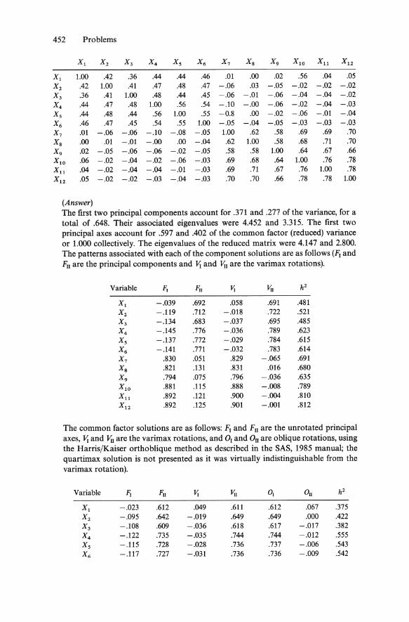
452 Problems
X, X2 X3 X4 Xs X6 X7 Xs Xg XlO X" X,2
X, 1.00 .42 .36 .44 .44 .46 .01 .00 .02 .56 .04 .05 X2 .42 1.00 .41 .47 .48 .47 -.06 .03 -.05 -.02 -.02 -.02 X3 .36 .41 1.00 .48 .44 .45 -.06 -.01 -.06 -.04 -.04 -.02 X4 .44 .47 .48 1.00 .56 .54 -.10 -.00 -.06 -.02 -.04 -.03 Xs .44 .48 .44 .56 1.00 .55 -0.8 .00 -.02 -.06 -.01 -.04 X6 .46 .47 .45 .54 .55 1.00 -.05 -.04 -.05 -.03 -.03 -.03 X7 .01 -.06 -.06 -.10 -.08 -.05 1.00 .62 .58 .69 .69 .70 Xs .00 .01 -.01 -.00 .00 -.04 .62 1.00 .58 .68 .71 .70 X9 .02 -.05 -.06 -.06 -.02 -.05 .58 .58 1.00 .64 .67 .66 XlO .06 -.02 -.04 -.02 -.06 -.03 .69 .68 .64 1.00 .76 .78
X" .04 -.02 -.04 -.04 -.01 -.03 .69 .71 .67 .76 1.00 .78 X12 .05 -.02 -.02 -.03 -.04 -.03 .70 .70 .66 .78 .78 1.00
(Answer) The first two principal components account for .371 and .277 of the variance, for a total of .648. Their associated eigenvalues were 4.452 and 3.315. The first two pdncipal axes account for .597 and .402 of the common factor (reduced) variance or 1.000 collectively. The eigenvalues of the reduced matrix were 4.147 and 2.800. The patterns associated with each ofthe component solutions are as follows (FJ and Fn are the principal components and l'l and l'll are the varimax rotations).
Variable F, FI, Vi Vi, h2
X, -.039 .692 .058 .691 .481 X2 -.119 .712 -.018 .722 .521 X3 -.134 .683 -.037 .695 .485 X4 -.145 .776 -.036 .789 .623 Xs -.137 .772 -.029 .784 .615 X6 -.141 .771 -.032 .783 .614 X7 .830 .051 .829 -.065 .691 Xs .821 .131 .831 .016 .680 Xg .794 .075 .796 -.036 .635 X,O .881 .115 .888 -.008 .789
X" .892 .121 .900 -.004 .810 X12 .892 .125 .901 -.001 .812
The common factor solutions are as follows: FI and Fn are the unrotated principal axes, l'l and Vn are the varimax rotations, and 01 and On are oblique rotations, using the Harris/Kaiser orthoblique method as described in the SAS, 1985 manual; the quartimax solution is not presented as it was virtually indistinguishable from the varimax rotation).
Variable FI Fn Vi Vi, 0, Ou h2
X, -.023 .612 .049 .611 .612 .067 .375 X2 -.095 .642 -.019 .649 .649 .000 .422 X3 -.108 .609 -.036 .618 .617 -.017 .382 X4 -.122 .735 -.035 .744 .744 -.012 .555 Xs -.115 .728 -.028 .736 .737 -.006 .543 X6 -.117 .727 -.031 .736 .736 -.009 .542
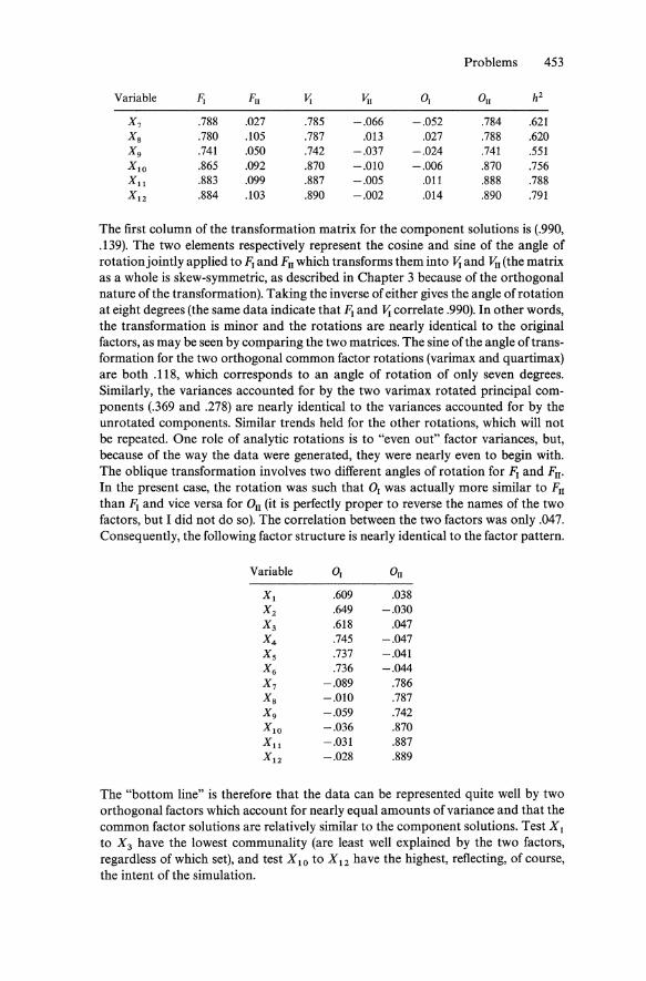
Problems 453
Variable FI FII Vi Vii 0 1 011 il2
X7 .788 .027 .785 -.066 -.052 .784 .621 Xs .780 .105 .787 .013 .027 .788 .620 X9 .741 .050 .742 -.037 -.024 .741 .551 X IO .865 .092 .870 -.010 -.006 .870 .756 Xu .883 .099 .887 -.005 .011 .888 .788 X l2 .884 .103 .890 -.002 .014 .890 .791
The first column of the transformation matrix for the component solutions is (.990, .139). The two elements respectively represent the cosine and sine of the angle of rotation jointly applied to fJ and FII which transforms them into J-j and VII (the matrix as a whole is skew-symmetric, as described in Chapter 3 because of the orthogonal nature of the transformation). Taking the inverse of either gives the angle of rotation at eight degrees (the same data indicate that FJ and J-j correlate .990). In other words, the transformation is minor and the rotations are nearly identical to the original factors, as may be seen by comparing the two matrices. The sine of the angle oftransformation for the two orthogonal common factor rotations (varimax and quartimax) are both .118, which corresponds to an angle of rotation of only seven degrees. Similarly, the variances accounted for by the two varimax rotated principal components (.369 and .278) are nearly identical to the variances accounted for by the unrotated components. Similar trends held for the other rotations, which will not be repeated. One role of analytic rotations is to "even out" factor variances, but, because of the way the data were generated, they were nearly even to begin with. The oblique transformation involves two different angles of rotation for FJ and FII •
In the present case, the rotation was such that 0 1 was actually more similar to FII
than fJ and vice versa for all (it is perfectly proper to reverse the names of the two factors, but I did not do so). The correlation between the two factors was only .047. Consequently, the following factor structure is nearly identical to the factor pattern.
Variable Or 011
Xl .609 .038 X2 .649 -.030 X3 .618 .047 X4 .745 -.047 Xs .737 -.041 X6 .736 -.044 X7 -.089 .786 Xs -.010 .787 Xg -.059 .742 X IO -.036 .870 Xli -.031 .887 X12 -.028 .889
The "bottom line" is therefore that the data can be represented quite well by two orthogonal factors which account for nearly equal amounts of variance and that the common factor solutions are relatively similar to the component solutions. Test Xl to X3 have the lowest communality (are least well explained by the two factors, regardless of which set), and test X 10 to X 12 have the highest, reflecting, of course, the intent of the simulation.

454 Problems
6. Finally, perform the same analyses upon the following data.
Xl X2 X3 X4 Xs X6 X7 Xg Xg XIO Xl! X12
Xl 1.00 .42 .36 .44 .45 .47 .34 .32 .33 .35 .33 .35 X2 .42 1.00 .40 .46 .47 .47 .26 .33 .27 .27 .27 .27
X3 .36 .40 1.00 .48 .44 .44 .29 .32 .27 .27 .26 .29 X4 .44 .46 .48 1.00 .44 .43 .34 .43 .36 .39 .37 .38 X, .44 .47 .44 .55 1.00 .54 .36 .43 .40 .34 .38 .36
X6 .47 .47 .44 .54 .54 1.00 .39 .40 .38 .38 .38 .39 X7 .34 .27 .28 .34 .36 .39 1.00 .61 .56 .68 .68 .68 Xg .32 .33 .33 .43 .43 .40 .61 1.00 .57 .66 .70 .68 Xg .33 .27 .27 .36 .40 .38 .56 .57 1.00 .63 .66 .65 XIO .35 .27 .27 .39 .34 .38 .68 .67 .63 1.00 .76 .78
Xl! .32 .26 .26 .37 .38 .38 .68 .70 .66 .76 1.00 .78 X12 .34 .27 .29 .38 .36 .39 .69 .68 .65 .78 .78 1.00
(Answer) The first two principal components account for .497 and .146 of the variance, for a total of .643. Their associated eigenvalues were 5.967 and 1.098. The first two principal axes account for .810 and .190 ofthe reduced variance or 1.000 collectively. The eigenvalues ofthe reduced matrix were 5.580 and 1.309. The patterns associated with each of the component solutions are as follows (FI and FII are the principal components and V; and VII are the varimax rotations):
Variable F[ Fn Vi ViI h2
Xl .586 .365 .231 .651 .477 X2 .544 .494 .118 .725 .539
X3 .535 .454 .136 .689 .493 X4 .661 .418 .257 .738 .612
Xs .656 .418 .253 .736 .606
X6 .667 .400 .273 .728 .605 X7 .761 -.311 .789 .230 .676 Xg .789 -.232 .762 .309 .677 Xg .742 -.267 .747 .253 .622
XIO .806 -.373 .863 .210 .789
Xl! .812 -.391 .879 1.99 .813 X12 .816 -.376 .873 .214 .807
The common factor solutions are as follows (because the quartimax rotation produced nearly identical results to the varimax rotation, it will not be presented).
Variable F[ Fi[ Vi Vi[ O[ On h2
Xl .540 .302 .240 .570 .590 .045 .383 X2 .502 .408 .145 .630 .698 -.092 .419 X3 .491 .364 .163 .589 .643 -.054 .374 X4 .627 .391 .254 .694 .734 .009 .546 X, .622 .392 .249 .692 .732 .004 .540 X6 .632 .376 .267 .685 .717 .029 .540 X7 .738 -.240 .729 .265 .037 .753 .602
Xs .766 -.170 .708 .338 .132 .697 .616 Xg .712 -.190 .678 .288 .084 .683 .543 X IO .803 -.329 .836 .235 -.040 .891 .754
Xl! .815 -.355 .861 .222 -.065 .926 .790 X12 .818 -.339 .853 .236 -.045 .912 .784
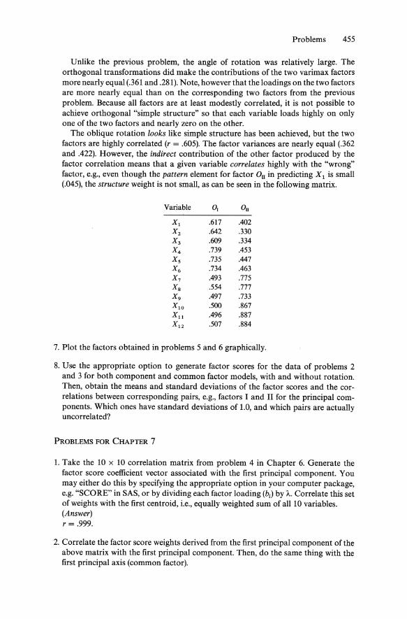
Problems 455
Unlike the previous problem, the angle of rotation was relatively large. The orthogonal transformations did make the contributions of the two varimax factors more nearly equal (.361 and .281). Note, however that the loadings on the two factors are more nearly equal than on the corresponding two factors from the previous problem. Because all factors are at least modestly correlated, it is not possible to achieve orthogonal "simple structure" so that each variable loads highly on only one of the two factors and nearly zero on the other.
The oblique rotation looks like simple structure has been achieved, but the two factors are highly correlated (r = .605). The factor variances are nearly equal (.362 and .422). However, the indirect contribution of the other factor produced by the factor correlation means that a given variable correlates highly with the "wrong" factor, e.g., even though the pattern element for factor Oil in predicting Xl is small (.045), the structure weight is not small, as can be seen in the following matrix.
Variable O. On
Xl .617 .402 X2 .642 .330
X3 .609 .334 X4 .739 .453
Xs .735 .447
X6 .734 .463 X7 .493 .775 Xs .554 .777
X9 .497 .733
XIO .500 .867 Xli .496 .887 X12 .507 .884
7. Plot the factors obtained in problems 5 and 6 graphically.
8. Use the appropriate option to generate factor scores for the data of problems 2 and 3 for both component and common factor models, with and without rotation. Then, obtain the means and standard deviations of the factor scores and the correlations between corresponding pairs, e.g., factors I and II for the principal components. Which ones have standard deviations of 1.0, and which pairs are actually uncorrelated?
PROBLEMS FOR CHAPTER 7
1. Take the 10 x 10 correlation matrix from problem 4 in Chapter 6. Generate the factor score coefficient vector associated with the first principal component. You may either do this by specifying the appropriate option in your computer package, e.g. "SCORE" in SAS, or by dividing each factor loading (hi) by A. Correlate this set of weights with the first centroid, i.e., equally weighted sum of all 10 variables. (Answer) r = .999.
2. Correlate the factor score weights derived from the first principal component of the above matrix with the first principal component. Then, do the same thing with the first principal axis (common factor).

456 Problems
(Answer) The correlation between the first principal component and scores on the first principal component is 1.0, which is inherent in a component solution. The correla-tion between the first principal axis and scores on the first principal axis depends on the method used to estimate the factor scores. The regression method (which is used by SAS and is probably the most commonly used method) led to a correlation of .989. Lack of perfect correlation is inherent in the common factor model although in many situations, such as the present, the deviation from 1.0 is trivial.
3. Take the data from problem 6 in Chapter 6. Factor variables 1 to 6 separately from variables 7 to 12. Compute the correlations between: (a) the first principal com-ponent of each data set and (b) the first principal axis of each data set. (Answer) (a) r = .538 and (b) r = .481.
4. The following pair of correlation matrices, A and B, were each derived from 50 subjects. Obtain the first principal component in each. Then, correlate the two within each correlation matrix, i.e., compute the correlation between the first principal component of A and the first principal component of B within correlation matrix A and within correlation matrix B. Finally, correlate the first principal component of A and the centroid (equally weighted linear combination) within A and do the same thing with the first principal component of B and the centroid within B.
1.000 .853 .836 .816 .818 .699 .595 .703 .767 .617
.853 1.000 .786 .789 .897 .596 .589 .686 . 707 .572
.836 .786 1.000 .763 .754 .603 .584 .634 .711 .477
.816 .789 .763 LOOO .852 .679 .522 .670 .708 .560
.818 .807 .754 .858 1.000 .691 .559 .644 .694 .610 A=
.698 .596 .606 .678 .691 1.000 .646 .581 .476 .435
.590 .589 .584 .522 .559 .646 1.000 .454 .512 .374
.702 .683 .634 .670 .644 .581 .454 1.000 .527 .530
.736 .707 .711 .708 .694 .476 .512 .527 1.000 .527
.671 .572 .477 .560 .610 .435 .374 .530 .527 1.000
1.000 .801 .764 .868 .787 .651 .767 .581 .600 .546
.801 1.000 .791 .838 .820 .644 .701 .626 . 571 .625
.764 .791 1.000 .756 .757 .628 .685 .557 .559 .694
.868 .838 .756 1.000 .811 .631 .764 .696 .691 .646
B= .787 .820 .756 .811 LOOO .560 .771 .632 .573 .558
.651 .644 .628 .631 .560 1.000 .585 .546 .412 .395
.767 .701 .685 .764 .771 .585 1.000 .584 .629 .519
.581 .626 .557 .695 .632 .546 .584 1.000 .492 .275
.600 .571 .559 .691 .573 .412 .629 .492 1.000 .401
.546 .625 .694 .646 .558 .395 .519 .275 .401 1.000
(Answer) The first principal component of A correlates .9998 with the first principal component of B within correlation matrix A and .9997 with the centroid. The first principal
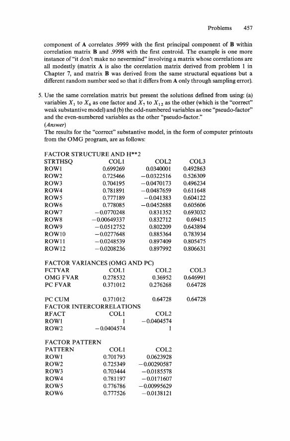
Problems 457
component of A correlates .9999 with the first principal component of B within correlation matrix Band .9998 with the first centroid. The example is one more instance of "it don't make no nevermind" involving a matrix whose correlations are all modestly (matrix A is also the correlation matrix derived from problem 1 in Chapter 7, and matrix B was derived from the same structural equations but a different random number seed so that it differs from A only through sampling error).
5. Use the same correlation matrix but present the solutions defined from using: (a) variables Xl to X6 as one factor and X 7 to X 12 as the other (which is the "correct" weak substantive model) and (b) the odd-numbered variables as one "pseudo-factor" and the even-numbered variables as the other "pseudo-factor." (Answer) The results for the "correct" substantive model, in the form of computer printouts from the OMG program, are as follows:
FACTOR STRUCTURE AND H**2 STRTHSQ CaLl COL2 ROW1 0.699269 0.0340001 ROW2 0.725466 -0.0322516 ROW3 0.704195 -0.0470173 ROW4 0.781891 -0.0487659 ROW5 0.777189 -0.041383 ROW6 0.778085 -0.0452688 ROW7 -0.0770248 0.831352 ROW8 -0.00649337 0.832712 ROW9 -0.0512752 0.802209 ROWlO -0.0277648 0.885364 ROW11 -0.0248539 0.897409 ROW12 -0.0208236 0.897992
FACTOR VARIANCES (OMG AND PC) FCTVAR CaLl COL2 OMG FV AR 0.278532 0.36952 PC FVAR 0.371012 0.276268
PC CUM 0.371012 0.64728 FACTOR INTERCORRELA nONS RFACT CaLl ROW1 1 ROW2 -0.0404574
FACTOR PATTERN PATTERN ROWI ROW2 ROW3 ROW4 ROW5 ROW6
CaLl 0.701793 0.725349 0.703444 0.781197 0.776786 0.777526
COL2 -0.0404574
1
COL2 0.0623928
-0.00290587 -0.0185578 -0.0171607
-0.00995629 -0.0138121
COL3 0.492863 0.526309 0.496234 0.611648 0.604122 0.605606 0.693032
0.69415 0.643894 0.783934 0.805475 0.806631
COL3 0.646991
0.64728
0.64728
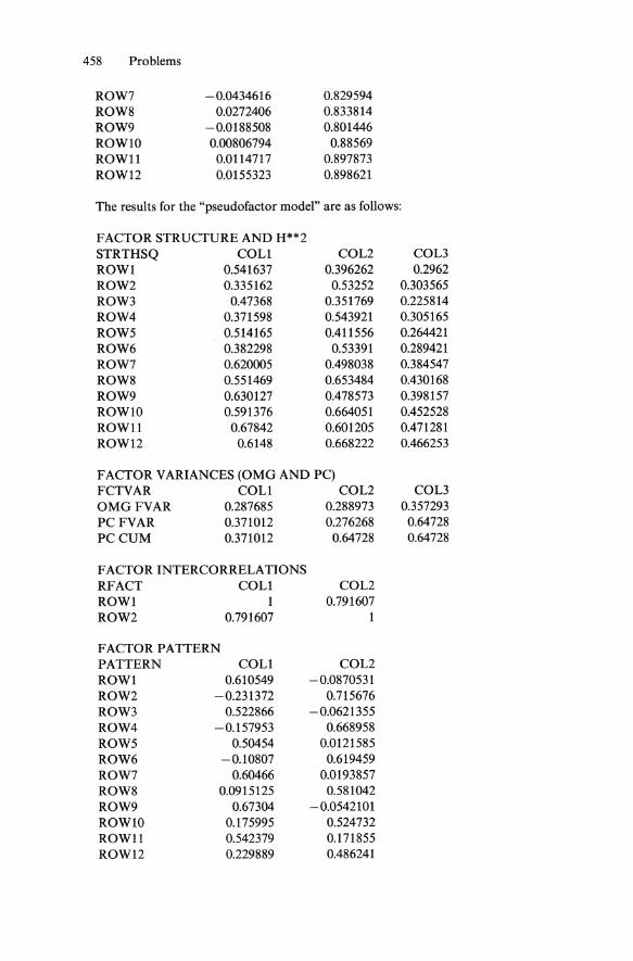
458 Problems
ROW7 ROW8 ROW9 ROWlO ROW11 ROW12
-0.0434616 0.0272406
-0.0188508 0.00806794
0.0114717 0.0155323
0.829594 0.833814 0.801446
0.88569 0.897873 0.898621
The results for the "pseudofactor model" are as follows:
FACTOR STRUCTURE AND H**2 STRTHSQ COLl ROW1 0.541637 ROW2 0.335162 ROW3 0.47368 ROW4 0.371598 ROW5 0.514165 ROW6 0.382298 ROW7 0.620005 ROW8 0.551469 ROW9 0.630127 ROWlO 0.591376 ROW 11 0.67842 ROW12 0.6148
COL2 0.396262
0.53252 0.351769 0.543921 0.411556
0.53391 0.498038 0.653484 0.478573 0.664051 0.601205 0.668222
FACTOR VARIANCES (OMG AND PC) FCTVAR COLl COL2 OMG FVAR 0.287685 0.288973 PC FV AR 0.371012 0.276268 PC CUM 0.371012 0.64728
FACTOR INTERCORRELA nONS RFACT COLl COL2 ROW1 1 0.791607 ROW2 0.791607 1
FACTOR PATTERN PATTERN COLl COL2 ROW1 0.610549 -0.0870531 ROW2 -0.231372 0.715676 ROW3 0.522866 -0.0621355 ROW4 -0.157953 0.668958 ROW5 0.50454 0.0121585 ROW6 -0.10807 0.619459 ROW7 0.60466 0.0193857 ROW8 0.0915125 0.581042 ROW9 0.67304 -0.0542101 ROW 10 0.175995 0.524732 ROW11 0.542379 0.171855 ROW12 0.229889 0.486241
COL3 0.2962
0.303565 0.225814 0.305165 0.264421 0.289421 0.384547 0.430168 0.398157 0.452528 0.471281 0.466253
COL3 0.357293
0.64728 0.64728

Problems 459
6. Now repeat the exercise with the data of problem 6, Chapter 6. (Answer)
The result for the "correct" weak substantive model is:
STRTHSQ COLl COL2 COL3 ROW1 0.705175 0.394369 0.497595 ROW2 0.720891 0.327143 0.524838 ROW3 0.698665 0.331247 0.490915 ROW4 0.778589 0.445571 0.607217 ROW5 0.774099 0.442249 0.600177 ROW6 0.776793 0.454756 0.605335 ROW7 0.446319 0.824111 0.679172 ROW8 0.501099 0.826065 0.686933 ROW9 0.45036 0.795383 0.633355 ROWlO 0.451483 0.882543 0.779634 ROW 11 0.444972 0.895637 0.804057 ROW12 0.457545 0.893292 0.798704
FACTOR VARIANCES (OMG AND PC) FCTVAR COLl COL2 COL3 OMGFVAR 0.38152 0.445532 0.642328 PC FVAR 0.497209 0.14574 0.642949 PC CUM 0.497209 0.642949 0.642949
FACTORINTERCORRELATIONS RFACT COLl COL2 ROW1 1 0.537768 ROW2 0.537768 1
FACTOR PATTERN PATTERN COLl COL2 ROW1 0.693715 0.0213115 ROW2 0.76685 -0.0851562 ROW3 0.732311 -0.0625671 ROW4 0.75826 0.0378026 ROW5 0.754456 0.0365258 ROW6 0.748784 0.0520835 ROW7 0.00441521 0.821736 ROW8 0.0800037 0.783042 ROW9 0.0318347 0.778263 ROWlO -0.032528 0.900036 ROW11 -0.0515937 0.923382 ROW12 -0.0321319 0.910571
and the pseudofactor result is
FACTOR STRUCTURE AND H**2 STRTHSQ COLl COL2 COL3 ROW1 0.658404 0.529543 0.439121 ROW2 0.487767 0.631846 0.411831
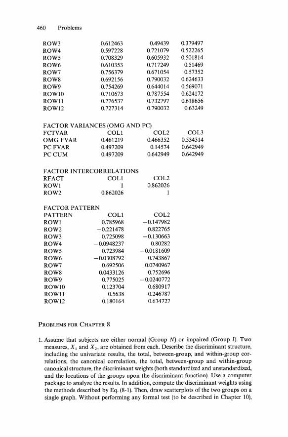
460 Problems
ROW3 0.612463 0.49439 ROW4 0.597228 0.721079 ROW5 0.708329 0.605932 ROW6 0.610353 0.717249 ROW7 0.756379 0.671054 ROW8 0.692156 0.790032 ROW9 0.754269 0.644014 ROW 10 0.710673 0.787554 ROW11 0.776537 0.732797 ROW12 0.727314 0.790032
FACTOR VARIANCES (OMG AND PC) FCTVAR COLl COL2 OMG FVAR 0.461219 0.466352 PC FVAR 0.497209 0.14574 PC CUM 0.497209 0.642949
FACTORINTERCORRELATIONS RFACT COLl ROW1 1 ROW2 0.862026
FACTOR PATTERN PATTERN COLI
0.785968 ROWI ROW2 ROW3 ROW4 ROW5 ROW6 ROW7 ROW8 ROW9 ROW10 ROW11 ROW12
-0.221478 0.725098
-0.0948237 0.723984
-0.0308792 0.692506
0.0433126 0.775025 0.123704
0.5638 0.180164
PROBLEMS FOR CHAPTER 8
COL2 0.862026
1
COL2 -0.147982
0.822765 -0.130663
0.80282 -0.0181609
0.743867 0.0740967
0.752696 -0.0240772
0.680917 0.246787 0.634727
0.379497 0.522265 0.501814
0.51469 0.57352
0.624633 0.569071 0.624172 0.618656
0.63249
COL3 0.534314 0.642949 0.642949
1. Assume that subjects are either normal (Group N) or impaired (Group I). Two measures, Xl and X 2 , are obtained from each. Describe the discriminant structure, including the univariate results, the total, between-group, and within-group correlations, the canonical correlation, the total, between-group and within-group canonical structure, the discriminant weights (both standardized and unstandardized, and the locations of the groups upon the discriminant function). Use a computer package to analyze the results. In addition, compute the discriminant weights using the methods described by Eq. (8-1). Then, draw scatterplots of the two groups on a single graph. Without performing any formal test (to be described in Chapter 10),

Problems 461
are the shapes of the two scatterplots reasonably similar except for location, i.e., are the two group homoscedastic.
Group X, X2
N 10 31 N 7 -14 N 15 -2 N 13 -11 N 13 2 N 10 8 N 2 2 N 12 24 N 24 25 N 12 2 N -4 4 N 14 39 N 10 -5 N -12 1 N 20 6 N 6 14 N 32 2 N 12 12 N 4 16 N 24 10 N 9 0 N 15 9 N 22 35 N 35 -18 N 6 -7 I 8 8 I 38 25 I -4 -3 I 5 -13 I 24 27 I -14 8 I -5 6 I 3 0 I 6 9 I 22 12 I 21 31 I 23 9 I -18 25 I -7 12 I 13 38 I 17 27 I 12 47 I -4 1 I -2 7 I -13 10 I 2 61 I -6 34 I -21 -16 I 0 13 I 17 4
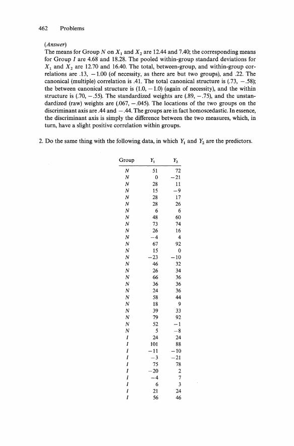
462 Problems
(Answer) The means for Group N on Xl and X2 are 12.44 and 7.40; the corresponding means for Group I are 4.68 and 18.28. The pooled within-group standard deviations for Xl and X2 are 12.70 and 16.40. The total, between-group, and within-group correlations are .13, -1.00 (of necessity, as there are but two groups), and .22. The canonical (multiple) correlation is .41. The total canonical structure is (.73, -.58); the between canonical structure is (1.0, -1.0) (again of necessity), and the within structure is (.70, -.55). The standardized weights are (.89, -.75), and the unstandardized (raw) weights are (.067, - .045). The locations of the two groups on the discriminant axis are .44 and - .44. The groups are in fact homoscedastic. In essence, the discriminant axis is simply the difference between the two measures, which, in turn, have a slight positive correlation within groups.
2. Do the same thing with the following data, in which YI and Y2 are the predictors.
Group Yt Y2
N 51 72 N 0 -21 N 28 11 N 15 -9 N 28 17 N 28 26 N 6 6 N 48 60 N 73 74 N 26 16 N -4 4 N 67 92 N 15 0 N -23 -10 N 46 32 N 26 34 N 66 36 N 36 36 N 24 36 N 58 44 N 18 9 N 39 33 N 79 92 N 52 -1 N 5 -8 I 24 24 I 101 88 I -11 -10 I -3 -21 I 75 78 I -20 2 I -4 7 I 6 3 I 21 24 I 56 46
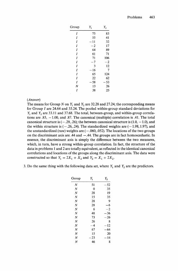
Problems 463
Group Y, Yz
I 73 83 I 55 41 I -11 32 I -2 17 I 64 89 I 61 71 I 71 106 I -7 -2 I 3 12 I -16 7 1 65 124 I 22 62 1 -58 -53 N 13 26 I 38 25
(Answe~)
The means for Group N on Y, and Y2 are 32.28 and 27.24; the corresponding means for Group I are 24.64 and 35.24. The pooled within-group standard deviations for Y, and Y2 are 33.11 and 37.68. The total, between-group, and within-group correlations are .85, -1.00, and .87. The canonical (multiple) correlation is .41. The total canonical structure is ( - .29, .26); the between canonical structure is (1.0, -1.0), and the within structure is ( - .26, .24). The standardized weights are ( -1.98, 1.97), and the unstandardized (raw) weights are ( - .060, .052). The locations of the two groups on the discriminant axis are .44 and - .44. The groups are in fact homoscedastic. In essence, the discriminant axis is simply the difference between the two measures, which, in turn, have a strong within-group correlation. In fact, the structure of the data in problems 1 and 2 are totally equivalent, as reflected in the identical canonical correlations and locations of the groups along the discriminant axis. The data were constructed so that Yr = 2X, + X2 and Y2 = X, + 2X2 •
3. Do the same thing with the following data set, where Y, and Y2 are the predictors.
Group Y, Yz
N 51 -52 N 0 35 N 28 19 N 15 35 N 28 9 N 28 -6 N 6 -2 N 48 -36 N 73 -26 N 26 8 N -4 -12 N 67 -64 N 15 20 N -23 -14 N 46 8

464 Problems
Group Yl Y2
N 26 -22 N 66 28 N 36 -12 N 24 -28 N 58 4 N 18 9 N 39 -3 N 79 -48 N 52 71 N 5 20 I 24 -8 I 101 -12 I -11 2 I -3 31 I 75 -30 I -20 -30 I -4 -17 I 6 3 I 21 -12 I 56 -2 I 73 -41 I 55 5 I -11 -68 I -2 -31 I 64 -63 I 61 -37 I 71 -82 I -7 -6 I 3 -16 I -16 -33 I 65 -120 I 22 -74 I -58 11 I 13 -26 I 38 9
(Answer) The means for Group N on Y1 and Y2 are 32.28 and - 2.36; the corresponding means for Group I are 24.64 and 25.88. The pooled within-group standard deviations for Y1 and Y2 are 33.11 and 32.48. The total, between-group, and within-group correlations are -.26, -1.00, and -.33, respectively. The canonical (multiple) correlation is .41. The total canonical structure is (.29, .85); the between canonical structure is (1.0, - 1.0), and the within canonical structure is (.26, .83). The standardized weights are .60, 1.08, and the unstandardized (raw) weights are .02, .03. The locations of the two groups on the discriminant axis are .44 and - .44. The groups are in fact homoscedastic. In essence, the discriminant axis is simply the sum the two measures, which, in turn, have a strong within-group correlation. In fact, the structure of the data in problems 1 and 3 are totally equivalent, as reflected in the identical canonical correlations and locations of the groups along the discriminant axis. The data were constructed so that Y1 = 2X 1 + X 2 and Y2 = Xl - 2X 2·

Problems 465
4. Do the same thing with the following data set, where Y1 and Yz are the predictors.
Group Y1 Y2
N 10 31 N 7 -14 N 15 -2 N 13 -11 N 13 2 N 10 8 N 2 2 N 12 24 N 24 25 N 12 2 N -4 4 N 14 39 N 10 -5 N -12 1 N 20 6 N 6 14 N 32 2 N 12 12 N 4 16 N 24 10 N 9 0 N 15 9 N 22 35 N 35 -18 N 6 -7 I 8 9 I 38 43 I -4 -13 I 5 -33 I 24 47 I -14 9 I -5 5 I 3 -7 I 6 11 I 22 17 I 21 55 I 23 11 I -18 43 I -7 17 I 13 69 I 17 47 I 12 87 I -4 -5 I -2 7 I -13 13 I 2 115 I -6 61 I -21 -39 I 0 19 I 17
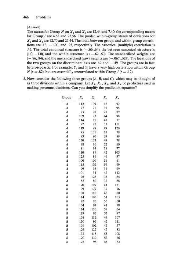
466 Problems
(Answer) The means for Group N on Xl and X 2 are 12.44 and 7.40; the corresponding means for Group I are 4.68 and 23.56. The pooled within-group standard deviations for Xl and X 2 are 12.70 and 27.44. The total, between-group, and within-group correlations are .13, -1.00, and .25, respectively. The canonical (multiple) correlation is .45. The total canonical structure is ( - .66, .64); the between canonical structure is (1.0, - 1.0), and the within structure is (- .62, .60). The standardized weights are (- .86, .84), and the unstandardized (raw) weights are (- .067, .029). The locations of the two groups on the discriminant axis are .49 and - .49. The groups are in fact heteroscedastic. For example, Y;. and Y2 have a very high correlation within Group N (r = .82), but are essentially uncorrelated within Group I (r = .12).
5. Now, consider the following three groups (A, B, and C), which may be thought of as three divisions within a company. Let Xl' X 2 , X 3 , and X4 be predictors used in making personnel decisions. Can you simplify the prediction equation?
Group XI X 2 X3 X 4
A 112 109 45 92 A 77 91 35 95 A 73 98 23 89 A 109 93 44 98 A 114 85 41 77 A 97 91 33 111 A 119 98 49 120 A 95 105 63 79 A 93 80 39 89 A 130 103 49 78 A 98 90 52 60 A 81 94 38 77 A 110 89 42 105 A 125 86 46 97 A 100 100 36 61 A 115 102 59 99 A 99 93 34 99 A 101 91 42 142 A 96 126 38 84 A 82 80 32 88 B 120 109 41 151 B 99 127 37 76 B 108 110 46 80 B 114 105 51 103 B 82 95 55 60 B 134 94 41 78 B 114 120 59 64 B 119 96 52 97 B 158 112 49 107 B 130 96 42 111 B 101 102 45 57 B 126 127 47 83 B 132 118 55 108 B 120 130 53 66 B 125 98 46 82

Problems 467
Group X, X2 X3 X4
B 110 108 33 71 B 173 94 64 90 B 104 111 60 48 B 91 82 33 99 B 144 100 46 79 C 100 117 48 65 C 111 109 53 51 C 101 112 52 96 C 143 102 71 78 C 140 108 49 113 C 125 114 47 81 C 130 106 52 92 C 104 113 62 70 C 149 92 49 91 C 130 110 61 81 C 117 113 63 121 C 126 96 54 87 C 128 100 51 88 C 122 130 54 85 C 112 126 45 73 C 137 91 75 79 C 125 101 39 77 C 136 116 69 97 C 129 93 57 84 C 139 92 59 78
(Answer) The means for Group A are 101.30, 95.20, 42.00, and 92.00; the means for Group B are 120.20, 106.70,47.75, and 85.50, and the means for Group Care 125.20, 107.05, 55.50, and 84.35. The pooled within-group standard deviations are 17.46, 11.63,9.06, and 19.73. The total, between-group, and within-group correlation matrices are as follows:
['00 .13 .53
15l .13 1.00 .24 -.17 T=
.53 .24 1.00 -.15
.15 -.17 -.15 1.00
[ 100 .98 .92
-~l .98 1.00 .83 -.99 B=
.92 .83 1.00 -.89
-.99 -.99 -.89 1.00
[ 100 -.12 .38 29l -.12 1.00 .07 -.11 W=
.38 .06 1.00 -.08
.29 -.11 -.08 1.00
The two canonical correlations are .67 and .28. Since the first one accounts for 90% of the total variance, the structure is concentrated so only the first one needs be

468 Problems
considered (significance tests, considered in Chapter 10, will confirm this point). The total structure is (.76, .63, .73, -.25); the between structure is (.99, .98, .93, - .99), and the within structure is (.66, .52, .64, - .19). The standardized canonical coefficients are (.80, .60, .36, - .30), and the raw canonical coefficients are (.04, .05, .03, and - .02). Group A is located at - 1.23 on the axis, Group B is located at .36, and Group C is located at .86. Various simplifications are possible. For example, the canonical correlation obtain using the sum of Xl, X 2 , and X3 with equal weights is .65, implying little would be lost with this equation.
6. Now, perform the same analysis upon the following data.
Group Xl X2 X3 X4
A 104 93 49 34 A 98 93 40 29 A 103 104 28 24 A 112 99 35 41 A 88 86 35 49 A 113 109 56 59 A 107 80 38 40 A 83 105 44 39 A 102 88 30 44 A 76 84 32 21 A 91 98 50 46 A 124 110 29 36 A 85 113 40 39 A 117 108 42 38 A 104 96 44 67 A 151 102 32 24 A 92 91 32 37 A 156 99 28 52 A 90 78 37 29 A 102 96 35 34 B 100 109 20 32 B 125 118 41 31 B 120 115 49 41 B 151 136 46 37 B 148 117 34 50 B 111 102 25 35 B 133 117 56 60 B 156 137 40 57 B 112 112 28 30 B 115 112 26 30 B 117 127 60 70 B 109 83 18 41 B 119 106 50 37 B 117 97 42 29 B 100 103 36 18 B 136 114 32 49 B 132 108 35 39 B 143 117 33 38 B 112 103 35 33 B 115 120 43 26
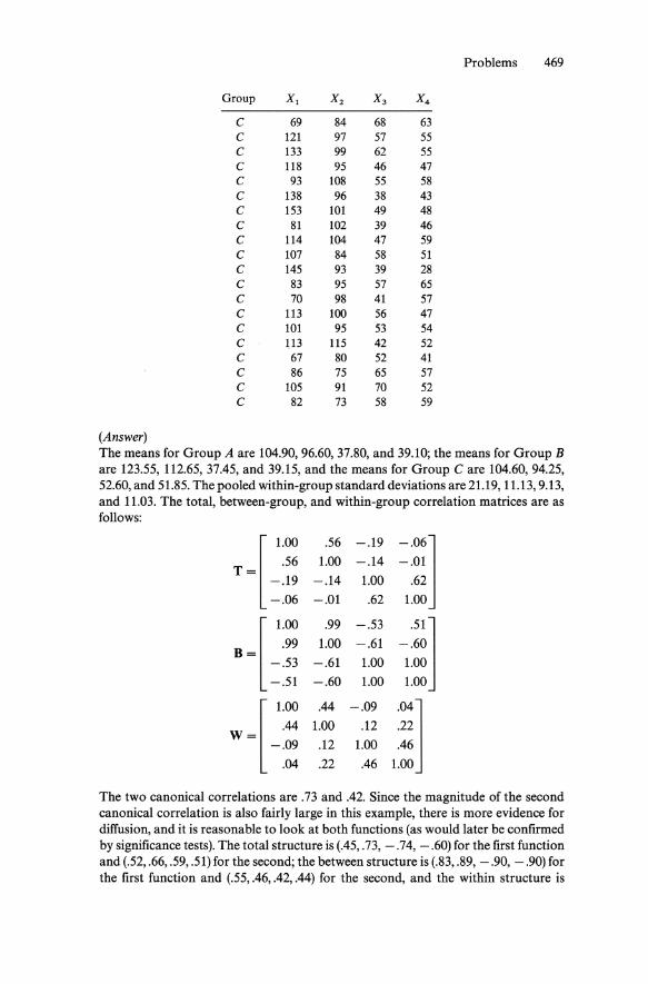
Problems 469
Group Xl X2 X3 X4
C 69 84 68 63 C 121 97 57 55 C 133 99 62 55 C 118 95 46 47 C 93 108 55 58 C 138 96 38 43 C 153 101 49 48 C 81 102 39 46 C 114 104 47 59 C 107 84 58 51 C 145 93 39 28 C 83 95 57 65 C 70 98 41 57 C 113 100 56 47 C 101 95 53 54 C 113 115 42 52 C 67 80 52 41 C 86 75 65 57 C 105 91 70 52 C 82 73 58 59
(Answer) The means for Group A are 104.90,96.60,37.80, and 39.10; the means for Group B are 123.55, 112.65, 37.45, and 39.15, and the means for Group Care 104.60, 94.25, 52.60, and 51.85. The pooled within-group standard deviations are 21.19,11.13,9.13, and 11.03. The total, between-group, and within-group correlation matrices are as follows:
r LOO
.56 -.19 -06l .56 1.00 -.14 -.01 T=
-.19 -.14 1.00 .62
-.06 -.01 .62 1.00
r LOO
.99 -.53
51l .99 1.00 -.61 -.60 B=
-.53 -.61 1.00 1.00
-.51 -.60 1.00 1.00
r LOO .44 -.09
Ml .44 1.00 .12 .22 W=
.12 1.00 .46 -.09
.04 .22 .46 1.00
The two canonical correlations are .73 and .42. Since the magnitude of the second canonical correlation is also fairly large in this example, there is more evidence for diffusion, and it is reasonable to look at both functions (as would later be confirmed by significance tests). The total structure is (.45, .73, - .74, - .60) for the first function and (.52, .66, .59, .51) for the second; the between structure is (.83, .89, - .90, - .90) for the first function and (.55, .46, .42, .44) for the second, and the within structure is

470 Problems
(.33,.62, -.63, -.47) for the first function and (.51,.75,.67,.53) for the second. The standardized canonical coefficients are ( - .05, .98, - .67, - .44) for the first function and (.36,.62,.71,.14) for the second, and the raw canonical coefficients are (.00,.07, - .06, - .04) for the first function and (.02, .04, .06, .02) for the second. Group A is located at (.11, -.64), Group B is located at (1.23,.36), and Group C is located at (-1.33,.27). The first function is thus essentially X 2 - X3 + X 4 • Group B obtains high scores (X2 is large compared to X3 and X 4 ) Group C obtains low scores, and Group A obtains average scores. The second function is essentially the sum with variables X 2 and X3 weighted more heavily (which does not make much of a difference). Group A obtains very low scores and Groups Band C obtain scores of about the same magnitude which are modestly high.
PROBLEMS FOR CHAPTER 9
1. Assume that a signal detection study gave rise to the following six pairs of hit rates and false alarm rates. Draw the ROC curves in both probability and normal curve form. In addition, compute the likelihood ratios associated with each criterion. Do the data fit a particular model?
Criterion 2 3 4 5 6
p(Yjs) .977 .933 .726 .500 .159 .040 p(Yjn) .960 .894 .637 .401 .106 .023
(Answer)
Criterion p(Yjs) p(Yjn) z(Yjs) z(Yjn) l(zj)
.977 .960 2.00 1.75 .628 2 .933 .894 1.50 1.25 .710 3 .726 .637 .60 .35 .888 4 .500 .401 .00 -.25 1.031 5 .159 .106 -1.00 -1.25 1.322 6 .040 .023 -1.75 -2.00 1.592
The data fit an equal variance Gaussian model.
2. Perform the same analysis upon the following data.
Criterion 2 3 4 5 6
p(Yjs) .841 .742 .681 .618 .520 .347 p(Yjn) .841 .692 .579 .500 .308 .159
(Answer)
Criterion p(Yjs) p(Yjn) z(Yjs) z(Yjn) l(z;)
.841 .841 1.00 1.00 1.000 2 .742 .692 .65 .50 .818 3 .681 .579 .47 .20 .913 4 .618 .500 .30 .00 .954 5 .520 .308 .05 -.50 1.131 6 .347 .159 -.40 -1.00 1.521
The data fit an unequal variance Gaussian model.
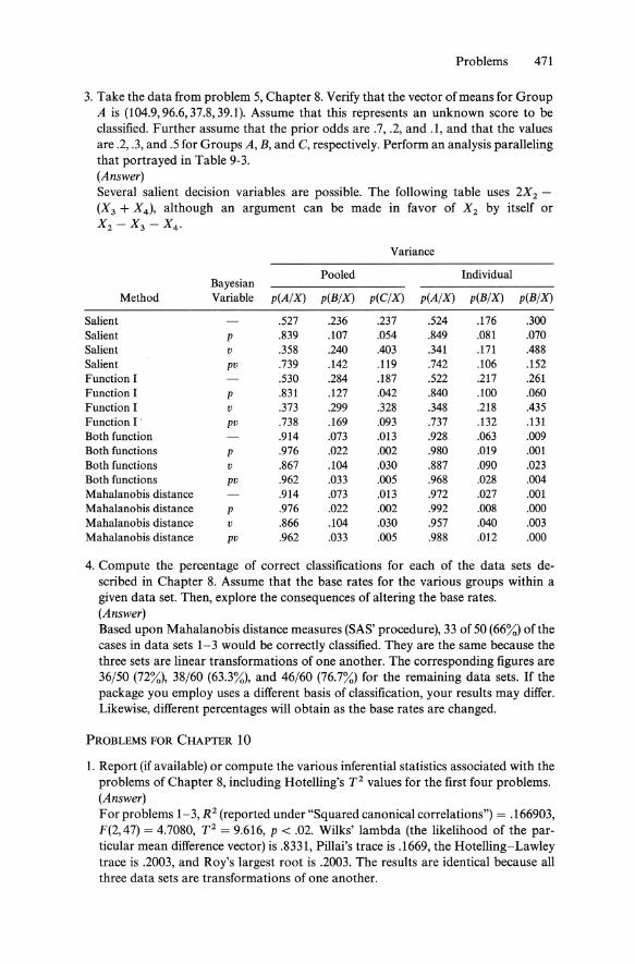
Problems 471
3. Take the data from problem 5, Chapter 8. Verify that the vector of means for Group A is (104.9,96.6,37.8,39.1). Assume that this represents an unknown score to be classified. Further assume that the prior odds are .7, .2, and .1, and that the values are .2, .3, and .5 for Groups A, B, and C, respectively. Perform an analysis paralleling that portrayed in Table 9-3. (Answer) Several salient decision variables are possible. The following table uses 2X2 -
(X3 + X 4 ), although an argument can be made in favor of X 2 by itself or X 2 - X3 - X 4 ·
Variance
Bayesian Pooled Individual
Method Variable peA/X) pCB/X) p(C/X) peA/X) pCB/X) pCB/X)
Salient .527 .236 .237 .524 .176 .300 Salient p .839 .107 .054 .849 .081 .070 Salient v .358 .240 .403 .341 .171 .488 Salient pv .739 .142 .119 .742 .106 .152 Function I .530 .284 .187 .522 .217 .261 Function I p .831 .127 .042 .840 .100 .060 Function I v .373 .299 .328 .348 .218 .435 Function I' pv .738 .169 .093 .737 .132 .131 Both function .914 .073 .013 .928 .063 .009 Both functions p .976 .022 .002 .980 .019 .001 Both functions v .867 .104 .030 .887 .090 .023 Both functions pv .962 .033 .005 .968 .028 .004 Mahalanobis distance .914 .073 .013 .972 .027 .001 Mahalanobis distance p .976 .022 .002 .992 .008 .000 Mahalanobis distance v .866 .104 .030 .957 .040 .003 Mahalanobis distance pv .962 .033 .005 .988 .012 .000
4. Compute the percentage of correct classifications for each of the data sets described in Chapter 8. Assume that the base rates for the various groups within a given data set. Then, explore the consequences of altering the base rates. (Answer) Based upon Mahalanobis distance measures (SAS' procedure), 33 of 50 (66%) of the cases in data sets 1-3 would be correctly classified. They are the same because the three sets are linear transformations of one another. The corresponding figures are 36/50 (72%), 38/60 (63.3%), and 46/60 (76.7%) for the remaining data sets. If the package you employ uses a different basis of classification, your results may differ. Likewise, different percentages will obtain as the base rates are changed.
PROBLEMS FOR CHAPTER 10
1. Report (if available) or compute the various inferential statistics associated with the problems of Chapter 8, including Rotelling's T2 values for the first four problems. (Answer) For problems 1-3, R2 (reported under "Squared canonical correlations") = .166903, F(2,47) = 4.7080, T2 = 9.616, p < .02. Wilks' lambda (the likelihood of the particular mean difference vector) is .8331, Pill ai's trace is .1669, the Rotelling-Lawley trace is .2003, and Roy's largest root is .2003. The results are identical because all three data sets are transformations of one another.

472 Problems
For problem 4, R2 = .200193, F(2,47) = 5.8821, T2 = 12.014, P < .01. Wilks' lambda is .7998, Pill ai's trace is .2002, the Hotelling-Lawley trace is .2503, and Roy's largest root is .2503.
For problem 5, the two squared canonical correlations are .4556 and .0824 (neither are R2 values since there are three groups and therefore only two sets of dummy or other codes are needed), F = 5.6019 and 1.6467, p < .001 and ns. The two tests are respectively based upon 8 and 108 and 3 and 55 df Wilks' lambda is .4995, Pillai's trace is .5381, the Hotelling-Lawley trace is .9269, and Roy's largest root is .8371. Thus, the first dimension of discrimination is significant, but the second is not.
For problem 6, the two squared canonical correlations are .5366 and .1778, F(8, 108) = 8.37 and F(3,55) = 3.96, ps < .001 and .01. Wilks' lambda is .3810, Pill ai's trace is .7144, the Hotelling-Lawley trace is 1.3743, and Roy's largest root is 1.1580. Thus, both dimensions of discrimination are significant.
2. Students were taught a computer language by one of three different methods. Method 1 consisted of using the large university mainframe computer, method 2 consisted of using the "Banana" personal computer, and method 3 consisted of using both. Two different instructors (A and B) taught 10 students by each of the three methods. The data obtained from the students consisted of SAT scores as an index of general academic ability, two hour examinations and a final examination. There were a possible 75 points on each of the hour examinations and 150 on the final. Use a MANOVA to test the effects of method, differences between the two instructors, and the the effects of their interaction upon the vector of examination scores, ignoring, for the moment, SAT scores. The data are as follows:
Method Instructor SAT Exam 1 Exam 2 Final
A 396 30 34 86 A 371 >15 20 67 A 498 19 31 43 A 598 37 30 85 A 542 38 24 79 A 556 29 26 63 A 673 42 34 94 A 649 35 42 123 A 459 25 16 75 A 730 53 44 95 B 487 47 45 123 B 270 29 38 96 B 539 49 42 104 B 557 56 41 112 B 384 43 48 91 B 672 57 57 138 B 520 44 45 88 B 690 48 46 103
1 B 617 49 73 95 1 B 375 32 31 83 2 A 634 51 53 82 2 A 435 42 65 74 2 A 530 49 57 92 2 A 361 42 44 102

Problems 473
Method Instructor SAT Exam 1 Exam 2 Final
2 A 293 31 39 110 2 A 469 57 43 83 2 A 527 53 65 119 2 A 407 46 40 104 2 A 632 70 60 98 2 A 572 56 45 84 2 B 307 39 45 91 2 B 454 52 66 95 2 B 556 56 60 111 2 B 595 58 74 107 2 B 457 52 45 93 2 B 437 46 53 67 2 B 537 73 45 129 2 B 545 51 61 120 2 B 231 27 23 66 2 B 492 62 48 92 3 A 451 57 68 119 3 A 333 57 59 129 3 A 564 59 66 127 3 A 677 82 66 164 3 A 587 73 63 121 3 A 524 68 67 117 3 A 533 69 61 126 3 A 382 55 62 146 3 A 384 70 46 120 3 A 437 66 62 144 3 B 579 48 48 126 3 B 462 50 34 107 3 B 601 57 42 102 3 B 558 53 62 107 3 B 589 52 62 90 3 B 417 53 30 150 3 B 513 53 41 78 3 B 669 62 55 138 3 B 511 54 34 114 3 B 482 57 33 118
(Answer) The effect of method is highly significant, which implies that the vectors for method 1 (38.85,38.35,92.15), method 2 (50.65,51.55,95.95), and method 3 (59.75,53.05, 122.15) can be assumed different. Wilks' lambda is .4085, which corresponds to an F ratio of 9.78 with 6 and 104 df. Pillai's trace is .6809 which corresponds to an F ratio of 9.12 with 6 and 106 df. The Hotelling-Lawley trace is 1.2285 which corresponds to an F ratio of 10.44 with 6 and 102 df, and Roy's largest root is 1.012, which corresponds (approximately) to an F ratio of 17.88 with 3 and 53 df. All effects are significant well beyond the .001 level.
The structure is fairly well concentrated with the first eigenvalue accounting for 82.4% of the variance and the second accounting for 17.6%. The discriminant axis is (.0094, .0033, .0024) which means that groups are most different on the first test once all test scores are adjusted for each other. Univariate tests indicated that all
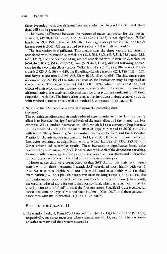
474 Problems
three dependent variables different from each other well beyond the .001 level (these data will not be presented).
The overall difference between the vectors of mean test scores for the two instructors, (49.20,47.73,102.36) and (50.30,47.57,104.47) is not significant. Wilks' lambda is .9939; Pill ai's trace is .0060; the Hotelling-Lawley trace is .0061, and Roy's largest root is .0061. All correspond to F ratios < 1.0 with df = 3 and 52.
The interaction is significant. This means that the three vectors individually associated with instructor A, which are (32.3,30.1,81.0), (49.7,51.1,94.8), and (65.6, 62.0,131.3), and the corresponding vectors associated with instructor B, which are (45.4,46.6,103.3), (51.6,52.0,97.1), and (53.9,44.1,113.0), differed following correction for the two main effect vectors. Wilks' lambda is .6170, F(6, 104) = 4.73; Pillai's trace is .3823, F(6, 106) = 4.19, the Hotelling-Lawley trace is .6204, F(6, 102) = 5.27, and Roy's largest root is .6199, F(3, 53) = 10.95, (all ps < .001). The first eigenvector accounted for 99.91% of the total variance so the interaction may be regarded as concentrated. The eigenvector is (.0040, .0087, .0024), which means that the joint effects of instructor and method are seen most strongly on the second examination, although univariate analyses indicated that the interaction is significant for all three dependent variables. The interaction reveals that instructor A does relatively poorly with method 1 and relatively well on method 3, compared to instructor B.
3. Now, use the SAT score as a covariate upon the preceding data. (Answer) The covariance adjustment strongly reduced experimental error so that its primary effect is to increase the significance levels of the main effect and the interaction. For example, Wilks' lambda decreased to .1544, which led to a corresponding increase in the associated F ratio for the main effect of Type of Method to 26.26, p < .001, with 6 and 102 df Similarly, Wilks' lambda decreased to .2625 and the associated F ratio for the interaction increased to 16.18, p < .001. However, the main effect of Instructor remained nonsignificant with a Wilks' lambda of .9858, F(3,51) < 1. Other criteria led to similar results. These increases in significance levels arise because the pretest measure (SAT) is correlated with each of the dependent variables. Consequently, removing its effect prior to assessing the main effects and interaction reduces experimental error, the goal of any covariance analysis.
However, the data were constructed so that SAT did not correlate to an equal extent with all three measures. Instead, SAT correlated most highly with test 1 (r = .78), next most highly with test 2 (r = .62), and least highly with the fmal examination (r = .32, a plausible outcome since the longer one is in the course, the more information specific to the course would determine performance). As a result, the error is reduced more for test 1 than for the final, which, in turn, meant that the discriminant axis is "tilted" toward the first test more. Specifically, the eigenvector associated with the Type of Method effect is (.0205, .0031, .0020), and the eigenvector associated with the Interaction is (.0181, .0123, .0005).
PROBLEMS FOR CHAPTER 11
1. Three individuals, A, B, and C, obtain vectors of (44,17,12), (34,12,8), and (50,15,8), respectively, on three measures whose means are 40, 15, and 12. The variancecovariance matrix of the three measures is:
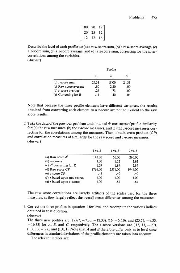
Problems 475
[100 20 12] 20 25 12 12 12 16
Describe the level of each proftle as: (a) a raw-score sum, (b) a raw-score average, (c) a z-score sum, (c) a z-score average, and (d) a z-score sum, correcting for the intercorrelations among the variables. (Answer)
Profile
A B C
(b) z-score sum 24.33 18.00 24.33 (c) Raw score average .80 -2.20 .00 (d) z-score average .26 -.73 .00 (e) Correcting for R .14 -.40 .04
Note that because the three proftle elements have different variances, the results obtained from converting each element to a z-score are not equivalent to the raw score results.
2. Take the data of the previous problem and obtained d2 measures of proftle similarity for: (a) the raw measures, (b) the z-score measures, and (c) the z-score measures correcting for the correlations among the measures. Then, obtain cross-product (CP) and correlation measures of similarity for the raw score and z-score measures. (Answer)
1 vs. 2 1 vs.3 2 vs. 3
(a) Raw score d2 141.00 56.00 265.00 (b) z-score d2 3.00 1.52 2.92 (c) d2 correcting for R 1.69 1.89 2.89 (d) Raw score CP 1796.00 2551.00 1944.00 (e) z-score CP -.48 .40 .40 (f) r based upon raw scores 1.00 1.00 1.00 (g) r based upon z-scores 1.00 .87 .87
The raw score correlations are largely artifacts of the scales used for the three measures, as they largely reflect the overall mean differences among the measures.
3. Correct the three profiles in question 1 for level and recompute the various indices obtained in that question. (Answer) The three new proftles are (19.67, -7.33, -12.33), (16, -6,10), and (25.67, -9.33, -16.33) for A, B, and C, respectively. The z-score versions are (.13, .13, - .27), (.13,.13, -.27), and (1,0,1). Note that A and B therefore differ only as to level once differences in standard deviations of the proftle elements are taken into account.
The relevant indices are:

476 Problems
Profile
A B C
(a) Raw score sum 0.00 0.00 0.00 (b) z-score sum 0.00 0.00 0.00 (c) Raw score average 0.00 0.00 0.00 (d) z-score average 0.00 0.00 0.00 (e) Correcting for R .00 -.00 .04
Note that uncorrected "elevation" measures are .0 once a correction for level is introduced.
4. Now, compute d2 , CP, and correlation-based similarity measures for the levelcorrected measures. (Answer)
1 vs. 2 1 vs. 3 2 vs. 3
(a) Raw score d2 20.67 56.00 144.67 (b) z·score dZ 0.00 1.31 1.31 (c) d2 correcting for R .00 1.84 1.84 (d) Raw score CP 482.00 774.67 630.00 (e) z·score CP .11 .40 .40 (f) r based upon raw scores 1.00 1.00 1.00 (g) r based upon z·scores 1.00 .87 .87
The correlation measures do not change from the original (nonleve1-corrected case) because they were insensitive to level to begin with.
5. The following 45 profiles were constructed so that the first 15 belonged to one class, the next 15 to a second class, and the last 15 to a third class. Profiles in the second class were higher than profiles in the first class on the first three measures (Xl to X 3 )
but equivalent on the last three measures (X4 to X6)' The converse is true for profiles in the third class. Use a suitable clustering program to determine groupings. Do the various measures of fit change abruptly at three clusters? How well does a threecluster solution reconstruct the actual classes?
Xl Xz X3 X4 Xs X6
49 51 40 50 53 57 53 45 55 45 53 56 50 52 54 47 40 45 43 42 40 54 53 50 57 61 44 54 60 51 40 47 45 60 49 46 48 42 41 48 35 35 56 47 50 57 51 55 63 52 60 57 53 57 46 63 55 50 56 52 48 46 51 52 48 47 60 51 61 70 71 71 44 44 44 42 43 37 74 88 74 52 60 54

Problems 477
XI X2 X3 X4 Xs X6
49 40 56 47 50 46 55 63 50 42 48 40 67 57 68 51 43 45 82 76 83 64 61 55 83 73 77 65 57 61 65 70 79 69 60 59 79 75 78 71 62 71 63 65 64 42 43 43 61 62 72 73 57 66 67 74 75 60 56 72 66 63 71 52 52 52 74 61 66 41 45 47 73 57 74 36 43 46 73 63 73 50 49 45 82 83 79 61 67 66 70 ,62 67 55 59 49 41 52 43 85 87 90 62 61 63 76 80 72 56 56 59 67 63 66 52 69 50 79 85 77 57 58 66 56 74 60 55 48 54 81 73 76 62 65 54 80 77 81 61 56 63 56 75 60 47 56 48 60 54 59 43 58 46 73 74 n 61 55 57 77 73 74 52 40 45 72 64 69 35 44 37 59 57 68 60 55 55 72 66 63 51 63 60 58 62 63
(Answer) Your results may differ because of differences in the algorithm. Using Ward's method, 12 members of Group 3 were placed in one cluster along with 1 member of Group 1; 13 members of Group 1, 1 member of Group 2, and 3 members of Group 3 were placed into a second cluster, and 14 members of Group 2 and 1 member of Group 1 were placed in the third cluster. The RMS standard deviations associated with 1 through 6 clusters are: 12.18, 10.89,8.72,7.37,7.74, and 6.45 so the increase in homogeneity in going from two to three categories is relatively large. Likewise, the associated semipartial r2 values were .31, .29 .. 10, .04, .04, and -.02. Finally, the R2 values were .00, .31, .59, .69, .73, and .77. The latter two measures thus tell the same story.
6. Assume you had analyzed blood samples of 90 subjects to determine the levels of three hormones, HI' H 2 , and H3 • Also assume that you had obtained systolic blood pressure (S), diastolic blood pressure (D), and pulse rate measures (P) on these same subjects. What relations exist between these hypothetical hormones, on the onehand, and the blood pressure and pulse rate measures, on the other? The data are as follows:
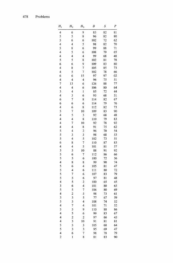
478 Problems
HI Hz H3 D S P
4 6 9 83 82 81 5 5 8 96 82 80 5 6 6 102 72 62 4 4 5 98 82 70 5 8 6 99 88 71 4 5 6 108 79 65 4 4 4 99 68 48 5 5 8 102 81 78 6 6 9 109 83 80 4 8 7 105 85 73 4 5 7 102 78 66 6 6 15 97 97 02 4 4 4 96 75 51 7 13 6 126 88 77 4 4 6 106 80 64 3 4 1 85 72 44 4 3 6 93 68 51 6 7 8 114 82 67 6 6 6 114 79 76 4 6 8 112 82 73 5 7 10 109 83 90 4 5 3 92 68 48 4 4 8 110 79 83 4 7 10 92 78 92 4 4 8 91 75 62 5 4 2 96 70 54 5 3 3 98 68 53 5 4 5 102 73 51 6 8 7 110 87 83 4 4 5 101 81 57 3 5 10 88 91 92 5 6 7 112 86 66 5 5 6 100 72 56 4 8 8 99 90 74 5 6 4 105 81 47 5 4 6 111 80 72 5 7 6 107 83 79 5 5 6 97 81 48 4 5 2 100 65 45 3 6 4 101 80 65 5 5 7 106 80 69 4 2 5 98 73 61 3 3 5 77 67 59 5 5 4 108 74 52 4 7 4 101 71 52 5 5 9 110 88 86 4 5 6 99 83 67 4 2 2 97 66 43 4 3 10 91 81 81 5 5 3 105 68 64 5 3 3 95 69 47 4 6 7 98 78 79 2 8 81 83 90
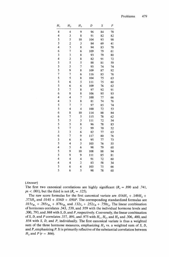
Problems 479
HI H2 H3 D S P
4 4 9 96 84 78 4 3 8 91 82 82 5 5 10 104 93 98 3 2 3 84 69 41 4 3 8 94 83 78 6 7 6 109 79 61 3 3 8 93 79 80 4 3 8 82 91 72 5 5 5 88 81 59 5 5 7 95 74 74 5 9 8 109 87 92 7 7 6 116 85 76 5 5 8 104 75 63 5 6 5 111 75 60 5 6 6 109 76 62 5 7 8 97 92 91 6 8 8 106 95 93 4 4 7 100 77 66 4 3 8 81 74 76 5 7 7 97 85 74 5 4 4 100 72 53 6 8 10 114 88 84 6 7 5 115 78 62 5 5 5 111 72 54 5 5 8 96 78 83 5 7 5 99 70 52 3 3 6 82 77 63 6 7 9 117 80 76 5 6 6 95 77 73 5 4 5 105 76 55 4 5 6 98 79 60 5 9 10 108 88 94 5 9 9 111 85 81 4 4 4 91 72 60 4 4 2 83 58 34 5 6 6 103 75 66 5 6 5 98 78 60
(Answer) The first two canonical correlations are highly significant (Rc = .890 and .741, ps < .001), but the third is not (Rc = .125).
The raw score formulas for the first canonical variate are .016H1 + .149H2 + .373H3 and .014S + .034D + .050P. The corresponding standardized formulas are .015zH , + .285zH2 + .878zH , and .132zs + .252zD + .750zp • The linear combination of hormones correlates .343, .539, and .959 with the individual hormone levels and .300, .793, and .868 with S, D, and P, respectively. Conversely, the linear combination of S, D, and P correlates .337, .891, and .975 with H 1 , H2 , and H3 and .306, .480, and .854 with S, D, and P, individually. The first canonical variate is thus a weighted sum of the three hormone measures, emphasizing H3 vs. a weighted sum of S, D, and P, emphasizing P. It is primarily reflective ofthe substantial correlation between H3 and P (r = .866).

480 Problems
The raw score formulas for the second canonical variate are .801H1 + .192Hz -.199H3 and .103S + .017D - .031P. The corresponding standardized formulas are .728zH1 + .368zH2 - .467zH3 and .978zs + .127zD - .453zp • The linear combination of hormones correlates .874, .687, and - .238 with the individual hormone levels and .692, .032, and -.132 with S, D, and P, respectively. Conversely, the linear combination of S, D, and P correlates .934, .043, and -.179 with H 1 , Hz, and H3 and .648 .509, and - .176 with S, D, and P, individually. The first canonical variate is thus a weighted sum of Hl and Hz, minus H 3 , emphasizing Hl vs. basically the weighted differences of S - P, emphasizing S.
The two linear combinations of hormones individually account for 62.4% and 26.7% of their own variance, for a total of 89.1%. They also account for 49.4% and 14.6% of the variance in S, D, and P, for a total of 64.0%. Conversely, the two linear combinations of S, D, and P account for 71.8% and 23.7% oftheir own variance, for a total of 95.5%. Likewise, they account for 56.9% and 13.0% of the variance among the hormone measures, for a total of 69.9%.
PROBLEMS FOR CHAPTER 12
1. Suppose that tests A, B, and C have reliability coefficients of .8, .5, and .3. What is the maximum correlation each can have with some external criterion. (Answer) The maximum correlations (equal to the reliability indices) are .89, .71, and .55, which are the respective square roots of the reliability coefficients.
2. Now, suppose that tests D, E, and F correlate .4, .5, and .6 with some external criterion. What is the minimum value of their associated reliability coefficients can assume. (Answer) Assume that the above values are lower bounds on the reliability index. The reliability coefficients would be .16, .25, and .36, i.e., the squares of the obtained correlations.
3. A five-item test gave rise to the following variance-covariance matrix. Compute the reliability of the test.
LOOOO .4301 .4230 .2786 .1615
.4301 .7775 .4902 .2288 .1374
.4230 .4902 1.2370 .2860 .2010
.2786 .2288 .2860 .4681 .0817
.1615 .1374 .2010 .0817 .2681
(Answer)
rxx = .740. 4. Assume each of the five items is rescaled to equal variance. Recompute the
reliability, i.e., compute the reliability of the correlation matrix based upon the previous data. (Answer)
rxx = .748.
5. Assume that three raters, A, B, and C, evaluate the degree of maladjustment they perceive in 50 job applicants, using a 9-point rating scale (1 = most maladjusted). Compute: (a) the individual interjudge correlations, (b) their average, (c) coeffi-

Problems 481
cient alpha based upon the raw scores, and (d) coefficient alpha based upon equal weighting of each rater.
A B C
5 3 3 8 5 6 1 1 3 6 3 4 7 4 4 3 6 7 7 5 6 9 7 9 5 3 3 2 2 3 6 6 6 5 6 6 6 3 3 3 6 6 2 2 2 6 3 3 1 2 3 5 7 8
4 7 5 7 2 5 6 4 4 4
5 4 9 5 5 7 5 5 1 6 6 6 4 3 1 6 6 9 3 4 1 3 5 4 2 3
6 6 6 5
1 5 5 9 5 6 4 5 4 2 6 5 9 5 7 4 4 5 1 2 3 5 7 6 1 5 6 6 6 7 2 3 4 6 4 4 1 5 7 9 5 7 4 4 5 7 7
6 6

482 Problems
(Answer)
(a) .172, .242, and .813, (b) .409, (c) .574, (d) .675.
6. A test of cognitive ability is scaled to a mean of 100 and a standard deviation of 15. Its reliability coefficient is .64. What is the standard error of measurement in both raw and z-score terms? What would these standard errors become ifthe test's reliability is increased to .80? (Answer)
(a) 9.0 and .60, and (b) 6.71 and .447.
7. Suppose person A obtains a score of 115 on the test considered in problem 6. What is the best estimate of the true score for the test in its present form? What would the best estimate be if the test were made more reliable? (Answer) (a) 109.6, and (b) 112.
8. A 70 item personality scale has a reliability coefficient of .80. (a) What would the reliability be if the test were doubled in length? (b) How many items would the test have to contain in order to have a reliability of .95? (c) What is the average interitem correlation, i.e., what would the reliability of the test be if it only consisted of one item? (Answer)
(a) .89, (b) 332, (c) .05 (note how a test that is collectively of acceptable reliability consists of items with essentially no reliability of their own).
9. Assume that two tests each have a reliability of .7, the correlation between them is also .7, and their individual variances are 1.0 units each. What is the reliability of: (a) their sum and (b) their difference? (Answer) (a) .82 and (b) .00.
10. A psychologist develops a test to predict skill at widgetry. The test correlates .3 with actual widgetry and has a reliability coefficient of .70. The criterion (widgetry) has a reliability coefficient of .50. (a) What would the test's validity coefficient (correlation with actual widgetry) be if its reliability were increased to .9? (b) What would the test's reliability be if it were doubled in length? (c) How would the doubling in length affect the validity? (d) What would happen if the test were doubled in length and the reliability of the criterion were increased to .9? (e) What would happen to the validity if both predictor and criterion were made perfectly reliable? (Answer)
(a) .34, (b) .82, (c) .32, (d) .43, (e) .51. Note, however, that although it may be possible to make the predictor more reliable, the unreliability in the criterion may be inherent in the measure so that neither of the last two outcomes may be obtainable. If so, very little you do will improve the validity of the predictor. The validity can equal .39 at most when the predictor is made perfectly reliable and the criterion is left as is.
11. One hundred students each take a six item test. Their results are as follows (0 = incorrect and 1 = correct). Do the data suggest the six items measure a single factor?
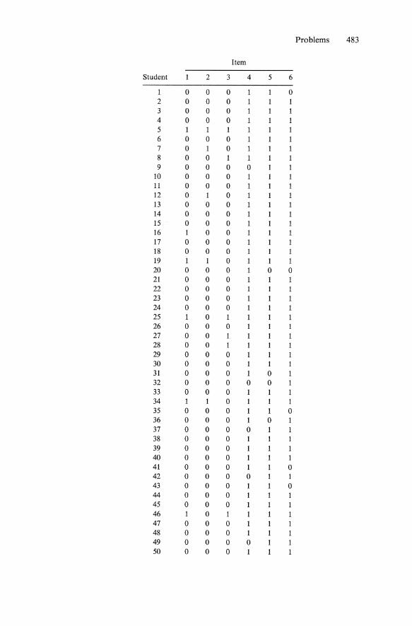
Problems 483
Item
Student 2 3 4 5 6
1 0 0 0 0 2 0 0 0 3 0 0 0 4 0 0 0 5 1 1 1 6 0 0 0 7 0 1 0 8 0 0 1 1 9 0 0 0 0
10 0 0 0 11 0 0 0 12 0 1 0 13 0 0 0 14 0 0 0 15 0 0 0 16 1 0 0 17 0 0 0 18 0 0 0 1 19 1 1 0 1 20 0 0 0 0 0 21 0 0 0 1 22 0 0 0 23 0 0 0 24 0 0 0 25 1 0 26 0 0 0 27 0 0 28 0 0 1 29 0 0 0 30 0 0 0 1 31 0 0 0 0 32 0 0 0 0 0 33 0 0 0 1 34 1 1 0 1 1 35 0 0 0 1 0 36 0 0 0 1 0 37 0 0 0 0 38 0 0 0 39 0 0 0 40 0 0 0 41 0 0 0 1 0 42 0 0 0 0 1 43 0 0 0 0 44 0 0 0 45 0 0 0 46 0 1 47 0 0 0 48 0 0 0 1 49 0 0 0 0 50 0 0 0

484 Problems
Item
Student 2 3 4 5 6
51 0 0 0 1 1 52 0 0 0 0 0 53 0 0 0 54 0 0 0 55 0 0 0 56 0 0 0 57 0 0 0 58 0 0 0 59 1 60 1 0 0 1 1 1 61 0 0 0 0 0 0 62 0 0 0 63 0 0 0 64 0 0 0 65 0 0 0 66 0 0 1 67 0 0 0 68 0 0 0 1 1 69 0 0 0 0 0 70 1 0 0 71 0 0 0 72 0 0 0 73 0 0 0 74 0 0 0 75 0 0 0 76 0 0 0 77 0 0 0 1 78 0 0 0 1 79 0 0 0 0 80 0 0 0 1 1 81 1 0 1 1 1 82 0 0 0 0 0 83 0 0 0 84 0 0 0 1 85 1 1 1 1 1 1 86 0 0 0 0 0 0 87 1 0 1 1 88 0 0 0 1 89 0 1 1 90 0 0 1 91 1 0 92 0 0 0 0 93 0 0 0 1 94 1 0 1 95 0 0 0 1 96 0 0 0 0 97 0 0 0 98 0 0 0 99 0 0 0 1 1 1
100 0 0 0 0 0 0

Problems 485
(Answer) The eigenvalues of the correlation matrix are 2.18, 1.41, .77, .75, .47 and .41. The factor pattern, following a varirnax rotation, is:
Factor
Item II h2
1 .861 .088 .749 2 .792 .077 .632 3 .665 .098 .452 4 .125 .624 .405 5 .057 .828 .688 6 .071 .813 .666
Consequently, the six items appear to form two factors. One factor is defined by items 1, 2, and 3, and the other factor is defined by items 4, 5, and 6. Note, however, that the item p values are .14, .12, .11, .89, .90, and .89, respectively. Therefore, the two factors simply reflect the fact that items 1, 2, and 3 are difficult and 4, 5, and 6 are easy. They are classical difficulty factors.

References
Applebaum, M.L, & Cramer, E.M. (1974). Some problems in the nonorthogonal analysis of variance. Psychological Bulletin, 81,335-343.
Atkinson, R.C. (1963). A variable sensitivity theory of signal detection. Psychological Review, 70,91-106.
Bartlett, M.S. (1937). The statistical conception of mental factors. British Journal of Psychology, 28,97-104.
Bartlett, M.S. (1950). Tests of significance in factor analysis. British Journal of Psychology, 3, 77-85.
Bentler, P.M. (1980). Multivariate analysis with latent variables: Causal modeling. Annual Review of Psychology, 31, 419-456.
Bentler, P.M. (1983). Some contributions to efficient statistics in structural models: Specification and estimation of moment structures. Psychometrika, 48, 493-517.
Bentler, P.M., & Bonnett, D.G. (1980). Significance tests and goodness of fit tests in the analysis of covariance structures. Psychological Bulletin, 88, 508-606.
Bernstein, I.H., & Eveland, D. (1982). State vs. trait anxiety: A case study in confirmatory factor analysis. Personality and Individual Differences, 3,361-372.
Bernstein, LH., Lin. T.-D., & McCleIIan, P. (1982). Cross- vs. within-racial judgments of attractiveness. Perception and Psychophysics, 32, 495-503.
Bernstein, I.H., & Garbin, C.P. (1985a). A comparison of alternative proposed sub scale structures for MMPI scale 2. Multivariate Behavior Research, 20, 223-235.
Bernstein, I.H., & Garbin, c.P. (1985b). A simple set of salient weights for the major dimensions of MMPI scale variation. Educational and Psychological Measurement, 45,771-787.
Bernstein, LH., Garbin, c.P., & McCleIIan, P.G. (1983). A confirmatory factoring of the California Psychological Inventory. Educational and Psychological Measurement, 43, 687-691.
Bernstein, I.H., Schoenfeld, L.S., & CosteIIo, R.L. (1982). Truncated component regression, multicoIIinearity and the MMPl's use in a police officer setting. Multivariate Behavior Research, 17, 99-116.
Bernstein, I.H., & Teng, G. (1986). Effects of item categorization and scale reliability upon factor structures. Unpublished manuscript.
Bernstein, I.H., Teng, G., & Garbin, C. P. (1986). A confirmatory factoring of the selfconsciousness scale. Multivariate Behaviorial Research, 21,459-475.
Blalock, H.M. (Ed.) (1971). Causal models in the social sciences. Chicago: Aldine. Boneau, C.A. (1960). The effects of violations of assumptions underlying the t test.
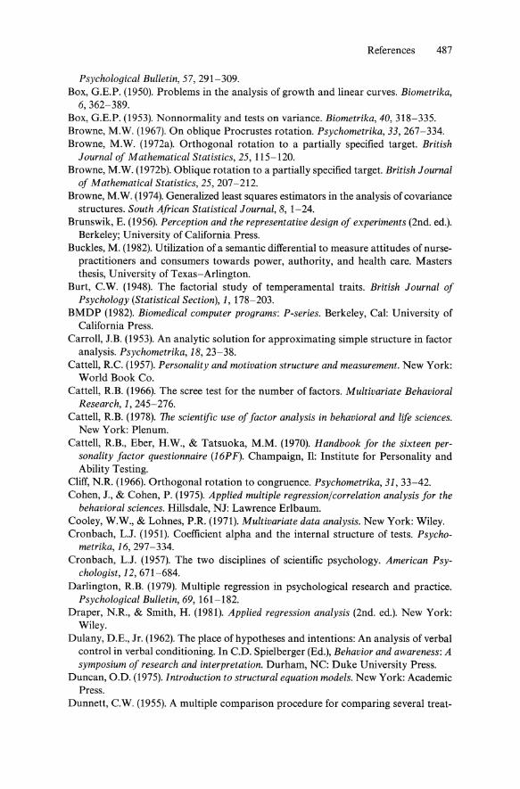
References 487
Psychological Bulletin, 57, 291-309. Box, G.E.P. (1950). Problems in the analysis of growth and linear curves. Biometrika,
6,362-389. Box, G.E.P. (1953). Nonnormality and tests on variance. Biometrika, 40,318-335. Browne, M.W. (1967). On oblique Procrustes rotation. Psychometrika, 33,267-334. Browne, M.W. (1972a). Orthogonal rotation to a partially specified target. British
lournal of Mathematical Statistics, 25, 115-120. Browne, M.W. (1972b). Oblique rotation to a partially specified target. British lournal
of Mathematical Statistics, 25, 207-212. Browne, M.W. (1974). Generalized least squares estimators in the analysis of covariance
structures. South African Statistical lournal, 8, 1-24. Brunswik, E. (1956). Perception and the representative design of experiments (2nd. ed.).
Berkeley; University of California Press. Buckles, M. (1982). Utilization of a semantic differential to measure attitudes of nurse
practitioners and consumers towards power, authority, and health care. Masters thesis, University of Texas-Arlington.
Burt, C.W. (1948). The factorial study of temperamental traits. British lournal of Psychology (Statistical Section), 1, 178-203.
BMDP (1982). Biomedical computer programs: P-series. Berkeley, Cal: University of California Press.
Carroll, J.B. (1953). An analytic solution for approximating simple structure in factor analysis. Psychometrika, 18, 23-38.
Cattell, R.c. (1957). Personaiity and motivation structure and measurement. New York: World Book Co.
Cattell, R.B. (1966). The scree test for the number of factors. Multivariate Behavioral Research, 1, 245-276.
Cattell, R.B. (1978). The scientific use of factor analysis in behavioral and life sciences. New York: Plenum.
Cattell, R.B., Eber, H.W., & Tatsuoka, M.M. (1970). Handbook for the sixteen personality factor questionnaire (16P F). Champaign, II: Institute for Personality and Ability Testing.
Cliff, N.R. (1966). Orthogonal rotation to congruence. Psychometrika, 31, 33-42. Cohen, J., & Cohen, P. (1975). Applied multiple regression/correlation analysis for the
behavioral sciences. Hillsdale, NJ: Lawrence Erlbaum. Cooley, W.W., & Lohnes, P.R. (1971). Multivariate data analysis. New York: Wiley. Cronbach, L.J. (1951). Coefficient alpha and the internal structure of tests. Psycho
metrika, 16, 297-334. Cronbach, L.J. (1957). The two disciplines of scientific psychology. American Psy
chologist, 12, 671-684. Darlington, R.B. (1979). Multiple regression in psychological research and practice.
Psychological Bulletin, 69, 161-182. Draper, N.R., & Smith, H. (1981). Applied regression analysis (2nd. ed.). New York:
Wiley. Dulany, D.E., Jr. (1962). The place of hypotheses and intentions: An analysis of verbal
control in verbal conditioning. In C.D. Spielberger (Ed.), Behavior and awareness: A symposium of research and interpretation. Durham, NC: Duke University Press.
Duncan, O.D. (1975). Introduction to structural equation models. New York: Academic Press.
Dunnett, C.W. (1955). A multiple comparison procedure for comparing several treat-

488 References
ments with a control. Journal oj the American Statistical Association, 50, 1096-1121. Dunnett, C.W. (1964). New tables for multiple comparisons with a control. Biometrics,
20,482-491. Egan, J.P. (1975). Signal detection theory and ROC analysis. New York: Academic
Press. Eriksen, C.M. (1960). Discrimination and learning without awareness: A method
ological survey and evaluation. Psychological Review, 67, 279-300. Feller, W.H. (1957). An introduction to probability theory and its applications (Vol I.,
2nd ed.). New York: Wiley. Ferguson, G.A. (1954). The concept of parsimony in factor analysis. Psychometrika,
19,281-290. Fisher, R.A. (1921). On the "probable error" of a coefficient of correlation. Metron, 1,
1-32. Fao, u.G. (1965). New developments in facet design and analysis. Psychological
Review, 72,262-274. Ford, L.S. (1981). Interspecific relationships among cloud forest frogs in the genus
Eleutherodactylus. Unpublished masters thesis, University of Texas-Arlington. Gaito, J, (1965). Unequal intervals and unequal n in trend analyses. Psychological
Bulletin, 63, 125-127. Garbin, c.P., & Bernstein, I.H. (1984). Visual and haptic perception of three-dimensional
solid forms. Perception and Psychophysics, 36, 104-110. Garner, W.R. (1960). Rating scales, discriminability, and information transmission.
Psychological Review, 67, 343-352. Garner, W.R. (1962). Uncertainty and structure as psychological concepts. New York:
Wiley. Garner, W.R., Hake, H.W., & Eriksen, C.W. (1957). Operationalism and the concept
of perception. Psychological Review, 63, 317-329. Gerbring, D.W. & Hunter, J. E. (1980). The return to multiple groups: Analysis and
critique of confirmatory factor analysis with LISREL. Unpublished manuscript. Gorsuch, R.L. (1966). The general factor in the Test Anxiety Questionnaire. Psy
chological Reports, 19, 308. Gorsuch, R.L. (1983). Factor analysis (2nd, ed.). Hillsdale, NJ: Lawrence Erlbaum. Green, D.M., & Swets, J.A. (1967). Signal detection theory and psychophysics. New
York: Wiley. Guilford, J.P. (1954). Psychometric methods (2nd. ed.). New York: McGraw-Hill. Guttman, L. (1952). Multiple group methods for common-factor analysis: Their basis,
computation, and interpretation. Psychometrika, 17, 209-222. Guttman, L. (1953). Image theory for the structure of quantitative variates. Psycho
metrika, 18, 277-296. Guttman, L. (1954). Some necessary conditions for common factor analysis. Psycho
metrika, 19, 149-161. Hake, H.W., & Rodwan, A.S. (1966). Perception and recognition. In J.B. Sidowski
(Ed.), Experimental methods and instrumentation in psychology. New York: McGrawHill.
Harman, H.H., & Jones, W.H. (1966). Factor analysis by minimizing residuals. Psychometrika, 31,351-368.
Harman, H.H. (1976). Modern Jactor analysis (3rd. ed., rev.). Chicago: University of Chicago Press.
Hays, W.L. (1981). Statistics (3rd ed.). New York: Holt, Rinehart, and Winston. Heck, D.L. (1960). Charts of some upper percentage points of the distribution of the

References 489
largest characteristic root. Annals of Mathematical Statistics, 31, 625-642. Heise, D.R. (1975). Causal Analysis. New York: Wiley. Hoaglin, D.e., Mosteller, F., & Tukey, J.W. (1983). Understanding robust and ex-
ploratory data analysis. New York: Wiley. Holzinger, K.J., & Swineford, F. (1937). The bi-factor method. Psychometrika, 2, 41-54. Holzinger, KJ. (1944). A simple method offactor analysis. Psychometrika, 9, 257-262. Hopkins, KD., & Stanley, J.e. (1981). Educational and psychological measurement and
evaluation (6th ed.). Englewood Cliff, NJ: Prentice-Hall. Horn, J.L. (1965). An empirical comparison of various methods for estimating common
factor scores. Educational and Psychological Measurements, 25, 313-322. Horst, P.W. (1963). Matrix algebra for social scientists. New York: Holt, Rinehart, and
Winston. Huberty, e.J. (1984). Issues in the use and interpretation of discriminant analysis.
Psychological Bulletin, 95, 156-171. Hulin, e.L., Drasgow, F., & Parsons, e.K (1983). Item response theory. Homewood,
IL: Dow Jones-Irwin. Hunter, J.E., & Schmidt, F.L. (1976). Critical analysis of the statistical and ethical im
plications of various definitions of Test Bias. Psychological Bulletin, 83,1053-1071. Hurley, J., & Cattell, R.B. (1962). The Pro.crustes program: Producing direct rotation
to test a hypothesized factor structure. Behavioral Science, 7,258-262. J6reskog, KG. (1967). Some contributions to maximum likelihood factor analysis.
Psychometrika, 32, 443-482. J6reskog, KG. (1969). A general approach to confirmatory maximum likelihood factor
analysis. Psychometrika, 34, 183-202. J6reskog, KG. (1974). Analyzing psychological data by structural analysis of covari
ance matrices, in R.e. Atkinson, D.H. Krantz, R.D. Luce, and P. Suppes (Eds.), Contemporary developments in mathematical psychology (Vol. II, pp. 1-64). San Francisco: Freeman.
J6reskog, KG., & S6rbom, D. (1986). LISREL: Analysis of linear structural relationships by the method of maximum likelihood (Version VI). Mooresville, IN: Scientific Software, Inc.
Kaiser, H.F. (1958). The varimax criterion for analytic rotation in factor analysis. Psychometrika, 23, 187-200.
Kaiser, H.F. (1960). The application of electronic computers to factor analysis. Educa-tional and Psychological Measurements, 20,141-151.
Kaiser, H.F. (1970). A second generation Little Jiffy. Psychometrika, 35, 401-417. Kaiser, H.F., & Caffey, J. (1965) Alpha factor analysis. Psychometrika, 30, 1-14. Kaiser, H.F., Hunka, S., & Bianchini, J. (1971). Relating factors between studies based
upon different individuals. Multivariate Behavioral Research, 6,409-422. Kemeny, J.G., Mirkil, H., Snell, J.N., & Thompson, G.L. (1959). Finite mathematical
structures. Englewood Cliffs, NJ: Prentice-Hall. Kenny, D.A. (1979). Correlation and causality. New York: Wiley. Keppel, G. (1982). Design and analysis: A researcher's handbook (2nd ed.). Englewood
Cliffs, NJ: Prentice-Hall. Kirk, R.E. (1968). Experimental design: Procedures for the behavioral sciences. Belmont,
CA: Brooks-Cole. Kmenta, J. (1971). Elements of econometrics. New York: Macmillan. Kruskal, J.B., & Wish, M. (1978). Multidimensional scaling. Beverly Hills, CA: Sage
Publications. Laughlin, J.E. (1978). Comment on "Estimating coefficients in linear models: It don't
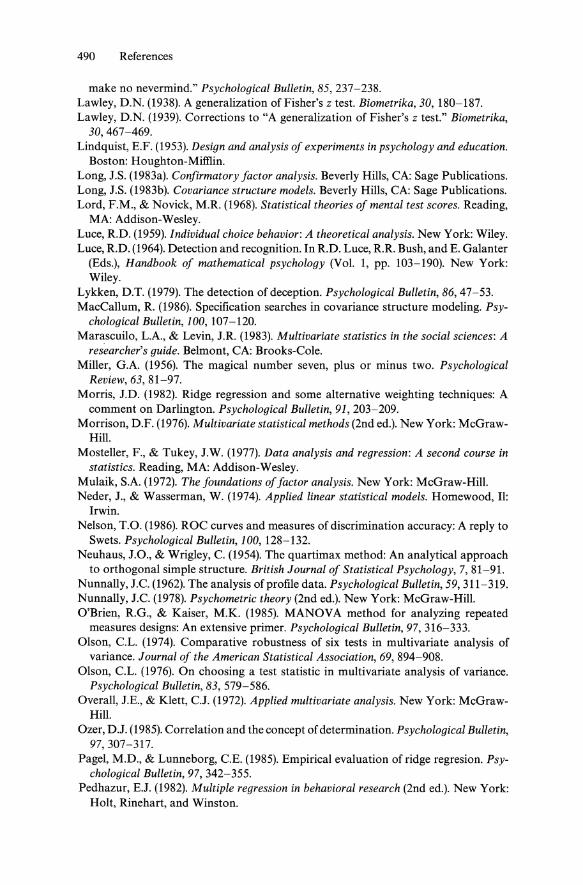
490 References
make no nevermind." Psychological Bulletin, 85, 237-238. Lawley, D.N. (1938). A generalization of Fisher's z test. Biometrika, 30, 180-187. Lawley, D.N. (1939). Corrections to "A generalization of Fisher's z test." Biometrika,
30,467-469. Lindquist, E.F. (1953). Design and analysis of experiments in psychology and education.
Boston: Houghton-Mifflin. Long, J.S. (1983a). Confirmatory factor analysis. Beverly Hills, CA: Sage Publications. Long, J.S. (1983b). Covariance structure models. Beverly Hills, CA: Sage Publications. Lord, F.M., & Novick, M.R. (1968). Statistical theories of mental test scores. Reading,
MA: Addison-Wesley. Luce, R.D. (1959). Individual choice behavior: A theoretical analysis. New York: Wiley. Luce, R.D. (1964). Detection and recognition. In R.D. Luce, R.R. Bush, and E. Galanter
(Eds.), Handbook of mathematical psychology (Vol. 1, pp. 103-190). New York: Wiley.
Lykken, D.T. (1979). The detection of deception. Psychological Bulletin, 86, 47-53. MacCallum, R. (1986). Specification searches in covariance structure modeling. Psy
chological Bulletin, 100, 107-120. Marascuilo, L.A., & Levin, J.R. (1983). Multivariate statistics in the social sciences: A
researcher's guide. Belmont, CA: Brooks-Cole. Miller, G.A. (1956). The magical number seven, plus or minus two. Psychological
Review, 63, 81-97. Morris, J.D. (1982). Ridge regression and some alternative weighting techniques: A
comment on Darlington. Psychological Bulletin, 91, 203-209. Morrison, D.F. (1976). Multivariate statistical methods (2nd ed.). New York: McGraw
Hill. Mosteller, F., & Tukey, J.W. (1977). Data analysis and regression: A second course in
statistics. Reading, MA: Addison-Wesley. Mulaik, S.A. (1972). The foundations of factor analysis. New York: McGraw-Hill. Neder, J., & Wasserman, W. (1974). Applied linear statistical models. Homewood, 11:
Irwin. Nelson, T.O. (1986). ROC curves and measures of discrimination accuracy: A reply to
Swets. Psychological Bulletin, 100, 128-132. Neuhaus, J.O., & Wrigley, C. (1954). The quartimax method: An analytical approach
to orthogonal simple structure. British Journal of Statistical Psychology, 7, 81-9l. Nunnally, J.C. (1962). The analysis of profile data. Psychological Bulletin, 59, 311-319. Nunnally, J.e. (1978). Psychometric theory (2nd ed.). New York: McGraw-Hili. O'Brien, R.G., & Kaiser, M.K. (1985). MANOVA method for analyzing repeated
measures designs: An extensive primer. Psychological Bulletin, 97, 316-333. Olson, e.L. (1974). Comparative robustness of six tests in multivariate analysis of
variance. Journal of the American Statistical Association, 69, 894-908. Olson, e.L. (1976). On choosing a test statistic in multivariate analysis of variance.
Psychological Bulletin, 83, 579-586. Overall, J.E., & Klett, e.J. (1972). Applied multivariate analysis. New York: McGraw
Hill. Ozer, D.J. (1985). Correlation and the concept of determination. Psychological Bulletin,
97,307-317. Pagel, M.D., & Lunneborg, e.E. (1985). Empirical evaluation of ridge regresion. Psy
chological Bulletin, 97, 342-355. Pedhazur, E.J. (1982). Multiple regression in behavioral research (2nd ed.). New York:
Holt, Rinehart, and Winston.
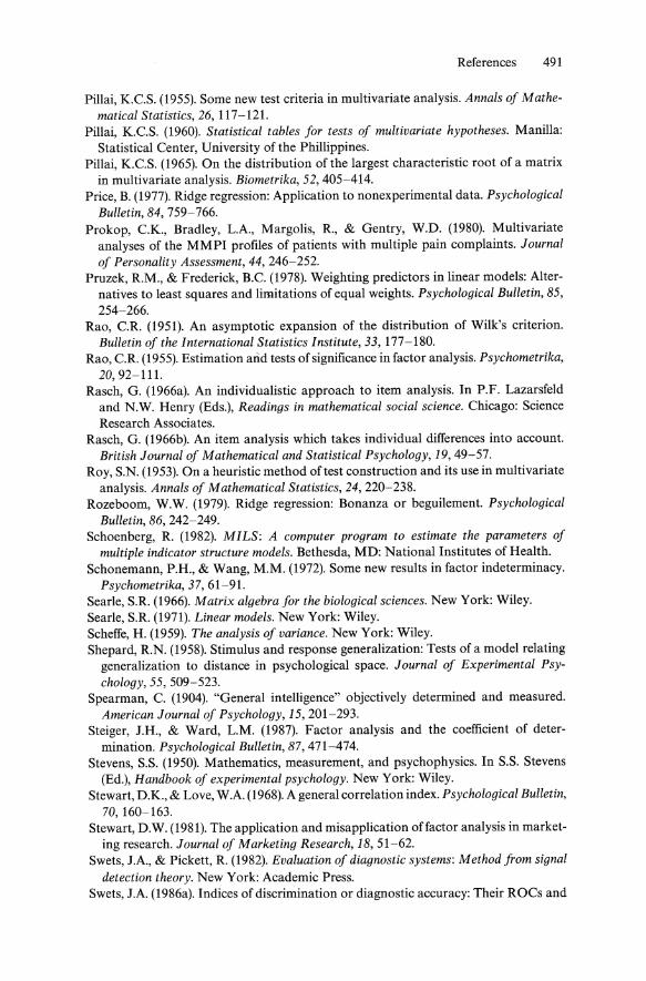
References 491
Pillai, K.C.S. (1955). Some new test criteria in multivariate analysis. Annals of Mathematical Statistics, 26,117-121.
Pillai, K.C.S. (1960). Statistical tables for tests of multivariate hypotheses. Manilla: Statistical Center, University ofthe Phillippines.
Pillai, K.C.S. (1965). On the distribution of the largest characteristic root of a matrix in multivariate analysis. Biometrika, 52, 405-414.
Price, B. (1977). Ridge regression: Application to nonexperimental data. Psychological Bulletin, 84, 759-766.
Prokop, c.K., Bradley, L.A., Margolis, R., & Gentry, W.D. (1980). Multivariate analyses of the MMPI profIles of patients with multiple pain complaints. Journal of Personality Assessment, 44, 246-252.
Pruzek, R.M., & Frederick, B.C. (1978). Weighting predictors in linear models: Alternatives to least squares and limitations of equal weights. Psychological Bulletin, 85, 254-266.
Rao, C.R. (1951). An asymptotic expansion of the distribution of Wilk's criterion. Bulletin of the International Statistics Institute, 33, 177-180.
Rao, c.R. (1955). Estimation arid tests of significance in factor analysis. Psychometrika, 20,92-P1.
Rasch, G. (1966a). An individualistic approach to item analysis. In P.F. Lazarsfeld and N.W. Henry (Eds.), Readings in mathematical social science. Chicago: Science Research Associates.
Rasch, G. (1966b). An item analysis which takes individual differences into account. British Journal of Mathematical and Statistical Psychology, 19,49-57.
Roy, S.N. (1953). On a heuristic method oftest construction and its use in multivariate analysis. Annals of Mathematical Statistics, 24, 220-238.
Rozeboom, W.W. (1979). Ridge regression: Bonanza or beguilement. Psychological Bulletin, 86, 242-249.
Schoenberg, R. (1982). MILS: A computer program to estimate the parameters of multiple indicator structure models. Bethesda, MD: National Institutes of Health.
Schonemann, P.H., & Wang, M.M. (1972). Some new results in factor indeterminacy. Psychometrika, 37, 61-9l.
Searle, S.R. (1966). Matrix algebra for the biological sciences. New York: Wiley. Searle, S.R. (1971). Linear models. New York: Wiley. Scheffe, H. (1959). The analysis of variance. New York: Wiley. Shepard, R.N. (1958). Stimulus and response generalization: Tests of a model relating
generalization to distance in psychological space. Journal of Experimental Psychology, 55, 509-523.
Spearman, C. (1904). "General intelligence" objectively determined and measured. American Journal of Psychology, 15, 201-293.
Steiger, J.H., & Ward, L.M. (1987). Factor analysis and the coefficient of determination. Psychological Bulletin, 87, 471-474.
Stevens, S.S. (1950). Mathematics, measurement, and psychophysics. In S.S. Stevens (Ed.), Handbook of experimental psychology. New York: Wiley.
Stewart, D.K., & Love, W.A. (1968). A general correlation index. Psychological Bulletin, 70, 160-163.
Stewart, D.W. (1981). The application and misapplication offactor analysis in marketing research. Journal of Marketing Research, 18, 51-62.
Swets, J.A., & Pickett, R. (1982). Evaluation of diagnostic systems: Method from signal detection theory. New York: Academic Press.
Swets, J.A. (1986a). Indices of discrimination or diagnostic accuracy: Their ROCs and
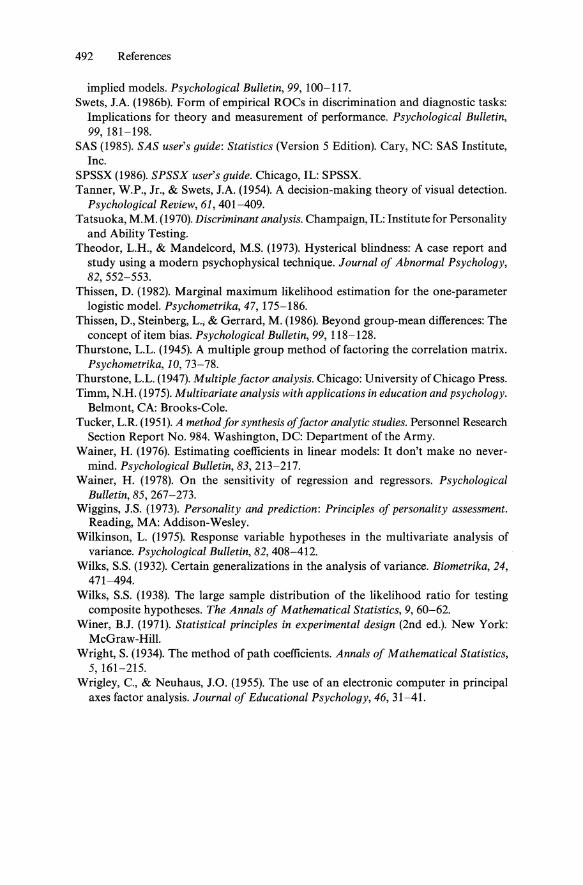
492 References
implied models. Psychological Bulletin, 99, 100-117. Swets, J.A. (1986b). Form of empirical ROCs in discrimination and diagnostic tasks:
Implications for theory and measurement of performance. Psychological Bulletin, 99,181-198.
SAS (1985). SAS user's guide: Statistics (Version 5 Edition). Cary, NC: SAS Institute, Inc.
SPSSX (1986). SPSSX user's guide. Chicago, IL: SPSSX. Tanner, W.P., Jr., & Swets, J.A. (1954). A decision-making theory of visual detection.
Psychological Review, 61, 401-409. Tatsuoka, M.M. (1970). Discriminant analysis. Champaign, IL: Institute for Personality
and Ability Testing. Theodor, L.H., & Mandelcord, M.S. (1973). Hysterical blindness: A case report and
study using a modern psychophysical technique. Journal of Abnormal Psychology, 82, 552-553.
Thissen, D. (1982). Marginal maximum likelihood estimation for the one-parameter logistic model. Psychometrika, 47, 175-186.
Thissen, D., Steinberg, L., & Gerrard, M. (1986). Beyond group-mean differences: The concept of item bias. Psychological Bulletin, 99, 118-128.
Thurstone, L.L. (1945). A multiple group method offactoring the correlation matrix. Psychometrika, 10, 73-78.
Thurstone, L.L. (1947). Multiple factor analysis. Chicago: University of Chicago Press. Timm, N.H. (1975). Multivariate analysis with applications in education and psychology.
Belmont, CA: Brooks-Cole. Tucker, L.R. (1951). A method for synthesis of factor analytic studies. Personnel Research
Section Report No. 984. Washington, DC: Department of the Army. Wainer, H. (1976). Estimating coefficients in linear models: It don't make no never
mind. Psychological Bulletin, 83, 213-217. Wainer, H. (1978). On the sensitivity of regression and regressors. Psychological
Bulletin, 85, 267-273. Wiggins, J.S. (1973). Personality and prediction: Principles of personality assessment.
Reading, MA: Addison-Wesley. Wilkinson, L. (1975). Response variable hypotheses in the multivariate analysis of
variance. Psychological Bulletin, 82, 408-412. Wilks, S.S. (1932). Certain generalizations in the analysis of variance. Biometrika, 24,
471-494. Wilks, S.S. (1938). The large sample distribution of the likelihood ratio for testing
composite hypotheses. The Annals of Mathematical Statistics, 9, 60-62. Winer, B.J. (1971). Statistical principles in experimental design (2nd ed.). New York:
McGraw-Hill. Wright, S. (1934). The method of path coefficients. Annals of Mathematical Statistics,
5, 161-215. Wrigley, c., & Neuhaus, J.O. (1955). The use of an electronic computer in principal
axes factor analysis. Journal of Educational Psychology, 46, 31-41.
Author Index
A Applebaum, M.l. 144,486 Atkinson, R.C. 285,486,489
B Bartlett, M.S. 174, 332, 486 Bentler, P.M. 189,201,222,486 Bernstein, l.H. 14, 42, 74, 113, 166,
187,208,211,273,399,400,405, 486, 488
Bianchini, J. 206, 489 Blalock, H.M. 228,486 Boneau, C.A. 331,486 Bonnett, D.G. 189,222,486 Box, G.E.P. 331,332,487 Bradley, L.A. 359,491 Browne, M.W. 189,208,219,487 Brunswik, E. 4,5,487 Buckles, M. 274,487 Burt, c.w. 208, 487
C Caffey, J. 160, 190,489 Carroll, J.B. 182, 487 Cattell, R.B. 165, 174, 208, 357, 399,
487,489 Cliff, N.R. 208, 487 Cohen, J. 120, 487 Cohen, ~ 120, 487 Cooley, w.w. 15, 112, 366, 487 Costello, R.L. 74, 113, 166,486
Cramer, E.M. 144, 486 Cronbach, L.J. 228,390,487
D Darlington, R.B. 113, 487 Draper, N.R. 112, 120, 487 Drasgow, F. 385,489 Dulany, D.E., Jr. 228, 487 Duncan,O.D. 228,487 Dunnett, C.w. 134, 487, 488
E Eber, H.w. 357,399,487 Egan, J.P. 291,275,279,488 Eriksen, C.w. 161,228,488 Eveland, D.C. 14,42,187,213,218,
400, 486
F Feller, W.H. 135, 488 Ferguson, G.A. 182, 488 Fisher, R.A. 42, 488 Foa, D.G. 326, 488 Ford, L.S. 274, 488 Frederick, B.C. 109, 491
G Gaito, J. 44, 138, 488 Garbin, c.P. 14,187,208,211,218,
273, 399, 486, 488

494 Author Index
Gamer, W.R. 160, 401, 488 Gentry, W.D. 359, 491 Gerbring, D.w. 224, 488 Gerrard, M. 385, 492 Gorsuch, R.L. 42,165,167, 183, 187,
194,201,203,224,488 Green, D.M. 275,279,283, 488 Guilford, 1.P. 381, 488 Guttman, L. 174,189,201,488
H Hake, H.w. 160, 275, 488 Harman, H.H. 76, 165, 183, 190, 194,
203,208,488 Hays, w.L. 30,31,45,127,135,429,
488 Heck, D.L. 328, 488 Heise, D.R. 228,489 Hoaglin, D.C 11, 489 Holzinger, K.1. 159,178,201,489 Hopkins, K.D. 381,489 Hom, I L. 193, 489 Horst, P.w. 59, 489 Huberty, C1. 275, 489 Hulin, CL. 385, 489 Hunka, S. 206,489 Hunter, 1.E. 103, 224, 488, 489 Hurley, 1. 208, 489
J Jones, W.H. 190, 488 J6reskog, K.G. 13, 162, 165, 189, 190,
201, 222, 489
K Kaiser, H.P. 83, 84, 109, 160, 174,
182, 183, 190,206,489 Kaiser, M.K. 326, 490 Kemeny, 1.G. 267, 489 Kenny, D.A. 228,489 Keppel, G. 127, 489 Kirk, R.E. 127, 489 Klett, C1. 15, 76, 256, 270, 313, 418,
423,490 Kmenta, 1. 222, 489
Krantz, D.H. 489 Kruskal, 1.B. 6, 489
L Laughlin, IE. 109,489 Lawley, D.N. 328, 490 Levin,IR. 43,331,363,490 Lin, T.-D. 212,218,486 Lindquist, E.E 331, 490 Lohnes, P.R. 15, 366, 487 Long, 1.S. 43, 201, 222, 490 Lord, EM. 385, 490 Love, W.A. 366, 491 Luce, R.D. 290,291,489,490 Lunneborg, CE. 113,490 Lykken, D.T. 290, 490
M MacCallum, R. 238, 490 Mandlecord, M.S. 288, 492 Marascuilo, L.A. 43,331,363,490 Margolis, R. 359, 491 McClellan, P.G. 212,218,486 Miller, G.A. 401,490 Mirkil, H. 267, 489 Morris, 1.D. 113, 490 Morrison, D.E 15, 329, 332, 490 Mosteller, E 11, 489, 490 Mulaik, S.A. 165, 194,490
N Neder, 1. 106, 490 Nelson, T.o. 294, 490 Neuhaus, J.0. 182,208,490, 492 Novick, M.R. 385,490 Nunnally,1.C 49,157,172,187,201,
356, 381, 490
o O'Brien, R.G. 326, 490 Olson, CL. 327, 490 Overall,1.E. 15, 76, 256, 270, 313,
418,423,490 Ozer, D.J. 48,490

p
Pagel, M.D. 113, 490 Parsons, e.K. 385, 489 Pedhazur, E.l 15, 112, 120, 123,228,
490 Pickett, R. 291, 491 Pillai, K.e.S. 328, 329, 331, 491 Price, B. 113, 491 Prokop, C.K. 359, 491 Pruzek, R.M. 109, 491
R Rao, e.R. 189, 330, 369, 491 Rasch, G. 385, 491 Rodwan, A.S. 275,488 Roy, S.N. 328, 491 Rozeboom, w.w. 113,491
S Scheffe, H. 127, 134, 491 Schmidt, F.L. 105, 489 Schoenberg, R. 190, 201, 222, 491 Schoenfeld, L.S. 74, 113, 166, 486 Schonemann, P.H. 187,491 Searle, S.R. 59, 491 Shepard, R.N. 290,491 Smith, H. 112, 120, 487 Snell, IN. 267,489 Sorbom, D. 13, 162, 165, 190,201,
222,489 Spearman, C. 177,491 Stanley, le. 381, 489 Steiger, lH. 48, 491
Author Index 495
Steinberg, L. 385, 492 Stevens, S.S. 37,491 Stewart, D.W. 366,491 Suppes, P. 489 Swets,lA. 275,279,283,291,294,
488,491,492 Swineford, F. 159, 178,489
T Tanner, w.P., Jr. 275,492 Tatsuoka, M.M. 357,399,487,492 Teng, G. 218, 399, 405, 486 Theodor, L.H. 288,492 Thissen, D. 385, 492 Thompson, G.L. 267,489 Thurstone, L.L. 159, 165, 178, 185,
201,492 Tirnm, N.H. 15,321,332,492 Tucker, L.R. 208,492 Tukey, lW. 11, 489, 490
W Wainer, H. 83, 84, 109,492 Wang, M.M. 187,491 Ward, L.M. 48, 491 Wasserman, W. 106, 490 Wiggins, lS. 326, 492 Wilkinson, L. 101,492 Wilks, S.S. 109, 328, 492 Winer, B.l 127, 134, 154, 492 Wish, M. 6, 489 Wright, S. 228,231,492 Wrigley, C. 182,208,490,492
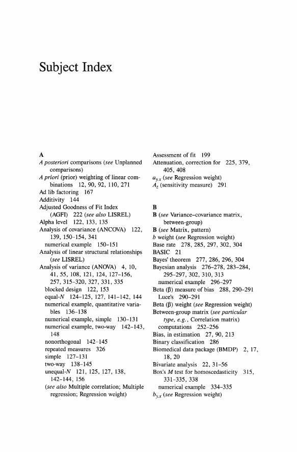
Subject Index
A A posteriori comparisons (see Unplanned
comparisons) A priori (prior) weighting of linear com-
binations 12, 90, 92, 110, 271 Ad lib factoring 167 Additivity 144 Adjusted Goodness of Fit Index
(AGFI) 222 (see also LISREL) Alpha level 122, 133, 135 Analysis of covariance (ANCOVA) 122,
139, 150-154, 341 numerical example 150-151
Analysis of linear structural relationships (see LISREL)
Analysis of variance (ANOVA) 4, 10, 41,55, 108, 121, 124, 127-156, 257,315-320,327,331,335
blocked design 122, 153 equal-N 124-125,127,141-142,144 numerical example, quantitative varia-
bles 136-138 numerical example, simple 130-131 numerical example, two-way 142-143,
148 nonorthogonal 142-145 repeated measures 326 simple 127-131 two-way 138-145 unequal-N 121,125,127, 138,
142-144, 156 (see also Multiple correlation; Multiple
regression; Regression weight)
Assessment of fit 199 Attenuation, correction for 225, 379,
405,408 ay.x (see Regression weight) Az (sensitivity measure) 291
B B (see Variance-covariance matrix,
between-group) B (see Matrix, pattern) b weight (see Regression weight) Base rate 278,285,297, 302, 304 BASIC 21 Bayes'theorem 277,286,296, 304 Bayesian analysis 276-278, 283-284,
295-297, 302, 310, 313 numerical example 296-297
Beta (/3) measure of bias 288, 290-291 Luce's 290-291
Beta (/3) weight (see Regression weight) Between-group matrix (see particular
type, e.g., Correlation matrix) computations 252-256
Bias, in estimation 27,90,213 Binary classification 286 Biomedical data package (BMDP) 2, 17,
18,20 Bivariate analysis 22,31-56 Box's M test for homoscedasticity 315,
331-335,338 numerical example 334-335
by.x (see Regression weight)
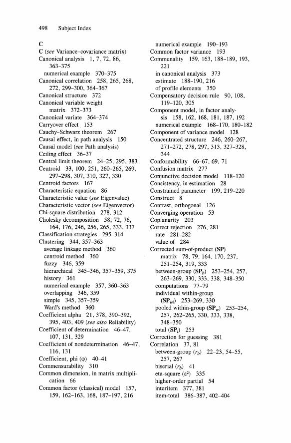
498 Subject Index
C C (see Variance-covariance matrix) Canonical analysis 1, 7, 72, 86,
363-375 numerical example 370-375
Canonical correlation 258, 265, 268, 272, 299-300, 364-367
Canonical structure 372 Canonical variable weight
matrix 372-373 Canonical variate 364-374 Carryover effect. 153 Cauchy-Schwarz theorem 267 Causal effect, in path analysis 150 Causal model (see Path analysis) Ceiling effect 36-37 Central limit theorem 24-25,295,383 Centroid 33, 100,251,260-265,269,
297-298, 307, 310, 327, 330 Centroid factors 167 Characteristic equation 86 Characteristic value (see Eigenvalue) Characteristic vector (see Eigenvector) Chi-square distribution 278, 312 Cholesky decomposition 58, 72, 76,
164, 176, 246, 256, 265, 333, 337 Classification strategies 295-314 Clustering 344, 357-363
average linkage method 360 centroid method 360 fuzzy 346, 359 hierarchical 345-346, 357-359, 375 history 361 numerical example 357, 360-363 overlapping 346, 359 simple 345, 357-359 Ward's method 360
Coefficient alpha 21,378, 390-392, 395, 403, 409 (see also Reliability)
Coefficient of determination 46-47, 107, 131,329
Coefficient of nondetermination 46-47, 116,131
Coefficient, phi (<p) 40-41 Commensurability 310 Common dimension, in matrix multipli
cation 66 Common factor (classical) model 157,
159,162-163,168,187-197,216
numerical example 190-193 Common factor variance 193 Communality 159,163,188-189, 193,
221 in canonical analysis 373 estimate 188-190,216 of profile elements 350
Compensatory decision rule 90, 108, 119-120,305
Component model, in factor analy-sis 158,162,168,181, 187, 192
numerical example 168-170, 180-182 Component of variance model 128 Concentrated structure 246, 260-267,
271-272,278,297,313,327-328, 344
Confonnability 66-67, 69, 71 Confusion matrix 277 Conjunctive decision model 118-120 Consistency, in estimation 28 Constrained parameter 199,219-220 Construct 8 Contrast, orthogonal 126 Converging operation 53 Coplanarity 203 Correct rejection 276, 281
rate 281-282 value of 284
Corrected sum-of-product (SP) matrix 78,79,164,170,237, 251-254,319,333
between-group (SPb) 253-254,257, 263-269, 330, 333, 338, 348-350
computations 77-79 individual within-group
(SPwi) 253-269,330 pooled within-group (SP w) 253-254,
257,262-265,330, 333, 338, 348-350
total (SPt) 253 Correction for guessing 381 Correlation 37, 81
between-group (rb) 22-23, 54-55, 257,267
biserial (rb) 41 eta-square (t2) 335 higher-order partial 54 interitem 377,381 item-total 386-387,402-404

non-Pearson 22, 40 part (semipartial) 22, 49-52 partial 22-23, 49-52 Pearson product-moment (r) 8, 22,
38-43,45,71, 172 point biserial (rpb) 40-41,248,317,
402 sampling error of 22, 42, 102 second-order partial 54 simple 117 Spearman (p, rank-order) 40 tetrachoric 41 total (rt) 21-23,54-55,267 within-group (r w) 21-23, 54-55, 267,
271 zero-order (simple) 50,53,97, 102 (see also Multiple correlation)
Correlation matrix (R) 57,61-62, 68-69, 79, 86, 88, 93, 95, 115, 126, 128, 164, 170, 174, 237, 257
between-group 254-255,259,264 computations 77 - 79 with desired factor structure (pro-
gram) 195-197 residual correlation 173, 175,215 total 254, 264 within-group 246,251,254,256,
264, 275, 354 Covariance 33,38-39,50,81,150
equation, in factor analysis 162, 236 Covariance matrix (see Variance-covari-
ance matrix) Covariate 50, 122, 150, 156 Criterion 7, 9, 89, 91 Cross validation 90, 109
double 110 CROSSTALK 15 Cubic clustering criterion 362 Cutoff 9, 285-286, 303 Cutoff rule 280 (see also Signal detec
tion theory)
D D (see Matrix, diagonal; Matrix, scaling) d (see Mahalanobis distance (d» d' (accuracy) measure 288-289,291,
293,295 Data transformation 30
Subject Index 499
Decision axis 9, 250, 276, 292-295 (see also Discriminant analysis; Signal detection theory)
Decision rule 280, 283 (see also Signal detection theory)
Decision variable, proper 292 Degrees of freedom (dj) 27, 107, 130 Dependent variable 4 Determinant 72-75, 87, 273
natural logarithm of 299 Difficulty factor 184, 398-399 Difficulty level 386 Diffuse structure 246,261-262,
267-272, 297-300, 313, 327-329, 344 (see also Factor analysis; Discriminant analysis)
Dimensional analysis 158, 166 Dimensionality, and item-level factor
ing 397 Direct effect, in path analysis 200,
234-235 Discriminant analysis 1,7,55,72,86,
117,246-344 numerical example with multiple
groups 263-271 numerical example with two
groups 252-256 Stepwise 246, 275 (see also Multivariate analysis of vari
ance (MANOVA» Discriminant axis 247, 259, 262,
266-270, 307-309, 336 Discriminant function 246-247,
250-251, 255-269, 301, 305, 307, 309, 312, 315, 330
Discriminant score 251,258,262,266, 270, 305-306, 309, 312
Discriminant structure 259, 299 Discriminant weight 246-257,268,301,
318,322,336 Discriminatory capacity 386, 387 Disjunctive decision rule 119-120 Distribution
asymmetric 26 binomial 29, 30 conditional 34 cumulative probability 31 frequency 23, 35 marginal 34

500 Subject Index
Distribution (cant.) parent 24-25 sampling 24-25 symmetric 26
Division, scalar 301 (see also Matrix "division"; Matrix inversion)
Domain sampling model 378, 387-389, 393-394
Dummy coding 121-123, 132-133, 140, 142, 145, 150
and plots of group means 153 (see also Multiple regression; Analysis
of variance) Dummy variable 129, 140
E E (see Eigenvector) Effect coding 121, 123-124, 133, 150
(see also Multiple regression; Analysis of variance)
Efficiency, in estimation 26, 28 Eigenanalysis 58, 85-88, 158, 170-173,
246,256-257,263-264,333,337, 360
numerical example 86-88, 173-174 Eigenvalue 58,85-87,170,173-175,
257,263-265,268,327-328,360, 367,403
Eigenvector 58,85-87,170-174,194, 256-257,268-269, 367
normalized 170 Elevation correction of profile 355-356 Ellipse 32 Endogenous variable, in path analy
sis 200,231-238 Envelope 32 Equal variance Gaussian model 276,
279-291 (see also Signal detection theory)
Equidiscriminating test construction 382, 400
Error variance 108, 187 Estimation 26-27, 92, 221
generalized least squares 221 least squares 28-29, 47, 93, 368 maximum likelihood 28-29, 43, 62,
221,224,286
minimum chi-square 28, 43 robust 11 unweighted least squares 221, 224
Eta (11), Luce's 290 Eta-square (112, correlation ratio) 41 Exogenous variable, in path analy-
sis 200,231-238 Exploratory analysis 11 (see also Factor
analysis, exploratory) Exponential distribution 293-295 Exponentiation 71
F F (see Matrix, factor score weight) F distribution 316 Fratio 10,131,133,137,143-144,
248,257,319,322,324, 327, 335, 340, 343
partial 257 F test 10, 106-107, 320, 328 Factor
bipolar 159, 177, 179,397 definition, as linear combina-
tion 79-80 general 159,176-179,183 graphic representation 180-182 group 159,176,179 oblique 186-187 orthogonal 178 singlet 159, 176 unipolar 159, 176 unique 157,162,176 varimax 405
Factor analysis 1, 7, 58, 81, 88 alpha method 159-160, 190 centroid method 175,211,213 confirmatory 11, 157, 164, 165,
188-246, 275, 398-399 diagonal method 175 exploratory 156-187,359,405 exploratory maximum likelihood
method 189 image method 189 item-level 378, 401 minimum residual method
(MINRES) 190

numerical example of common factor solution 190-193
numerical example of component solution 168-171
numerical example of LISREL 223-225
numerical example of oblique multiple groups 209-218
oblique multiple group computer program 239-245
oblique multiple group method (OMG) 165,198,201,209-225, 239, 275, 404, 406
orthogonal 368 pivotal condensation 175 principal components 168-172 raw-score 356 solid staircase method 175 square root method 175 (see also Matrix)
Factor definition 176-188 Factor equation 157, 161 Factor indeterminancy, first form 158,
163, 168 Factor indeterminancy, second
form 160, 192 Factor loading 177 Factor reliability 396 Factor rotation 176 Factor score 158-161, 166, 193-195,
202, 204-205 Factor structure 202 False alarm 276, 281, 284, 290 False alarm rate 281-283, 286-289, 294 Fisher classification function 310,
312-313 Fitting function 199,221 Fitting parallel lines 145 Fixed effect, in the analysis of vari
ance 122, 127, 155 Fixed parameter (constant) 199, 219,
220 Floor effect 37 Follower 219 FORTRAN 15, 21 Forward selection, in mUltiple regres
sion 111 Free parameter 199,219-220
Subject Index 501
G Gamma function (y) 308 Gaussian distribution, unequal vari
ance 294 (see also Signal detection theory)
General distance measure 94 Generalized inverse 68, 75 Generalized least squares 189 Goodness of Fit Index (GFl) 222, 224 Group centroid 311 Group effect, in the analysis of vari
ance 129 Guttman scale 386
H H (see Matrix, hypothesis) h2 (see Communality) Heteroscedasticity 34, 36-37, 106,
272-273,277-278,297, 303-304, 307, 320, 328
Heywood case 216 Hierarchical (Type I) model, in the analy
sis of variance 145 Hit 281-289,294
value of 284 Homoscedasticity 34, 37, 91, 273,
277-278, 297 Hotelling-Lawley trace (T) 315, 329,
334, 343-344 in canonical analysis 369
Hotelling's P 315,316,320-327,332 numerical example 323-324
Hypothesis testing 246
I I (see Matrix, identity) Identification, in LISREL 199,222 Incremental effect 108 Independent variable 3 Indicator, in LISREL 237 Indirect effect, in path analysis 200,
234-235 Inference 9 Interaction 122, 144 Interaction code 141 Interval variable 137

502 Subject Index
Introversion-extraversion 179 Invariance 206,213 Invariant value (see Eigenvalue) Invariant vector (see Eigenvector) Inversion, square-root method 76 "It don't make no nevermind" princi-
ple 83-84, 272, 303 Item 13
analysis 210, 386, 392 analysis, numerical example 400-406 difficulty 377 discrimination 377 distribution 382-383 homogeneity 388
Item response theory (IRT) model 385 Item trace (item operating characteris
tic) 377,381,383-387 Item~total correlation 377 Iteration 189
J Just-identified model, in LIS
REL 232-233
K Kaiser-Guttman ("A > 1")
criterion 174, 191
L A (see Eigenvalue) Latent variable 161 Latin square design 154 Law of parsimony 137 Leade~ inLISREL 219 Likelihood ratio 276-285, 292 Linear combination 7,33, 34, 58,
79-84, 95, 156, 165, 188, 198, 248, 258,271,294,346,351,364-365, 378
correlation between 82 covariances between 81 mean of 80 reliability of 395, 396 variance of 80
Linear dependency 73-75 Linear independence 58, 91
Linear model 139 Linear transformation 30, 31 Linearity of regression 91 LISREL 13, 18, 157, 159, 165, 190,
199-202,209-210,219-239,275, 399,405
Logistic distribution 290, 385
M Mahalanobis distance (d) 94, 258,
266-268,274,278,327,353-354 classification model 306-314
Main effect model, in the analysis of variance 145
Matched design 122, 153 Matrix
asymmetric 6 between-group 79 data 20, 57, 60 definition of 59 determinant of 58,329, 332, 350 deviation score 301 diagonal (D) 57,62,70,76, 173,367 discriminant weight 299 estimated correlation 219 factor correlation (<p) 83, 158,
163-164,215 factor score (F) 157, 160-161, 164 factor score weight (W) 212, 214, 364 gramian 58,72,85,88, 170 hypothesis (H) 214 identity (I) 57,63,68,74-75, 103,
158 ill-conditioned 58, 74, 350 inverse 58, 68, 69, 73, 76, 104 item intercorrelation 405 loading 171 lower triangular 63 nonsingular 58, 73 null 57,63,220,327 order 60,65 orthogonal 76, 158 orthonormal (transformation) 63-64,
68, 181 partitioned 69 pattern (B) 157,161-162,164,171,
208, 214, 215, 373 payoff 296

predictor intercorrelation (R) 194 pseudofactor hypothesis (Hp) 218 rank 50, 74, 75, 88, 178 scalar 62 scaling (D) 79, 83, 214 singular 58, 73, 75 singularity 73, 87 skew symmetric 62 square 57-61, 74, 86 structure (8) 159,171,203-204,214,
217 in Canonical analysis (8) 373 symmetric 6,57, 64, 70, 86, 265,
269 total 79 trace 57, 64, 87 transformation 208 transpose 68, 69, 72, 77, 88 triangular 57, 63, 72 uniqueness (U) 158, 163 upper triangular 63 within-group 79 z-score (Z) 57 (see also particular type, e.g., Correla-
tion matrix) Matrix addition 65 Matrix "division" 75 Matrix equality 57, 64 Matrix exponentiation 71-72 Matrix inversion 354 Matrix multiplication 57, 65-69
associative law 65, 67 commutative law 65, 67 distributive law 68
Matrix subtraction 65 Maximum expected value 285-286,
290 MDS (see Multidimensional scaling) Mean 23,38
adjusted group 151 geometric 39 trimmed 26 unadjusted group 151
Mean square 131 Measurement equation 236 Measurement model, in LIS-
REL 236-237 Measurement vector 270 Median 26
Subject Index 503
Mediating variable 235 MILS (see Multiple Indicator Linear
Structural Model) Minnesota Multiphasic Personality Inven
tory (MMPI) 17,29-32,77,83, 117-118,166,176,187,208, 272-273,277,298, 302, 348, 380-383, 400, 403, 407
depression (D) scale 387, 388 hysteria (Hy) scale 277-298, 301 psychopathic deviance (Pd)
scale 277-298, 301 lie (L) scale 391-392
Miss 276,281 value of 284
Miss rate 282 Model, substantive 217 Moderator effect 272 Modified Tucker-Lewis coeffi-
cient 222-226 Moment 38 Monotonicity 37 Multicollinearity 74, 83, 90, 92, 104,
113 Multidimensional scaling (MDS) 5 Multiple comparisons 108, 132, 213,
336, 346, 367 Multiple correlation (R) 7, 13, 88-156,
258 bias in 102
Multiple Indicator Linear Structural Model (MILS) 190,222,238
Multiple partialling 53 Multiple regression 1, 7, 15, 45, 59,
80,83,88-156,250,251,317,346, 368, 375
assumptions 91-93 geometry of 96 goals 93-96 hierarchical solution 12 inference in 106, 108 numerical example 114-118 simultaneous solution 12, 22, 93 stepwise solution 11-12,90,111-112
Multiplication, scalar 59 Multivariate analysis, broad defini
tion 1-6 Multivariate analysis, narrow defini
tion 1, 6-8

504 Subject Index
Multivariate analysis of covariance (MANCOVA) 1,7,316,341-344
numerical example 342-343 vs. repeated measures ANOVA 326
Multivariate analysis of variance (MANOVA) 1,7, 10,56,86, 315-344
multiple group 324-344 multivariate 316,336-340 numerical example 332-334, 338-341 post hoc comparisons 323 two group 316-326 (see also Discriminant analysis)
MS-DOS 17
N Nested effect, in the analysis of vari-
ance 149 Nested model, in LISREL 199,226 Nesting parameter, in LISREL 226 Noise (n) distribution 277, 279,
281-283,290 (see also Signal detection theory)
Noncausal effect, in path analysis 200, 235
Noncompensatory decision rule 90, 118, 120
Nonlinear (area) transformation 31 Nonmonotonicity 34 Nonnested model, in LISREL 199 Nonorthogonal comparisons, in the
analysis of variance 122, 133 Nonquantitative variable 121, 123 Nonrecursive model, in path analy
sis 200, 229, 235 Normal deviate 24 Normal distribution 23-25, 30-31, 41,
o
46,64,93, 306, 312 bivariate 22, 33, 46 multivariate 93, 329 standard normal 23
Oblique rotation 64 Oblique solution 164 Oblique transformation 64 (see also
Factor analysis)
Optimal weights 272 Order 75 Ordinal variable 137 Orthogonal coding 121, 123, 126, 133,
150 (see also Multiple regression; Analysis of variance)
Orthogonal comparisons 133-134 Orthogonal contrast 122 Orthogonal polynomial 136 (see also
Trend test) Orthogonal solution 164 (see also Factor
analysis) Orthogonality 82, 88, 142, 172, 184,
272 geometric 63, 269 statistical 269
Orthogonalization 158, 165 Orthonormal transformation 63 Outliers 10
p
Parallel form 201 Parallel test model 199, 227 Parameter 24, 26
constrained 221,225-226 fixed (constant) 221,225-226 free 225-226 locational 26
Partial derivative 223 PASCAL 21 Path analysis 122, 199-202, 227-237
numerical example 231-236 Path coefficient 199, 200, 228-323 Path diagram 229-233 Path regression coefficient 199, 228 Pattern bifactor 178 Pattern element 161, 177 Pattern probability model 313 Pattern weight 226 (jl (phi) (see Coefficient, phi) (f) (phi) (see Matrix, factor correlation) Pillai-Bartlett trace (V) 315,328,331,
334, 340, 343-344 in canonical analysis 369
Planned (a priori) comparisons 122, 133, 134
Platykurtosis 25 Polynomial function 122, 136
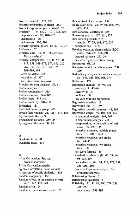
Positive manifold 172, 179 Posterior probability of signal 283 Postfactor (postmultiplier) 66-67, 70 Predictor 7,44,89,91, 101, 102, 108
importance of 90, 101-102 quantitative 96 uniqueness 102, 108
Prefactor (premultiplier) 66-67, 70, 77 Preference 62 Principal axes 34, 85, 188 (see also
Factor analysis) Principal components 33,44,58,90,
113, 158, 168-175, 179, 186,212, 269,346,360,369,374-375, 398-399, 403
cross-validated 406 reliability of 397 (see also Factor analysis)
Principal (major) diagonal 57,61 Profile analysis 1 Profile communality 353 Profile elevation 345-349 Profile shape 345-348 Profile similarity 346-356 Projection 181 Protected minority group 407 Pseudo-factor model 213,217,404,406 Psychometric theory 9 Pythagorean distance 259,267 Pythagorean theorem 94, 98
Q Quadratic form 81 Quadratic trend 136
R r (see Correlation, Pearson
product-moment) R (see Correlation matrix) rpb (see Correlation, point biserial) rs measure of profile similarity 356 Random assignment 150 Random effect, in the analysis of vari
ance 122, 127-128 Random error 24 Random error of measurement 155
Subject Index 505
Randomized block design 154 Range restriction 22, 39-40, 102, 398,
403,405 Raw canonical coefficient 255 Raw-score matrix 157, 161,237 Raw sum-of-products (SP)
matrix 77-79, 164, 170,237 computations 77-79
Receiver operating characteristic (ROC) curve 276-277, 286-291
unequal variance 293-294 (see also Signal detection theory)
Reciprocal 68, 75 Recursive model, in path analysis 200,
229 Redundancy analysis, in canonical analy
sis 346, 365-366, 368, 374 Reflection 177 Regression analysis 89, 94, 131
geometry of 43-44 linearity of 34 nonlinear 34 (see also Multiple regression)
Regression equation 13 Regression line 33, 159 Regression towards the mean 48, 394 Regression weight 95, 103, 124-125
in canonical analysis 364, 367 in discriminant analysis 256 interpretation, in the analysis of vari-
ance 124-129, 136 numerical example, multiple predic
tors 103-104, 114-118 numerical example, one predic-
tor 44-45 numerical example, two predic
tors 100 raw-score formula 45 standardized (beta or 13) 45, 59, 94,
98-103, 107 unstandardized (b) 94,115,177,251,
255, 258, 266 (see also Regression analysis; Dis-
criminant analysis) Relationship, linear 6 Relationship, quadratic 6 Reliability 21,30, 81, 190,379,381,
388-390 computations 391-393
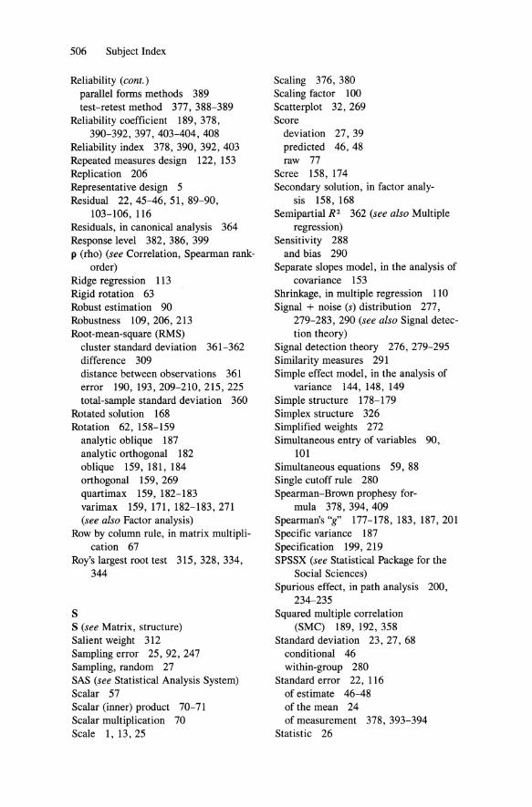
506 Subject Index
Reliability (cont.) parallel forms methods 389 test-retest method 377, 388-389
Reliability coefficient 189, 378, 390-392, 397, 403-404, 408
Reliability index 378, 390, 392, 403 Repeated measures design 122, 153 Replication 206 Representative design 5 Residual 22, 45-46, 51, 89-90,
103-106, 116 Residuals, in canonical analysis 364 Response level 382, 386, 399 P (rho) (see Correlation, Spearman rank-
order) Ridge regression 113 Rigid rotation 63 Robust estimation 90 Robustness 109, 206, 213 Root-mean-square (RMS)
cluster standard deviation 361-362 difference 309 distance between observations 361 error 190, 193,209-210,215,225 total-sample standard deviation 360
Rotated solution 168 Rotation 62, 158-159
analytic oblique 187 analytic orthogonal 182 oblique 159, 181, 184 orthogonal 159, 269 quartimax 159, 182-183 varimax 159, 171, 182-183, 271 (see also Factor analysis)
Row by column rule, in matrix mUltiplication 67
Roy's largest root test 315, 328,334, 344
s S (see Matrix, structure) Salient weight 312 Sampling error 25, 92, 247 Sampling, random 27 SAS (see Statistical Analysis System) Scalar 57 Scalar (inner) product 70-71 Scalar multiplication 70 Scale 1, 13, 25
Scaling 376, 380 Scaling factor 100 Scatterplot 32, 269 Score
deviation 27, 39 predicted 46, 48 raw 77
Scree 158, 174 Secondary solution, in factor analy
sis 158, 168 Semipartial R2 362 (see also Multiple
regression) Sensitivity 288
and bias 290 Separate slopes model, in the analysis of
covariance 153 Shrinkage, in multiple regression 110 Signal + noise (s) distribution 277,
279-283, 290 (see also Signal detection theory)
Signal detection theory 276, 279-295 Similarity measures 291 Simple effect model, in the analysis of
variance 144, 148, 149 Simple structure 178-179 Simplex structure 326 Simplified weights 272 Simultaneous entry of variables 90,
101 Simultaneous equations 59, 88 Single cutoff rule 280 Spearman-Brown prophesy for-
mula 378, 394, 409 Spearman's "g" 177-178, 183, 187,201 Specific variance 187 Specification 199, 219 SPSSX (see Statistical Package for the
Social Sciences) Spurious effect, in path analysis 200,
234-235 Squared multiple correlation
(SMC) 189, 192, 358 Standard deviation 23, 27, 68
conditional 46 within-group 280
Standard error 22, 116 of estimate 46-48 of the mean 24 of measurement 378, 393-394
Statistic 26

Statistical vs. experimental control 22, 53, 122, 153, 158, 167
Statistical Analysis System (SAS) 2, 17-21,194,251,255,321,328-332, 360-362, 392
PROC CANDISC 306 PROC CORR 20 PROC DISCRIM 306,312 PROC MANOVA 339 PROC MATRIX 20,21,239,390 PROC MATRIX, HALF opera-
tion 256 Statistical Package for the Social
Sciences (SPSSX) 2, 17-20, 168, 193, 195, 331, 392
PROC RELIABILITY 18,390 Strong substantive model 199-200,
225-227 Structural equation 236 Structural model, in LISREL 238 Structural program 200 Structure, between-group 266, 270 Structure element 177, 194,222 Structure, total 266, 270 Structure weight 186 Structure, within-group 266 Submatrix 58,69, 75 Successive entry of variables 90, 101,
III Sufficiency, in estimation 28 Sum of cross products measure 345,
355-356 Sum of squares 27
between-group 130 error 143 linear 136 quadratic 137 residual 137 total 130 within-group 130
Summation notation 69 Supermatrix 69 Suppressor variable 90, 98-99 Systematic design 5
T T (see Matrix, transformation) T (see Variance-covariance matrix, total)
t distribution 316 t ratio 248 t test 320, 324
Subject Index 507
Tau equivalent model 199, 201, 227 Temporal stability 377, 388 Test homogeneity (internal con-
sistency) 377 Test reliability 377 Third variable problem 9 Threshold effect 34, 36 Tolerance 104, 394 Total effect, in path analysis 235 Total matrix (see particular type, e.g.,
Correlation matrix) computations 252-256
Trace monotonicity 377 Transposition 64 Treatment effect, in the analysis of vari-
ance 155 Trend test 122, 136 Triangle, equilateral 268 Triangle, isosceles 268 Triangular matrix 256-257 Truncated component model 166 Two-alternative forced-choice task 291 Type I error 328, 335 Type II error 325 Type II model 145
U U (see Wilks' lambda) U (see Matrix, Uniqueness) Unadjusted model 145 Unanalyzed effect, in path analysis 200,
234,236 Uncorrected sum-of-products (SP) matrix
(see Raw sum-of-products (SP) matrix)
Unequal variance Gaussian model 277, 291-293
Uniform random number 60 Unit weight 271 Univariate analysis 22-31 Universal effect, in the analysis of vari-
ance 129 Unplanned comparisons 122, 133, 134 Unrotated solution 158 Unweighted mean 125

508 Subject Index
v V (see Pillai-Bartlett trace) Validity 4,98,101-103,117,317,366,
399,406 concurrent 406 construct 379, 407 content 379, 407 convergent 379,407 criterion 378 divergent 379, 407 face 408 postdictive 406 predictive 406-407
Variance 26-27, 39 accounted for 215 between-group 270 pooled within-group (within-
duster) 357-358 of profile elements 350 ofa sum 81 total 193 within-group 152, 270, 272
Variance-covariance matrix (C) 57,62, 74,78-79,88,350
between-group (B) 55, 254, 299 computations 77-79 group 333 individual within-group 298, 307,
311-313 pooled within-group (W) 251, 254,
267,273,298-299,307,311,313, 321, 323, 354
residual 81-82,158,162, 170, 173, 175,210,215,221,237,254,257
total (T) 55 within-group (see Variance-covariance
matrix, pooled within-group) Vector 60 Vector product 71
column 60, 64 "dot" (inner) 57, 66-67
matrix (outer) product 70 reference 185-186,215-216 row 60,64 unit 77
Vector (profile) similarity 347 Vectors, orthogonal 84
w W (see Hotelling-Lawley trace) W (see Variance-Covariance matrix,
pooled within-group) W (see Matrix, factor score weight) Weak substantive model 198-200,
219-220 Weighted mean 127 Wilks' lambda (U) 315, 328-329, 334,
343,344 Bartlett's chi-square test for 330, 339 in canonical analysis, Bartlett's proce
dure 369-370 in canonical analysis, Rao's proce
dure 369 Within-group matrix (see particular type,
e.g., Correlation matrix) computations 252-256
Within-subjects design 153
x X (see Raw-score matrix)
Y Yes-no task 291
z Z (see Matrix, z-score) 2' transformation 22, 42-43