Appendix A: A Dynamic Model of Retirement Decisions

The concept of the reduced-form participation elasticity can be motivated within adynamic framework that has been used extensively in the literature on retirement decisions.In particular, we refer to dynamic models by Stock andWise (1990) and Berkovec and Stern(1991), as well as on the reduced form models by Coile and Gruber (2007) and Gruber andWise (1999, 2004). In this framework a forward looking individual decides each periodwhether to continue working or to exit the labor market permanently and retire, based onan evaluation of the current and future bene�ts of continued work relative to the bene�tsof retirement. If tenure-based severance pay is introduced into this setting, the individualfaces a sharp increase in the incentive to retire once she reaches a tenure threshold, sincethe bene�ts from retiring have jumped to a higher level. Intuitively, our reduced-formelasticity measures the e¤ects on retirement decisions from the increase in the �nancialincentive at the tenure threshold.To formalize the role �nancial incentives on retirement decisions, we develop a simple

optimal stopping time model, which contrasts retirement decisions in a scenario withoutseverance pay to a scenario where individuals become eligible for severance pay once theyreach a tenure threshold.27 The model is designed to highlight the impacts of severance payand therefore, following the graphical evidence, we simplify the model by abstracting fromincentives to retire at certain ages. This simple model allows us to focus on two factors toexplain the patterns in the graphical evidence: (1) the changes in bene�ts at the tenurethresholds and (2) the option value from continuing to work (see Stock and Wise, 1990 fora similar option value model).We start with an employed individual at age 55 who decides whether to retire or continue

to work based on the discounted �ow of lifetime income under both options. Retirement isan irreversible decision, such that a retired individual does not have the choice to return towork and decisions are only possible as long as the individual stays employed. Considering�rst the scenario without severance pay, the decision in each period t, with t = 0 at age55, is based on a set of state variables:

t =

8>><>>:t agebt annual social security bene�ts if retiring at age ty annual earnings if working�t (disutility) costs of working at age t

The state variables evolve according to the following laws of motion. We assume that ageincreases by 1 each period and that earnings from employment y are �xed over time, whilethe level of bene�ts bt rises deterministically with each year of delay in retirement suchthat bt+1 > bt. The uncertainty in the model comes from �t, the cost of working, whichevolves according to a stochastic process with �t+1 = ��t + �t+1, where �t+1 � Ft(�t).27In the comparison of both scenarios we assume that severance pay only a¤ects the retirement decisions

of workers, but not any decisions at the employer�s side such as wage setting policy or hiring decisions.

1

At each age t the individual bases her decision on the set of value functions: The valuefor retirement is given by

V R(t; bt) = u(bt) + �tVR(t+ 1; bt);

and the value of employment is

V W (t) = u(y)� �t + �tEt[V (t+1)]:

We assume that consumption equals income in each period with per period utility given byu and there is no saving.28 The series of discount factors �t of future utility is assumed toalso capture the probability of survival. Et[V (t+1)] captures the expected value of nextperiod�s decision

V (t+1) = max�V R(t+ 1; bt+1); V

W (t+1):

The optimal strategy can be described by a reservation disutility value ��t(t), which deter-mines the retirement decision: the individual retires if �t � ��t(t). ��t is implicitly givenby the indi¤erence condition

V R(t; bt) = VW (t; bt; y; ��t)

Using a �rst order Taylor expansion of u around y, we can express the reservation disutilityas

��t = �(y � bt) + �tOVt (4)

where � denotes the marginal utility of consumption � = u0(y). This expression highlightsthe dependence of the reservation disutility on two components: the gain from workingy � bt in period t and the option value OVt of retiring at a later age which is given byOVt = Et[V

W (t+1)]�V R(t+1; bt) and incorporates future earnings and bene�ts as well asexpectations of future realizations of �t. Equation (4) de�nes ��t dynamically and in orderobtain a solution for ��t we solve the equation recursively starting at a �xed maximumlifetime T . For details see the next section. Let us call the gain from working ~yt and

28This is potentially a very crude approximation, as it also implies that individuals have to consumeseverance pay in a single period in the model scenario with severance pay. It does not a¤ect the mainmodel properties, however. Importantly, the option value always takes the potential receipt of futureseverance pay into account. We make this simplifying assumption for two reasons. First, we have no dataon consumption or savings and hence we cannot identify savings decisions. Second, this assumption allowsus to write net wages and implicit tax rates in terms of income di¤erences (i.e. earnings net of taxes andbene�ts) rather than consumption di¤erences. See the next footnote for more information.

2

re-write it in terms of the implicit tax rate � t de�ned as29

~yt = y(1� � t) = y � bt: (5)

Based on a solution for ��t we can express the hazard rate of retirement at age t as

ht = Prf�t > �yt(1� � t) + �tOVtg:

Given the hazard rates, the distribution of retirements by age nt is determined based onthe initial population size N0.In terms of policy tools we interpret the implicit tax rate � t as the key parameter

through which �nancial incentives can be manipulated by policy makers. Let us elaborateon this idea by introducing severance pay into the model. Severance pay enters the modelthrough the assumption that in addition to bt the individual receives a one time severancepayment amount of SP if she retires with a level of tenure higher than the thresholds�. Based on the empirical �ndings we make two simplifying assumptions. First, wemodel the severance pay policy with only one tenure threshold and second, we assume thattenure at age 55 is randomly assigned. This implies that the individual threshold dates areexogenous with respect to the other determinants of retirement and thresholds vary acrossthe population. To include severance pay into the retirement decision we include tenureTent as an additional state variable in SPt . Tenure increases by one in each period as longas an individual remains employed and it is set equal to zero at retirement. Under thisscenario the value functions change to

V R(t; bt) = u(bt + SP � I(Tent � s�)) + �tV R(t+ 1; bt)V W (SPt ) = u(y)� �t + �tEt[V (SPt+1)]

The equation for the reservation disutility ��SPt is given by

��SPt =

��(y � bt) + �tOV SPt if Tent < s�

�(y � bt � SP ) + �tOV SPt if Tent � s�(6)

For tenure levels above the threshold we de�ne the gain from working and the implicit tax

29In a more general model that allows for endogenous consumption decisions and hence consumptionsmoothing, the implicit tax rate could be de�ned in terms of consumption di¤erences,

(1� �)cWt = cWt � cRt

) � =cRtcWt:

In this expression, cWt denotes endogenous consumption if the individual were to choose to continue workingat time t and similarly cRt denotes endogenous consumption if the individual were to choose to retire attime t.

3

rate to include severance pay

~ySPt = y(1� �SPt ) = y � bt � SP: (7)

The corresponding hazard rate is given by

hSPt =

�Prf�t > �yt(1� � t) + �tOV SPt g if Tent < s�

Prf�t > �yt(1� �SPt ) + �tOV SPt g if Tent � s�:(8)

In this model scenario future decisions take the potential receipt of severance pay intoaccount and the option value of retirement at a later age OV SPt includes the option ofbecoming eligible for severance pay. Note that individuals receive severance pay if theyretire at any age after reaching the tenure threshold and the option value includes severancepay also at ages above the threshold. In other words, the option value of retiring at a laterage changes permanently at the tenure threshold, while severance pay changes the gainfrom working only in a single period.Equations (6) and (8) indicate that the option of severance pay will have di¤erent

e¤ects on the hazard rate depending on tenure. Prior to the tenure threshold severancepay increases the option value of delaying retirement and thus increases ��SPt and decreaseshSPt . After the threshold severance pay increases the implicit tax rate and increases thehazard rate. The equations for ��SPt and hSPt also indicate that induced by the jump in theimplicit tax rate at the tenure threshold, there will be a discrete drop in the reservationdisutility of work at the tenure threshold s� and a corresponding increase in the hazardrate. To investigate the shapes of the reservation disutility and hazard rates before andafter the tenure threshold in both scenarios with and without severance pay we turn tomodel simulations.

Model Simulations

To show the retirement decisions implied by our model over age and by tenure wesimulate model solutions for the two scenarios with and without severance pay. For speci�cdetails and assumptions of the model simulations are explained at the end of this section.We start with retirement outcomes for a cohort of identical individuals, who all have

the same level of tenure at age 55. We choose Ten0 = 2, which implies that they reach thetenure threshold s� at age 63. The following graphs trace the disutility of work and hazardrate into retirement for the cohort of individuals in both scenarios.Appendix Figure 4 plots the simulated pro�les of the reservation disutility of work ��t

and ��SPt by age. The downward sloping pro�le for the counterfactual scenario withoutseverance pay re�ects retirement decisions at older ages. Relative to the counterfactualwe see a sharp increase in the disutility of work prior to the threshold for individuals whobecome eligible for severance pay. Right after the threshold the reservation cost of workingdrops below the counterfactual and moves more or less parallel as individuals stay eligiblefor severance pay if they retire at any age after the threshold.

4

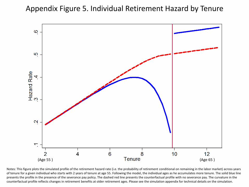
Appendix Figure 5 plots the corresponding simulated pro�les of the hazard rate intoretirement ht and hSPt by age. Not surprisingly the hazard rates re�ect the pro�le of thereservation disutility with higher disutilities implying lower hazards and vice versa.After having established the results at a single tenure/age threshold, we mix cohorts

of individuals with di¤erent levels of tenure at age 55 in the second set of simulations.Speci�cally we choose initial levels of tenure Ten0 = s0 with s0 ranging from 0 to 15 years.Individuals from the cohort with Ten0 = s0 have tenure s = t + s0 at age t and reach thetenure threshold s� = 10 at age t = 65� s0.For this group of individuals we focus on the average hazard rate to retirement by tenure

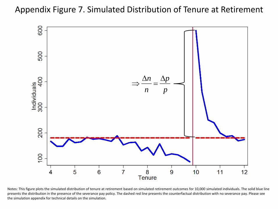
shown in Appendix Figure 6. This graph shows a constant average hazard of retirementin the counterfactual scenario, which results from averaging over di¤erent retirement ages.For the scenario with severance pay we see a dip in hazard rate prior to the tenure thresholdre�ecting the decline in the average hazards by age. We also see a large level shift in thehazard rate at the threshold and thereafter the hazard rate remains more or less constant.The next graph, Appendix Figure 7, relates the average hazard rate to the frequency of

retirements by the level of tenure. Given the initial cohort sizes we can compute retirementfrequencies by age and tenure nts and obtain the aggregate retirement frequency by tenurefrom ns =

PTt=0nts. This �gure represents the distribution of tenure at retirement or a

simulated equivalent of Figure 3. The simulated distribution of tenure is remarkably similarto the pattern observed in the data in Figure 3. In the simulated distribution the spike inretirement frequencies at the tenure threshold is a result from two factors: (i) the level shiftin the hazard rate and (ii) the fast decline in the population at risk of retiring after thetenure threshold. We further note that the in the simulated graph the frequency never goesto zero prior to the threshold, which is due to individuals retiring with very high values of��. In addition, the retirement frequency does not immediately drop to the counterfactuallevel in the period after the threshold, which re�ects the constantly high retirement hazardsas individuals stay eligible for severance pay if they retire in any period after the threshold.

Simulation Assumptions and Parameters

We assume that retirement decisions are made at a quarterly frequency from age 55through age 65 (i.e. everyone is assumed to be retired at age 66). For simplicity, weassume that there is no uncertainty due to mortality; all individuals live to age 85 withcertainty. The (quarterly) discount factor is � = 0:401=4. We specify the utility functionas u(c) = c1�

1� with = 0:5. Quarterly earnings are y =204. Quarterly retirement bene�ts

at age 55 are b55 = 124; for individuals retiring beyond age 55, retirement bene�ts increase

by 1% with each additional quarter of age beyond age 55. This increases in retirementbene�ts with retirement age continues up to a maximum level of retirement bene�ts equalto 0:99y. For the disutility of work �t, we set � = 0 and Ft as a uniform distribution over0 and �H ; to ensure that the disutility of work is on a similar scale as consumption (i.e.to avoid scenarios in which all individuals work or all individuals retire), the mean of thisuniform distribution is set to �t =

[0:04�y]1� 1� and �H = 2�t. Next, following the rules of

5

the Austrian severance pay system, we specify the severance payment amounts based ontenure and annual earnings. For expositional purposes, we scale the severance pay amountsby 0:25 (i.e. S ~P = 0:25 � SP ).To run the simulation, we specify the number of simulated individuals N0 = 10; 000.

For each individual, we draw initial tenure from a uniform distribution over [0,15]; weround tenure to the nearest quarter so that tenure is computed at a quarterly frequency.Given the parameter values and distributional assumptions above, we compute computethe individual�s value functions recursively and solve for the individual�s optimal retire-ment decision. In each period that the individual continues working, tenure and age bothincrease by 0:25 and the work disutility �t is randomly drawn from the uniform distrib-ution described above. Once the simulated individual retires, we record the individual�sretirement age, retirement tenure, work disutility (�t) and reservation disutility (��t) andthen continue to solve for the next simulated individual�s retirement outcome.

6

Appendix B: Retirement Age Elasticities

Conceptual Framework & De�ning the ElasticityThis section presents a static model of retirement decisions in the presence of a bud-

get constraints with notches from lump-sum severance payments. The model we use iscommon to both the public �nance literature and the retirement literature. In the public�nance literature, the model is a standard static labor supply model (for examples, see Saez2010 and Kleven and Waseem 2013); in the retirement literature, the model is a standardlifetime budget constraint model (see Brown 2013). We start by describing the model ofretirement decisions without severance payments and then introduce the payments. Themodel without severance payments can be interpreted as a model of counterfactual retire-ment decisions, i.e. what individuals�retirement decisions would be in the absence of anyseverance payment notches.We assume that each individual decides on labor supply over the life-cycle be choosing

his or her retirement age R. Following the public �nance literature on responses to incometax notches and kinks, we assume that the individual has quasi-linear preference overconsumption and labor supply. Consumption is based on total lifetime income from wagesw while working and pension bene�ts b while retired. We assume that the individual livesfor T periods and abstract from uncertainty and time discounting. Thus the individualchooses his retirement age by solving

maxRwR + (T �R)b� �

1 + 1e

�R

�

�1+ 1e

where the wR+ (T �R)b captures consumption based on lifetime income and �1+ 1

e

�R�

�1+ 1e

captures the disutility of labor supply. The parameter � is distributed across individuals inthe population according to density f(�) re�ecting that di¤erent individuals have di¤erenttastes for work and hence choose di¤erent retirement ages. The parameter 1

ecaptures

the curvature in the disutility of work or how quickly the marginal disutility from workrises if the individual increases his retirement age. Moreover, from the individual�s �rstorder condition, we can see that the parameter e captures the labor supply elasticity,e = d lnR

d ln(w�b) . This elasticity re�ects how much (as a percentage) an individual wouldincrease his retirement age by in response to a 1% increase in the net wage w � b.Next, we introduce lump-sum severance payments into the model; these payments create

upward notches the budget constraint. Speci�cally, we consider the case when individualsreceive a lump-sum payment SP if they retire at age R� or later.30 With the severance pay

30Here we focus on a single threshold and assume that the threshold occurs at the same age for allindividuals. We focus on a single threshold since this seems to be the most empirically relevant scenario asmost individuals retire between 55 and 60 and are likely to reach only 1 tenure threshold during this time.Since individuals reach age 55 with di¤erent years of tenure, individuals will face thresholds at di¤erentages. We discuss how we account for thresholds occurring at di¤erent ages in more detail below.

7

threshold, each individual�s optimization problem becomes

maxRwR + (T �R)b+ SP � 1(R > R�)� �

1 + 1e

�R

�

�1+ 1e

:

Appendix Figure 8 illustrates optimal retirement decisions comparing the smooth coun-terfactual budget constraint, with the budget set in the presence of the severance pay notch.If an individual would have chosen a retirement age above the threshold under the coun-terfactual (i.e. R > R�), her retirement decision is una¤ected by the additional incomefrom the severance payment. However, individuals who would have chosen a retirementage below the threshold might be induced by the severance pay to move to the thresholdretirement age R�. In particular, there is an individuals with taste �L who is indi¤erentindi¤erent between retiring earlier at RL < R� without the severance payment and retir-ing later at R� with the severance payment. All individuals who would have retired withR 2 (RL; R�) will be strictly better o¤ with the severance payment, so they all choose toretire at the threshold R�. The indi¤erence condition is given by

wR� + (T �R�)b+ SP � �L1 + 1

e

�R�

�L

�1+ 1e

| {z }utility from retiring at R� with severance pay

= w(RL) + (T �RL)b��L1 + 1

e

�RL�L

�1+ 1e

| {z }utility from retiring early at RL without severance pay

Given that labor supply is chosen optimally, the indi¤erent individual�s type is given by�L =

R���R�(w�b)e , where we denote by �R

� = R� � RL the length of delay. After substitutingthe expression for �L, the indi¤erence condition can be rewritten purely in terms of thethreshold R�, the length of delay �R�, the net wage w� b, the severance payment SP andthe labor supply elasticity e (see Kleven and Waseem 2012):�

1� �R�

R�

�+ e

�1� �R

�

R�

��1=e� (1 + e)

�1 +

SP

(w � b)R�

�= 0:

This expression makes clear that we can use the indi¤erence condition to recover thestructural labor supply elasticity e given that we have estimates for �R�

R� and SP(w�b)R� .

We can estimate the length of delay �R� from the retirement frequencies at the tenurethresholds, as we show below. The net wage w�b can be computed using average net wagefor individuals retiring near the threshold age. Similarly, the after-tax severance paymentSP can be computed by applying the severance payment rules and computing the averageafter-tax payment amount. The controversial parameter in the indi¤erence condition is thethreshold levelR�. It corresponds to the tenure threshold from the severance pay regulation,but in the model of life-cycle labor supply it translates to the retirement age at which theindividual reaches the tenure threshold. This ambiguity rises an important scaling issue.The scale of R� changes depending on the time horizon over which the individual makesher retirement decision, e.g. the full life cycle, the time since labor market entry, or the

8

time since age 55.From the form of the indi¤erence condition we can see that the estimated elasticity

is highly sensitive to the choice of scale of R�, with higher values of R� corresponding tosmaller elasticities.31 Relative to the sensitivity to the scaling parameter, the estimatedelasticity is not very sensitive to the severance pay fraction SP=(w � b), however. As theempirical estimation severance pay fraction is one of the main contributions of our paper,we discarded the elasticity concept based on the static labor supply model in the mainanalysis. In the empirical part of the elasticity computation in this Appendix section,we choose the main retirement age at which individuals reach the tenure thresholds asestimates for R� .The Length of Delay: Bunching and Adjustment CostsThe heterogeneity in tastes for work leads to a distribution of retirement age outcomes.

We denote the distribution of counterfactual retirement ages, i.e. the distribution in theabsence of the severance payments, by h0(R). Using this notation, and the result thatall individuals who have counterfactual retirement ages R� 2 [R� ��R�; R�] retire at thethreshold, the excess mass of individuals retiring at the threshold is

B =

Z R�

R���R�h0(r)dr �

�h0(R

�) + h0(R� ��R�)

2

�| {z }

h0

:

This equation for the excess mass (or bunching) implies that, given an estimate for B, thelength of delay can be estimated as �R� = B

h0.

One shortcoming of applying this strategy for estimating the length of delay is that themodel predicts holes in the distribution of labor supply outcomes with the notch. Speci�-cally, the model predicts that for e > 0, no individuals should choose labor supply outcomesbetween the point of indi¤erence and the threshold. Appendix Figure 9a illustrates thepredicted distribution of labor supply outcomes with a gap between the point of indi¤er-ence and the threshold. This prediction is at odds with what is observed in the data, sowe consider two alternative strategies to address this shortcoming.First, we assume that there is a �xed fraction of individuals who are constrained from

adjusting or choosing their retirement ages optimally (i.e. these individuals face involuntaryretirements and have exogenously given retirement ages). We denote this fraction by f . Inthis case, the length of delay can be estimated using �R� = B

(1�f)h0 ; the previous estimatefor �R� is now re-scaled by 1

1�f to account for the fact that a only fraction 1 � f canbunch at the threshold. As illustrated in Appendix Figure 9b, this predicts a �at numberof individuals �lling the pre-threshold gap in the distribution of of labor supply.Because this �rst strategy does not capture the downward-sloping pattern in the pre-

threshold distribution of labor supply, we also consider a second alternative strategy to cap-

31In our application a change of R� from 10 to 60 years roughly corresponds to an order of magnitudereduction in the estimated elasticity.

9

ture pre-threshold retirements. Speci�cally, we consider heterogeneous adjustment costs.32

We suppose that individuals each have an adjustment cost � distributed according to den-sity g(�) on [0; �max] with �max > 0 and � is independent from �. With the adjustmentcost, individuals adjust their retirement decision rules to retire at the threshold if and onlyif the utility from retiring at the threshold net of the adjustment cost exceeds the utilityfrom retiring earlier without the severance payment:

retire at R� i¤ usev � � > uno sev:

The cost � is therefore interpreted as a cost of adjusting from the counterfactual retirementage to the threshold age.With heterogeneous adjustment costs, at any given counterfactual retirement age, there

are some people with higher adjustment costs who do not move to the threshold andothers with lower adjustment costs who do move to the threshold. At or just above thepoint of indi¤erence, only individuals with 0 adjustment costs will choose to switch to thethreshold. For counterfactual retirements closer to the threshold, more individuals willchoose to switch. However, some individuals with counterfactual retirements just prior tothe threshold may still face su¢ ciently high adjustment cots so that they choose not toswitch. Thus, the model with heterogeneous adjustment costs does not predict a gap inthe distribution of labor supply outcomes and it predicts a downward-sloping pattern priorto the threshold. This prediction is illustrated in Appendix Figure 9c.In the presence of heterogeneous adjustment cots, the length of delay can be estimated

by estimating the point of indi¤erence since 0 adjustment costs apply at this point. Using anestimated distribution of counterfactual labor supply outcomes, the point of indi¤erencecan be estimated either by estimating the point at which the excess mass is completely�lled into the pre-threshold reduced mass or by estimating a point of convergence betweenthe observed and counterfactual distributions. As we discuss in more detail below, weimplement the second approach since it is more robust. We interpret the estimated elasticityfrom this strategy as an upper bound for the structural elasticity since the estimate is basedon determining the maximum length of delay.Estimating ProceduresThe retirement age elasticity can be estimated given an estimate for the length of delay

and values for the net wage, the severance payment, and the threshold retirement age.Since the other values can be directly observed or computed from the data, we focus onestimating the length of delay either using the amount of excess mass or using the pointof convergence. The estimation strategy �rst uses the distribution of tenure at retirement

32To account for pre-threshold retirements, we focus on heterogeneous adjustment costs with a homoge-neous elasticity rather than heterogeneous elasticities. We will investigate heterogeneity in elasticities inthe empirical analysis below by splitting the sample into di¤erent groups. However, we �nd heterogeneousadjustment costs to be a more plausible explanation for pre-threshold retirements than heterogeneouselasticities. To explain pre-threshold retirements with heterogeneous elasticities, a large fraction of thepopulation would need to have an elasticity of 0. It seems more intuitive that many people are constrainedfrom adjusting rather than being completely ignorant or never responsive.

10

to estimate a counterfactual distribution of tenure at retirement, and this counterfactualdistribution is then used to estimate the length of delay based on the two di¤erent strategies.The strategy then applies this estimated length of delay to multiple retirement ages toestimate elasticities at each retirement age, and �nally we compute a weighted average ofthe elasticities over all of the retirement ages.Identi�cation & Estimating CounterfactualsWith the retirement age elasticities, the identifying assumption and estimation of coun-

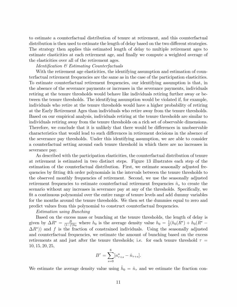
terfactual retirement frequencies are the same as in the case of the participation elasticities.To estimate counterfactual retirement frequencies, our identifying assumption is that, inthe absence of the severance payments or increases in the severance payments, individualsretiring at the tenure thresholds would behave like individuals retiring further away or be-tween the tenure thresholds. The identifying assumption would be violated if, for example,individuals who retire at the tenure thresholds would have a higher probability of retiringat the Early Retirement Ages than individuals who retire away from the tenure thresholds.Based on our empirical analysis, individuals retiring at the tenure thresholds are similar toindividuals retiring away from the tenure thresholds on a rich set of observable dimensions.Therefore, we conclude that it is unlikely that there would be di¤erences in unobservablecharacteristics that would lead to such di¤erences in retirement decisions in the absence ofthe severance pay thresholds. Under this identifying assumption, we are able to considera counterfactual setting around each tenure threshold in which there are no increases inseverance pay.As described with the participation elasticities, the counterfactual distribution of tenure

at retirement is estimated in two distinct steps. Figure 13 illustrates each step of theestimation of the counterfactual distribution. First, we estimate seasonally adjusted fre-quencies by �tting 4th order polynomials in the intervals between the tenure thresholds tothe observed monthly frequencies of retirement. Second, we use the seasonally adjustedretirement frequencies to estimate counterfactual retirement frequencies ns to create thescenario without any increases in severance pay at any of the thresholds. Speci�cally, we�t a continuous polynomial over the entire range of tenure levels and add dummy variablesfor the months around the tenure thresholds. We then set the dummies equal to zero andpredict values from this polynomial to construct counterfactual frequencies.Estimation using BunchingBased on the excess mass or bunching at the tenure thresholds, the length of delay is

given by �R� = B(1�f)h0 where h0 is the average density value h0 =

12(h0(R

�) + h0(R� �

�R�)) and f is the fraction of constrained individuals. Using the seasonally adjustedand counterfactual frequencies, we estimate the amount of bunching based on the excessretirements at and just after the tenure thresholds; i.e. for each tenure threshold � =10; 15; 20; 25,

B� =

6Xs=0

[na�+s � n�+s].

We estimate the average density value using h0 = n� and we estimate the fraction con-

11

strained using the fraction of individuals who retire one month prior to the tenure threshold,

f =na��1n��1

:

Thus, given each of these estimates, we are able to estimate the length of delay at eachtenure threshold based on the bunching at the threshold and the fraction constrained justbefore the threshold.Estimation using Point of ConvergenceWe also estimate the length of delay using the point of convergence between the actual

and counterfactual distributions of tenure at retirement. This point of convergence capturesthe point of indi¤erence between retiring earlier without the severance payment and retiringlater at the tenure threshold with the severance payment. Furthermore, at this point ofindi¤erence, no adjustment costs apply by assumption. We estimate the length of delaybased on the point of convergence for each threshold as the prior point closest to thethreshold such that the di¤erence between the actual and counterfactual frequencies is lessthan 5% of the counterfactual frequencies,

min s > 0 such thatna��s � n��s

n��s< 0:05:

Accounting for Thresholds at Di¤erent Retirement AgesWhile the counterfactual distribution is used to estimate a length of delay at each

tenure threshold, the elasticity estimation must still take into account that individualsreach the tenure thresholds at di¤erent retirement ages. We account for this fact by usingweights based on the fraction of people who retire at each age around each tenure threshold.Speci�cally, for each tenure threshold � = 10; 15; 20; 25, we identify all individuals whoretire with tenure t 2 [� � 2; � + 2]; we denote this group of individuals by N � . For eachof these groups of individuals, we compute the fraction of individuals who retire at eachage a = 55; :::; 65; we denote these fractions by p�a. For each retirement age a = 55; :::; 65,we compute the average net wage and severance payment amounts directly from the dataand we use the indi¤erence condition with the estimated length of delay at the tenurethreshold �R�� to estimate labor supply elasticities e

�a. Using the retirement age fractions,

we compute a weighted average of these elasticities,

e� =65Xa=55

p�ae�a:

This strategy yields an estimated elasticity for each tenure threshold. We also computea weighted average elasticity across the tenure thresholds using e =

P�

�N�

N

�e� where

N =P

� N�

Estimation ResultsTable C1 presents the estimation results at each tenure threshold for men and women

12

separately The �rst row presents the excess retirement frequencies within each tenurethreshold, B� for � = 10; 15; 20; 25. The second row presents estimates of the fractionof constrained individuals, f � , using the fraction of individuals retiring one month priorto a tenure threshold. The estimates across the tenure thresholds indicate that between63% and 80% of men could be constrained while between 43% and 61% of women could beconstrained. Using these fractions, the estimated length of delay is between 0.40 and 0.52years for men and between 0.40 and 0.66 years for women. The estimated lengths of delayare used to estimate lower bounds for the retirement age elasticity, and these estimatedretirement age elasticities are presented in the �fth row of Table C1. The estimated lowerbound elasticities are close to 0. These estimated elasticities are relatively small becausethe estimated length of delay is on the order of 6 months, and the model requires a smalllabor supply elasticity if individuals are only willing to delay their retirements by 6 monthsin the presence of signi�cant notches in their budget constraints from the severance pay-ments. Intuitively, the disutility of labor supply must rise very quickly with additional timeat work if individuals are only willing to delay their retirements by 6 months when thereare sizeable �nancial incentives from the severance payments.We also estimate upper bounds for the retirement age elasticity parameter using esti-

mates for the point of convergence prior to each tenure threshold. The estimated points ofconvergence are between roughly 0.66 and 1.42 years prior to a tenure threshold for men,and between 1.00 and 1.42 years for women. These estimates indicate that individuals arewilling to delay their retirements by longer periods of time then the estimated lengths ofdelay based on the excess retirements and fractions constrained implied. The estimatedupper bound retirement age elasticities based on these estimated points of convergence arereported in row 6 of Table C1. We estimate elasticities between 0.007 and 0.015 for menand between 0.007 and 0.044 for women. Taking weighted averages over all of the tenurethresholds yields estimated elasticities of 0.01 for men and 0.02 for women.These estimated retirement age elasticities are consistent with previous estimates in

the literature. In particular, using maximum likelihood and nonparametric estimationtechniques based on a kink in the budget constraint, Brown (2013) estimates retirementage elasticities on the order of 0.02 (see Tables 2 and 3 of Brown 2013). While Brown�sestimated apply to a sample of teachers in California, the elasticities reported in Table C1are based on a large sample of private sector employees throughout Austria. Overall, theestimated elasticities indicate relatively low responsiveness to �nancial incentives to delayretirement. The estimated elasticities also highlight signi�cant di¤erences between menand women.

13

Appendix C: Construction of Implicit Tax Rates

The social security data report gross annual earnings at the individual level for eachyear and employer. To compute implicit tax rates we need information on pension bene�tsplus wages and pensions net of social security contributions and income taxes.We use the following procedure to generate estimates of these additional variables:

First, we calculate the pension bene�t that the individual would receive if they retired inthe current year based on earnings and employment histories according to the legislation ofthe pension system. We start calculating pensions in the year when the individual turns 55up to the year of actual retirement. Second, we use information from tax records availablefor the years 1994-2005 to estimate the corresponding net wages and net pensions for oursample.33

The ASSD reports gross earnings after the employer�s share of social security contribu-tions has been paid. Then the employee�s share of social security contributions is deductedfrom the gross earnings and �nally income taxes are withheld. The employee�s contributionshare covers health insurance, pension insurance, unemployment insurance and contribu-tions to health insurance for retirees. The rates are constant across individuals and hardlychange over time. We use average social security contribution rates from the tax �les, whichare 17.5% for employees and 3.8% for retired workers. Taxes are based on gross earningsminus social security contributions. The tax schedule is progressive and is applied to thetax basis after individual deductions. Because these deductions vary by family composi-tion and other characteristics unobservable to us, we estimate separate average tax ratesfor women and men, employed and retired workers. Over time tax rates and brackets wererepeatedly adjusted to wage growth. We therefore divide the observable period into threedi¤erent tax regimes, which cover the most important tax reforms: before 1996, 1996-2000,after 2000.The sample used for estimating average tax rates consists of all earnings records of

wages and pensions of individuals born between 1930 and 1940 who are covered in the1994 - 2005 tax records. We restrict the observations to earnings below the contributioncap, because of censoring in the social security data. To limit the problem with multiplerecords per individual we only consider records for income that was received for the fullcalender year. For each tax regime we pick one representative year: 1994, 1999, 2003.Then we compute 20 percentiles in each of these years to get a representative distributionof gross wages and pensions. Next we categorize the earnings in each regime accordingto the percentile distribution and compute in each earnings cell the average tax rates formen, women, wages, and pensions by the average ratio of taxes to gross wages minus socialsecurity contributions. The median of average tax rates increases from the �rst to the thirdtax regime from about 11% to 13% for wage income and from 7% to 9% for pension income.In all groups taxes on female earnings are slightly above taxes for males. The maximumaverage tax rates reach 20%.

33For a description of the tax data see Section 2.3.

14

In the �nal step we apply the average tax rates to wage earnings and simulated pensionbene�ts for the individuals of our retirement sample and compute implicit tax rates as

(1� �)gross_earn = gross_earn� ss_contrib� inc_tax� pension+�SSW

) � =ss_contrib+ inc_tax+ pension��SSW

gross_earn:

15

Median Earner 0.5 0.75 1 1.5 2 Median Earner 0.5 0.75 1 1.5 2Australia 47.9 70.7 52.3 43.1 33.8 29.2 61.7 83.5 66.2 56.4 46.1 40.8Austria 80.1 80.1 80.1 80.1 78.5 58.8 90.6 90.4 90.6 90.9 89.2 66.4Belgium 40.7 57.3 40.9 40.4 31.3 23.5 64.4 77.3 65.5 63 51.1 40.7Canada 49.5 75.4 54.4 43.9 29.6 22.2 62.8 89.2 68.3 57.4 40 30.8Czech Republic 54.3 78.8 59 49.1 36.4 28.9 70.3 98.8 75.6 64.4 49.3 40.2Denmark 83.6 119.6 90.4 75.8 61.3 57.1 94.1 132.7 101.6 86.7 77 72.2Finland 63.4 71.3 63.4 63.4 63.4 63.4 68 77.4 68.4 68.8 70.3 70.5France 51.2 63.8 51.2 51.2 46.9 44.7 62.8 78.4 64.9 63.1 58 55.4Germany 39.9 39.9 39.9 39.9 39.9 30 57.3 53.4 56.6 58 59.2 44.4Greece 95.7 95.7 95.7 95.7 95.7 95.7 111.1 113.6 111.7 110.1 110.3 107Hungary 76.9 76.9 76.9 76.9 76.9 76.9 96.5 94.7 95.1 102.2 98.5 98.5Iceland 80.1 109.9 85.8 77.5 74.4 72.9 86.9 110.9 92 84.2 80.3 79.7Ireland 38.2 65 43.3 32.5 21.7 16.2 44.4 65.8 49.3 38.5 29.3 23.5Italy 67.9 67.9 67.9 67.9 67.9 67.9 77.9 81.8 78.2 77.9 78.1 79.3Japan 36.8 47.8 38.9 34.4 29.9 27.2 41.5 52.5 43.5 39.2 34.3 31.3Korea 72.7 99.9 77.9 66.8 55.8 45.1 77.8 106.1 83.1 71.8 61.9 50.7Luxembourg 90.3 99.8 92.1 88.3 84.5 82.5 98 107.6 99.8 96.2 92.9 91Mexico 36.6 52.8 37.3 35.8 34.4 33.6 37.9 50.3 37.8 38.3 39 40Netherlands 81.7 80.6 81.5 81.9 82.4 82.6 105.3 97 103.8 96.8 96.3 94.8New Zealand 46.8 79.5 53 39.7 26.5 19.9 48.6 81.4 54.9 41.7 29.4 23.2Norway 60 66.4 61.2 59.3 50.2 42.7 70 77.1 71.2 69.3 62.5 55.1Poland 61.2 61.2 61.2 61.2 61.2 61.2 74.8 74.5 74.8 74.9 75 77.1Portugal 54.3 70.4 54.5 54.1 53.4 52.7 67.4 81.6 66 69.2 72.2 73.7Slovak Republic 56.7 56.7 56.7 56.7 56.7 56.7 71.9 66.4 70.6 72.9 75.4 76.7Spain 81.2 81.2 81.2 81.2 81.2 67.1 84.2 82 83.9 84.5 85.2 72.4Sweden 63.7 79.1 66.6 62.1 64.7 66.3 66.2 81.4 69.2 64 71.9 73.9Switzerland 62 62.5 62.1 58.4 40.7 30.5 68.8 75 68.2 64.3 45.7 35.1Turkey 72.5 72.5 72.5 72.5 72.5 72.5 103.4 101 102.9 104 106.4 108.3UK 34.4 53.4 37.8 30.8 22.6 17 45.4 66.1 49.2 41.1 30.6 24US 43.6 55.2 45.8 41.2 36.5 32.1 55.3 67.4 58 52.4 47.9 43.2

OECD 60.8 73 62.7 58.7 53.7 49.2 72.1 83.8 74 70.1 65.4 60.7

Italy 52.8 52.8 52.8 52.8 52.8 52.8 63.8 63.6 64.4 63.4 63.7 63.5Mexico 31.1 52.8 35.2 29.7 28.5 27.9 32.2 50.3 35.7 31.7 32.3 33.2Poland 44.5 46.2 44.5 44.5 44.5 44.5 55.3 57.5 55.3 55.2 55 56.4Switzerland 62.6 62.8 62.6 59.1 41.2 30.9 68.1 75.4 68.9 65 46.3 35.5

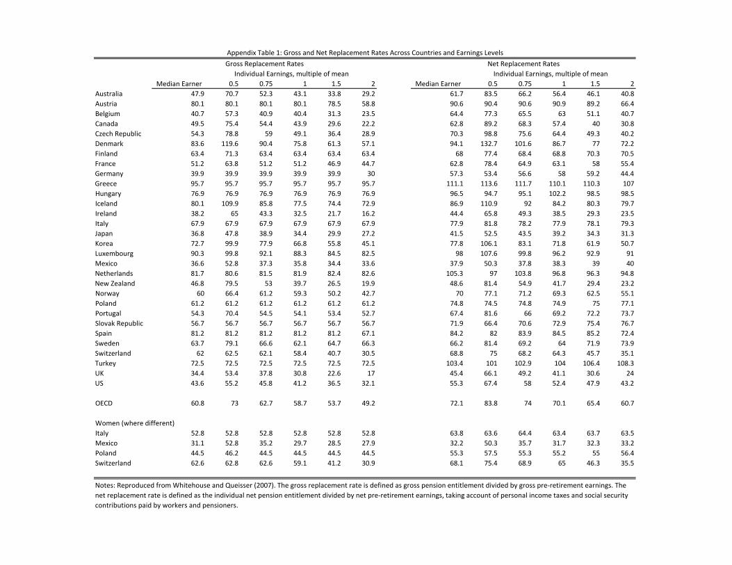
Notes: Reproduced from Whitehouse and Queisser (2007). The gross replacement rate is defined as gross pension entitlement divided by gross pre-retirement earnings. The net replacement rate is defined as the individual net pension entitlement divided by net pre-retirement earnings, taking account of personal income taxes and social security contributions paid by workers and pensioners.

Women (where different)

Gross Replacement RatesIndividual Earnings, multiple of mean

Appendix Table 1: Gross and Net Replacement Rates Across Countries and Earnings LevelsNet Replacement Rates

Individual Earnings, multiple of mean

Number of Individuals Percentage change

Individuals in cohorts born 1930 - 1945,still employed at age 54 with more than one year of work experience 700,590Excluding workers ever employed as civil servant 623,055 -11%Workers retiring withing 6 months of their last job 424,598 -32%Excluding workers with last job in construction 381,239 -10%Excluding left censored tenure in last job 293,824 -23%Individuals with 6 - 28 years of tenure 194,086 -34%Sample matched with tax data:Individuals retiring between 1997 and 2005 97,107 -50%Matched severance pay in tax data 89,426 -8%

Notes: Numbers based on the ASSD.

Appendix Table 2: Sample Selection

Coefficient Standard Error Coefficient Standard Error Coefficient Standard Error1(Female) 0.019 0.0061(Blue Collar) 0.015 0.005 -0.009 0.006 0.038 0.0071(Austrian Citizen) -0.041 0.010 -0.037 0.013 -0.034 0.0151(Unhealthy) -0.068 0.004 -0.046 0.006 -0.092 0.007Age at Retirement(Age 65 and older omitted) Age 55 0.039 0.015 -0.027 0.032 0.029 0.022

Age 56 0.034 0.015 -0.038 0.032 0.058 0.023Age 57 0.050 0.014 -0.037 0.032 0.065 0.018Age 58 0.030 0.014 -0.045 0.032 0.039 0.018Age 59 0.028 0.015 -0.044 0.033 0.032 0.019Age 60 0.035 0.013 -0.035 0.031 0.041 0.016Age 61 0.007 0.014 -0.061 0.035 0.019 0.017Age 62 -0.012 0.017 -0.040 0.038 -0.015 0.020Age 63 0.037 0.021 0.029 0.042 0.022 0.025Age 64 0.001 0.025 -0.010 0.046 -0.018 0.032

Year of Job Exit(Job exit 2005 omitted) 1997 0.016 0.009 0.016 0.013 0.018 0.014

1998 0.019 0.009 0.015 0.013 0.025 0.0131999 0.016 0.009 0.014 0.013 0.020 0.0132000 0.027 0.009 0.033 0.013 0.021 0.0132001 -0.013 0.010 0.000 0.014 -0.024 0.0132002 -0.010 0.010 -0.012 0.014 -0.008 0.0132003 -0.017 0.009 -0.004 0.014 -0.027 0.0132004 -0.008 0.010 0.007 0.015 -0.020 0.013

Month of Job Exit(December omitted) January -0.035 0.008 -0.016 0.010 -0.057 0.013

February -0.012 0.008 -0.002 0.010 -0.023 0.012March -0.011 0.007 0.002 0.009 -0.026 0.011April -0.003 0.008 0.009 0.010 -0.018 0.012May -0.008 0.008 0.008 0.011 -0.025 0.012June 0.007 0.007 0.036 0.010 -0.024 0.011July -0.002 0.008 0.018 0.010 -0.023 0.012

August -0.004 0.007 0.005 0.009 -0.014 0.012September 0.000 0.008 -0.001 0.010 0.000 0.012

October 0.003 0.009 0.019 0.012 -0.015 0.013November 0.012 0.009 0.008 0.012 0.013 0.013

Average wage last 3 years(Decile 10 omitted) Decile 1 -0.400 0.010 -0.380 0.017 -0.412 0.024

Decile 2 -0.409 0.010 -0.394 0.016 -0.391 0.019Decile 3 -0.406 0.009 -0.397 0.016 -0.397 0.014Decile 4 -0.367 0.009 -0.347 0.017 -0.383 0.013Decile 5 -0.314 0.009 -0.288 0.017 -0.337 0.012Decile 6 -0.282 0.009 -0.272 0.018 -0.295 0.012Decile 7 -0.232 0 0 0.018 -0.236 0Decile 8 -0.189 0.009 -0.178 0.018 -0.199 0.011Decile 9 -0.117 0.009 -0.106 0.018 -0.122 0.010

Contribution Years(Decile 10 omitted) Decile 1 -0.180 0.009 -0.164 0.019 -0.180 0.015

Decile 2 -0.114 0.009 -0.092 0.019 -0.123 0.016Decile 3 -0.083 0.009 -0.065 0.019 -0.073 0.014Decile 4 -0.059 0.009 -0.042 0.018 -0.049 0.014Decile 5 -0.026 0.009 -0.013 0.018 -0.015 0.013Decile 6 -0.019 0.009 0.013 0.019 -0.035 0.012Decile 7 -0.003 0.009 0.028 0.019 -0.016 0.011Decile 8 -0.013 0.008 0.005 0.020 -0.017 0.010Decile 9 -0.016 0.009 -0.006 0.023 -0.017 0.010

Industry(Manufacturing omitted) Agriculture 0.096 0.012 0.105 0.021 0.095 0.015

Sales -0.010 0.006 -0.027 0.008 0.017 0.008Tourism -0.039 0.012 -0.025 0.014 -0.063 0.023

Transport -0.037 0.009 -0.024 0.016 -0.042 0.012Service -0.031 0.005 -0.013 0.007 -0.044 0.007

Region(West omitted) Vienna -0.029 0.006 -0.014 0.008 -0.051 0.009

East -0.021 0.007 -0.021 0.009 -0.024 0.010South 0.014 0.007 0.016 0.009 0.008 0.010North -0.015 0.006 -0.035 0.008 0.000 0.009

Firm Size(Decile 10 omitted) Decile 1 0.091 0.009 0.121 0.010 0.040 0.016

Decile 2 0.082 0.009 0.117 0.011 0.035 0.015Decile 3 0.103 0.009 0.139 0.011 0.061 0.015Decile 4 0.080 0.009 0.103 0.011 0.051 0.015Decile 5 0.083 0.009 0.098 0.011 0.060 0.014Decile 6 0.107 0.009 0.129 0.011 0.077 0.014Decile 7 0.106 0.009 0.122 0.011 0.081 0.014Decile 8 0.109 0.009 0.119 0.011 0.090 0.014Decile 9 0.129 0.009 0.116 0.011 0.136 0.015

Constant 0.595 0.021 0.609 0.043 0.634 0.029

Observations 57,585 29,801 27,784Adjusted R2 0.131 0.112 0.111

Notes: This table presents results from regressing an indicator for voluntary severance pay receipt (i.e. not having the legislated severance pay schedule bind) on the listed covariates. The sample is restricted to individuals with 6 through 18 years of tenure at retirement. Higher years of tenure at retirement are excluded since, around the 20 and 25 year thresholds, the samples for whom the legislated severance pay schedule does not bind include those receiving relatively low severance pay in addition to those receiving relatively high severance pay; around the 10 and 15 year thresholds, the samples for whom the legislated severance pay schedule binds consist only of individuals receiving relatively high (and hence voluntary) severance pay in excess of the legislated payments. For individuals with 6 to 13 years of tenure at retirement, the indicator for voluntary severance pay receipt equals 1 if the empirical severance pay fraction at retirement is great than 0.45. For individuals with 13 to 18 years of tenure at retirement, the indicator for voluntary severance pay receipt equals 1 if the individual's empirical severance pay fraction is greater than 0.65.

Dependent Variable: Indicator for Voluntary Severance Pay ReceiptAppendix Table 3a: Voluntary Severance Pay Receipt

MenFull Sample Women

Coefficient Standard Error Coefficient Standard Error Coefficient Standard Error1(Female) -0.092 0.0031(Blue Collar) -0.029 0.003 -0.022 0.004 -0.035 0.0041(Austrian Citizen) -0.012 0.006 -0.034 0.008 0.007 0.0091(Unhealthy) 0.027 0.003 0.024 0.003 0.018 0.004Age at Retirement(Age 65 and older omitted) Age 55 0.063 0.008 0.025 0.019 0.209 0.013

Age 56 0.079 0.009 0.028 0.019 0.160 0.013Age 57 0.065 0.008 0.017 0.019 0.080 0.010Age 58 0.053 0.008 0.019 0.019 0.056 0.010Age 59 0.044 0.008 0.010 0.019 0.047 0.010Age 60 -0.010 0.007 -0.005 0.018 -0.035 0.008Age 61 -0.011 0.008 0.024 0.021 -0.029 0.009Age 62 -0.002 0.009 0.016 0.022 -0.018 0.011Age 63 0.014 0.012 0.027 0.025 0.001 0.014Age 64 -0.011 0.014 0.005 0.026 -0.033 0.017

Year of Job Exit(Job exit 2005 omitted) 1997 -0.004 0.005 -0.014 0.008 0.008 0.008

1998 -0.008 0.005 -0.014 0.008 -0.003 0.0071999 -0.011 0.005 -0.016 0.008 -0.004 0.0072000 -0.006 0.005 -0.013 0.008 -0.004 0.0072001 -0.005 0.005 -0.004 0.008 -0.007 0.0072002 -0.007 0.006 -0.008 0.009 -0.005 0.0072003 0.006 0.005 0.007 0.009 0.007 0.0072004 -0.003 0.006 -0.013 0.009 0.003 0.007

Month of Job Exit(December omitted) January 0.093 0.005 0.090 0.006 0.094 0.007

February 0.043 0.004 0.026 0.006 0.059 0.007March 0.033 0.004 0.013 0.005 0.050 0.006April 0.018 0.005 -0.005 0.006 0.040 0.007May 0.021 0.005 0.003 0.006 0.035 0.007June 0.002 0.004 -0.012 0.006 0.016 0.006July 0.004 0.004 -0.008 0.006 0.019 0.007

August -0.004 0.004 -0.007 0.005 -0.003 0.006September 0.005 0.004 0.000 0.006 0.006 0.007

October -0.006 0.005 -0.016 0.007 -0.001 0.007November -0.003 0.005 -0.011 0.007 0.001 0.007

Average wage last 3 years(Decile 10 omitted) Decile 1 0.067 0.006 0.041 0.009 0.197 0.017

Decile 2 0.035 0.006 0.009 0.009 0.117 0.013Decile 3 0.023 0.005 -0.002 0.009 0.047 0.008Decile 4 0.008 0.005 -0.010 0.009 0.009 0.007Decile 5 0.002 0.005 -0.012 0.009 -0.001 0.006Decile 6 -0.001 0.005 -0.015 0.009 -0.001 0.006Decile 7 0 0.005 -0.003 0 0 0.006Decile 8 -0.007 0.005 -0.009 0.009 -0.014 0.006Decile 9 -0.014 0.005 -0.016 0.009 -0.020 0.005

Contribution Years(Decile 10 omitted) Decile 1 0.082 0.006 0.042 0.011 0.049 0.010

Decile 2 0.068 0.005 0.037 0.010 0.038 0.009Decile 3 0.060 0.005 0.037 0.010 0.039 0.008Decile 4 0.041 0.005 0.017 0.010 0.050 0.007Decile 5 0.034 0.005 0.017 0.010 0.038 0.007Decile 6 0.027 0.005 0.010 0.010 0.031 0.006Decile 7 0.019 0.005 0.000 0.010 0.022 0.006Decile 8 0.018 0.005 0.002 0.011 0.017 0.005Decile 9 0.016 0.005 0.000 0.012 0.020 0.005

Industry(Manufacturing omitted) Agriculture 0.013 0.006 -0.004 0.012 0.014 0.007

Sales 0.000 0.003 0.001 0.005 0.000 0.005Tourism 0.022 0.008 0.024 0.009 -0.006 0.014

Transport 0.014 0.005 0.019 0.009 0.013 0.007Service -0.009 0.003 -0.012 0.004 -0.011 0.004

Region(West omitted) Vienna -0.006 0.003 -0.016 0.005 0.001 0.005

East -0.008 0.004 -0.021 0.005 0.005 0.005South -0.008 0.004 -0.001 0.005 -0.024 0.005North -0.023 0.004 -0.020 0.005 -0.028 0.005

Firm Size(Decile 10 omitted) Decile 1 0.083 0.005 0.080 0.006 0.078 0.008

Decile 2 0.044 0.005 0.037 0.006 0.047 0.008Decile 3 0.021 0.005 0.015 0.006 0.028 0.007Decile 4 0.007 0.005 0.001 0.006 0.015 0.007Decile 5 -0.004 0.005 -0.009 0.006 0.003 0.007Decile 6 -0.008 0.005 -0.018 0.006 0.003 0.007Decile 7 -0.010 0.005 -0.013 0.006 -0.001 0.007Decile 8 -0.008 0.005 -0.016 0.006 0.005 0.007Decile 9 -0.010 0.004 -0.015 0.006 -0.002 0.007

Constant 0.067 0.012 0.084 0.025 0.043 0.016

Observations 68,575 34,180 34,395Adjusted R2 0.048 0.041 0.076

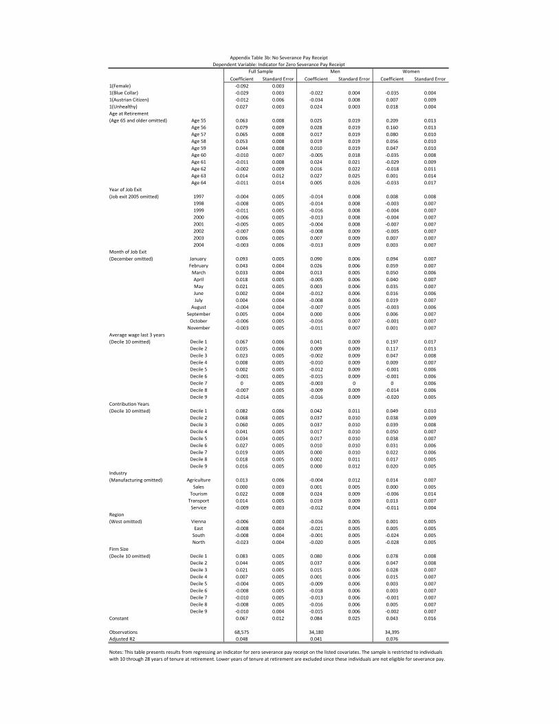
Notes: This table presents results from regressing an indicator for zero severance pay receipt on the listed covariates. The sample is restricted to individuals with 10 through 28 years of tenure at retirement. Lower years of tenure at retirement are excluded since these individuals are not eligible for severance pay.

Appendix Table 3b: No Severance Pay ReceiptDependent Variable: Indicator for Zero Severance Pay Receipt

Full Sample Men Women

10 Year Threshold 15 Year Threshold 20 Year Threshold 25 Year Threshold Weighted Average 10 Year Threshold 15 Year Threshold 20 Year Threshold 25 Year Threshold Weighted AverageExcess Mass

553.9370 543.4282 654.0662 399.7941 1149.0970 1488.9650 1305.9290 388.8052( 40.7909) ( 46.3852) ( 43.7540) ( 43.8715) ( 52.1589) ( 60.1331) ( 69.9948) ( 61.1119)

Fraction Constrained 0.7962 0.7277 0.6640 0.6299 0.6092 0.5771 0.5259 0.4279

( 0.0336) ( 0.0184) ( 0.0318) ( 0.0461) ( 0.0522) ( 0.0432) ( 0.0609) ( 0.1116)

Length of Delay 0.5176 0.4035 0.5222 0.4932 0.4582 0.5752 0.6603 0.4025

( 0.0550) ( 0.0432) ( 0.0593) ( 0.0980) ( 0.0500) ( 0.0573) ( 0.0904) ( 0.1264)

Point of Convergence 0.6667 1.4167 1.3333 1.1667 1.4167 1.4167 1.0833 1.0000

( 0.3756) ( 0.0956) ( 0.1582) ( 0.3998) ( 0.3376) ( 0.1746) ( 0.1486) ( 0.2579)

Elasticity, Lower Bound 0.0053 0.0023 0.0028 0.0022 0.0034 0.0060 0.0046 0.0044 0.0019 0.0048

( 0.0007) ( 0.0003) ( 0.0004) ( 0.0006) ( 0.0002) ( 0.0010) ( 0.0007) ( 0.0008) ( 0.0008) ( 0.0004)

Elasticity, Upper Bound 0.0081 0.0151 0.0108 0.0073 0.0107 0.0439 0.0194 0.0092 0.0066 0.0236

( 0.0010) ( 0.0021) ( 0.0020) ( 0.0016) ( 0.0008) ( 0.0219) ( 0.0040) ( 0.0021) ( 0.0028) ( 0.0072)

Tenure Weights3211 3072 2562 1530 4497 4631 3486 1226

Men WomenAppendix Table 4: Retirement Age Elasticities

Notes: Numbers in parentheses are bootstrapped standard errors based on 1000 replications. Tenure weights are used to compute the weighted average in the fifth column. The listed weights are the frequencies of retirement within one year following a tenure threshold; the weights are constructed by dividing the listed frequencies by the total of the frequencies.

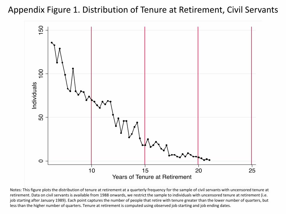
Appendix Figure 1. Distribution of Tenure at Retirement, Civil Servants

Notes: This figure plots the distribution of tenure at retirement at a quarterly frequency for the sample of civil servants with uncensored tenure at retirement. Data on civil servants is available from 1988 onwards, we restrict the sample to individuals with uncensored tenure at retirement (i.e. job starting after January 1989). Each point captures the number of people that retire with tenure greater than the lower number of quarters, but less than the higher number of quarters. Tenure at retirement is computed using observed job starting and job ending dates.

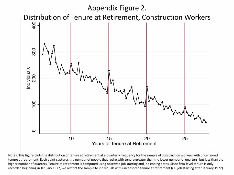
Notes: This figure plots the distribution of tenure at retirement at a quarterly frequency for the sample of construction workers with uncensored tenure at retirement. Each point captures the number of people that retire with tenure greater than the lower number of quarters, but less than the higher number of quarters. Tenure at retirement is computed using observed job starting and job ending dates. Since firm-level tenure is only recorded beginning in January 1972, we restrict the sample to individuals with uncensored tenure at retirement (i.e. job starting after January 1972).

Appendix Figure 2. Distribution of Tenure at Retirement, Construction Workers

Appendix Figure 3. Measurement Error in the Distribution of Tenure at Retirement

Notes: This figure plots the probability of having left over holiday days by tenure at retirement at a monthly frequency.

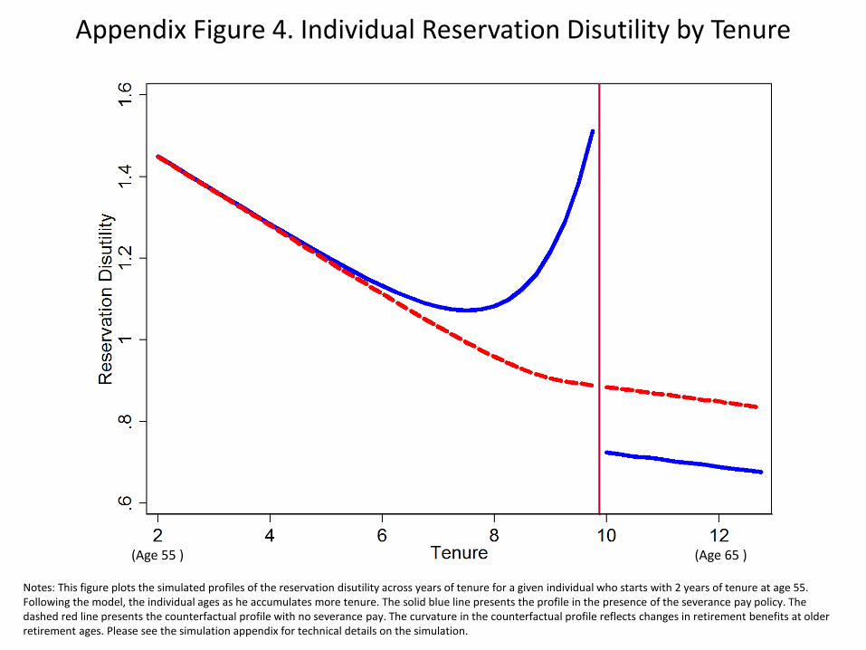
Notes: This figure plots the simulated profiles of the reservation disutility across years of tenure for a given individual who starts with 2 years of tenure at age 55. Following the model, the individual ages as he accumulates more tenure. The solid blue line presents the profile in the presence of the severance pay policy. The dashed red line presents the counterfactual profile with no severance pay. The curvature in the counterfactual profile reflects changes in retirement benefits at older retirement ages. Please see the simulation appendix for technical details on the simulation.

(Age 55 ) (Age 65 )

Appendix Figure 4. Individual Reservation Disutility by Tenure

Appendix Figure 5. Individual Retirement Hazard by Tenure

Notes: This figure plots the simulated profile of the retirement hazard rate (i.e. the probability of retirement conditional on remaining in the labor market) across years of tenure for a given individual who starts with 2 years of tenure at age 55. Following the model, the individual ages as he accumulates more tenure. The solid blue line presents the profile in the presence of the severance pay policy. The dashed red line presents the counterfactual profile with no severance pay. The curvature in the counterfactual profile reflects changes in retirement benefits at older retirement ages. Please see the simulation appendix for technical details on the simulation.

(Age 55 ) (Age 65 )

Appendix Figure 6. Average Retirement Hazard by Tenure

Notes: This figure plots the average simulated retirement hazard rate, conditional on remaining in the labor market, by tenure. The average retirement hazard rate at each level of tenure is computed by the following steps. First, retirement outcomes are computed for each simulated individual. Second, at each observed retirement, the reservation disutility and corresponding hazard rate are computed. Third, at each level of tenure at retirement, the average retirement hazard rate is computed by averaging over individuals retiring at different ages. The solid blue line and triangle present the hazard rates in the presence of the severance pay policy. The dashed red line and circle present the counterfactual hazard rates with no severance pay. Please see the simulation appendix for technical details on the simulation.

Appendix Figure 7. Simulated Distribution of Tenure at Retirement

Notes: This figure plots the simulated distribution of tenure at retirement based on simulated retirement outcomes for 10,000 simulated individuals. The solid blue line presents the distribution in the presence of the severance pay policy. The dashed red line presents the counterfactual distribution with no severance pay. Please see the simulation appendix for technical details on the simulation.

n pn p∆ ∆

⇒ =

Labor Supply

$

RL

Individual indifferent between retiring with sev. pay and R* and without sevpay at RL < R*

s

Individual strictly better off with sev. pay, no change in labor supply

dR* = R* - R

Appendix Figure 8. Optimal Retirement Choices with Severance Pay Notch

R*

Labor Supply

Indi

vidu

als

Appendix Figure 9a. Bunching Patterns, No Constraints

RL R*

Labor Supply

Indi

vidu

als

RL

Appendix Figure 9b. Bunching Patterns, Constant Fraction Constrained

R*

Labor Supply

Indi

vidu

als

RL R*

Appendix Figure 9c. Bunching Patterns, Heterogeneous Adjustment Costs