14. the multiple-equation gmm -...
TRANSCRIPT
14. The Multiple-Equation GMM
Hayashi p. 258-295
Advanced Econometrics I, Autumn 2010,Multiple-Equation GMM 1
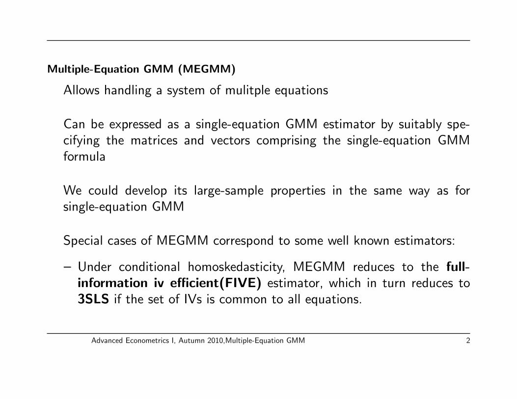
Multiple-Equation GMM (MEGMM)
Allows handling a system of mulitple equations
Can be expressed as a single-equation GMM estimator by suitably spe-cifying the matrices and vectors comprising the single-equation GMMformula
We could develop its large-sample properties in the same way as forsingle-equation GMM
Special cases of MEGMM correspond to some well known estimators:
– Under conditional homoskedasticity, MEGMM reduces to the full-information iv efficient(FIVE) estimator, which in turn reduces to3SLS if the set of IVs is common to all equations.
Advanced Econometrics I, Autumn 2010,Multiple-Equation GMM 2

Multiple-Equation GMM (cont’d)
– If we assume all the regressors are predetermined, 3SLS reduces toseemingly unrelated regressions (SUR), which in turn reduces tomultivariate regression when all the equations have the same regressors.
– The multiple-equation system can be written as an equation systemwith its coefficients constrained to be the same across equations. TheGMM estimator for this system is a special case of single-equationGMM.
– The GMM estimator with all the regressors predetermined and errorsconditionally homoskedastic is the random-effects(RE) estimator
– Thus, SUR and RE are equivalent estimators
Advanced Econometrics I, Autumn 2010,Multiple-Equation GMM 3

The Multiple-Equation Model (cont’d)
Assumption 4.1 (Linearity): There are M linear equations
yim = z′imδm + εim (m = 1, 2, ...,M ; i = 1, 2, ..., n)
where:n = sample size,
zim = Lm-dimensional vector of regressors,
δm = the conformable coefficient vector, and
εim = an unobservable error term in the m-th equation.
Oryim = z
′im
(1×Lm)
δm(Lm×1)
+ εim (m = 1, 2, ...,M ; i = 1, 2, ..., n)
Note: (i) No a priori assumption about cross equation error correlation, (ii)No cross equation parameter restriction
Advanced Econometrics I, Autumn 2010,Multiple-Equation GMM 4
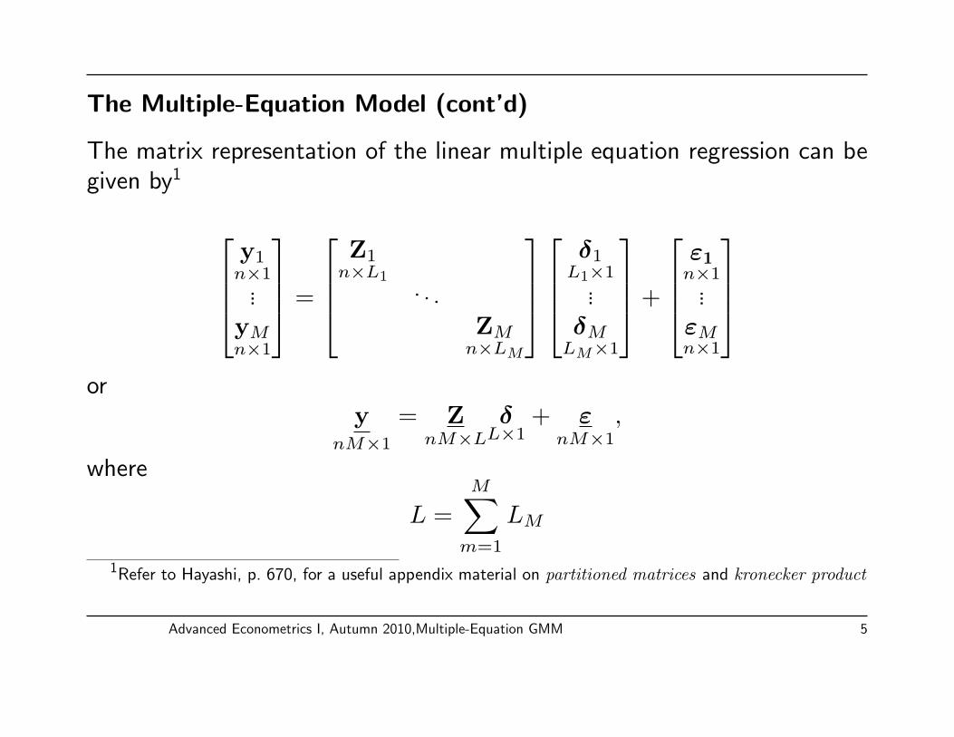
The Multiple-Equation Model (cont’d)
The matrix representation of the linear multiple equation regression can begiven by1
y1n×1
...yMn×1
=
Z1
n×L1. . .
ZMn×LM
δ1
L1×1...δM
LM×1
+
ε1n×1
...εMn×1
or
ynM×1
= ZnM×L
δL×1
+ εnM×1
,
where
L =
M∑m=1
LM
1Refer to Hayashi, p. 670, for a useful appendix material on partitioned matrices and kronecker product
Advanced Econometrics I, Autumn 2010,Multiple-Equation GMM 5
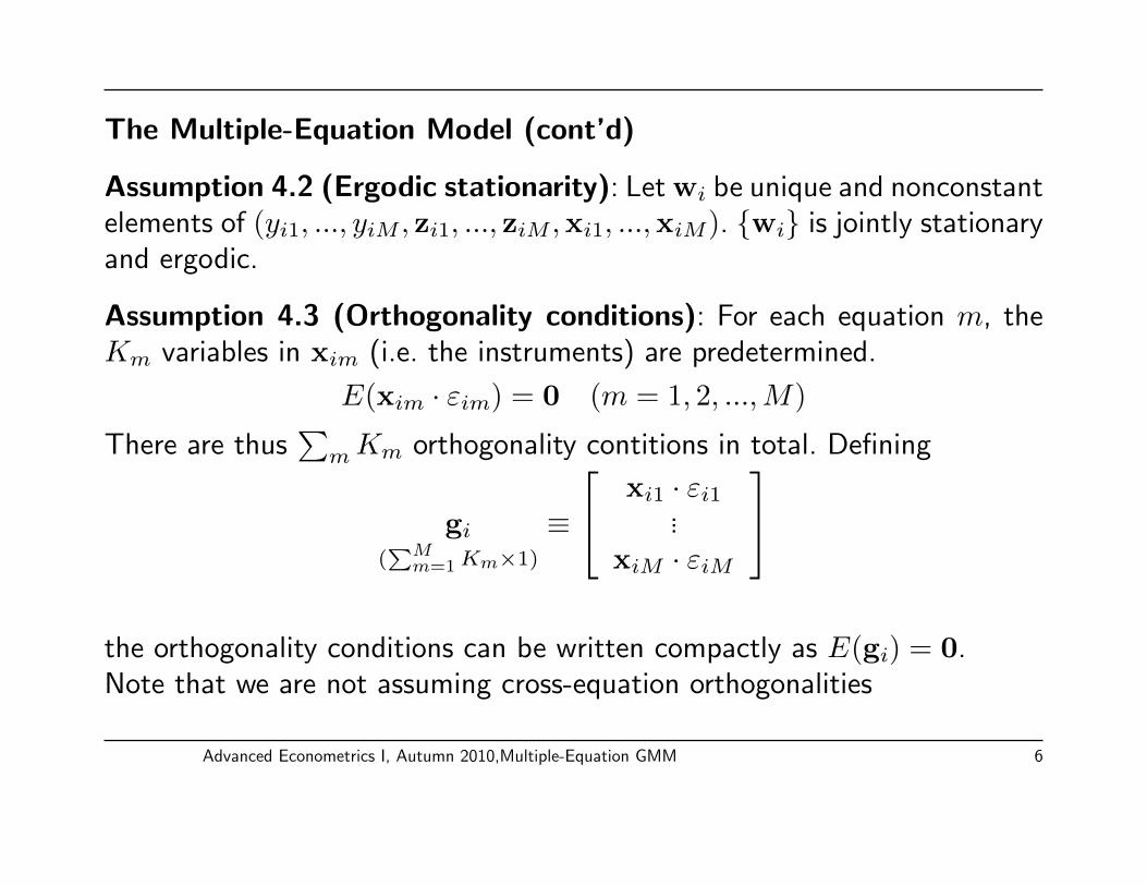
The Multiple-Equation Model (cont’d)
Assumption 4.2 (Ergodic stationarity): Let wi be unique and nonconstantelements of (yi1, ..., yiM , zi1, ..., ziM ,xi1, ...,xiM). {wi} is jointly stationaryand ergodic.
Assumption 4.3 (Orthogonality conditions): For each equation m, theKm variables in xim (i.e. the instruments) are predetermined.
E(xim · εim) = 0 (m = 1, 2, ...,M)
There are thus∑
mKm orthogonality contitions in total. Defining
gi
(∑M
m=1 Km×1)≡
xi1 · εi1...
xiM · εiM
the orthogonality conditions can be written compactly as E(gi) = 0.Note that we are not assuming cross-equation orthogonalities
Advanced Econometrics I, Autumn 2010,Multiple-Equation GMM 6

GMM Moment Conditions and Model identification
Given the orthogonality condition, identification could be established inmuch the same way as in the single-equation GMM case
g(wi; δ) ≡
xi1 · (yi1 − z′i1δ1)
...
xiM · (yiM − z′iMδM)
,
The orthogonality condition can be written as E[g(wi; δ)] = 0. Thecoefficient vector is identified if δ = δ is the only solution to the system ofequations
E[g(wi; δ)] = 0
Advanced Econometrics I, Autumn 2010,Multiple-Equation GMM 7

GMM Moment Conditions and Model identification (cont’d)
The expanded orthogonality conditions can be given as follows
E[g(wi; δ)] ≡
E[xi1 · (yi1 − z′i1δ1)]
...
E[xiM · (yiM − z′iM δM)]
=
E(xi1 · yi1)...
E(xiM · yiM)
− E(xi1z
′i1)δ1
...
E(xiMz′iM)δM
=
E(xi1 · yi1)...
E(xiM · yiM)
−E(xi1z
′i1) . . . 0
... . . . ...
0 . . . E(xiMz′iM)
δ1...δM
≡ σxy
(k×1)− Σxz
(K×L)δ
(L×1)
Advanced Econometrics I, Autumn 2010,Multiple-Equation GMM 8
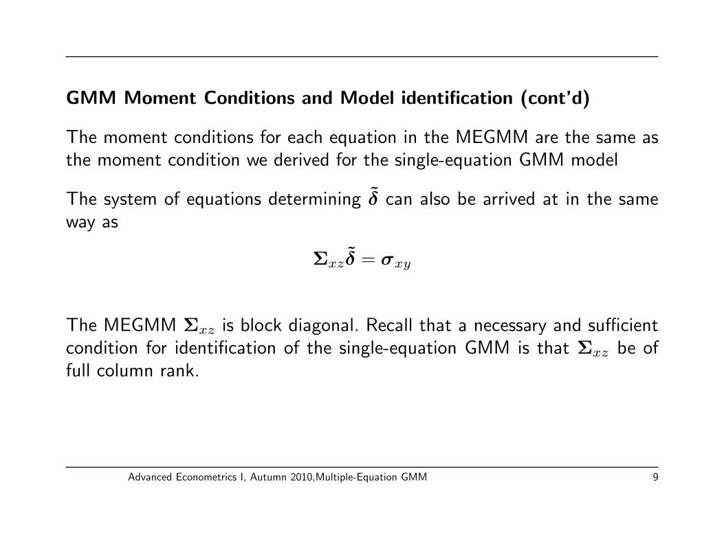
GMM Moment Conditions and Model identification (cont’d)
The moment conditions for each equation in the MEGMM are the same asthe moment condition we derived for the single-equation GMM model
The system of equations determining δ can also be arrived at in the sameway as
Σxzδ = σxy
The MEGMM Σxz is block diagonal. Recall that a necessary and sufficientcondition for identification of the single-equation GMM is that Σxz be offull column rank.
Advanced Econometrics I, Autumn 2010,Multiple-Equation GMM 9

GMM Moment Conditions and Model identification (cont’d)
If Km = Lm for m = 1, . . . ,M , then δ is exactly identified and δ1...δM
=
Σ−1x1z1σx1y1...
Σ−1xMzMσxMyM
If Km > Lm for some m, then solving
E[gi(δ)] = σxy(k×1)
− Σxz(K×L)
δ(L×1)
= 0
requires the rank condition
Assumption 4.4 (rank condition for identification): For each m(=
1, 2, . . . ,M), E(ximz′im)(Km × Lm) is of full column rank.
Advanced Econometrics I, Autumn 2010,Multiple-Equation GMM 10

GMM Moment Conditions and Model identification (cont’d)
That is, all coefficient vectors (δ1, . . . , δM) can be uniquely determined iffeach coefficient vector δM is uniquely determined.
This is the case if the orthogonality assumption holds for each equation.
Assumption 4.5 (gi is a martingale difference sequence with finitesecond moments):{gi} is a joint martingale difference sequence. E(gig
′i)
is nonsingular.
Note, as is also the case for ergodic stationarity, that this assumption isstronger than requiring the same for each equation.
We use S for Avar(g), the asymptotic variance of (g) (i.e. the variance ofthe limiting distribution of
√ng)
Advanced Econometrics I, Autumn 2010,Multiple-Equation GMM 11
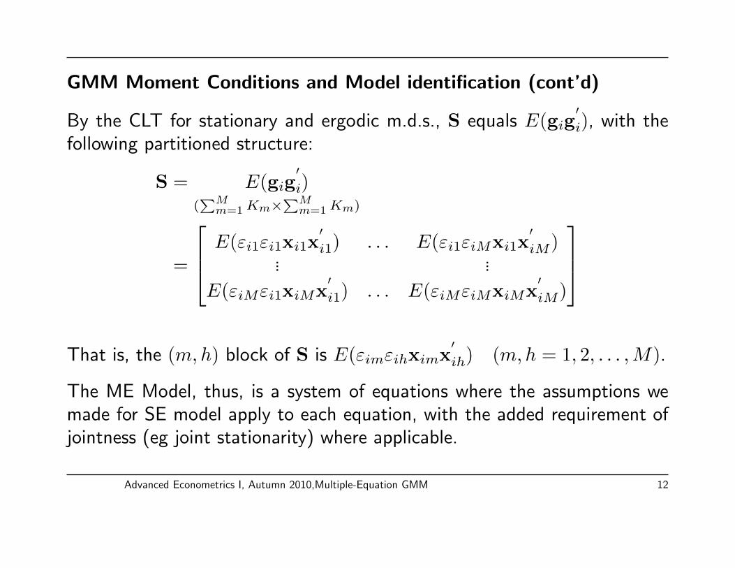
GMM Moment Conditions and Model identification (cont’d)
By the CLT for stationary and ergodic m.d.s., S equals E(gig′i), with the
following partitioned structure:
S = E(gig′i)
(∑M
m=1 Km×∑M
m=1 Km)
=
E(εi1εi1xi1x′i1) . . . E(εi1εiMxi1x
′iM)
... ...
E(εiMεi1xiMx′i1) . . . E(εiMεiMxiMx
′iM)
That is, the (m,h) block of S is E(εimεihximx
′ih) (m,h = 1, 2, . . . ,M).
The ME Model, thus, is a system of equations where the assumptions wemade for SE model apply to each equation, with the added requirement ofjointness (eg joint stationarity) where applicable.
Advanced Econometrics I, Autumn 2010,Multiple-Equation GMM 12

MEGMM Sample Moment
As in the SEGMM case, let δ be a hypothetical value of the true parametervector δ and define gn(δ) to be its sample analogue, which is given by:
gn(δ)(∑M
m=1 Km×1)=
1n
∑ni=1 xi1 · (yi1 − z
′i1δ1)
...1n
∑ni=1 xiM · (yiM − z
′iM δM)
=
1n
∑ni=1 xi1 · yi1
...1n
∑ni=1 xiM · yiM
− 1
n
∑ni=1 xi1z
′i1δ1
...1n
∑ni=1 xiMz
′iM δM
=
1n
∑ni=1 xi1 · yi1
...1n
∑ni=1 xiM · yiM
−1
n
∑ni=1 xi1z
′i1
. . .1n
∑ni=1 xiMz
′iM
δ1...δM
Advanced Econometrics I, Autumn 2010,Multiple-Equation GMM 13

MEGMM Sample Moment (cont’d)
Thus,
gn(δ)(∑M
m=1 Km×1)≡ sxy − Sxzδ,
where
sxy ≡
1n
∑ni=1 xi1 · yi1
...1n
∑ni=1 xiM · yiM
,Sxz ≡
[1n
∑ni=1 xi1z
′i1
. . . 1n
∑ni=1 xiMz
′iM
]
Orgn(δ)
(∑M
m=1 Km×1)= sxy
(K×1)− Sxz
(K×L)
δL×1)
Advanced Econometrics I, Autumn 2010,Multiple-Equation GMM 14

MEGMM,identification
If Km = Lm for m = 1, . . . ,M then X′mZm is a square matrix and so
δm = S−1xmzmSxmym, m = 1, . . . ,M
Therefore,δ = (δ1, . . . , δM)
′
SolvesSxy
(K×1)− Sxz
(K×L)
δ(L×1)
= 0
If each equation is identified and Km > Lm for some m, then it is notpossible to find some δ that solves the moment conditions.
Advanced Econometrics I, Autumn 2010,Multiple-Equation GMM 15

MEGMM,identification (cont’d)For the overidentified model, let W be a K×K positive definite symmetricmatrix given by
W =
W11 W12 . . . W1M
W′12 W22 . . . W2M
... ... . . . ...
W′1M W
′2M . . . WMM
Such that W→
pW. The GMM estimator then solves
δ(W) = argminδ
J(δ,W) = ngn(δ)′Wgn(δ)
= argminδ
n(sxy − Sxzδ
)′W(sxy − Sxzδ
)Advanced Econometrics I, Autumn 2010,Multiple-Equation GMM 16

MEGMM,identification (cont’d)
Straightforward but tedious algebra should give
δ(W) =(S′xzWSxz
)−1S′xzWsxy =
S′x1z1
W11Sx1z1 S′x1z1
W12Sx2z2 . . . S′x1z1
W1MSxMzM
S′x2z2
W′12Sx1z1 S
′x2z2
W21Sx2z2 . . . S′x2z2
W2MSxMzM... ... . . . ...
S′xMzM
W′1MSx1z1 S
′xMzM
W′2MSx2z2 . . . S
′xMzM
WMMSxMzM
−1
×
S′x1z1
∑Mm=1 W1msxmym
S′x2z2
∑Mm=1 W2msxmym
...
S′xMzM
∑Mm=1 WMmsxmym
Advanced Econometrics I, Autumn 2010,Multiple-Equation GMM 17

Multiple-Equation GMM Defined
The definition of the MEGMM estimator is the same as in the SEGMM,provided that the weighting matrix W is now
∑mKm ×
∑mKm.
Multiple-equation GMM estimator: δ(W) = (S′xzWSxz)
−1S′xzWsxy,
Its sampluing error: δ(W)− δ = (S′xzWSxz)
−1S′xzWg.
Features specific to the MEGMM are:
(i) sxy is a stacked vector,
(ii) Sxz is a block diagonal matrix,
(iii) accordingly, the size of the weighting matrix is∑
mKm×∑
mKm,
(iv) g, the sample mean of gi, is stacked vector, given by
Advanced Econometrics I, Autumn 2010,Multiple-Equation GMM 18

Multiple-Equation GMM Defined (cont’d)
g ≡ 1
n
n∑i=1
gi =
1n
∑ni=1 xi1 · εi1
...1n
∑ni=1 xiM · εiM
= gn(δ)
given these features, the MEGMM estimator
δ(W) = (S′xzWSxz)
−1S′xzWsxy
can be written out in full.
Required: the Wmh(Km ×Kh) has to be the (m,h) block of W(m,h =1, 2, . . . ,M)
[See Hayashi (2000), p. 267]
Advanced Econometrics I, Autumn 2010,Multiple-Equation GMM 19

MEGMM Asymptotics
The mechanics of asymptotics for multiple-equation GMM is similar to thatfor single-equation GMM so long as:
(i) δ,Σxz,S,gi, sxy, and Sxz are as defined for the multiple-equationGMM, and
(ii) the multiple-equaion GMM assumptions are used.
δ in the case of multiple equations is a stacked vector of parameterscomposed of coefficients from different equation.
We could conduct hypothesis testing involving cross-equation restrictions.
Advanced Econometrics I, Autumn 2010,Multiple-Equation GMM 20
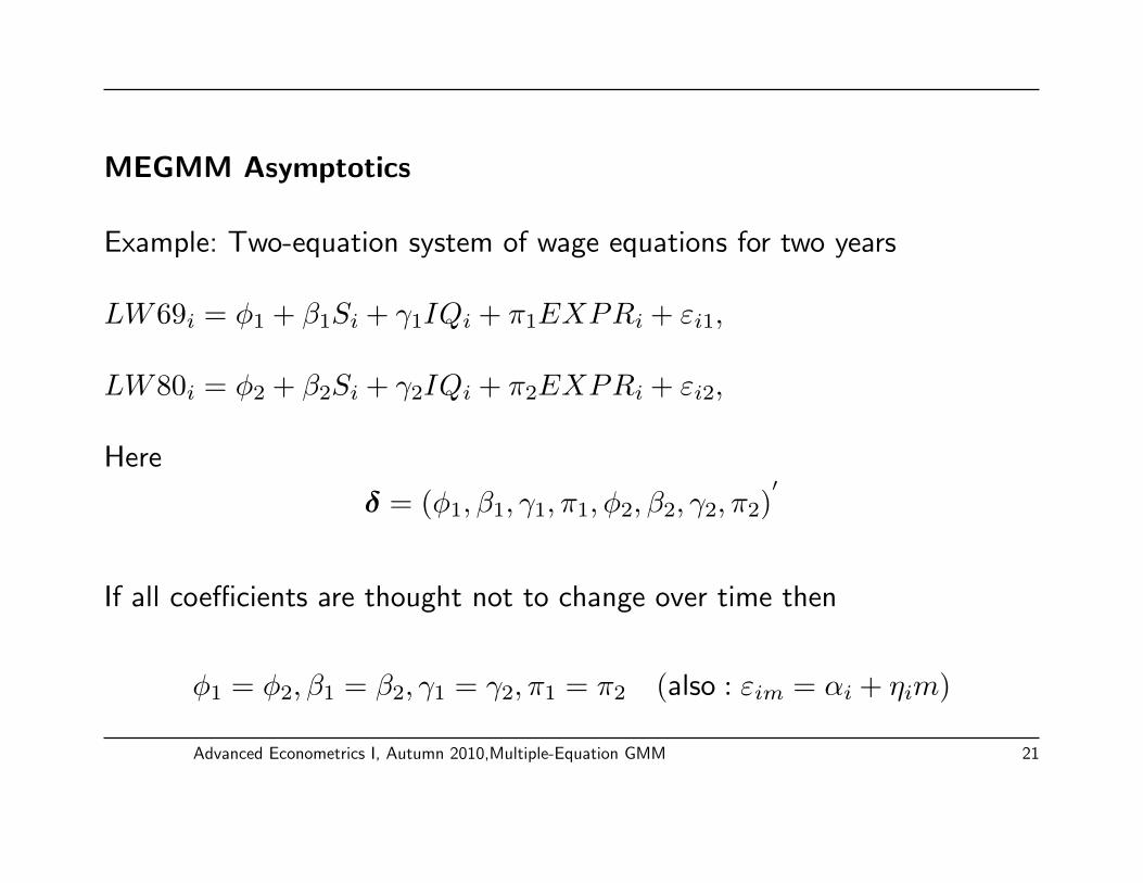
MEGMM Asymptotics
Example: Two-equation system of wage equations for two years
LW69i = φ1 + β1Si + γ1IQi + π1EXPRi + εi1,
LW80i = φ2 + β2Si + γ2IQi + π2EXPRi + εi2,
Here
δ = (φ1, β1, γ1, π1, φ2, β2, γ2, π2)′
If all coefficients are thought not to change over time then
φ1 = φ2, β1 = β2, γ1 = γ2, π1 = π2 (also : εim = αi + ηim)
Advanced Econometrics I, Autumn 2010,Multiple-Equation GMM 21

We could test this as:
H0 : φ1 = φ2, β1 = β2, γ1 = γ2, and, π1 = π2
The Hypothesis can be written as Rδ = r, where.
R =
1 0 0 0 −1 0 0 00 1 0 0 0 −1 0 00 0 1 0 0 0 −1 00 0 0 1 0 0 0 −1
, r =
0000
.
Advanced Econometrics I, Autumn 2010,Multiple-Equation GMM 22

MEGMM Asymptotics
(Test of overidentifying restriction) The number of orthogonality conditionsis K =
∑mKm and the number of coefficients is L =
∑mLm. The degrees
of freedom for the J statistic is thus K − L =∑
mKm −∑
mLm.
Proposition 4.1 (consistent estimation of contemporaneous errorcross-equation moments): Let δm be a consistent estimator of δm, and
let εim ≡ yim − z′imδm be the implied residual for m = 1, 2, . . . ,M . Under
Assumptions 4.1 and 4.2, plus the assumption that E(zimz′ih) exists and is
finite for all m,h(= 1, 2, . . . ,M),
σmh →pσmh,
whereσmh ≡
1
n
n∑i=1
εimε′ih and σmh ≡ E(εimεih)
Provided that E(εimεih) exists and is finite.
Advanced Econometrics I, Autumn 2010,Multiple-Equation GMM 23
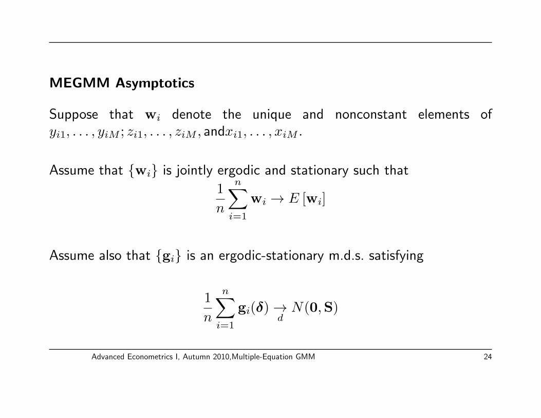
MEGMM Asymptotics
Suppose that wi denote the unique and nonconstant elements ofyi1, . . . , yiM ; zi1, . . . , ziM , andxi1, . . . , xiM .
Assume that {wi} is jointly ergodic and stationary such that
1
n
n∑i=1
wi → E [wi]
Assume also that {gi} is an ergodic-stationary m.d.s. satisfying
1
n
n∑i=1
gi(δ)→dN(0,S)
Advanced Econometrics I, Autumn 2010,Multiple-Equation GMM 24

where, as before
S = E[gi(δ)gi(δ′)]
=
E[xi1x
′i1ε
2i1] E[xi1x
′i2εi1εi2] . . . E[xi1x
′iMεi1εiM ]
E[xi2x′i1εi2εi1] E[xi2x
′i2ε
2i2] . . . E[xi2x
′iMεi2εiM ]
... ... . . . ...
E[xiMx′i1εiMεi1] E[xiMx
′i2εiMεi2] . . . E[xiMx
′iMε
2iM ]
Assumption 4.6(finite fourth moments): E[(ximk · · · zihj)2] exists andis finite for all k(= 1, 2, . . . ,Km), j(= 1, 2, . . . , Lh),m, h(= 1, 2, . . . ,M),where ximk is the k-th element of xim and zihj is the j-th element of zih.
Advanced Econometrics I, Autumn 2010,Multiple-Equation GMM 25

MEGMM Asymptotics
Estimation of S: the multiple-equation version formula for consistentlyestimating S is given by
S =
S11 S12 . . . S1M
S′12 S22 . . . S2M... ... . . . ...
S′1M S
′2M . . . SMM
where
Smh =1
n
n∑i=1
ximx′ihεimεih
Proposition 4.2 (consistent estimation of S, the asymptotic varianceof g): Let εm be a consistent estimator of εm, and let εim ≡ yim − z
′imδm
be the implied residual for m = 1, 2, . . . ,M .
Advanced Econometrics I, Autumn 2010,Multiple-Equation GMM 26

MEGMM Asymptotics
Under Assumptions 4.1, 4.2, and 4.6, S is consistent for S.
Potential initial consistent estimators of δ:
1. δ(IK) = (δ1(IK1)′, . . . , δM(IKM
)′)′
2. Single equation efficient GMM estimators:
δm(S−1mm), m = 1, . . . ,M
Advanced Econometrics I, Autumn 2010,Multiple-Equation GMM 27

MEGMM Asymptotics
Since S is consistent for S, the MEGMM estimator that uses S−1 asthe weighting matrix, δ(S−1), is an efficient MEGMM estimator withminimum asymptotic variance.
Thus,
Avar(δ(S−1)) = (Σ′xzS−1Σxz),
Avar(δ(S−1)) = (S′xzS−1Sxz)
−1.
Advanced Econometrics I, Autumn 2010,Multiple-Equation GMM 28

Single- vs. Multiple-Equation GMM
Single-equation GMM is a special case of multiple-equation GMM
In SEGMM, apply GMM on each equation separately with equationspecific weight matrix Wmm; so that
δm(Wmm) = (S′xmzmWmmSxmzm)
−1S′xmzmWmmSxmym
m = 1, . . . ,M
This is MEGMM with a block diagonal weight matrix
W = diag(W11, . . . ,WMM)
Question: When is multiple-equation efficient GMM equivalent to singleequation efficient GMM?
Advanced Econometrics I, Autumn 2010,Multiple-Equation GMM 29

Single- vs. Multiple-Equation GMM
Two cases:
1. Each equation is just identified ⇒ the weight matrix does not matter(obvious case)
2. At least one equation is overidentified but S = E[gi(δ)gi(δ)′] is block
diagonal (not so obvious case)
S = diag(S11, . . . ,SMM)
= diag(E[xi1x′i1ε
2i1], . . . , E[xiMx
′iMε
2iM ])
That is, if the equations are unrelated as in
E[ximx′ihεimεih] = 0 for all m 6= h
Advanced Econometrics I, Autumn 2010,Multiple-Equation GMM 30
15. Special Cases of MEGMM: FIVE, 3SLSand SUR
Hayashi, pp. 274-294
Advanced Econometrics I, Autumn 2010,Multiple-Equation GMM 31
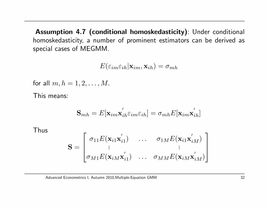
Assumption 4.7 (conditional homoskedasticity): Under conditionalhomoskedasticity, a number of prominent estimators can be derived asspecial cases of MEGMM.
E(εimεih|xim,xih) = σmh
for all m,h = 1, 2, . . . ,M.
This means:
Smh = E[ximx′ihεimεih] = σmhE[ximx
′ih]
Thus
S =
σ11E(xi1x′i1) . . . σ1ME(xi1x
′iM)
... ...
σM1E(xiMx′i1) . . . σMME(xiMx
′iM)
Advanced Econometrics I, Autumn 2010,Multiple-Equation GMM 32

Full-Information Instrumental Variables Efficient (FIVE)
An estimator of S in this case is
S =
σ11 · (1n∑n
i=1 xi1x′i1) . . . σ1M · (1n
∑ni=1 xi1x
′iM)
... ...
σM1 · (1n∑n
i=1 xiMx′i1) . . . σMM · (1n
∑ni=1 xiMx
′iM)
,where, for some consistent estimator δm of δ,
σmh ≡1
n
n∑i=1
εimεih; εim ≡ yim − z′imδm (m,h = 1, ,M)
Advanced Econometrics I, Autumn 2010,Multiple-Equation GMM 33

FIVE
- σmh →p σmh provided that E(zimz′ih) (and assumptions 4.1 and 4.2)
- 1n
∑i ximx
′ih →p E(ximx
′ih), which exists and is finite (by ergodic
stationarity)
Therefore, S is consistent for S.
The FIVE estimator of δ, denoted δFIV E, is thus
δFIV E ≡ δ(S−1)
Advanced Econometrics I, Autumn 2010,Multiple-Equation GMM 34

FIVE
Large-sample properties of FIVE:
Under the conditions of
a. Assumptions 4.1-4.5 and 4.7,b. E(zimz
′ih) exists and finite for all m,h(= 1, 2, . . . ,M), and
c. S and S given above:
We have large-sample properties of FIVE in that
i. S→p S;
ii. δFIV E ≡ δ(S−1) is consistent, asymptotically normal, and efficient with
Avar(δ(S−1)) = (Σ′xzS−1Σxz)
−1;
iii.
Avar(δ(S−1)) = (S′xz
ˆS−1Sxz)−1 is consistent for Avar(δFIVE)
Advanced Econometrics I, Autumn 2010,Multiple-Equation GMM 35

FIVE
iv. Sargan’s Statistic:
J(δFIVE, S−1) ≡ n · gn(δFIVE)
′S−1gn(δFIVE)→
dχ2
(∑m
(Km − Lm)
),
wheregn(·) = gn(δ)
(∑M
m=1 Km×1)≡ sxy − Sxzδ
The initial estimator δm needed to calculate S is usually the 2SLSestimator.
Advanced Econometrics I, Autumn 2010,Multiple-Equation GMM 36

Three-Stage Least Squares (3SLS)
Assumptions:
(a) Conditional homoskedasticity
E[εimεih|xim,xih] = σmh
for all m,h = 1, 2, . . . ,M.
⇒ Smh = E[ximx′ihεimεih] = σmhE[ximx
′ih]
(b) Common set of instruments across all equations
xi1 = xi2 = . . . = xim = xik×1
Advanced Econometrics I, Autumn 2010,Multiple-Equation GMM 37

3SLS
The 3SLS moment conditions can be given by
gi(Mk×1)
=
xiεi1...
xiεiM
= εi ⊗ xi, with εi(M×1)
≡
εi1...εiM
The 3SLS Efficient Weight matrix is
S3SLS(Mk×Mk)
=
σ11E[xix
′i] σ12E[xix
′i] . . . σ1ME[xix
′i]
σ12E[xix′i] σ22E[xix
′i] . . . σ2ME[xix
′i]
... ... . . . ...
σ1ME[xix′i] σ2ME[xix
′i] . . . σMME[xix
′i]
Advanced Econometrics I, Autumn 2010,Multiple-Equation GMM 38

3SLS
Or compactly as
S3SLS(Mk×Mk)
= Σ(M×M)
⊗ E[xix′i]
(k×k),
where
Σ(M×M)
= E[εiε′i] =
σ11 σ12 . . . σ1M
σ12 σ22 . . . σ2M... ... . . . ...
σ1M σ2M . . . σMM
Then
S−13SLS = Σ−1(M×M)
⊗ E[xix′i]−1
(k×k)
Advanced Econometrics I, Autumn 2010,Multiple-Equation GMM 39
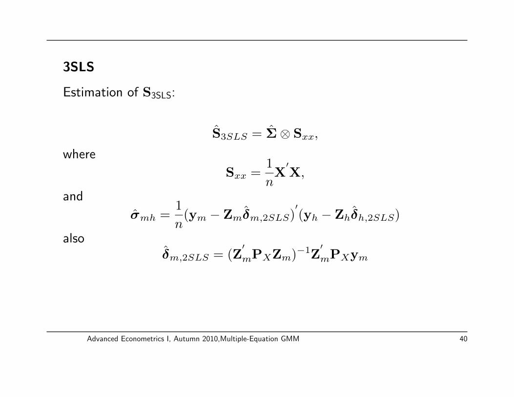
3SLS
Estimation of S3SLS:
S3SLS = Σ⊗ Sxx,
where
Sxx =1
nX′X,
and
σmh =1
n(ym − Zmδm,2SLS)
′(yh − Zhδh,2SLS)
alsoδm,2SLS = (Z
′mPXZm)−1Z
′mPXym
Advanced Econometrics I, Autumn 2010,Multiple-Equation GMM 40
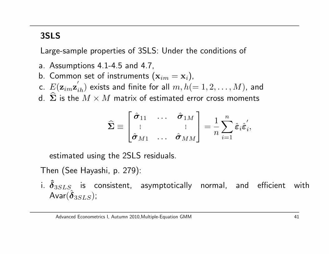
3SLS
Large-sample properties of 3SLS: Under the conditions of
a. Assumptions 4.1-4.5 and 4.7,b. Common set of instruments (xim = xi),
c. E(zimz′ih) exists and finite for all m,h(= 1, 2, . . . ,M), and
d. Σ is the M ×M matrix of estimated error cross moments
Σ ≡
σ11 . . . σ1M... ...
σM1 . . . σMM
=1
n
n∑i=1
εiε′
i,
estimated using the 2SLS residuals.
Then (See Hayashi, p. 279):
i. δ3SLS is consistent, asymptotically normal, and efficient withAvar(δ3SLS);
Advanced Econometrics I, Autumn 2010,Multiple-Equation GMM 41

Large-Sample properties of 3SLS
ii. The estimated asymptotic variance Avar(δ3SLS) is consistent forAvar(δ3SLS);
iii. Sargan’s statistic
J(δ3SLS, S−1) ≡ n · gn(δ3SLS)
′S−1gn(δ3SLS)→
dχ2
(MK −
∑m
Lm)
),
where
S = Σ⊗ (1
n
∑i
xix′i),Kis the number of common instruments, and
gn(·) = gn(δ)(∑M
m=1 Km×1)≡ sxy − Sxzδ
Advanced Econometrics I, Autumn 2010,Multiple-Equation GMM 42
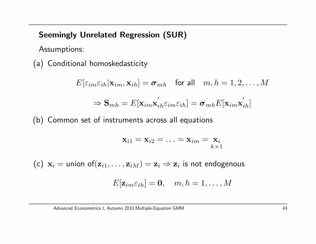
Seemingly Unrelated Regression (SUR)
Assumptions:
(a) Conditional homoskedasticity
E[εimεih|xim,xih] = σmh for all m,h = 1, 2, . . . ,M
⇒ Smh = E[ximx′ihεimεih] = σmhE[ximx
′ih]
(b) Common set of instruments across all equations
xi1 = xi2 = . . . = xim = xik×1
(c) xi = union of(zi1, . . . , ziM) = zi ⇒ zi is not endogenous
E[zimεih] = 0, m, h = 1, . . . ,M
Advanced Econometrics I, Autumn 2010,Multiple-Equation GMM 43
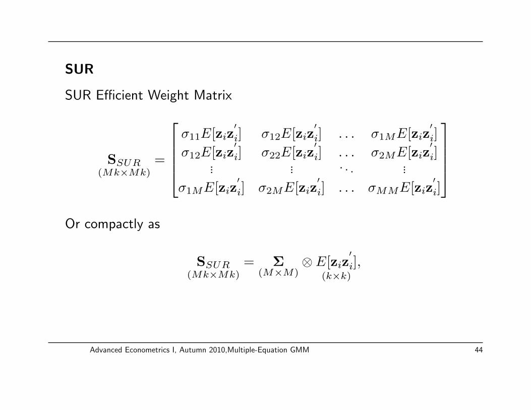
SUR
SUR Efficient Weight Matrix
SSUR(Mk×Mk)
=
σ11E[ziz
′i] σ12E[ziz
′i] . . . σ1ME[ziz
′i]
σ12E[ziz′i] σ22E[ziz
′i] . . . σ2ME[ziz
′i]
... ... . . . ...
σ1ME[ziz′i] σ2ME[ziz
′i] . . . σMME[ziz
′i]
Or compactly as
SSUR(Mk×Mk)
= Σ(M×M)
⊗ E[ziz′i]
(k×k),
Advanced Econometrics I, Autumn 2010,Multiple-Equation GMM 44

SUR
Estimating SSUR
SSUR = ΣSUR ⊗ Szz,
where
Szz =1
nZ′Z,
and
σmh =1
n(ym − Zmδm,OLS)
′(yh − Zhδh,OLS)
alsoδm,OLS = (Z
′mZm)−1Z
′mym
Advanced Econometrics I, Autumn 2010,Multiple-Equation GMM 45

Large-Sample properties of SUR
Under the conditions of
a. Assumptions 4.1-4.5 and 4.7,b. Common set of instruments (xim = xi),c. xi = union of(zi1, . . . , ziM)
d. Σ is the M ×M matrix of estimated error cross moments
Σ ≡
σ11 . . . σ1M... ...
σM1 . . . σMM
=1
n
n∑i=1
εiε′
i,
estimated using the OLS residuals.
Then (See Hayashi, p. 281):
i. δSUR is consistent, asymptotically normal, and efficient with Avar(δSUR);
Advanced Econometrics I, Autumn 2010,Multiple-Equation GMM 46
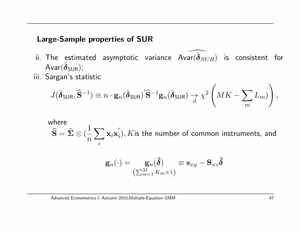
Large-Sample properties of SUR
ii. The estimated asymptotic variance Avar(δSUR) is consistent forAvar(δSUR);
iii. Sargan’s statistic
J(δSUR, S−1) ≡ n · gn(δSUR)
′S−1gn(δSUR)→
dχ2
(MK −
∑m
Lm)
),
where
S = Σ⊗ (1
n
∑i
xix′i),Kis the number of common instruments, and
gn(·) = gn(δ)(∑M
m=1 Km×1)≡ sxy − Sxzδ
Advanced Econometrics I, Autumn 2010,Multiple-Equation GMM 47