ancillary services shortage pricing - nyiso
TRANSCRIPT
Ancillary Services Shortage Pricing A Report by the New York Independent System Operator
December 2019
DRAFT PURPOSES ONLY Ancillary Services Shortage Pricing | 2
Table of Contents INTRODUCTION....................................................................................................................................................................................3
ANCILLARY SERVICES SHORTAGE PRICING .......................................................................................................................................4 Current Reserves Shortage Pricing in NYISO..................................................................................................................5
Trade-Offs ............................................................................................................................................................................8
Neighboring ISO/RTO Demand Curve Levels .................................................................................................................9
HISTORICAL SHORTAGE PRICING ANALYSIS .................................................................................................................................. 11 Frequency of NYCA 30-Minute Reserve Shortages .................................................................................................... 11
Persistent Reserve Shortage Analysis .......................................................................................................................... 12
ANALYSIS OF SEPTEMBER 3, 2018 .................................................................................................................................................. 13 Emergency Energy Purchases from Ontario ................................................................................................................ 13
September 3, 2018 Day Rerun Analysis...................................................................................................................... 14
UNDERSTANDING VALUE OF LOST LOAD....................................................................................................................................... 15 VOLL Background ............................................................................................................................................................ 15
VOLL Based Shortage Pricing Consideration............................................................................................................... 15
VOLL Estimation for New York ....................................................................................................................................... 16
Loss of Load Probability ................................................................................................................................................. 17
LOLP Estimation Methodologies ................................................................................................................................... 17
LOLP Estimation for New York ....................................................................................................................................... 18
CONCLUSION ..................................................................................................................................................................................... 20
APPENDIX A: SHORTAGE PRICING IN OTHER ISOS/RTOS ............................................................................................................. 21 APPENDIX B: HISTORICAL SHORTAGE PRICING ANALYSIS ........................................................................................................... 23
Frequency of Ancillary Services Shortages .................................................................................................................. 23
APPENDIX C: ANALYSIS OF SEPTEMBER 3, 2018 ........................................................................................................................... 25
APPENDIX D: VALUE OF LOST LOAD ............................................................................................................................................... 29 VOLL Background ............................................................................................................................................................ 29
VOLL Estimation for New York ....................................................................................................................................... 30
VOLL Approach for Reserve Shortage Pricing and its Adoption across Other ISOs/RTOs..................................... 31
LOLP Estimation for New York ....................................................................................................................................... 33
Calculation of ORDCs Using VOLL and LOLP Construct ............................................................................................. 37
DRAFT PURPOSES ONLY Ancillary Services Shortage Pricing | 3
Introduction Ancillary services support the transmission of energy from resources to loads, while maintaining
reliable operations. Effective pricing of these ancillary services are crucial to reflect system conditions and
operational needs.
Well-structured market designs with simultaneously co-optimized energy and ancillary services
including shortage pricing provide incentives to ensure needed resources remain available for providing
ancillary services and maintaining bulk power system reliability. The NYISO is examining its ancillary
services shortage pricing to ensure that New York’s wholesale markets continue to support the necessary
incentives for investment in, and maintenance of, resources that the bulk power system needs to maintain
reliability.
In a future with increased penetration of weather-dependent generation technologies, the grid will
need responsive and flexible resources to address expected and unexpected changes in net load. Shortage
pricing assists in providing incentives for resource flexibility and responsiveness. It provides a mechanism
for effectively valuing needed reliability services during times when supply is short by providing
market signals for resources to provide the products necessary for reliability. Shortage pricing for
reserves in the NYISO-administered markets is effectuated through the use of Operating Reserve Demand
Curves (ORDCs). Each ORDC represents the value of the reserve product over a range of reserve shortage
levels.
The Market Monitoring Unit (MMU) has recommended that NYISO assess modifications to the current
reserve shortage pricing values since the 2017 State of Market Report (SOM).1 Further expanding on this
recommendation in the 2018 SOM,2 the MMU noted that:
■ NYISO’s ORDCs are lower than the value of holding the reserves, based on the implied value of lost load; and
■ NYISO’s ORDC steps are low relative to neighboring markets in PJM and ISO-NE. Given the MMU’s recommendations and the importance of attributes such as resource flexibility and
responsiveness, the NYISO commenced an evaluation of its current shortage pricing structure.3
1 See Recommendation 2017-2 in the 2017 State of the Market Report, located at the following link: https://www.nyiso.com/documents/20142/2223763/2017-State-Of-The-Market-Report.pdf/cd4ee8a0-1989-dfa0-b53e-2d642c65e46d 2 See Recommendation 2017-2 in the 2018 State of the Market Report, located at the following link: https://www.nyiso.com/documents/20142/2223763/2018-State-of-the-Market-Report.pdf/b5bd2213-9fe2-b0e7-a422-
d4071b3d014b?t=1557344025932 3 The last comprehensive review of the NYISO’s shortage pricing values was completed 2015. This review resulted in the addition of the
Southeastern New York reserve region, an increase in the total reserve requirement statewide, and revised shortage pricing values. See Docket No. ER15-1061-000, New York Independent System Operator, Inc., Proposed Tariff Revisions to Ancillary Service Demand Curves and the Transmission Shortage Cost (February 18, 2015); and New York Independent System Operator, Inc., 151 FERC ¶ 61,057 (2015).
DRAFT PURPOSES ONLY Ancillary Services Shortage Pricing | 4
This report provides an overview of the assessment conducted by the NYISO to evaluate current
reserve shortage pricing values. The NYISO considered the effectiveness of the current shortage pricing
levels in supporting reliable operations by evaluating market prices and operator actions during shortage
and other adverse system operating conditions. The NYISO also considered potential approaches for
valuing reserves based on the value of lost load in its assessment of current reserve shortage pricing values.
Additionally, an overview of the importance of shortage pricing and its adoption in the NYISO, ISO-NE and
PJM markets is included in this report. The study concludes with key observations about the current
shortage pricing in the NYISO markets, and recommends further collaboration with stakeholders on this
topic.
Ancillary Services Shortage Pricing Ancillary services4 include: (a) Regulation Service, which is used to account for very short-term
deviations between supply and demand (6-seconds); (b) Spinning Reserves, which is capacity held in
reserve and synchronized to the grid and able to respond within 10-minutes; and, (c) 10-minute total
reserves, which includes Spinning Reserves and 10-minute Non-Synchronized Reserves. 10-minute Non-
Synchronized Reserves is capacity that is not synchronized to the grid, but can be started, synchronized,
and change output level (or reduce demand) within 10-minutes; and (d) 30-minute Reserves, which
include synchronized and non-synchronized capacity that is available to respond within 30-minutes.
Collectively, these and other ancillary services help maintain system frequency, maintain a close balance
between the supply and demand of electricity, and ensure continuous delivery of energy when unexpected
events arise that impact such service.
Shortage pricing is the method employed to efficiently price energy and ancillary services when market
conditions are tight. It is a mechanism employed by the NYISO that establishes a price when the system is
deficient (or short) of operating reserves or the cost of procuring reserves exceeds specified values.
Administrative shortage pricing helps to reflect the increasing value of flexible supply (or demand) as
available reserve capability is depleted.
The purpose of shortage pricing in the short-term is to incent availability and flexibility of existing
resources and support system reliability. In the longer-term, shortage pricing helps to inform efficient
resource investment decisions to build and maintain flexible resources.
4 Capitalized terms not otherwise defined herein shall have the meaning specified in the Market Administration and Control Area Services (Services
Tariff) and Open Access Transmission Tariff (OATT).
DRAFT PURPOSES ONLY Ancillary Services Shortage Pricing | 5
Current Reserves Shortage Pricing in NYISO
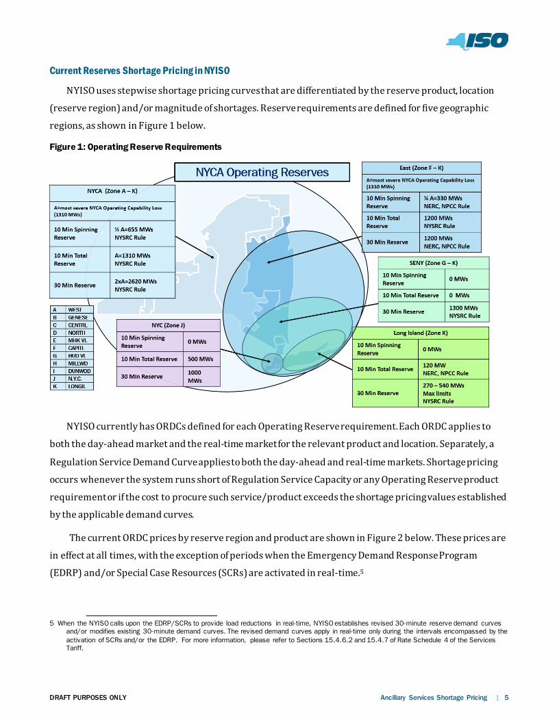
NYISO uses stepwise shortage pricing curves that are differentiated by the reserve product, location
(reserve region) and/or magnitude of shortages. Reserve requirements are defined for five geographic
regions, as shown in Figure 1 below.
Figure 1: Operating Reserve Requirements
NYISO currently has ORDCs defined for each Operating Reserve requirement. Each ORDC applies to
both the day-ahead market and the real-time market for the relevant product and location. Separately, a
Regulation Service Demand Curve applies to both the day-ahead and real-time markets. Shortage pricing
occurs whenever the system runs short of Regulation Service Capacity or any Operating Reserve product
requirement or if the cost to procure such service/product exceeds the shortage pricing values established
by the applicable demand curves.
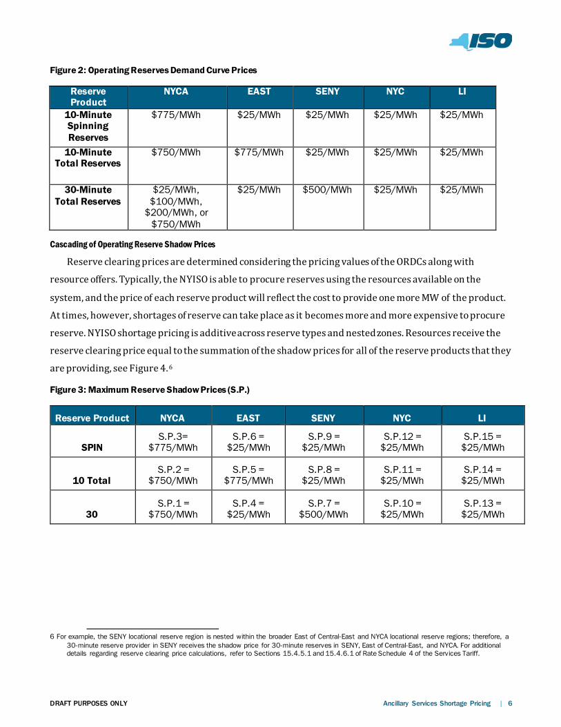
The current ORDC prices by reserve region and product are shown in Figure 2 below. These prices are
in effect at all times, with the exception of periods when the Emergency Demand Response Program
(EDRP) and/or Special Case Resources (SCRs) are activated in real-time.5
5 When the NYISO calls upon the EDRP/SCRs to provide load reductions in real-time, NYISO establishes revised 30-minute reserve demand curves
and/or modifies existing 30-minute demand curves. The revised demand curves apply in real-time only during the intervals encompassed by the activation of SCRs and/or the EDRP. For more information, please refer to Sections 15.4.6.2 and 15.4.7 of Rate Schedule 4 of the Services Tariff.
DRAFT PURPOSES ONLY Ancillary Services Shortage Pricing | 6
Figure 2: Operating Reserves Demand Curve Prices
Reserve Product
NYCA EAST SENY NYC LI
10-Minute Spinning Reserves
$775/MWh $25/MWh $25/MWh $25/MWh $25/MWh
10-Minute Total Reserves
$750/MWh $775/MWh $25/MWh $25/MWh $25/MWh
30-Minute Total Reserves
$25/MWh, $100/MWh,
$200/MWh, or $750/MWh
$25/MWh $500/MWh $25/MWh $25/MWh
Cascading of Operating Reserve Shadow Prices
Reserve clearing prices are determined considering the pricing values of the ORDCs along with
resource offers. Typically, the NYISO is able to procure reserves using the resources available on the
system, and the price of each reserve product will reflect the cost to provide one more MW of the product.
At times, however, shortages of reserve can take place as it becomes more and more expensive to procure
reserve. NYISO shortage pricing is additive across reserve types and nested zones. Resources receive the
reserve clearing price equal to the summation of the shadow prices for all of the reserve products that they
are providing, see Figure 4.6
Figure 3: Maximum Reserve Shadow Prices (S.P.)
Reserve Product NYCA EAST SENY NYC LI
SPIN S.P.3=
$775/MWh S.P.6 =
$25/MWh S.P.9 =
$25/MWh S.P.12 =
$25/MWh S.P.15 =
$25/MWh
10 Total S.P.2 =
$750/MWh S.P.5 =
$775/MWh S.P.8 =
$25/MWh S.P.11 =
$25/MWh S.P.14 =
$25/MWh
30 S.P.1 =
$750/MWh S.P.4 =
$25/MWh S.P.7 =
$500/MWh S.P.10 =
$25/MWh S.P.13 =
$25/MWh
6 For example, the SENY locational reserve region is nested within the broader East of Central-East and NYCA locational reserve regions; therefore, a
30-minute reserve provider in SENY receives the shadow price for 30-minute reserves in SENY, East of Central-East, and NYCA. For additional details regarding reserve clearing price calculations, refer to Sections 15.4.5.1 and 15.4.6.1 of Rate Schedule 4 of the Services Tariff.
DRAFT PURPOSES ONLY Ancillary Services Shortage Pricing | 7
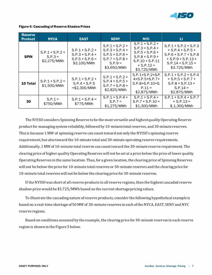
Figure 4: Cascading of Reserve Shadow Prices
Reserve Product NYCA EAST SENY NYC LI
SPIN S.P.1 + S.P.2 +
S.P.3 = $2,275/MWh
S.P.1 + S.P.2 + S.P.3 + S.P.4 + S.P.5 + S.P.6 = $3,100/MWh
S.P.1 + S.P.2 + S.P.3 + S.P.4 + S.P.5 + S.P.6 + S.P.7 + S.P.8 +
S.P.9 = $3,650/MWh
S.P.1 + S.P.2 + S.P.3 + S.P.4 + S.P.5 + S.P.6 + S.P.8 + S.P.9 + S.P.10 + S.P.11
+ S.P.12 = $3,725/MWh
S.P.1 + S.P.2 + S.P.3 + S.P.4 + S.P.5 +
S.P.6 + S.P.7 + S.P.8 + S.P.9 + S.P.13 + S.P.14 + S.P.15 =
$3.725/MWh
10 Total S.P.1 + S.P.2 = $1,500/MWh
S.P.1 + S.P.2 + S.P.4 + S.P.5
=$2,300/MWh
S.P.1 + S.P.2 + S.P.4 + S.P.5 + S.P.7 + S.P.8 = $2,825/MWh
S.P.1+S.P.2+S.P.4+S.P.5+S.P.7+S.P.8+S.P.10+S.
P.11 = $2,875/MWh
S.P.1 + S.P.2 + S.P.4 + S.P.5 + S.P.7 + S.P.8 + S.P.13 +
S.P.14 = $2,875/MWh
30 S.P.1 = $750/MWh
S.P.1 + S.P.4 = $775/MWh
S.P.1 + S.P.4 + S.P.7 =
$1,275/MWh
S.P.1 + S.P.4 + S.P.7 + S.P.10 =
$1,300/MWh
S.P.1 + S.P.4 + S.P.7 + S.P.13 =
$,1,300/MWh
The NYISO considers Spinning Reserve to be the most versatile and highest quality Operating Reserve
product for managing system reliability, followed by 10-minute total reserves, and 30-minute reserves.
This is because 1 MW of spinning reserve can count toward not only the NYISO’s spinning reserve
requirement, but also toward the 10-minute total and 30-minute operating reserve requirements.
Additionally, 1 MW of 10-minute total reserve can count toward the 30-minute reserve requirement. The
clearing price of higher quality Operating Reserves will not be set at a price below the price of lower quality
Operating Reserves in the same location. Thus, for a given location, the clearing price of Spinning Reserves
will not be below the price for 10-minute total reserves or 30-minute reserves and the clearing price for
10-minute total reserves will not be below the clearing price for 30-minute reserves.
If the NYISO was short of all reserve products in all reserve regions, then the highest cascaded reserve
shadow price would be $3,725/MWh based on the current shortage pricing values.
To illustrate the cascading nature of reserve products, consider the following hypothetical example is
based on a real-time shortage of 50 MW of 30-minute reserves in each of the NYCA, EAST, SENY and NYC
reserve regions.
Based on conditions assumed by the example, the clearing price for 30-minute reserves in each reserve
region is shown in the Figure 5 below.
DRAFT PURPOSES ONLY Ancillary Services Shortage Pricing | 8
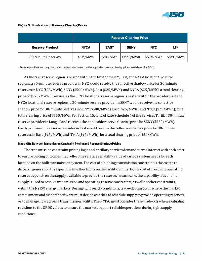
Figure 5: Illustration of Reserve Clearing Prices
*Reserve providers on Long Island are compensated based on the applicable reserve clearing prices established for SENY.
As the NYC reserve region is nested within the broader SENY, East, and NYCA locational reserve
regions, a 30-minute reserve provider in NYC would receive the collective shadow price for 30-minute
reserves in NYC ($25/MWh), SENY ($500/MWh), East ($25/MWh), and NYCA ($25/MWh); a total clearing
price of $575/MWh. Likewise, as the SENY locational reserve region is nested within the broader East and
NYCA locational reserve regions, a 30-minute reserve provider in SENY would receive the collective
shadow price for 30-minute reserves in SENY ($500/MWh), East ($25/MWh), and NYCA ($25/MWh); for a
total clearing price of $550/MWh. Per Section 15.4.4.2 of Rate Schedule 4 of the Services Tariff, a 30-minute
reserve provider in Long Island receives the applicable reserve clearing price for SENY ($550/MWh).
Lastly, a 30-minute reserve provider in East would receive the collective shadow price for 30-minute
reserves in East ($25/MWh) and NYCA ($25/MWh); for a total clearing price of $50/MWh.
Trade-Offs Between Transmission Constraint Pricing and Reserve Shortage Pricing
The transmission constraint pricing logic and ancillary services demand curves interact with each other
to ensure pricing outcomes that reflect the relative reliability value of various system needs for each
location on the bulk transmission system. The cost of a binding transmission constraint is the cost to re-
dispatch generation to respect the line flow limits on the facility. Similarly, the cost of procuring operating
reserve depends on the supply available to provide the reserve. In each case, the capability of available
supply is used to resolve transmission and operating reserve constraints, as well as other constraints,
within the NYISO energy markets. During tight supply conditions, trade-offs can occur where the market
commitment and dispatch software must decide whether to schedule supply to provide operating reserves
or to manage flow across a transmission facility. The NYISO must consider these trade-offs when evaluating
revisions to the ORDC values to ensure the markets support reliable operations during tight supply
conditions.
Reserve Clearing Price
Reserve Product NYCA EAST SENY NYC LI*
30-Minute Reserves $25/MWh $50/MWh $550/MWh $575/MWh $550/MWh
DRAFT PURPOSES ONLY Ancillary Services Shortage Pricing | 9
Neighboring ISO/RTO Demand Curve Levels
The neighboring markets administered by ISO-NE and PJM also use operating reserve demand curves
to price their respective reserve products.
ISO-NE currently procures four operating reserve products including:
■ Local 30-minute operating reserve with a $250/MWh shortage pricing value;
■ System 30-minute operating reserve where the minimum 30-minute requirement is priced at $1,000/MWh shortage pricing value. A quantity of 30-minute operating reserve beyond the minimum reserve requirement is also procured as “replacement reserve.” Replacement reserves are valued at a shortage cost of $250/MWh and do not cascade with other reserve shortage prices;
■ System 10-minute non-synchronized reserve with a $1,500/MWh shortage pricing value; and ■ System 10-minute spinning reserve with a $50/MWh shortage pricing value.
If all four reserve constraints were violated, the maximum reserve price would be $2,800/MWh. ISO-NE
assigns a value of $100/MWh to regulation service shortages.
PJM’s reserve requirements are calculated dynamically, based on the single largest generator
contingency. Currently, in its day-ahead market, PJM only secures the applicable 30-minute reserve
requirements. In its real-time market, PJM secures the applicable “primary reserve” requirements (total 10-
minute reserves) and “synchronous reserve” requirements (10-minute spinning reserves).
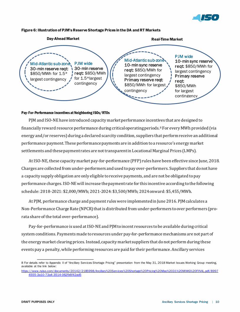
PJM’s current reserve shortage pricing includes a two-step demand curve. When reserves fall below the
dynamic requirement plus 190 MW, the shortage price is $300/MWh. Shortages in excess of this level are
valued at $850/MWh. In real-time, the maximum reserve price would be $1,700/MWh if the system were
short both primary and synchronous reserves. Regulation shortages are valued at $100/MWh in PJM. An
illustration of the cascading nature of PJM’s current reserve shortage prices and the products procured in
the day-ahead and real-time markets is shown in Figure 6 below.
In March 2019, PJM filed a proposal seeking to revise certain pricing values to better align shortage
pricing with the value of maintaining system reliability.7 The proposed changes filed by PJM remain
pending at FERC. PJM is also considering further enhancing its reserves demand curves with the probability
of loss of load and value of lost load concepts.
7 Docket No. EL19-58-000, PJM Interconnection, L.L.C., Enhanced Price Formation in Reserve Markets (March 29, 2019).
DRAFT PURPOSES ONLY Ancillary Services Shortage Pricing | 10
Figure 6: Illustration of PJM's Reserve Shortage Prices in the DA and RT Markets
Day-Ahead Market
Pay-For-Performance Incentives at Neighboring ISOs/RTOs
PJM and ISO-NE have introduced capacity market performance incentives that are designed to
financially reward resource performance during critical operating periods.8 For every MWh provided (via
energy and/or reserves) during a declared scarcity condition, suppliers that perform receive an additional
performance payment. These performance payments are in addition to a resource’s energy market
settlements and these payment rates are not transparent in Locational Marginal Prices (LMPs).
At ISO-NE, these capacity market pay-for-performance (PFP) rules have been effective since June, 2018.
Charges are collected from under-performers and used to pay over-performers. Suppliers that do not have
a capacity supply obligation are only eligible to receive payments, and are not be obligated to pay
performance charges. ISO-NE will increase the payment rate for this incentive according to the following
schedule: 2018-2021: $2,000/MWh; 2021-2024: $3,500/MWh; 2024 onward: $5,455/MWh.
At PJM, performance charge and payment rules were implemented in June 2016. PJM calculates a
Non-Performance Charge Rate (NPCR) that is distributed from under-performers to over performers (pro-
rata share of the total over-performance).
Pay-for-performance is used at ISO-NE and PJM to incent resources to be available during critical
system conditions. Payments made to resources under pay-for-performance mechanisms are not part of
the energy market clearing prices. Instead, capacity market suppliers that do not perform during these
events pay a penalty, while performing resources are paid for their performance. Ancillary services
8 For details refer to Appendix II of “Ancillary Services Shortage Pricing” presentation from the May 31, 2018 Market Issues Working Group meeting, available at the link below: https://www.nyiso.com/documents/20142/2185998/Ancillary%20Services%20Shortage%20Pricing%20May%2031%20MIWG%20FINAL.pdf/8997
4555-3a10-73a4-3514-062fb6f42ad5
Mid-Atlantic sub-zone 30-min reserve reqt: $850/MWh for 1.5* largest contingency
PJM wide 30-min reserve reqt: $850/MWh for 1.5*largest contingency
Mid-Atlantic sub-zone 10-min sync reserve reqt: $850/MWh for largest contingency Pr imary reserve reqt: $850/MWh for largest contingency
PJM wide 10-min sync reserve reqt: $850/MWh for largest contingency Pr imary reserve reqt: $850/MWh for largest contingency
Real-Time Market
DRAFT PURPOSES ONLY Ancillary Services Shortage Pricing | 11
shortage pricing performs a similar function in the NYISO markets. Reserve and regulation clearing prices
should rise as the grid approaches critical system conditions, and fall as grid conditions return to normal.
Pay-for-performance programs do not utilize real-time energy market prices to incent resources. Market-
based price signals and ancillary services shortage pricing enables the NYISO to incent resource
performance.
Historical Shortage Pricing Analysis The NYISO conducted an analysis of historical ancillary services shortage prices, as outlined in the
following sections. This analysis provides context for the shortage pricing that the NYISO experiences.
Shortages of NYCA 30-minute reserves are valuable to analyze in further detail, as the clearing price for
shortages of NYCA 30-minute reserves do not include the cascaded value of any other reserve products.
Frequency of NYCA 30-Minute Reserve Shortages
Shortages of NYCA 30-minute reserves were among the most frequent shortages observed over the
three-year historic period evaluated (July 2016 through September 2019). Further analysis was performed
to assess the applicable Shadow Prices during these shortages.
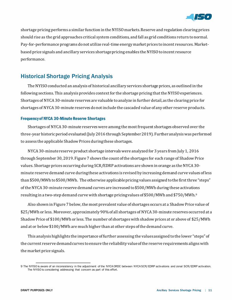
NYCA 30-minute reserve product shortage intervals were analyzed for 3 years from July 1, 2016
through September 30, 2019. Figure 7 shows the count of the shortages for each range of Shadow Price
values. Shortage prices occurring during SCR/EDRP activations are shown in orange as the NYCA 30-
minute reserve demand curve during these activations is revised by increasing demand curve values of less
than $500/MWh to $500/MWh. The otherwise applicable pricing values assigned to the first three “steps”
of the NYCA 30-minute reserve demand curves are increased to $500/MWh during these activations
resulting in a two-step demand curve with shortage pricing values of $500/MWh and $750/MWh.9
Also shown in Figure 7 below, the most prevalent value of shortages occurs at a Shadow Price value of
$25/MWh or less. Moreover, approximately 90% of all shortages of NYCA 30-minute reserves occurred at a
Shadow Price of $100/MWh or less. The number of shortages with shadow prices at or above of $25/MWh
and at or below $100/MWh are much higher than at other steps of the demand curve.
This analysis highlights the importance of further assessing the values assigned to the lower “steps” of
the current reserve demand curves to ensure the reliability value of the reserve requirements aligns with
the market price signals.
9 The NYISO is aware of an inconsistency in the adjustment of the NYCA ORDC between NYCA SCR/EDRP activations and zonal SCR/EDRP activation.
The NYISO is considering addressing that concern as part of this effort.
DRAFT PURPOSES ONLY Ancillary Services Shortage Pricing | 12
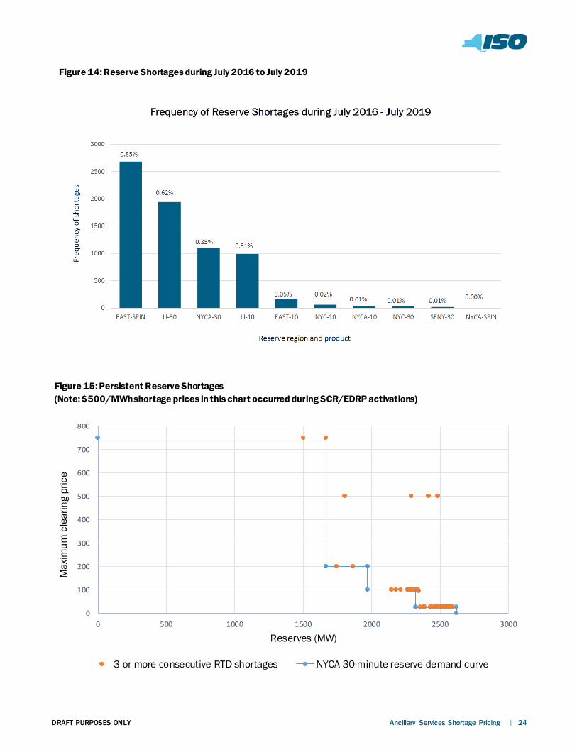
Persistent Reserve Shortage Analysis
Historic data from July 1, 2016 through August 31, 2019 was analyzed to assess the persistence of
reserve shortages in real-time. Persistent shortages could be indicative of a systematic concern with the
pricing values assigned to various levels of shortage.
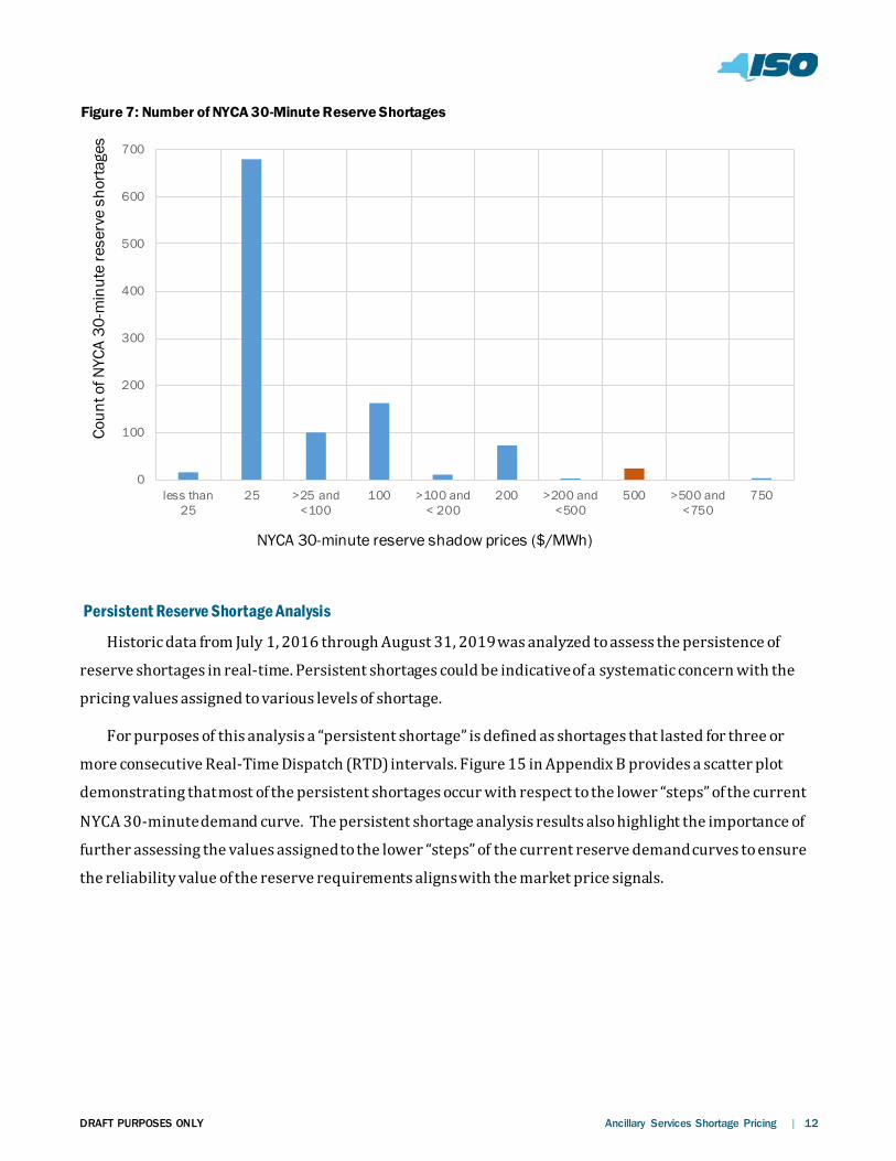
For purposes of this analysis a “persistent shortage” is defined as shortages that lasted for three or
more consecutive Real-Time Dispatch (RTD) intervals. Figure 15 in Appendix B provides a scatter plot
demonstrating that most of the persistent shortages occur with respect to the lower “steps” of the current
NYCA 30-minute demand curve. The persistent shortage analysis results also highlight the importance of
further assessing the values assigned to the lower “steps” of the current reserve demand curves to ensure
the reliability value of the reserve requirements aligns with the market price signals.
0
100
200
300
400
500
600
700
less than25
25 >25 and<100
100 >100 and< 200
200 >200 and<500
500 >500 and<750
750
Coun
t of N
YCA
30-m
inut
e re
serv
e sh
orta
ges
NYCA 30-minute reserve shadow prices ($/MWh)
Figure 7: Number of NYCA 30-Minute Reserve Shortages
DRAFT PURPOSES ONLY Ancillary Services Shortage Pricing | 13
Analysis of September 3, 2018 The MMU has previously highlighted the market outcomes from September 3, 2018 as an important
factor in assessing the need for potential changes to the current ancillary services shortage prices in New
York. This day is important because it provides an opportunity to assess how effectively the market prices
supported the actions taken by operators to maintain grid reliability when the system conditions were
tight not only in New York, but across a broader region.
This date was the first time that the pay-for-performance incentives were triggered in ISO-NE.
Resources that performed in ISO-NE had the chance to receive an additional $2,000/MWh performance
incentive payment during this event.10 This incentive payment is in excess of the prevailing energy and
reserve clearing prices.
System conditions in ISO-NE were very tight resulting from an under-forecast of load (2,500 MW
under-forecast) and an unexpected generation loss of 1,600 MW (in-day forced outage). The unexpected
generation loss accounted for 7% of ISO-NE’s peak load for that day. Further details regarding system
conditions and market outcomes from September 3, 2018 is provided in Appendix C.
Due to the operating conditions it was experiencing, ISO-NE cut certain exports to Long Island.
Shortages in the Real-Time Commitment (RTC) were analyzed to evaluate the RTC decisions to go short
reserves rather than commit or dispatch resources or keep the resources online. For this analysis, all the
time steps of each RTC run were analyzed during the time frame 14:00 through 22:00.
It was observed that RTC was in fact seeing reserve shortages in its forward horizon but decided to go
short of the product rather than commit and dispatch additional resources. These outcomes underscore the
importance of further assessing the current reserve shortage pricing levels to ensure that the reliability
value of the reserve procured matches market price signals and are consistent with operator actions during
stressed system conditions.
Emergency Energy Purchases from Ontario
As a result of its system needs, ISO-NE also made emergency energy purchases from New York on
September 3, 2018. To fulfill ISO-NE’s emergency purchase request, NYISO purchased emergency energy
from Ontario to supply to ISO-NE. Notably, during the time ISO-NE requested emergency assistance, NYISO
was experiencing a shortage of NYCA 30-minute reserves.
10 Notably, the value of this incentive payment rate is scheduled to increase over the coming years to a value of $5,455/MWh in 2024.
DRAFT PURPOSES ONLY Ancillary Services Shortage Pricing | 14
Upon analyzing the transactions available to RTC for the 17:00 to 18:00 timeframe, it was observed that
all of the economic transactions from Ontario were fully scheduled. In other words, all the imports that
were bid-in were fully scheduled or partially scheduled to match Ontario’s system and no exports were
bid-in.
Additional details regarding the assessment of the emergency energy purchases are provided in
Appendix C.
September 3, 2018 Day Rerun Analysis
The NYISO evaluated the potential impacts on the market outcomes from September 3, 2018 that could
have resulted from the use of higher shortage pricing values for the first three steps of the NYCA 30-minute
reserve demand curve. To conduct this assessment, the RTC with a timestamp of 16:30 was rerun in the
market software with a revised NYCA 30-minute reserve demand curve. This RTC run was selected because
it exhibited shortages of NYCA 30-minute reserves as part of its actual outcomes for September 3, 2018.
Additionally, the first RTC that would have seen imports from Cross-Sound Cable (CSC) cut would have
been the RTC that initialized at 16:00 and posted at 16:15. The selected case for the rerun was the RTC that
initialized at 16:15 and posted at 16:30, ensuring that the case included the curtailed exports from ISO-NE.
For purposes of the evaluation, the rerun was conducted using the following changes to the current
NYCA 30-minute reserve demand curve: (1) the $25/MWh NYCA reserve demand curve price was
increased to $50/MWh; (2) the $100/MWh demand curve price was increased to $300/MWh; and (3) the
$200 demand curve price was increased to $500/MWh.
The market simulation rerun with revised NYCA 30-minute reserve demand curve values exhibited an
increase in the amount of 30-minute reserve procured statewide. This is because reserve shortages were
partially avoided in the rerun, due to the higher demand curve values that were assigned to the reserve.
Shortages were primarily avoided by generator re-dispatch (i.e., decreasing the output of reserve qualified
generators to provide reserve, while increasing the output of other generators in order to provide energy).
For example, overall generator schedule changes for the 16:45 look-ahead interval from the September
3, 2018 RTC rerun are shown in Figure 18 in Appendix C. The schedule changes show that some generator
schedules were reduced when the original case is compared to the rerun case, while other generator
schedules were increased. Figure 17 in Appendix C further shows increases in reserve schedules in the
rerun. The results from this limited rerun demonstrate the potential ability for increases in the current
reserve demand curve values to provide for an increase in the level of reserves available during critical
operating periods.
DRAFT PURPOSES ONLY Ancillary Services Shortage Pricing | 15
Understanding Value of Lost Load
VOLL Background
Value of Lost Load (VOLL) can be defined as the cost (in $/MWh) imposed by involuntary load
curtailment. Generally, VOLL will vary by customer and time. That is, the VOLL for a homeowner in upstate
New York can be different than the VOLL for a homeowner on Long Island. Likewise, VOLL for the same
homeowner is different during overnight hours than during daytime or early morning hours. Considering
various VOLL methodologies and values can, however, be useful when considering potential adjustments to
the NYISO’s ORDCs used in shortage pricing.
For the purpose of reserves valuation, VOLL can be defined as the value that 1 MW reserve increment
has in preventing 1 MW of load shed. In other words, as operating reserves can help prevent the need to
shed load, in this approach, operating reserve shortage pricing reflects the VOLL as the available reserves
approach 0 MW. The MMU has recommended using VOLL as a consideration in establishing reserve
demand curve values in New York.11 In response, the NYISO has assessed illustrative VOLL-based reserve
demand curve structures for NYCA 30-minute and 10-minute total reserves. These illustrative curves were
developed as another mechanism for evaluating the current reserve shortage pricing values used in the
NYISO-administered markets.
VOLL Based Shortage Pricing Consideration
Under the VOLL approach for shortage pricing, the maximum price level on the ORDC is set at VOLL.
It is accompanied with a probability, often referred as Loss of Load Probability (LOLP), which is the
probability of reserves falling below a predefined minimum reserves level or zero (if there are no
predefined reserves level). The MMU has suggested that reserve shortage pricing values should consider
the VOLL multiplied by LOLP.12
𝑉𝑉𝑉𝑉𝑉𝑉𝑉𝑉𝑉𝑉 𝑜𝑜𝑜𝑜 𝑅𝑅𝑉𝑉𝑅𝑅𝑉𝑉𝑅𝑅𝑅𝑅𝑉𝑉 (𝑅𝑅) = 𝑉𝑉𝑉𝑉𝑉𝑉𝑉𝑉 ∗ 𝑉𝑉𝑉𝑉𝑉𝑉𝐿𝐿 (𝑅𝑅)
where, R = Reserve Level
The value of reserves using this approach depends upon the cost imposed by involuntary load
curtailment discounted by the probability of losing reserves at a given reserve level.
11 Potomac Economics. 2018 State of the Market Report for the New York ISO Markets. May 2019. 12 See footnote no. 11
DRAFT PURPOSES ONLY Ancillary Services Shortage Pricing | 16
Further detail on the consideration of VOLL in other wholesale markets is provided in Appendix D.
VOLL Estimation for New York
VOLL depends on multiple parameters, including but not limited to, customer type, time of load loss,
duration of load loss, availability of advance warning mechanisms, and measures a customer may have
already implemented to help mitigate the impacts of potential load loss. All these factors make the
estimation of a single value of VOLL very difficult.
A major limitation in using VOLL for shortage pricing is the uncertainty around its value and estimation
methods. There have been multiple studies in the past based on different estimation methods, calculating
different values for VOLL both in the U.S. and abroad. Three broad methods for VOLL estimations identified
in a study by London Economics International (LEI)13 include:
1. Customer Surveys: Customer surveys are designed to estimate a customer’s willingness to pay to avoid load shedding, which is taken as a proxy for VOLL. Customer surveys are expensive to conduct and their results can be affected by survey design and customer’s intentions.
2. Macroeconomic Analysis: In this method, broad economic indicators are taken as a proxy for VOLL. Economy wide VOLL is estimated as the ratio of annual Gross Domestic Product (GDP) and annual electricity consumption. This is a very high-level approach and has multiple limitations, such as not accounting for the flexibility of demand across customers, supply chain impacts associated with an outage, time and duration of outages. For customers, VOLL can also be calculated as the ratio of electricity bill to consumption. This generally tends to result in low estimates of VOLL, as the electricity price likely does not fully reflect the actual value associated with its use from the end-user’s perspective.
3. Case study of an actual outage event: This method aims to estimate the value of lost load by estimating the loss associated with an actual outage event. Data for such estimation is difficult to obtain and the results may not be universally applicable to other outage events.
Based on the literature review of estimation methods, two methods have been used to derive an
estimate of potential VOLL for New York. Using a macroeconomic method, average VOLL across all
customer types was estimated at $11,000/MWh. Using the Interruption Cost Estimation (ICE) 14 tool based
on prior VOLL estimation for the certain U.S. utilities, the average VOLL for New York across all customer
types was estimated at $60,000/MWh. Further detail about these estimation methodologies is provided in
Appendix D. These estimates were used in conjunction with estimated LOLP values to derive illustrative
VOLL-based ORDCs for NYCA 30-minute and 10-minute total reserves. This was intended to provide an
additional analytical tool for assessing the current shortage pricing values used in the NYISO-administered
13 London Economics International LLC. Estimating the Value of Lost Load. June 17, 2013 14 ICE Calculator. Available at: https://icecalculator.com/home
DRAFT PURPOSES ONLY Ancillary Services Shortage Pricing | 17
markets.
Loss of Load Probability
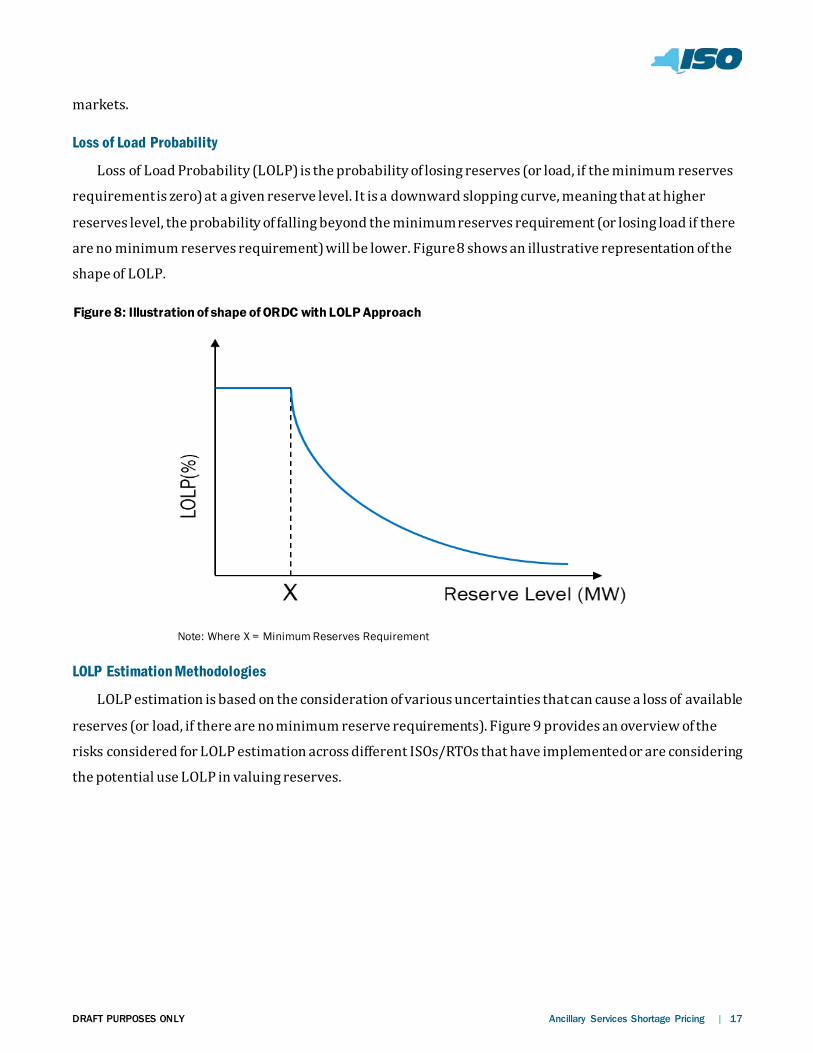
Loss of Load Probability (LOLP) is the probability of losing reserves (or load, if the minimum reserves
requirement is zero) at a given reserve level. It is a downward slopping curve, meaning that at higher
reserves level, the probability of falling beyond the minimum reserves requirement (or losing load if there
are no minimum reserves requirement) will be lower. Figure 8 shows an illustrative representation of the
shape of LOLP.
Note: Where X = Minimum Reserves Requirement
LOLP Estimation Methodologies
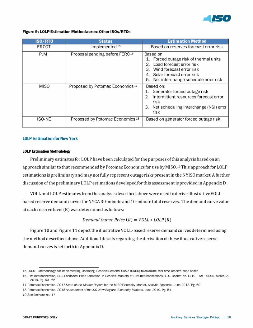
LOLP estimation is based on the consideration of various uncertainties that can cause a loss of available
reserves (or load, if there are no minimum reserve requirements). Figure 9 provides an overview of the
risks considered for LOLP estimation across different ISOs/RTOs that have implemented or are considering
the potential use LOLP in valuing reserves.
Figure 8: Illustration of shape of ORDC with LOLP Approach
DRAFT PURPOSES ONLY Ancillary Services Shortage Pricing | 18
Figure 9: LOLP Estimation Method across Other ISOs/RTOs
ISO/RTO Status Estimation Method ERCOT Implemented 15 Based on reserves forecast error risk PJM Proposal pending before FERC16 Based on
1. Forced outage risk of thermal units 2. Load forecast error risk 3. Wind forecast error risk 4. Solar forecast error risk 5. Net interchange schedule error risk
MISO Proposed by Potomac Economics 17 Based on: 1. Generator forced outage risk 2. Intermittent resources forecast error
risk 3. Net scheduling interchange (NSI) error
risk ISO-NE Proposed by Potomac Economics 18 Based on generator forced outage risk
LOLP Estimation for New York
LOLP Estimation Methodology
Preliminary estimates for LOLP have been calculated for the purposes of this analysis based on an
approach similar to that recommended by Potomac Economics for use by MISO.19 This approach for LOLP
estimations is preliminary and may not fully represent outage risks present in the NYISO market. A further
discussion of the preliminary LOLP estimations developed for this assessment is provided in Appendix D .
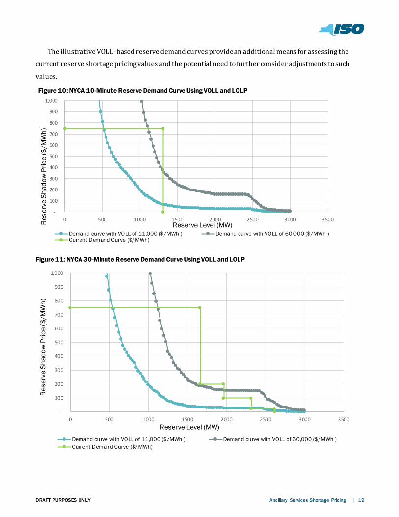
VOLL and LOLP estimates from the analysis described above were used to derive illustrative VOLL-
based reserve demand curves for NYCA 30-minute and 10-minute total reserves. The demand curve value
at each reserve level (R) was determined as follows:
𝐷𝐷𝑉𝑉𝐷𝐷𝑉𝑉𝐷𝐷𝐷𝐷 𝐶𝐶𝑉𝑉𝑅𝑅𝑅𝑅𝑉𝑉 𝐿𝐿𝑅𝑅𝑃𝑃𝑃𝑃𝑉𝑉 (𝑅𝑅) = 𝑉𝑉𝑉𝑉𝑉𝑉𝑉𝑉 ∗ 𝑉𝑉𝑉𝑉𝑉𝑉𝐿𝐿(𝑅𝑅)
Figure 10 and Figure 11 depict the illustrative VOLL-based reserve demand curves determined using
the method described above. Additional details regarding the derivation of these illustrative reserve
demand curves is set forth in Appendix D.
15 ERCOT. Methodology for Implementing Operating Reserve Demand Curve (ORDC) to calculate real-time reserve price adder. 16 PJM Interconnection, LLC. Enhanced Price Formation in Reserve Markets of PJM Interconnections, LLC. Docket No. EL19 – 58 – 0000. March 29,
2019. Pg. 53 - 66 17 Potomac Economics. 2017 State of the Market Report for the MISO Electricity Market, Analytic Appendix. June 2018. Pg. 60 18 Potomac Economics. 2018 Assessment of the ISO New England Electricity Markets. June 2019. Pg. 51 19 See footnote no. 17
DRAFT PURPOSES ONLY Ancillary Services Shortage Pricing | 19
The illustrative VOLL-based reserve demand curves provide an additional means for assessing the
current reserve shortage pricing values and the potential need to further consider adjustments to such
values.
-
100
200
300
400
500
600
700
800
900
1,000
0 500 1000 1500 2000 2500 3000 3500Res
erve
Sha
dow
Pric
e ($
/MW
h)
Reserve Level (MW)Demand curve with VOLL of 11,000 ($/MWh ) Demand curve with VOLL of 60,000 ($/MWh )Current Demand Curve ($/MWh)
Figure 10: NYCA 10-Minute Reserve Demand Curve Using VOLL and LOLP
-
100
200
300
400
500
600
700
800
900
1,000
0 500 1000 1500 2000 2500 3000 3500
Res
erve
Sha
dow
Pric
e ($
/MW
h)
Reserve Level (MW)
Demand curve with VOLL of 11,000 ($/MWh ) Demand curve with VOLL of 60,000 ($/MWh )Current Demand Curve ($/MWh)
Figure 11: NYCA 30-Minute Reserve Demand Curve Using VOLL and LOLP
DRAFT PURPOSES ONLY Ancillary Services Shortage Pricing | 20
Conclusion Ancillary services are becoming increasingly important for supporting system reliability as the grid
transitions to include more weather-dependent renewable resources. Appropriately valuing ancillary
services, especially during stressed operating conditions, supports achieving reliability through markets.
The price signals for these services are important for signaling the need for investment in maintaining and
adding new resources capable of providing the resource capabilities needed to reliably operate the system.
The results of this assessment demonstrate that the majority of current NYCA 30-minute reserve shortages
occur at Shadow Price values of $100/MWh or less. The analysis also determined that shortages of NYCA
30-minute reserve shortages persisting for three or more RTD intervals are also most likely to occur at
such lower pricing levels.
The MMU has also noted that pay-for-performance capacity market rules in neighboring ISOs/RTOs
present potential concerns that the current reserve shortage pricing values in New York may not be
adequate to ensure reserve capability in New York is maintained during stressed system conditions that
extend beyond New York to include such neighboring regions. Analysis of market outcomes and events
from September 3, 2018 (i.e., a date when pay-for-performance incentives were activated in ISO-NE and
both New York and ISO-NE experienced stressed operating conditions), highlights this potential concern.
During the stressed conditions, the current reserve shortage pricing levels resulted in RTC incurring
reserve shortages rather than committing and/or dispatching additional resources to allow for
procurement of the needed reserves. A rerun of the RTC market software demonstrated that adjustments
to the current reserve shortage pricing levels would have facilitated additional reserve procurements
during these stressed operating conditions.
Separately, the illustrative pricing curves from the VOLL analysis could be useful when considering
potential adjustments to the current shortage pricing values and/or whether additional pricing “steps” may
provide for more predictable and stable price signals.
Based on the results of the analysis conducted, the NYISO recommends further collaboration with
stakeholders to assess potential changes to the current reserve shortage prices values used in the NYISO-
administered markets. Specifically, the NYISO and its stakeholders should consider increasing lower
reserve demand curve pricing values to help avoid frequent shortages, and improve the consistency of
market price signals with the reliability value of these ancillary services products.
DRAFT PURPOSES ONLY Ancillary Services Shortage Pricing | 21
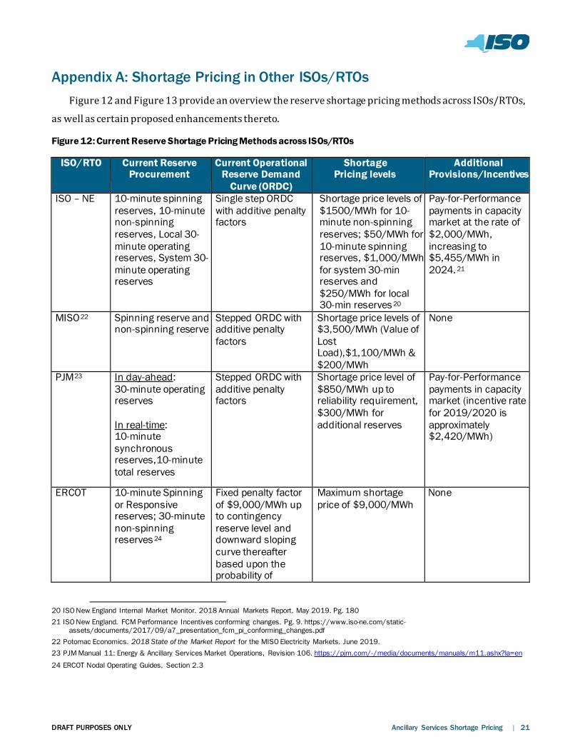
Appendix A: Shortage Pricing in Other ISOs/RTOs Figure 12 and Figure 13 provide an overview the reserve shortage pricing methods across ISOs/RTOs,
as well as certain proposed enhancements thereto.
Figure 12: Current Reserve Shortage Pricing Methods across ISOs/RTOs
ISO/RTO Current Reserve Procurement
Current Operational Reserve Demand
Curve (ORDC)
Shortage Pricing levels
Additional Provisions/Incentives
ISO – NE 10-minute spinning reserves, 10-minute non-spinning reserves, Local 30-minute operating reserves, System 30-minute operating reserves
Single step ORDC with additive penalty factors
Shortage price levels of $1500/MWh for 10-minute non-spinning reserves; $50/MWh for 10-minute spinning reserves, $1,000/MWh for system 30-min reserves and $250/MWh for local 30-min reserves 20
Pay-for-Performance payments in capacity market at the rate of $2,000/MWh, increasing to $5,455/MWh in 2024. 21
MISO22 Spinning reserve and non-spinning reserve
Stepped ORDC with additive penalty factors
Shortage price levels of $3,500/MWh (Value of Lost Load),$1,100/MWh & $200/MWh
None
PJM23 In day-ahead: 30-minute operating reserves In real-time: 10-minute synchronous reserves,10-minute total reserves
Stepped ORDC with additive penalty factors
Shortage price level of $850/MWh up to reliability requirement, $300/MWh for additional reserves
Pay-for-Performance payments in capacity market (incentive rate for 2019/2020 is approximately $2,420/MWh)
ERCOT
10-minute Spinning or Responsive reserves; 30-minute non-spinning reserves 24
Fixed penalty factor of $9,000/MWh up to contingency reserve level and downward sloping curve thereafter based upon the probability of
Maximum shortage price of $9,000/MWh
None
20 ISO New England Internal Market Monitor. 2018 Annual Markets Report. May 2019. Pg. 180 21 ISO New England. FCM Performance Incentives conforming changes. Pg. 9. https://www.iso-ne.com/static-
assets/documents/2017/09/a7_presentation_fcm_pi_conforming_changes.pdf 22 Potomac Economics. 2018 State of the Market Report for the MISO Electricity Markets. June 2019. 23 PJM Manual 11: Energy & Ancillary Services Market Operations, Revision 106. https://pjm.com/-/media/documents/manuals/m11.ashx?la=en 24 ERCOT Nodal Operating Guides, Section 2.3
DRAFT PURPOSES ONLY Ancillary Services Shortage Pricing | 22
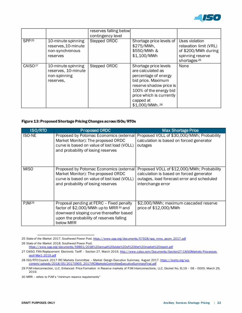
reserves falling below contingency level
SPP25 10-minute spinning reserves,10-minute non-synchronous reserves
Stepped ORDC
Shortage price levels of $275/MWh, $550/MWh & $1,100/MWh
Uses violation relaxation limit (VRL) of $200/MWh during spinning reserve shortages 26
CAISO27 10-minute spinning reserves, 10-minute non-spinning reserves,
Stepped ORDC Shortage price levels are calculated as percentage of energy bid price. Maximum reserve shadow price is 100% of the energy bid price which is currently capped at $1,000/MWh. 28
None
Figure 13: Proposed Shortage Pricing Changes across ISOs/RTOs
ISO/RTO Proposed ORDC Max Shortage Price ISO-NE Proposed by Potomac Economics (external
Market Monitor): The proposed ORDC curve is based on value of lost load (VOLL) and probability of losing reserves
Proposed VOLL of $30,000/MWh; Probability calculation is based on forced generator outages
MISO Proposed by Potomac Economics (external Market Monitor): The proposed ORDC curve is based on value of lost load (VOLL) and probability of losing reserves
Proposed VOLL of $12,000/MWh; Probability calculation is based on forced generator outages, load forecast error and scheduled interchange error
PJM29 Proposal pending at FERC – Fixed penalty factor of $2,000/MWh up to MRR 30 and downward sloping curve thereafter based upon the probability of reserves falling below MRR
$2,000/MWh; maximum cascaded reserve price of $12,000/MWh
25 State of the Market 2017. Southwest Power Pool. https://www.spp.org/documents/57928/spp_mmu_asom_2017.pdf 26 State of the Market 2018. Southwest Power Pool.
https://www.spp.org/documents/59861/2018%20annual%20state%20of%20the%20market%20report.pdf 27 CAISO. Fifth Replacement Electronic Tariff – Section 27. March 2019. http://www.caiso.com/Documents/Section27-CAISOMarkets-Processes-
asof-Mar1-2019.pdf 28 ISO/RTO Council. 2017 IRC Markets Committee – Market Design Executive Summary. August 2017. https://isorto.org/wp-
content/uploads/2018/05/20170905_2017IRCMarketsCommitteeExecutiveSummaryFinal.pdf 29 PJM Interconnection, LLC. Enhanced Price Formation in Reserve markets of PJM Interconnections, LLC. Docket No. EL19 – 58 – 0000. March 29,
2019. 30 MRR – refers to PJM’s “minimum reserve requirements”
DRAFT PURPOSES ONLY Ancillary Services Shortage Pricing | 23
CAISO Under current market rules, the maximum reserve shadow price is 100% of the energy bid price. A proposal pending at FERC31 seeks to modify the maximum energy bid price to $2,000/MWh.
Propose a bid cap of $2,000/MWh, which would revise the maximum reserve shadow price to $2,000/MWh.
Appendix B: Historical Shortage Pricing Analysis
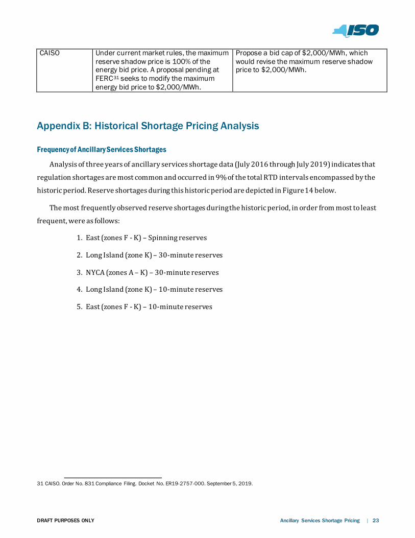
Frequency of Ancillary Services Shortages
Analysis of three years of ancillary services shortage data (July 2016 through July 2019) indicates that
regulation shortages are most common and occurred in 9% of the total RTD intervals encompassed by the
historic period. Reserve shortages during this historic period are depicted in Figure 14 below.
The most frequently observed reserve shortages during the historic period, in order from most to least
frequent, were as follows:
1. East (zones F - K) – Spinning reserves
2. Long Island (zone K) – 30-minute reserves
3. NYCA (zones A – K) – 30-minute reserves
4. Long Island (zone K) – 10-minute reserves
5. East (zones F - K) – 10-minute reserves
31 CAISO. Order No. 831 Compliance Filing. Docket No. ER19-2757-000. September 5, 2019.
DRAFT PURPOSES ONLY Ancillary Services Shortage Pricing | 24
Figure 14: Reserve Shortages during July 2016 to July 2019
0
100
200
300
400
500
600
700
800
0 500 1000 1500 2000 2500 3000
Max
imum
cle
arin
g pr
ice
Reserves (MW)
3 or more consecutive RTD shortages NYCA 30-minute reserve demand curve
Figure 15: Persistent Reserve Shortages (Note: $500/MWh shortage prices in this chart occurred during SCR/EDRP activations)
DRAFT PURPOSES ONLY Ancillary Services Shortage Pricing | 25
Appendix C: Analysis of September 3, 2018
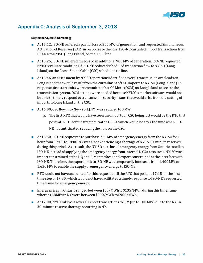
September 3, 2018 Chronology
■ At 15:12, ISO-NE suffered a partial loss of 300 MW of generation, and requested Simultaneous Activation of Reserves (SAR) in response to the loss. ISO-NE curtailed import transactions from ISO-NE to NYISO (Long Island) on the 1385 line.
■ At 15:25, ISO-NE suffered the loss of an additional 900 MW of generation. ISO-NE requested NYISO evaluate conditions if ISO-NE reduced scheduled transaction flow to NYISO (Long Island) on the Cross-Sound Cable (CSC) scheduled tie line.
■ At 15:46, an assessment by NYISO operations identified several transmission overloads on Long Island that would result from the curtailment of CSC imports to NYISO (Long Island). In response, fast start units were committed Out-Of-Merit (OOM) on Long Island to secure the transmission system. OOM actions were needed because NYISO’s market software would not be able to timely respond to transmission security issues that would arise from the cutting of imports to Long Island on the CSC.
■ At 16:00, CSC flow into New York(NY) was reduced to 0 MW. a. The first RTC that would have seen the imports on CSC being lost would be the RTC that
posts at 16:15 for the first interval of 16:30, which would be after the time when ISO-
NE had anticipated reducing the flow on the CSC.
■ At 16:50, ISO-NE requested to purchase 250 MW of emergency energy from the NYISO for 1 hour from 17:00 to 18:00. NY was also experiencing a shortage of NYCA 30-minute reserves during this period. As a result, the NYISO purchased emergency energy from Ontario to sell to ISO-NE instead of supplying the emergency energy from internal NYCA resources. NYISO was import constrained at the HQ and PJM interfaces and export constrained at the interface with ISO-NE. Therefore, the export limit to ISO-NE was temporarily increased from 1,400 MW to 1,650 MW to enable the supply of emergency energy to ISO-NE.
■ RTC would not have accounted for this request until the RTC that posts at 17:15 for the first time step of 17:30, which would not have facilitated a timely response to ISO-NE’s requested timeframe for emergency energy.
■ Energy prices in Ontario ranged between $50/MWh to $135/MWh during this timeframe, whereas LBMPs in NY were between $200/MWh to $900/MWh.
■ At 17:00, NYISO also cut several export transactions to PJM (up to 100 MW) due to the NYCA 30-minute reserve shortage occurring in NY.
DRAFT PURPOSES ONLY Ancillary Services Shortage Pricing | 26
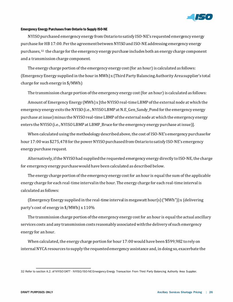
Emergency Energy Purchases from Ontario to Supply ISO-NE
NYISO purchased emergency energy from Ontario to satisfy ISO-NE’s requested emergency energy
purchase for HB 17:00. Per the agreement between NYISO and ISO-NE addressing emergency energy
purchases,32 the charge for the emergency energy purchase includes both an energy charge component
and a transmission charge component.
The energy charge portion of the emergency energy cost (for an hour) is calculated as follows:
(Emergency Energy supplied in the hour in MWh) x (Third Party Balancing Authority Area supplier’s total
charge for such energy in $/MWh)
The transmission charge portion of the emergency energy cost (for an hour) is calculated as follows:
Amount of Emergency Energy (MWh) x [the NYISO real-time LBMP of the external node at which the
emergency energy exits the NYISO (i.e., NYISO LBMP at N.E_Gen_Sandy_Pond for the emergency energy
purchase at issue) minus the NYISO real-time LBMP of the external node at which the emergency energy
enters the NYISO (i.e., NYISO LBMP at LBMP_Bruce for the emergency energy purchase at issue)].
When calculated using the methodology described above, the cost of ISO-NE’s emergency purchase for
hour 17:00 was $275,478 for the power NYISO purchased from Ontario to satisfy ISO-NE’s emergency
energy purchase request.
Alternatively, if the NYISO had supplied the requested emergency energy directly to ISO-NE, the charge
for emergency energy purchase would have been calculated as described below.
The energy charge portion of the emergency energy cost for an hour is equal the sum of the applicable
energy charge for each real-time interval in the hour. The energy charge for each real-time interval is
calculated as follows:
(Emergency Energy supplied in the real-time interval in megawatt hour(s) (“MWh”)) x (delivering
party’s cost of energy in $/MWh) x 110%
The transmission charge portion of the emergency energy cost for an hour is equal the actual ancillary
services costs and any transmission costs reasonably associated with the delivery of such emergency
energy for an hour.
When calculated, the energy charge portion for hour 17:00 would have been $599,982 to rely on
internal NYCA resources to supply the requested emergency assistance and, in doing so, exacerbate the
32 Refer to section A.2. of NYISO OATT - NYISO/ISO-NE Emergency Energy Transaction From Third Party Balancing Authority Area Supplier.
DRAFT PURPOSES ONLY Ancillary Services Shortage Pricing | 27
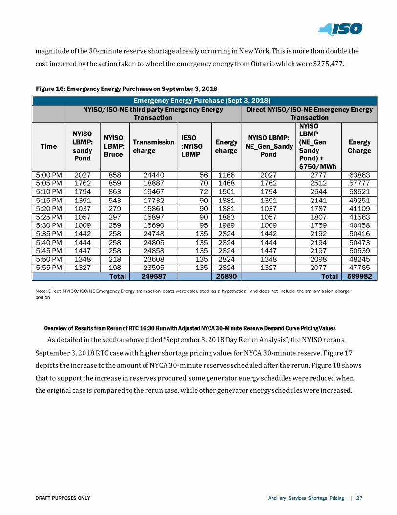
magnitude of the 30-minute reserve shortage already occurring in New York. This is more than double the
cost incurred by the action taken to wheel the emergency energy from Ontario which were $275,477.
Emergency Energy Purchase (Sept 3, 2018)
NYISO/ISO-NE third party Emergency Energy
Transaction Direct NYISO/ISO-NE Emergency Energy
Transaction
Time
NYISO LBMP: sandy Pond
NYISO LBMP: Bruce
Transmission charge
IESO :NYISO LBMP
Energy charge
NYISO LBMP: NE_Gen_Sandy
Pond
NYISO LBMP (NE_Gen Sandy Pond) + $750/MWh
Energy Charge
5:00 PM 2027 858 24440 56 1166 2027 2777 63863 5:05 PM 1762 859 18887 70 1468 1762 2512 57777 5:10 PM 1794 863 19467 72 1501 1794 2544 58521 5:15 PM 1391 543 17732 90 1881 1391 2141 49251 5:20 PM 1037 279 15861 90 1881 1037 1787 41109 5:25 PM 1057 297 15897 90 1883 1057 1807 41563 5:30 PM 1009 259 15690 95 1989 1009 1759 40458 5:35 PM 1442 258 24748 135 2824 1442 2192 50416 5:40 PM 1444 258 24805 135 2824 1444 2194 50473 5:45 PM 1447 258 24858 135 2824 1447 2197 50539 5:50 PM 1348 218 23608 135 2824 1348 2098 48245 5:55 PM 1327 198 23595 135 2824 1327 2077 47765
Total 249587 25890 Total 599982
Note: Direct NYISO/ISO-NE Emergency Energy transaction costs were calculated as a hypothetical and does not include the transmission charge portion
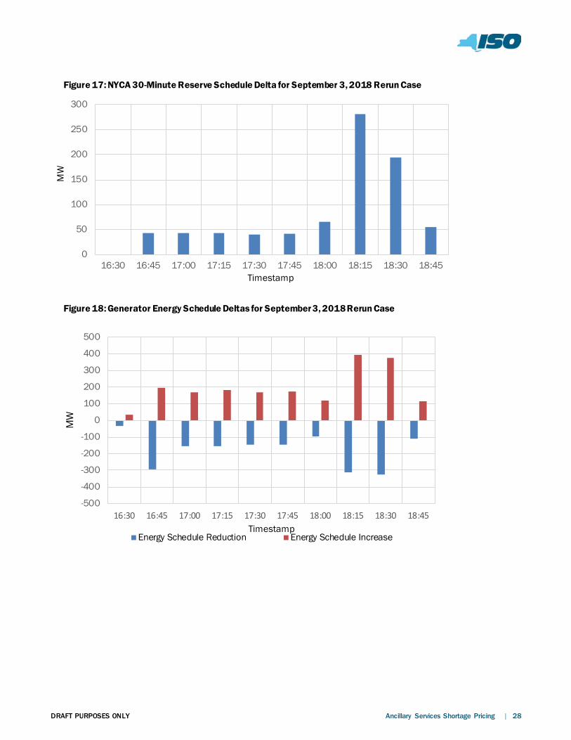
Overview of Results from Rerun of RTC 16:30 Run with Adjusted NYCA 30-Minute Reserve Demand Curve Pricing Values
As detailed in the section above titled “September 3, 2018 Day Rerun Analysis”, the NYISO reran a
September 3, 2018 RTC case with higher shortage pricing values for NYCA 30-minute reserve. Figure 17
depicts the increase to the amount of NYCA 30-minute reserves scheduled after the rerun. Figure 18 shows
that to support the increase in reserves procured, some generator energy schedules were reduced when
the original case is compared to the rerun case, while other generator energy schedules were increased.
Figure 16: Emergency Energy Purchases on September 3, 2018
DRAFT PURPOSES ONLY Ancillary Services Shortage Pricing | 28
Figure 17: NYCA 30-Minute Reserve Schedule Delta for September 3, 2018 Rerun Case
-500
-400
-300
-200
-100
0
100
200
300
400
500
16:30 16:45 17:00 17:15 17:30 17:45 18:00 18:15 18:30 18:45
MW
TimestampEnergy Schedule Reduction Energy Schedule Increase
Figure 18: Generator Energy Schedule Deltas for September 3, 2018 Rerun Case
0
50
100
150
200
250
300
16:30 16:45 17:00 17:15 17:30 17:45 18:00 18:15 18:30 18:45
MW
Timestamp
DRAFT PURPOSES ONLY Ancillary Services Shortage Pricing | 29
Appendix D: Value of Lost Load
VOLL Background
Estimating VOLL is complicated by the fact that it depends on multiple factors, including customer type,
time of load loss, duration of load loss, availability of advance warning mechanisms, and measures a
customer may have already implemented to help mitigate the impacts of potential load loss.
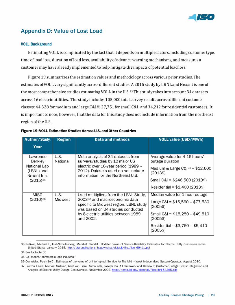
Figure 19 summarizes the estimation values and methodology across various prior studies. The
estimates of VOLL vary significantly across different studies. A 2015 study by LBNL and Nexant is one of
the most comprehensive studies estimating VOLL in the U.S.33 This study takes into account 34 datasets
across 16 electric utilities. The study includes 105,000 total survey results across different customer
classes: 44,328 for medium and large C&I35; 27,751 for small C&I; and 34,212 for residential customers. It
is important to note; however, that the data for this study does not include information from the northeast
region of the U.S.
Figure 19: VOLL Estimation Studies Across U.S. and Other Countries
Author/Study,
Year
Region Data and methods VOLL value (USD/MWh)
Lawrence Berkley
National Lab (LBNL) and Nexant Inc.
(2015)34
U.S. National
Meta-analysis of 34 datasets from surveys/studies by 10 major US electric over 16-year period (1989 – 2012). Datasets used do not include information for the Northeast U.S.
Average value for 4-16 hours’ outage duration
Medium & Large C&I 35 = $12,600 (2013$)
Small C&I = $246,500 (2013$)
Residential = $1,400 (2013$)
MISO (2010)36
U.S. Midwest
Used multipliers from the LBNL Study, 200337 and macroeconomic data specific to Midwest region. LBNL study was based on 24 studies conducted by 8 electric utilities between 1989 and 2002.
Median value for 1-hour outage
Large C&I = $15,560 – $77,530 (2005$)
Small C&I = $15,250 – $49,510 (2005$)
Residential = $3,760 – $5,410 (2005$)
33 Sullivan, Michael J., Josh Schellenberg, Marshall Blundell. Updated Value of Service Reliability Estimates for Electric Utility Customers in the
United States. January 2015. http://eta-publications.lbl.gov/sites/default/files/lbnl-6941e.pdf 34 See footnote 33 35 C&I means “commercial and industrial” 36 Centelella, Paul (SAIC). Estimates of the value of Uninterrupted Service for The Mid – West Independent System Operator. August 2010. 37 Lawton, Leora, Michael Sullivan, Kent Van Liere, Aaron Kalz, Joseph Eto. A Framework and Review of Customer Outage Costs: Integration and
Analysis of Electric Utility Outage Cost Surveys. November 2003. https://emp.lbl.gov/sites/all/files/lbnl-54365.pdf
DRAFT PURPOSES ONLY Ancillary Services Shortage Pricing | 30
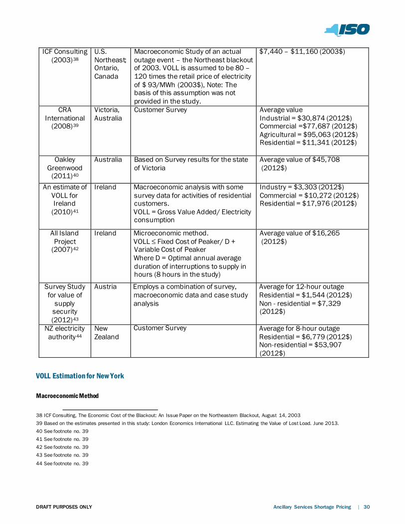
ICF Consulting (2003)38
U.S. Northeast; Ontario, Canada
Macroeconomic Study of an actual outage event – the Northeast blackout of 2003. VOLL is assumed to be 80 – 120 times the retail price of electricity of $ 93/MWh (2003$), Note: The basis of this assumption was not provided in the study.
$7,440 – $11,160 (2003$)
CRA International
(2008)39
Victoria, Australia
Customer Survey Average value Industrial = $30,874 (2012$) Commercial =$77,687 (2012$) Agricultural = $95,063 (2012$) Residential = $11,341 (2012$)
Oakley Greenwood
(2011)40
Australia Based on Survey results for the state of Victoria
Average value of $45,708 (2012$)
An estimate of VOLL for Ireland
(2010)41
Ireland Macroeconomic analysis with some survey data for activities of residential customers. VOLL = Gross Value Added/ Electricity consumption
Industry = $3,303 (2012$) Commercial = $10,272 (2012$) Residential = $17,976 (2012$)
All Island Project
(2007)42
Ireland Microeconomic method. VOLL ≤ Fixed Cost of Peaker/ D + Variable Cost of Peaker Where D = Optimal annual average duration of interruptions to supply in hours (8 hours in the study)
Average value of $16,265 (2012$)
Survey Study for value of
supply security (2012)43
Austria Employs a combination of survey, macroeconomic data and case study analysis
Average for 12-hour outage Residential = $1,544 (2012$) Non - residential = $7,329 (2012$)
NZ electricity authority44
New Zealand
Customer Survey Average for 8-hour outage Residential = $6,779 (2012$) Non-residential = $53,907 (2012$)
VOLL Estimation for New York
Macroeconomic Method
38 ICF Consulting, The Economic Cost of the Blackout: An Issue Paper on the Northeastern Blackout, August 14, 2003 39 Based on the estimates presented in this study: London Economics International LLC. Estimating the Value of Lost Load. June 2013. 40 See footnote no. 39 41 See footnote no. 39 42 See footnote no. 39 43 See footnote no. 39 44 See footnote no. 39
DRAFT PURPOSES ONLY Ancillary Services Shortage Pricing | 31
One macroeconomic method of estimating VOLL is to calculate VOLL as the ratio of GDP and electricity
consumption.13 Using the value of New York GDP of $1,600 billion and New York electricity consumption of
145 million MWh in 2017, VOLL is estimated to be $ 11,000/MWh in 2017 U.S. dollars.45
Using Interruption Cost Estimation tool
The Interruption Cost Estimation (ICE) tool is an electric reliability planning tool developed by
Lawrence Berkeley National Lab and Nexant Inc. It is based on a study on service reliability estimates for
electric utility customers in the United States that uses the data from 34 customer surveys conducted by 10
major US electric utilities over 16-year period (1989 – 2012).46 This tool can be used to calculate an
estimated average interruption cost (in $ per unserved kWh) for a state based on user inputs.47 Using the
ICE calculator, the average VOLL for New York is estimated at $60,000/MWh across all customer types.
VOLL Approach for Reserve Shortage Pricing and its Adoption across Other ISOs/RTOs
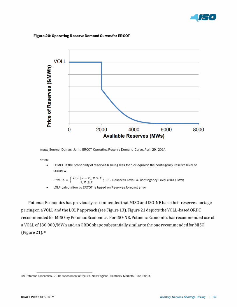
Currently only ERCOT has implemented an ORDC based on a VOLL and LOLP approach. Figure 20
shows the ORDC for ERCOT. ERCOT values up to 2,000 MW of reserves at VOLL. In excess of 2,000 MW,
reserves are valued at a lower value depending on various factors.
45 New York GDP and electricity consumption for 2017 was taken from Bureau of Economic Analysis (BEA) and U.S. Energy Information
Administration, respectively. 46 See footnote 33 47 User inputs include number of residential and non-residential customers; Reliability index values for SAIFI (System Average Interruption Frequency
Index) and CAIDI (Customer Average Interruption Duration Index)
DRAFT PURPOSES ONLY Ancillary Services Shortage Pricing | 32
Potomac Economics has previously recommended that MISO and ISO-NE base their reserve shortage
pricing on a VOLL and the LOLP approach (see Figure 13). Figure 21 depicts the VOLL-based ORDC
recommended for MISO by Potomac Economics. For ISO-NE, Potomac Economics has recommended use of
a VOLL of $30,000/MWh and an ORDC shape substantially similar to the one recommended for MISO
(Figure 21).48
48 Potomac Economics. 2018 Assessment of the ISO New England Electricity Markets. June 2019.
Image Source: Dumas, John. ERCOT Operating Reserve Demand Curve. April 29, 2014. Notes:
• PBMCL is the probability of reserves R being less than or equal to the contingency reserve level of
2000MW.
𝐿𝐿𝑃𝑃𝑃𝑃𝐶𝐶𝑉𝑉 = �𝑉𝑉𝑉𝑉𝑉𝑉𝐿𝐿(𝑅𝑅 − 𝑋𝑋),𝑅𝑅 > 𝑋𝑋1,𝑅𝑅 ≤ 𝑋𝑋 ; R – Reserves Level, X- Contingency Level (2000 MW)
• LOLP calculation by ERCOT is based on Reserves forecast error
Figure 20: Operating Reserve Demand Curves for ERCOT

DRAFT PURPOSES ONLY Ancillary Services Shortage Pricing | 33
LOLP Estimation for New York
LOLP Estimation Methodology
Estimates for LOLP were calculated based on an approach recommended by Potomac Economics for
MISO.49 LOLP estimation is done for NYCA 10-minute total and NYCA 30-minute reserves using a Monte
Carlo simulation to simulate possible outages due to different risks that can result in a loss of reserves in
real-time. Three types of risks are considered:
1. Generator Forced Outage Risk: This represents the risk of losing reserves due to
generator(s) outages at any instant of time.
2. Load and Intermittent Resource Forecast Error Risk: This represents the risk of losing
49 See footnote no. 17
Image Source: “2018 Energy Conference Energy Information Administration”, Presentation by Dr. David B. Patton, Potomac Economics. June 4, 2018 Notes: IMM for MISO proposed a VOLL of $ 12,000 / MWh, the slope of the proposed curve is based on probability of losing load at that reserve level. Probability of losing load is estimated using a Monte Carlo simulation incorporating generator forced outage risk, intermittent resource forecast error and net imports changes.
Figure 21: Proposed ORDC for MISO
DRAFT PURPOSES ONLY Ancillary Services Shortage Pricing | 34
reserves due to differences between forecasted and actual load levels and wind output.
3. Desired Net Interchange (DNI) Error Risk: This represents the risk of losing reserves due
to differences between RTC and RTD Net Interchange schedules.
Generator Forced Outage Risk
The calculation approach for potential loss of reserves/load caused by generator forced outage risk
involves estimating the possibility of generators experiencing an outage at any instant of time. Such
estimation is based on technology specific factors that help in determining the outage risks faced by
different types of generating resources, excluding wind and solar. Occurrence of outages across available
generators is randomized based on the technology specific factors. The technology specific factors for
generators are:
■ Participation factor (PF): PF for a generation technology type can be calculated as the ratio of
the sum of the online capacity of that type to the sum of the installed capacity of that type across
all hours of a specified historical period.
■ Mean Service Time to Unplanned Outage (MSTUO): MSTUO for a generation technology
represents the average number of hours between two unplanned outages. This value can be
calculated as the ratio of service hours to the number of unplanned outages for a generation
technology type.
For purposes of this assessment, the values of these factors for different generation technologies were
assumed to be similar to the values recommended by Potomac Economics for MISO. In addition to the
factors above, another factor — Outage Recovery Period (ORP)50 has been considered in the analysis.
Based on these three factors discussed above, the value of [1− 𝑉𝑉^ (𝐿𝐿𝑃𝑃 ∗𝑉𝑉𝑅𝑅𝐿𝐿) 𝑃𝑃𝑀𝑀𝑀𝑀𝑀𝑀𝑉𝑉]⁄ is calculated.
For each iteration of the Monte Carlo simulation, a random number between 0 and 1 is assigned to all generators. If this random number is less than the value of [1 −𝑉𝑉^ (𝐿𝐿𝑃𝑃 ∗ 𝑉𝑉𝑅𝑅𝐿𝐿) 𝑃𝑃𝑀𝑀𝑀𝑀𝑀𝑀𝑉𝑉]⁄ for that
generator, the generator is assumed to experience an outage. Total outage MW due to generator outage
risks for each iteration is the sum of outages across all generators in that iteration calculated using the
method described here. Simulating this potential outage value for large number of iterations provides a
reasonable estimate of expected outage MW at any instant resulting from the potential for generator forced
outages.
50 Outage Recovery Period is no. of hours needed to fully respond to applicable supply side contingencies. For MISO, Potomac Economics’ proposal
utilized a value of 2 hours. This assessment uses this same value.
DRAFT PURPOSES ONLY Ancillary Services Shortage Pricing | 35
Weather-dependent resources like solar and wind generation resources are not included in this
calculation. Risk associated with those technologies are included in the load and intermittent resources
forecast error risk which is discussed in the following section.
Load and Intermittent Resources Forecast Error Risk
The calculation for the potential loss of reserves/load and intermittent resource forecast error risk is
based on the distribution of this error from a three-year historical dataset (May 2016 through April 2019).
Net Load Forecast Error includes both load and intermittent resource forecast risk and is calculated as:
𝑁𝑁𝑉𝑉𝑁𝑁 𝑉𝑉𝑜𝑜𝑉𝑉𝐷𝐷 𝑃𝑃𝑜𝑜𝑅𝑅𝑉𝑉𝑃𝑃𝑉𝑉𝑅𝑅𝑁𝑁 𝐸𝐸𝑅𝑅𝑅𝑅𝑜𝑜𝑅𝑅 = (𝐴𝐴𝑃𝑃𝑁𝑁𝑉𝑉𝑉𝑉𝑉𝑉 𝑉𝑉𝑜𝑜𝑉𝑉𝐷𝐷 −𝑃𝑃𝑜𝑜𝑅𝑅𝑉𝑉𝑃𝑃𝑉𝑉𝑅𝑅𝑁𝑁 𝑉𝑉𝑜𝑜𝑉𝑉𝐷𝐷) − (𝐴𝐴𝑃𝑃𝑁𝑁𝑉𝑉𝑉𝑉𝑉𝑉 𝑊𝑊𝑃𝑃𝐷𝐷𝐷𝐷 −𝑃𝑃𝑜𝑜𝑅𝑅𝑉𝑉𝑃𝑃𝑉𝑉𝑅𝑅𝑁𝑁 𝑊𝑊𝑃𝑃𝐷𝐷𝐷𝐷)
Mean and standard deviation from the net load forecast error calculation were used to create a
cumulative normal distribution function for this historically observed error. Outage risk (MW) due to net
load forecast error in each iteration of the Monte Carlo simulation is calculated as the maximum of zero and
the inverse of the cumulative normal distribution function from the distribution at a random distribution
probability. The distribution probability is varied randomly for all iterations in the simulation to capture
the range of possible risk of loss (MW) that can occur due to this error. Net Load Forecast Error in the 30-
minute timeframe is used for estimating LOLP for NYCA 30-minute reserves and Net Load Forecast Error in
the 10-minute timeframe is used for estimating LOLP for NYCA 10-minute reserves.
Desired Net Interchange Error Risk
The calculation for the potential loss of reserves/load due to Desired Net Interchange (DNI) error risk
uses a similar methodology as calculation for load and intermittent resource forecast error risk. This error
risk is based on the distribution of DNI error from a three-year historical dataset (May 2016 through April
2019). The DNI error is calculated as:
𝐷𝐷𝑁𝑁𝐷𝐷 𝐸𝐸𝑅𝑅𝑅𝑅𝑜𝑜𝑅𝑅 = 𝑅𝑅𝑀𝑀𝐶𝐶 𝑁𝑁𝑉𝑉𝑁𝑁 𝐷𝐷𝐷𝐷𝑁𝑁𝑉𝑉𝑅𝑅𝑃𝑃ℎ𝑉𝑉𝐷𝐷𝑎𝑎𝑉𝑉− 𝑅𝑅𝑀𝑀𝐷𝐷 𝑁𝑁𝑉𝑉𝑁𝑁 𝐷𝐷𝐷𝐷𝑁𝑁𝑉𝑉𝑅𝑅𝑃𝑃ℎ𝑉𝑉𝐷𝐷𝑎𝑎𝑉𝑉
RTC (Real-Time Commitment) schedules every 15-minutes. There are three Real-Time Dispatch (RTD)
timestamps that correspond to one RTC timestamp. Once RTC schedules interchange, it takes RTD some
time to ramp up/down to follow the RTC schedule. To account for this systematic lag between RTC and
RTD, the second RTD timestamp corresponding to the RTC timestamp is used to calculate the DNI error.
Mean and standard deviation from the DNI error calculation were used to create a cumulative normal
distribution function for this historically observed error. Outage risk (MW) due to DNI error in each
iteration of the Monte Carlo simulation is calculated as the maximum of zero and the inverse of the
cumulative normal distribution function from the distribution at a random distribution probability. The
distribution probability was varied randomly for all iterations in the simulation to capture the range of
DRAFT PURPOSES ONLY Ancillary Services Shortage Pricing | 36
possible risk of loss (MW) that can occur due to this error.
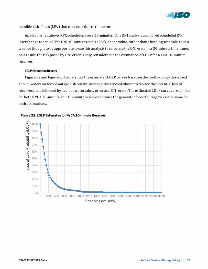
As established above, RTC schedules every 15-minutes. This DNI analysis compared scheduled RTC
interchange to actual. The DNI 30-minutes out is a look-ahead value, rather than a binding schedule, thus it
was not thought to be appropriate to use this analysis to calculate the DNI error in a 30-minute timeframe.
As a result, the risk posed by DNI error is only considered in the estimation of LOLP for NYCA 10-minute
reserves.
LOLP Estimation Results
Figure 22 and Figure 23 below show the estimated LOLP curves based on the methodology described
above. Generator forced outage risk constitutes the primary contributor to risk for the potential loss of
reserves/load followed by net load uncertainty error and DNI error. The estimated LOLP curves are similar
for both NYCA 30-minute and 10-minute reserves because the generator forced outage risk is the same for
both estimations.
0%
10%
20%
30%
40%
50%
60%
70%
80%
90%
100%
0 200 400 600 800 1000 1200 1400 1600 1800 2000 2200 2400 2600 2800 3000
Loss
of L
oad
Prob
abili
ty (L
OLP
)
Reserve Level (MW)
Figure 22: LOLP Estimates for NYCA 10-minute Reserves
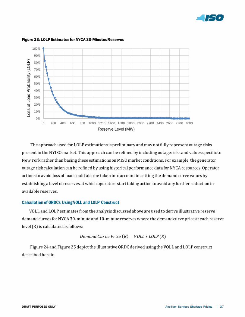
DRAFT PURPOSES ONLY Ancillary Services Shortage Pricing | 37
The approach used for LOLP estimations is preliminary and may not fully represent outage risks
present in the NYISO market. This approach can be refined by including outage risks and values specific to
New York rather than basing these estimations on MISO market conditions. For example, the generator
outage risk calculation can be refined by using historical performance data for NYCA resources. Operator
actions to avoid loss of load could also be taken into account in setting the demand curve values by
establishing a level of reserves at which operators start taking action to avoid any further reduction in
available reserves.
Calculation of ORDCs Using VOLL and LOLP Construct
VOLL and LOLP estimates from the analysis discussed above are used to derive illustrative reserve
demand curves for NYCA 30-minute and 10-minute reserves where the demand curve price at each reserve
level (R) is calculated as follows:
𝐷𝐷𝑉𝑉𝐷𝐷𝑉𝑉𝐷𝐷𝐷𝐷 𝐶𝐶𝑉𝑉𝑅𝑅𝑅𝑅𝑉𝑉 𝐿𝐿𝑅𝑅𝑃𝑃𝑃𝑃𝑉𝑉 (𝑅𝑅) = 𝑉𝑉𝑉𝑉𝑉𝑉𝑉𝑉 ∗ 𝑉𝑉𝑉𝑉𝑉𝑉𝐿𝐿(𝑅𝑅)
Figure 24 and Figure 25 depict the illustrative ORDC derived using the VOLL and LOLP construct
described herein.
0%
10%
20%
30%
40%
50%
60%
70%
80%
90%
100%
0 200 400 600 800 1000 1200 1400 1600 1800 2000 2200 2400 2600 2800 3000
Loss
of L
oad
Prob
abili
ty (L
OLP
)
Reserve Level (MW)
Figure 23: LOLP Estimates for NYCA 30-Minutes Reserves
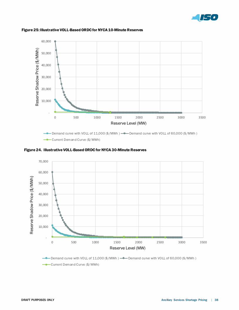
DRAFT PURPOSES ONLY Ancillary Services Shortage Pricing | 38
-
10,000
20,000
30,000
40,000
50,000
60,000
0 500 1000 1500 2000 2500 3000 3500
Res
erve
Sha
dow
Pric
e ($
/MW
h)
Reserve Level (MW)
Demand curve with VOLL of 11,000 ($/MWh ) Demand curve with VOLL of 60,000 ($/MWh )
Current Demand Curve ($/MWh)
Figure 25: Illustrative VOLL-Based ORDC for NYCA 10-Minute Reserves
-
10,000
20,000
30,000
40,000
50,000
60,000
70,000
0 500 1000 1500 2000 2500 3000 3500
Res
erve
Sha
dow
Pric
e ($
/MW
h)
Reserve Level (MW)
Demand curve with VOLL of 11,000 ($/MWh ) Demand curve with VOLL of 60,000 ($/MWh )
Current Demand Curve ($/MWh)
Figure 24. Illustrative VOLL-Based ORDC for NYCA 30-Minute Reserves