analytical solutions for contaminant diffusion in …orca.cf.ac.uk/8277/1/li.pdf · analytical...

Dow

nloa

ded

from

asc

elib

rary

.org

by

Car

diff

Uni

vers

ity o

n 02

/25/

14. C

opyr

ight

ASC

E. F

or p

erso

nal u

se o

nly;

all

righ

ts r

eser

ved.

Analytical Solutions for Contaminant Diffusionin Double-Layered Porous Media

Yu-Chao Li1 and Peter John Cleall2

Abstract: Analytical solutions for conservative solute diffusion in one-dimensional double-layered porous media are presented in thispaper. These solutions are applicable to various combinations of fixed solute concentration and zero-flux boundary conditions �BC�applied at each end of a finite one-dimensional domain and can consider arbitrary initial solute concentration distributions throughout themedia. Several analytical solutions based on several initial and BCs are presented based on typical contaminant transport problems foundin geoenvironmental engineering including �1� leachate diffusion in a compacted clay liner �CCL� and an underlying stratum; �2�contaminant removal from soil layers; and �3� contaminant diffusion in a capping layer and underlying contaminated sediments. Theanalytical solutions are verified against numerical solutions from a finite-element method based model. Problems related to leachatetransport in a CCL and an underlying stratum of a landfill and contaminant transport through a capping layer over contaminated sedimentsare then investigated, and the suitable definition of the average degree of diffusion is considered.

DOI: 10.1061/�ASCE�GT.1943-5606.0000365

CE Database subject headings: Analytical techniques; Containment; Diffusion; Layered systems; Porous media.

Author keywords: Analytical techniques; Containment; Diffusion; Layered systems; Porous media.

Introduction

Contaminant transport analysis is undertaken when consideringgeoenvironmental problems such as the evaluation and design ofengineered/natural containment barrier systems for waste disposaland the containment and remediation of existing contaminatedsoils �Sharma and Reddy 2004�. In particular, contaminant diffu-sion analysis in porous media is of great importance in that dif-fusion often dominates the contaminant transport processes inengineered barriers, natural containment systems, and geologicalsoil/rock media �Shackelford and Lee 2005�.

One-dimensional diffusion of solute in a semiinfinite or finitehomogeneous porous medium can be analyzed via use of analyti-cal solutions for diffusion in solids �Crank 1956; Carslaw andJaeger 1959�. Contaminant transport in a system consisting of twosoil layers, whose soil and transport properties are quite differentfrom each other, is often observed in geoenvironmental engineer-ing problems. For example, leachate transfer through a compactedclay liner �CCL� and an underlying stratum in landfills �Roweet al. 2004� and contaminant diffusion in capping layers overcontaminated sediments �Palermo et al. 1998b; Lampert and

1Lecturer, MOE Key Laboratory of Soft Soils and GeoenvironmentalEngineering, Department of Civil Engineering, Zhejiang Univ., Hang-zhou 310058, China; formerly, Research Associate, GeoenvironmentalResearch Centre, Cardiff School of Engineering, Cardiff Univ., CardiffCF24 3AA, Wales, U.K. E-mail: [email protected]

2Lecturer, Geoenvironmental Research Centre, Cardiff School of En-gineering, Cardiff Univ., Cardiff CF24 3AA, Wales, U.K. �correspondingauthor�. E-mail: [email protected]

Note. This manuscript was submitted on April 15, 2009; approved onApril 6, 2010; published online on April 10, 2010. Discussion periodopen until April 1, 2011; separate discussions must be submitted forindividual papers. This paper is part of the Journal of Geotechnical andGeoenvironmental Engineering, Vol. 136, No. 11, November 1, 2010.
©ASCE, ISSN 1090-0241/2010/11-1542–1554/$25.00.
1542 / JOURNAL OF GEOTECHNICAL AND GEOENVIRONMENTAL ENGIN

J. Geotech. Geoenviron. Eng.

Reible 2009� are often considered. These two examples are illus-trated in Fig. 1. The range of initial and boundary conditions�BCs� of many solutions is limited and is not suitable for manypractical contaminant diffusion problems. Some work has beendone on solving the diffusion or advection-dispersion equation ofsolute transports in two- or multilayered porous media using theLaplace transform method �Leij et al. 1991; Leij and van Genu-chten 1995�, the integral transform method �Liu et al. 1998�, andan approach combining the Laplace transformation method andbinomial theorem �Liu and Ball 1998�. Also, an analytical solu-tion for contaminant diffusion through multilayered system waspresented by Chen et al. �2009�; however, only scenarios with afixed top BC are considered as contaminant diffusion in landfillliners is the main focus of their work. The form of the solutionsconsidering multilayered system above �Chen et al. 2009; Leijet al. 1991; Leij and van Genuchten 1995; Liu and Ball 1998; Liuet al. 1998� while able to yield valuable insights into the mecha-nisms occurring is relatively complex and is not readily amenableto simple implementation.

This paper presents analytical solutions for conservative solute�in terms of mass� diffusion in one-dimensional double-layeredporous media subjected to arbitrary initial and BCs. The term“conservative solute” is used here to mean that no loss in mass ofthe solute species occurs during transport as opposed to indicatinga nonreactive solute. In fact, the solute is considered to be reac-tive via consideration of reversible, linear, and instantaneoussorption by the use of a retardation factor. This work is inspiredby the analogy between Terzaghi’s governing equation for con-solidation and Fick’s governing equation for diffusion presentedby Shackelford and Lee �2005�. The governing equations of sol-ute diffusion are solved following the approach of Lee et al.�1992� and Xie �1994� who considered consolidation in double-layered soils. The novelty of the solutions presented herein is bothin terms of the simplicity of the solutions relative to Laplacetransform approaches and the wider range of BCs that are consid-
ered. In contrast to Chen et al. �2009�, the number of layers is
EERING © ASCE / NOVEMBER 2010

2010.136:1542-1554.

Dow

nloa

ded

from

asc

elib

rary

.org

by

Car

diff

Uni

vers

ity o

n 02

/25/

14. C

opyr

ight

ASC

E. F

or p

erso

nal u

se o

nly;

all

righ

ts r

eser

ved.

restricted to 2; this restriction has the advantage of the resultingeigenvalued function being considerably less complex. Severalanalytical solutions subjected to a series of initial and BCs arepresented based on typical contaminant transport problems foundin geoenvironmental engineering. The analytical solutions areverified against numerical solutions by consideration of a hypo-thetical diffusion problem in a double-layered system and appliedto analyze both leachate transport in a CCL of a landfill and anunderlying stratum and contaminant transport in capped contami-nated sediments.

Theory

Problem Formulation

A porous medium consisting of two individual homogeneous lay-ers is considered, as illustrated in Fig. 2. A coordinate system �z�,whose positive direction is downward, is adopted, and the top ofthe upper layer is chosen as the origin of z. Each layer has its ownconstant effective diffusion coefficient �Di

��, retardation factor�Rdi�, and porosity �ni�. The subscript i represents the layer withi=1 corresponding to the upper layer and i=2 to the lower layer.

Fig. 1. Examples of contaminant diffusion in double-layered soils:�a� contaminant transport in a compacted clay landfill liner and anunderlying stratum; �b� contaminant diffusion through a cappinglayer over contaminated sediments

Fig. 2. Schematic representation of generalized domain for solutediffusion in a double-layered porous medium

Table 1. BCs for Double-Layered Systems Considered

Boundary Fixed concentrat

Top of layered system c1 �z=0

Bottom of layered system c2 �z=H

JOURNAL OF GEOTECHNICAL AND GEOE


The thicknesses of the upper layer and the lower layer are h1 andh2, respectively, and the total thickness H is h1+h2.

The effective diffusion coefficient is defined as the product ofthe apparent tortuosity factor �a and the aqueous diffusion coef-ficient for the solutes D0, i.e., D�=�aD0 �Freeze and Cherry 1979;Shackelford and Daniel 1991�. A linear reversible sorption iso-therm �Freeze and Cherry 1979� is considered such that the retar-dation factor can be written as Rdi=1+�iKdi /ni, where �i=bulkdry density of soil and Kdi=distribution coefficient. The govern-ing equation of solute diffusion in each layer �Shackelford andDaniel 1991� can be expressed as follows:

Rdi

�ci

�t= Di

��2ci

�z2 �i = 1,2� �1�

where t represents time and ci=solute concentration in the porewater of the ith layer.

The initial condition for the problem considered can be ex-pressed as

ci�t=0 = ci,t=0�z� �i = 1,2� �2�

where ci,t=0�z�=arbitrary function for the initial solute concentra-tion distribution in the ith soil layer. Several combinations of BCsare considered, as shown in Table 1, where cz=0�t� and cz=H�t�=time-dependent functions for the boundary solute concentrationat the top and bottom, respectively.

Solute concentration continuity and flux continuity are satis-fied at the interface between layers as follows:

c1�z=h1= c2�z=h1

�3a�

�n1D1��c1

�z�

z=h1

= �n2D2��c2

�z�

z=h1

�3b�

Following Shackelford and Lee �2005�, the relative amount ofsolute removed or gained in the two layers at any elapsed timecan be represented by the average degree of diffusion, Uc�t�, as

Uc�t� =M�0� − M�t�M�0� − M��

�4�

where M�t�=solute mass per unit area within the double-layeredsystem at time t and can be expressed by

M�t� = n1Rd1�0

h1

c1�z,t�dz + n2Rd2�h1

H

c2�z,t�dz �5�

The definition of the average degree of diffusion in Eq. �4� issimilar to the average degree of consolidation in Terzaghi’s theoryof consolidation �Terzaghi 1943�. However, the solute mass insoil, rather than the solute mass in pore water as used by Chenet al. �2009�, is considered in Eq. �4�. This difference in definitionof average degree of diffusion is discussed later in the “Applica-tions” section.

The diffusive solute mass flux in soil, Jc, can be written inaccordance with Fick’s first law for diffusion in soil as follows�Shackelford 1991; Shackelford and Lee 2005�:

irichlet� BC Zero-flux �von Neumann� BC

� �c1 /�z �z=0=0

t� �c2 /�z �z=H=0

ion �D

=cz=0�t=cz=H�

NVIRONMENTAL ENGINEERING © ASCE / NOVEMBER 2010 / 1543

2010.136:1542-1554.

Dow

nloa

ded

from

asc

elib

rary

.org

by

Car

diff

Uni

vers

ity o

n 02

/25/

14. C

opyr

ight

ASC

E. F

or p

erso

nal u

se o

nly;

all

righ

ts r

eser

ved.

Jc�z,t� = − niDi��ci�z,t�

�z�6�

Therefore, Jc may be obtained at any spatial or temporal locationvia substitution of the spatial derivative of the solute concentra-tion from the analytical solution.

Analytical Solutions

Analytical solutions for the governing equations, i.e., Eq. �1�,subjected to the initial condition, i.e., Eq. �2�, and the BCs inTable 1 and Eq. �3� are presented in this section. These are devel-oped following the approach proposed by Lee et al. �1992� andXie �1994� who considered the problem of linear elastic small-strain consolidation in double-layered soils. Although Fick’s gov-erning equation for diffusion is analogous to Terzaghi’s governingequation for consolidation �Shackelford and Lee 2005�, the fluxcontinuity condition at the interface of layers is different from thatof consolidation as a result of both its porosity dependence, i.e.,Eq. �3b�, and being based on Fick’s first law for diffusion versusDarcy’s law for consolidation.

The following dimensionless parameters for the soil and trans-port properties are defined to simplify the formulations of thesolutions:

� =D2

�

D1�

; � =Rd2

Rd1; � =

n2

n1; � =

h2

h1�7�

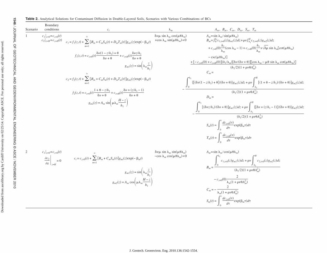
Fixed Surface - Zero-Flux Base ScenarioA scenario with a fixed, time-dependent concentration BC at thetop and a zero-flux BC at the bottom �i.e., fixed surface - zero-fluxbase scenario�, as given in Table 1, is considered in this section. Asolution for consolidation of a clay layer with free-draining BCsat both the top and bottom boundaries can be expressed as thesum of an infinite series of the product of a coefficient, a sinu-soidal function, and an exponential function, representing the ini-tial excess pore water pressure, depth, and elapsed time,respectively �Terzaghi 1943�. Following the form of the solutionsfor such consolidation problems presented by Terzaghi �1943�and Lee et al. �1992�, the solution for the scenario considered canbe written as follows:

ci�z,t� = cz=0�t� + �m=1

�

�Bm + CmSm�t��gmi�z�exp�− �mt� �8a�

gm1�z� = sin�m

z

h1 �8b�

gm2�z� = Am cos�m

H − z

h1 �8c�

where Am, Bm, Cm, �m, �m, and =coefficients to be determinedand Sm�t�=function with respect to time t and to be determined�which is introduced due to the term of the time-dependent con-centration BC at the top, i.e., cz=0�t��. Note that the functionSm�t�=0 if the fixed concentration BC is time independent.

The types of the trigonometric functions in Eqs. �8b� and �8c�are chosen according to the BCs applied at the top and the bottomof the system, respectively, with a sine function chosen for thefixed BC and a cosine function chosen for zero-flux BCs. Thevalue of the series function term in Eq. �8a� equals to zero at the
top �that is, z=0� using Eq. �8b� and the value of the term of the


series function’s derivative with respect to z in Eq. �8a� equals tozero at the bottom �that is, z=H� using Eq. �8c�. Consequently,the BCs at both the top and the bottom for the scenario consideredhere can be satisfied by the solution form of Eqs. �8a�–�8c�.

Substitution of Eqs. �8a�–�8c� into Eqs. �3a� and �3b�, i.e., toconsider continuity at the interface between the layers, yields

Am = sin �m/cos��m� �9�

�� sin �m sin��m� − cos �m cos��m� = 0 �10�

where Eq. �10� =eigenvalued function of �m. Further substitutionof Eqs. �8a� and �8b� into Eq. �1�, to consider the solute diffusionwithin the upper layer, yields

�m =D1

�

Rd1

�m2

h12 �11�

Sm�t� =�0

t dcz=0��d�

exp��m��d� �12�

�m=1

�

Cmgm1 = − 1 �13�

Similarly, substitution of Eqs. �8a� and �8c� into Eq. �1�, to con-sider the solute diffusion within the lower layer, yields

= ��/� �14�

�m=1

�

Cmgm2 = − 1 �15�

Finally, substitution of Eqs. �8a�–�8c� into Eq. �2�, to consider theinitial conditions, yields

ci,z=0�0� + �m=1

�

Bmgmi�z� = ci,t=0�z� �i = 1,2� �16�

Using the following orthogonal relations:

�0

h1

gm1�z�gn1�z�dz + ��h1

H

gm2�z�gn2�z�dz

= � 0 m � n

1

2h1�1 + ��Am

2 � m = n �17�

the following formulations for Bm and Cm based on Eqs. �13� and�15�–�17� can be obtained:

Bm = 2

�0

h1

c1,t=0�z�gm1�z�dz + ��h1

H

c2,t=0�z�gm2�z�dz

h1�1 + ��Am2 �

− cz=0�0�2

�m�1 + ��Am2 �

�18�

Cm = −2

�m�1 + ��Am2 �

�19�

The integral terms in Eq. �18� can be written explicitly if theinitial concentration function, ci,t=0�z�, has a simple form, such asa unique function; otherwise numerical integration techniques
�Chapra and Canale 2006� can be employed to solve the integral.

2010.136:1542-1554.

Dow

nloa

ded

from

asc

elib

rary

.org

by

Car

diff

Uni

vers

ity o

n 02

/25/

14. C

opyr

ight

ASC

E. F

or p

erso

nal u

se o

nly;

all

righ

ts r

eser

ved.

The analytical solution presented in this section is summarized inTable 2 as Scenario 2.

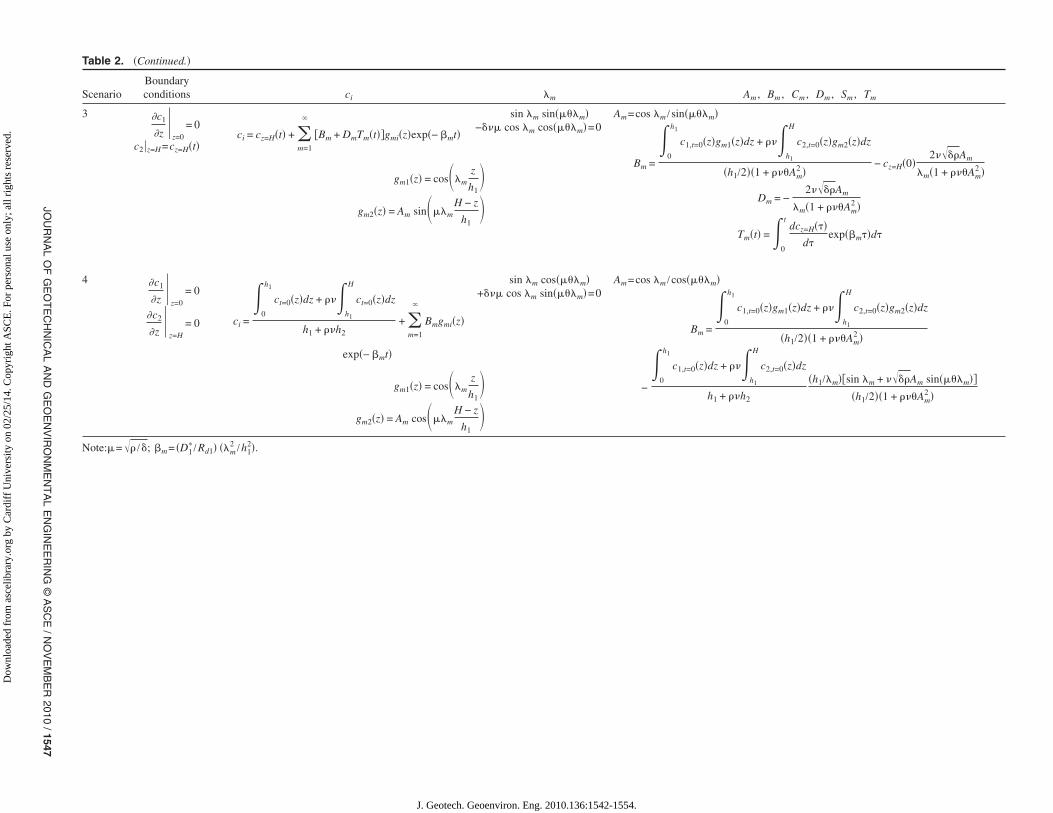
Other Boundary ScenariosThree other scenarios can be considered based on the other pos-sible combinations of different BCs at the top and the bottom ofthe system, as indicated in Table 2. Similar solutions to that forthe fixed surface and zero-flux base scenario can be establishedfor these three scenarios and are also detailed in Table 2. Sinefunctions again are adopted in the expressions of gm1�z� andgm2�z� for the fixed concentration BC, whereas cosine functionsare adopted for the zero-flux BCs. The unknown coefficients andfunctions can be obtained following the procedure presented forthe fixed surface-zero-flux base scenario and are also listed inTable 2.

The dichotomy technique, recommended by Xie �1994�, isadopted to solve the type of eigenvalue function of �m presentedin the analytical solutions. However, simple formulations of �m

can be obtained if ��=1, that is, ��=1, as follows:

�m = �m

1 + ��Scenarios 1 and 4�

�2m − 1�2�1 + ��

�Scenarios 2 and 3� �20�

With various combinations of initial and BCs, the analytical so-lutions presented above can be utilized to analyze many typicalcases for solute diffusion problems existing in geoenvironmentalengineering. A number of possible cases are considered herein,and the solutions are listed in Table 3. These solutions can be usedto consider the following solute transport problems:1. Leachate diffusion in a CCL and an underlying stratum

�Cases A and D�;2. Contaminant removal from soil layers �Cases B and E�; and3. Contaminant diffusion in a capping layer and underlying

contaminated sediments �Cases C, F, and G�.A constant, fixed concentration BC is included in Cases A–F,

which enables the analytical solutions to have a simple form,compared to those for the general scenarios, as listed in Table 2.The formulations of average degree of diffusion for the casesconsidered are also given in Table 3. Nonstandard cases, includ-ing time-dependent BCs and complex initial conditions, may beanalyzed on the basis of superposition �Taylor 1948; Shackelfordand Lee 2005�.

In this paper, convergence of determination of the series func-tions in the formulations for the solute concentration and the av-erage degree of diffusion is regarded to have been achieved whenthe value of the final series term considered is less than 1�10−8.Based on an investigation of the solutions presented herein, sat-isfaction of this criterion usually requires less than 30 series termsfor an accurate solution.

Verification

The analytical solutions herein are verified via consideration of ahypothetical diffusion problem in a double-layered system. Theresults obtained from the analytical solutions are compared withthose from a numerical solution using the finite-element method�Cleall et al. 2007; Seetharam et al. 2007�.

The two layers are defined to initially have zero solute con-centrations. The solute concentration is assumed to be constant at
the boundaries, with a value of c0 at the top boundary and a zero


concentration at the bottom boundary, corresponding to Case A inTable 3. The soil and transport properties for the upper layer areassumed as D1

�=5�10−10 m2 /s, Rd1=2.0, and n1=0.4. A numberof analyses have been undertaken with varying values of �, �, �,�, and H to illustrate the uniqueness of the solutions and results ofthese analyses follow.

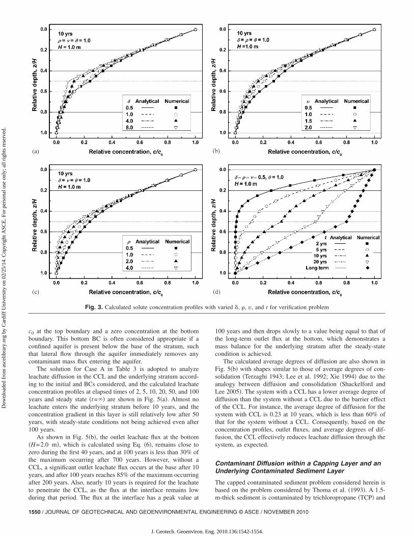
First, three series of analyses are performed, all with H=1.0 m and �=1, where the value of one of the parameters givenby Eq. �7� is varied while the other parameters are maintained atunity. Calculated solute concentration profiles at 10 years forthese three series of analyses are shown in Figs. 3�a–c�, respec-tively, together with those obtained by the numerical approach.The impact of the variation in the effective diffusion coefficientsand the porosities between the two layers can be clearly seen witha distinct change in the concentration gradient �i.e., shape of con-centration profile� at the interface from Figs. 3�a and c�. Thisresult is due to the fact that the interface BCs applied are depen-dent on the effective diffusion coefficients and the porosities �seeEq. �3b��. Such concentration gradient changes are not apparent inFig. 3�b� because the continuity in mass flux at the interface isindependent of retardation.

Solute concentration profiles at 2, 5, 10, and 20 years and forthe long term, for a case having �=�=�=0.5, �=1, and H=1.0 m, are presented in Fig. 3�d�, and the solute penetrationprocess can be seen clearly. The impact of the variation in effec-tive diffusion coefficients and the porosities between the two lay-ers can be seen at the interface in all but the 2-year profilebecause, at that short elapsed time, the solute has not yet reachedthe interface in any significant quanity.

Finally, a series of cases with �=�=�=0.5 and varying totalthicknesses �i.e., H=0.5,1.0,2.0 m� and different values of theratios of thickness for the lower layer relative to the upper layer�i.e., �=1 /3,1 ,3� are then considered, and the calculated resultsat 10 years are shown in Fig. 4. Comparison of the solute con-centration at the same relative depth in the lower layer shows theimpact of a thicker upper layer leading to significantly lower val-ues of solute concentration with increasing total thickness �i.e.,H�. This result is due to the increased time required to penetratethrough a thicker upper layer. Overall, the results of the verifica-tion analysis indicate that the analytical simulations are in excel-lent agreement with the numerical simulations.

Applications

In this section, the analytical solutions presented in this paper areapplied to analyze first leachate diffusion in a CCL and an under-lying stratum of a landfill and, second, contaminant diffusionwithin a capping layer and an underlying contaminated sedimentlayer.

Leachate Diffusion in a CCL and an UnderlyingStratum

CCLs typically have thicknesses of between 0.6 and 1.8 m �Ben-son and Daniel 1994� and a thickness of 0.9 m is consideredherein. The soil and transport properties for the CCL consideredare adopted from those presented by Lewis et al. �2009� and arelisted in Table 4 together with those for the underlying stratum. Aretardation factor of Rd=3.3 is adopted for the CCL following thevalues presented by Foose et al. �1999� for a similar material. Thethickness of the underlying stratum is assumed as 1.1 m. The
leachate concentration is assumed to be constant with a value of

2010.136:1542-1554.

Dm , Sm , Tm

m��dz+��h1

H c2,t=0�z�gm2�z�dz

− 1� + cz=H�0�h1

�m�� sin �m�cot��m�

�/�� + ��cos �m − � sin �m cot��m��2��1 + ��Am

2 �

1�z�dz + ��h1

H

��1 + � − z/h1�/�� + ��gm2�z�dz

/2��1 + ��Am2 �

�dz + ��h1

H

�� + �z/h1 − 1��/�� + ��gm2�z�dz

�h1/2��1 + ��Am2 �

xp��m��d�

xp��m��d�

m�

1�z�dz + ��h1

H


h1/2��1 + ��Am2 �

2

��Am2 �

m2 �

xp��m��d�

1546/JO

UR

NA

LO

FG

EO

TE

CH

NIC

AL

AN

DG

EO

EN

VIR

ON

ME

NT

AL

EN

GIN

EE

RIN

G©

AS

CE

/NO

VE

MB

ER

2010

Dow

nloa

ded

from

asc

elib

rary

.org

by

Car

diff

Uni

vers

ity o

n 02

/25/

14. C

opyr

ight

ASC

E. F

or p

erso

nal u

se o

nly;

all

righ

ts r

eser

ved.

Table 2. Analytical Solutions for Contaminant Diffusion in Double-Layered Soils, Scenarios with Various Combinations of BCs

ScenarioBoundaryconditions ci �m Am , Bm , Cm ,

1 c1 �z=0=cz=0�t�c2 �z=H=cz=H�t� c1 = f1�z,t� + �

m=1

�

�Bm + CmSm�t� + DmTm�t��gm1�z�exp�− �mt�

f1�z,t� = cz=0�t��1 − z/h1� + �

�� + �+ cz=H�t�

��z/h1

�� + �

gm1�z� = sin�mz

h1

c2 = f2�z,t� + �m=1

�

�Bm + CmSm�t� + DmTm�t��gm2�z�exp�− �mt�

f2�z,t� = cz=0�t�1 + � − z/h1

�� + �+ cz=H�t�

�� + �z/h1 − 1�� + �

gm2�z� = Am sin�mH − z

h1

�� sin �m cos��m�+cos �m sin��m�=0

Am=sin �m /sin��

Bm=�0h1c1,t=0�z�gm1�z

+ cz=0�0�h1

�m�cos �m

− csc��m��+ �− cz=0�0� + cz=H�0��h1/�m��

�h1/Cm =

−

�0

h1

��1 − z/h1� + ��/�� + ��gm

�h1

Dm =

−

�0

h1

��z/h1�/�� + ��gm1�z

Sm�t� =�0

tdcz=0��

d�e

Tm�t� =�0

tdcz=H��

d�e

2 c1 �z=0=cz=0�t�

� �c2

�z�

z=H

= 0ci = cz=0�t� + �

m=1

�

�Bm + CmSm�t��gmi�z�exp�− �mt�

gm1�z� = sin�mz

h1

gm2�z� = Am cos�mH − z

h1

�� sin �m sin��m�−cos �m cos��m�=0

Am=sin �m /cos��

Bm =

�0

h1

c1,t=0�z�gm

�

− cz=0�0��m�1 +

Cm = −2

�m�1 + ��A

Sm�t� =�0

tdcz=0��

d�e

J. Geotech. Geoenviron. Eng. 2010.136:1542-1554.

, Bm , Cm , Dm , Sm , Tm

��h1

H


+ ��Am2 �

− cz=H�0�2��Am

�m�1 + ��Am2 �

Dm = −2��Am

�m�1 + ��Am2 �

� =�0

tdcz=H��

d�exp��m��d�

�z�gm1�z�dz + ��h1

H


�h1/2��1 + ��Am2 �

c2,t=0�z�dz�h1/�m��sin �m + ��Am sin��m��

�h1/2��1 + ��Am2 �

JOU

RN

AL

OF

GE

OT

EC

HN

ICA

LA

ND

GE

OE

NV

IRO

NM

EN

TA

LE

NG

INE

ER

ING

©A

SC

E/N

OV

EM

BE

R2010

/1547

Dow

nloa

ded

from

asc

elib

rary

.org

by

Car

diff

Uni

vers

ity o

n 02

/25/

14. C

opyr

ight

ASC

E. F

or p

erso

nal u

se o

nly;

all

righ

ts r

eser

ved.

Table 2. �Continued.�

ScenarioBoundaryconditions ci �m Am

3 ��c1

�z�

z=0

= 0

c2 �z=H=cz=H�t�ci = cz=H�t� + �

m=1

�

�Bm + DmTm�t��gmi�z�exp�− �mt�

gm1�z� = cos�mz

h1

gm2�z� = Am sin�mH − z

h1

sin �m sin��m�−�� cos �m cos��m�=0

Am=cos �m /sin��m�

Bm =

�0

h1

c1,t=0�z�gm1�z�dz +

�h1/2��1

Tm�t

4 � �c1

�z�

z=0

= 0

� �c2

�z�

z=H

= 0 ci =

�0

h1

ct=0�z�dz + ��h1

H

ct=0�z�dz

h1 + ��h2+ �

m=1

�

Bmgmi�z�

exp�− �mt�

gm1�z� = cos�mz

h1

gm2�z� = Am cos�mH − z

h1

sin �m cos��m�+�� cos �m sin��m�=0

Am=cos �m /cos��m�

Bm =

�0

h1

c1,t=0

−

�0

h1

c1,t=0�z�dz + ��h1

H

h1 + ��h2

Note:=�� /�; �m= �D1� /Rd1� ��m

2 /h12�.


Uc

�m=1

�

��1 − cos �m� + ��Am/��1 − cos��m��Bm/�m�exp�− �mt�

�c0/�� + �� + ��/2� + ��2�/2��

�m=1

�


�1 + ��c0

�m=1

�


��c0

�m=1

�

��1 − cos �m� + ��Am/�sin��m��Bm/�m�exp�− �mt�

�1 + ��c0

�m=1

�


�1 + ��c0

1548/JO

UR

NA

LO

FG

EO

TE

CH

NIC

AL

AN

DG

EO

EN

VIR

ON

ME

NT

AL

EN

GIN

EE

RIN

G©

AS

CE

/NO

VE

MB

ER

2010

Dow

nloa

ded

from

asc

elib

rary

.org

by

Car

diff

Uni

vers

ity o

n 02

/25/

14. C

opyr

ight

ASC

E. F

or p

erso

nal u

se o

nly;

all

righ

ts r

eser

ved.

Table 3. Analytical Solutions for Contaminant Diffusion in Double-Layered Soils with Particular Initial and BCs

Case Initial Boundary ci�z , t� �m , Am Bm

A c1 �t=0=0c2 �t=0=0

c1 �z=0=c0c2 �z=H=0 c1 = c0

��1 − z/h1� + �

�� + �

+ �m=1

�

Bm sin�mz

h1exp�− �mt�

c2 = c01 + � − z/h1

�� + �

+ �m=1

�

AmBm sin�mH − z


�� sin �m cos��m�+cos �m sin��m�=0Am=sin �m /sin��m�

c0��m cos �m − ��m − ��m + ��m sin �m cot��m�

�m2 �� + ��1 + ��Am

2 �/2

1 +

B c1 �t=0=c0c2 �t=0=c0

c1 �z=0=0c2 �z=H=0

c1 = �m=1

�

Bm sin�mz


c2 = �m=1

�

AmBm sin�mH − z


As abovec0

1 + ��Am

�m�1 + ��Am2 �/2

1 −

C c1 �t=0=0c2 �t=0=c0

As above As above As abovec0

��Am�1 − cos��m��m�1 + ��Am

2 �/2

1 −

D c1 �t=0=0c2 �t=0=0

c1 �z=0=c0�dc2 / dz �z=H=0

c1 = c0 + �m=1

�

Bm sin�mz


c2 = c0 + �m=1

�

AmBm cos�mH − z


�� sin �m sin��m�−cos �m cos��m�=0Am=sin �m /cos��m�

−2c0

�m�1 + ��Am2 �

1 +

E c1 �t=0=c0c2 �t=0=c0

c1 �z=0=0�dc2 / dz �z=H=0

c1 = �m=1

�

Bm sin�mz


c2 = �m=1

�

AmBm cos�mH − z


As above 2c0

�m�1 + ��Am2 �

1 −


Uc

�m=1

�


��c0

/

JOU

RN

AL

OF

GE

OT

EC

HN

ICA

LA

ND

GE

OE

NV

IRO

NM

EN

TA

LE

NG

INE

ER

ING

©A

SC

E/N

OV

EM

BE

R2010

/1549

Dow

nloa

ded

from

asc

elib

rary

.org

by

Car

diff

Uni

vers

ity o

n 02

/25/

14. C

opyr

ight

ASC

E. F

or p

erso

nal u

se o

nly;

all

righ

ts r

eser

ved.

Table 3. �Continued.�

Case Initial Boundary ci�z , t� �m , Am Bm

F c1 �t=0=0

c2 �t=0=c0

As above As above As abovec0

��Am sin��m��m�1 + ��Am

2 �/2

1 −

G c1 �t=0=0

c2 �t=0=c0�dc1

dz�

z=0

= 0

�dc2

dz�

z=H

= 0

c1 = c0��

1 + ��+ �

m=1

�

Bm cos�mz

h1exp�

− �mt�

c2 = c0��

1 + ��+ �

m=1

�

AmBm cos�mH − z

h1

exp�− �mt�

sin �m cos��m�+�� cos �m sin��m�=0

Am

=cos �m /cos��m�

c0− �� sin �m + ��Am sin��m�

�m�1 + ��1 + ��Am2 �/2

Note:=�� /�; �m= �D1� /Rd1� ��m

2 /h12�.


Dow

nloa

ded

from

asc

elib

rary

.org

by

Car

diff

Uni

vers

ity o

n 02

/25/

14. C

opyr

ight

ASC

E. F

or p

erso

nal u

se o

nly;

all

righ

ts r

eser

ved.

c0 at the top boundary and a zero concentration at the bottomboundary. This bottom BC is often considered appropriate if aconfined aquifer is present below the base of the stratum, suchthat lateral flow through the aquifer immediately removes anycontaminant mass flux entering the aquifer.

The solution for Case A in Table 3 is adopted to analyzeleachate diffusion in the CCL and the underlying stratum accord-ing to the initial and BCs considered, and the calculated leachateconcentration profiles at elapsed times of 2, 5, 10, 20, 50, and 100years and steady state �t=�� are shown in Fig. 5�a�. Almost noleachate enters the underlying stratum before 10 years, and theconcentration gradient in this layer is still relatively low after 50years, with steady-state conditions not being achieved even after100 years.

As shown in Fig. 5�b�, the outlet leachate flux at the bottom�H=2.0 m�, which is calculated using Eq. �6�, remains close tozero during the first 40 years, and at 100 years is less than 30% ofthe maximum occurring after 700 years. However, without aCCL, a significant outlet leachate flux occurs at the base after 10years, and after 100 years reaches 85% of the maximum occurringafter 200 years. Also, nearly 10 years is required for the leachateto penetrate the CCL, as the flux at the interface remains low

Fig. 3. Calculated solute concentration profile

during that period. The flux at the interface has a peak value at



100 years and then drops slowly to a value being equal to that ofthe long-term outlet flux at the bottom, which demonstrates amass balance for the underlying stratum after the steady-statecondition is achieved.

The calculated average degrees of diffusion are also shown inFig. 5�b� with shapes similar to those of average degrees of con-solidation �Terzaghi 1943; Lee et al. 1992; Xie 1994� due to theanalogy between diffusion and consolidation �Shackelford andLee 2005�. The system with a CCL has a lower average degree ofdiffusion than the system without a CCL due to the barrier effectof the CCL. For instance, the average degree of diffusion for thesystem with CCL is 0.23 at 10 years, which is less than 60% ofthat for the system without a CCL. Consequently, based on theconcentration profiles, outlet fluxes, and average degrees of dif-fusion, the CCL effectively reduces leachate diffusion through thesystem, as expected.

Contaminant Diffusion within a Capping Layer and anUnderlying Contaminated Sediment Layer

The capped contaminated sediment problem considered herein isbased on the problem considered by Thoma et al. �1993�. A 1.5-

varied �, �, v, and t for verification problem
s with
m-thick sediment is contaminated by trichloropropane �TCP� and


2010.136:1542-1554.

Dow

nloa

ded

from

asc

elib

rary

.org

by

Car

diff

Uni

vers

ity o

n 02

/25/

14. C

opyr

ight

ASC

E. F

or p

erso

nal u

se o

nly;

all

righ

ts r

eser

ved.

covered by a 0.7-m-thick balsam sand capping layer to impedethe TCP from dispersing into the surface water. The soil andtransport properties considered for these two layers are as definedby Thoma et al. �1993� and are summarized in Table 5. The initialconcentration of TCP is 150 mg/L for the sediment �cs �t=0

Fig. 4. Calculated solute concentration profiles with varied � and Hfor verification problem

=150 mg /L� and zero for the capping layer. A zero-flux BC is



imposed at the bottom of the sediment layer, and the concentra-tion is fixed at zero at the top of the capping layer to model thewashing effect of the surface water. This scenario matches Case Fpreviously defined in Table 3.

The resulting TCP concentration distributions in both the cap-ping layer and the sediment layer at different elapsed times areshown in Fig. 6�a�. In order to evaluate the impact of the cappinglayer on containment, a scenario without the capping layer is alsoconsidered and can be analyzed by the solution for Case E inTable 3 or the analytical solution presented by Carslaw and Jaeger�1959� and Shackelford and Lee �2005�. In this analysis the sedi-ment layer is arbitrarily separated into 0.5- and 1.0-m-thick lay-ers, and the soil and transport properties of the sediment are setfor both of the two layers. The concentration profiles for the sce-nario without the capping layer are shown in Fig. 6�b�. Based on

Table 4. Soil and Transport Properties for CCL and Underlying Stratum

Property �unit� CCLa Underlying stratum

D� �m2 /s� 4�10−10 1�10−10

Rd 3.3 1.0

n 0.444 0.375

h �m� 0.9 1.1aFrom Lewis et al. �2009� and Foose et al. �1999�.

Fig. 5. Calculated leachate concentration profiles, average degree ofdiffusion, and leachate flux for diffusion in the CCL and the under-lying stratum of a landfill

Table 5. Soil and Transport Properties for Capping Layer and Contami-nated Sediment �Thoma et al. 1993�

Property �unit� Capping material Sediment

D� �m2 /s� 9.8�10−10 9.4�10−10

Rd 4.94 43.3

n 0.38 0.45

h �m� 0.7 1.5


2010.136:1542-1554.

Dow

nloa

ded

from

asc

elib

rary

.org

by

Car

diff

Uni

vers

ity o

n 02

/25/

14. C

opyr

ight

ASC

E. F

or p

erso

nal u

se o

nly;

all

righ

ts r

eser

ved.

comparison of the concentration profiles after 10 years, less TCPhas been removed from the sediment for the scenario with thecapping layer, as expected.

Fig. 6. Calculated TCP concentration profiles at different times fordiffusion in �a� capped contaminated sediment; �b� uncapped con-taminated sediment

capped contaminated sediment problem considered here. An in-



This observation can be observed more clearly in Fig. 7, wherethe average degree of diffusion, Uc, for both the scenarios �withand without the cap� versus time is presented. For the scenariowith a capping layer Uc is close to zero corresponding to almostno TCP diffusion into water for the first 10 years and only 3.7%of TCP has diffused into water after 100 years. However, valuesfor Uc of 6.2 and 20% within the first 10 and 100 years, respec-tively, result for the scenario without the capping layer.

For the scenarios considered above, the rate of TCP diffusioninto the water is quite low, and more than 1,000 years are requiredto reach an average degree of diffusion of 90%. This result is to alarge extent caused by the high retardation factor of the sediment.To assess the impact of the retardation factor on the system, anadditional analysis was performed with the retardation factor ofthe sediment given a significantly lower value �matching that ofthe capping layer�. The resulting calculated average degrees ofdiffusion with time are also illustrated in Fig. 7. The rate of TCPdiffusion is considerably greater, with average degrees of diffu-sion of 22 and 58% after 100 years for the scenarios with andwithout the cap, respectively. This result clearly shows that theretardation factor of porous media is of importance for the rate ofcontamination diffusion. The analyses presented herein do notinclude the effect of consolidation of both the sediment and un-derlying uncontaminated layers on the TCP transport which couldresult in greater TCP mass flux due to advection �Alshawabkehet al. 2005; Arega and Hayter 2008�. However, the analyticalsolutions presented in this paper can be regarded as a useful ap-proach to predict the lower boundary of the rate of contaminanttransport from the sediment.

The definition of average degree of diffusion used in thispaper, i.e., Eq. �4�, represents the relative amount of solute massremoved or gained in the double layers following the approach ofShackelford and Lee �2005�. However, another definition basedon solute mass in pore water presented by Chen et al. �2009� canbe written for a double-layer porous medium as follows:

Uc�t� =

�0

h1

c1�z,0�dz +�h1

H

c2�z,0�dz −�0

h1

c1�z,t�dz −�h1

H

c2�z,t�dz

�0

h1

c1�z,0�dz +�h1

H

c2�z,0�dz −�0

h1

c1�z,��dz −�h1

H

c2�z,��dz

�21�

Considering Case F, the average degree of diffusion based on Eq.�21� and solute mass in pore water can then be written as follows:

Uc�t� = 1

−

�m=1

�

��1 − cos �m� + �Am/�sin�e�m��Bm/�m�exp�− �mt�

ec0

�22�

The calculated average degrees of diffusion for both definitions�i.e., Eqs. �4� and �22�� are plotted versus time in Fig. 8 for the

teresting outcome is that, when based on solute mass in the porewater, the value of average degree of diffusion is negative in thefirst 300 years of the analysis. This is a result of the relativelyhigh retardation factor of the sediment compared to that of thecapping layer. The solute mass diffusing from the sediment intothe cap leads to a small reduction of solute concentration in thesediment, but a relatively large increase in solute concentration inthe capping layer. This results in a greater average solute concen-tration through the double layers than that at the initial state, andsubsequently according to the definition of average degree of dif-fusion given in Eq. �22� a negative average degree of diffusionduring the early period, which is clearly problematic. However, as
shown in Fig. 8, the average degree of diffusion based on solute

2010.136:1542-1554.

Dow

nloa

ded

from

asc

elib

rary

.org

by

Car

diff

Uni

vers

ity o

n 02

/25/

14. C

opyr

ight

ASC

E. F

or p

erso

nal u

se o

nly;

all

righ

ts r

eser

ved.

mass in the soil, as defined by Shackelford and Lee �2005� andapplied in this paper for a two-layered system �i.e., Eq. �4��,avoids this problem as the total mass of contaminant which isconserved is considered. Consequently, the average degree of dif-fusion based on total contaminant mass is more reasonable thanthat based on solute mass in the pore water �solute concentration�.

Consideration of Eq. �6� allows the following expression to bedeveloped to calculate the TCP flux into the water:

Jc�t� = −n1D1

�

h1�m=1

�

�mBm exp�− �mt� �23�

The calculated TCP fluxes into the water for both the scenarioswith and without the capping layer, considering the original retar-dation factor, are shown in Fig. 9�a�. The maximum flux for thescenario without the capping layer is more than 200 times greaterthan that for the scenario with the capping layer, and this maxi-mum flux occurs at the start of the analysis and subsequentlydecreases with the time. However, the flux for the scenario withthe capping layer is close to zero within the first 3 years as thecapping layer prevents TCP from diffusing directly into the water.The TCP concentration then increases due to the penetrationthrough the capping layer, reaching a maximum �i.e., 6.06�10−8 g /s m2� at the elapsed time of 45 years and decreasesthereafter. Following the definition of breakthrough by Palermoet al. �1998a�, the flux reaches 5% of its maximum value at theelapsed time of 4.25 years. These results, when considered withthe average degree of diffusion shown in Fig. 7, clearly demon-strate the impact of introducing a capping layer to the system bothin terms of timescales and levels of contaminant flux.

Fig. 7. Calculated average degree of diffusion with time for diffusionin a capped contaminated sediment

Fig. 8. Comparison of different definitions of average degree of dif-fusion for diffusion in a capped contaminated sediment



An analytical solution for diffusion in a finite homogeneousmedium presented by Carslaw and Jaeger �1959� is often em-ployed to estimate the solute diffusion in the capping layer forcapping contaminated sediment �Thoma et al. 1993; Palermoet al. 1998a,b�, with an assumption of constant concentration atthe bottom of the capping layer. A similar analytical solution for asemiinfinite medium with the same BC has also been presentedby Carslaw and Jaeger �1959�. The solute flux from the top sur-face of the capping, based on these two analytical solutions forfinite and semiinfinite media �Carslaw and Jaeger 1959�, can beexpressed as follows:

Jc�t� =n1D1

�c0

h1�1 + 2�

m=1

�

�− 1�m

exp−m22D1

�t

Rd1h12 � �finite media� �24�

Jc�t� = n1D1�c0� Rd1

D1�t

exp−Rd1h1

2

4D1�t �semiinfinite media�

�25�

These two alternative solutions can be used to compare the resultsof the solutions developed in this paper that consider the contami-nated sediment layer with those that do not consider the contami-nated sediment layer.

The calculated TCP fluxes into water using Eqs. �24� and �25�are illustrated in Fig. 9�b�. The fluxes remain low in the first 3years, which is in good agreement with the result calculated usingthe analytical solution presented in this paper. However, the TCPflux calculated by the analytical solution for a finite medium �i.e.,Eq. �24�� then increases rapidly and reaches a peak value at 65

−8 2

Fig. 9. Calculated TCP flux into water with time for diffusion in acapped contaminated sediment ��a� analytical solution for a finitemedium; �b� analytical solution for a semiinfinite medium�

years of 7.98�10 g /s m , which is 31.7% more than that ob-


2010.136:1542-1554.

Dow

nloa

ded

from

asc

elib

rary

.org

by

Car

diff

Uni

vers

ity o

n 02

/25/

14. C

opyr

ight

ASC

E. F

or p

erso

nal u

se o

nly;

all

righ

ts r

eser

ved.

tained by the analytical solution presented in this paper. The fluxthen remains at this peak value thereafter as a steady state, linearsolute concentration distribution within the capping has beenreached. The TCP flux calculated by the analytical solution for aninfinite medium �i.e., Eq. �25�� has a peak value of 3.86�10−8 g /s m2 at 37.5 years, which is 36.3% less than that ob-tained by the analytical solution presented in this paper and de-creases slowly thereafter. However, the analytical solution for aninfinite medium overestimates the TCP flux in the long term �after6,750 years�, as shown in Fig. 9�b�. Consequently, the solute fluxfrom the capping layer into water may be overestimated by theanalytical solution for a finite medium and underestimated by thatfor a semiinfinite medium, i.e., during timescales typically con-sidered in engineering applications.

Conclusions

Analytical solutions for conservative solute diffusion in one-dimensional double-layered porous media were presented in thispaper. Solutions were derived for various combinations of fixedsolute concentration and zero-flux BCs at the top and the bottomand for arbitrary initial solute concentration distributions through-out the media. Several solutions considering particular initial andBCs were presented based on typical contaminant transport prob-lems found in geoenvironmental engineering. These analytical so-lutions were shown to correlate well with numerical solutionsfrom a finite-element analysis.

The presented analytical solutions were used to investigateleachate transport for two typical applications: �1� a CCL from alandfill with an underlying stratum and �2� contaminant diffusionwithin a subaqueous capped contaminated sediment system. Analternative definition of the average degree of diffusion based onsolute concentration was also considered and found to be lessrobust than the definition based on total solute mass adopted inthis paper. Furthermore, for the capped contaminated sedimentapplication, comparisons with alternative solutions indicated thatconsideration of the contaminated sediment layer is necessary toobtain reasonable estimates of contaminant fluxes from the cap-ping layer.

Acknowledgments

The financial support received from the U.K. Engineering andPhysical Sciences Research Council via Grant No. EP/C532651/2and from the National Natural Science Foundation of China�NSFC�, Grant Nos. 10972195 and 51009121 are gratefullyacknowledged.

References

Alshawabkeh, A. N., Rahbar, N., and Sheahan, T. �2005�. “A model forcontaminant mass flux in capped sediment under consolidation.” J.Contam. Hydrol., 78�3�, 147–165.

Arega, F., and Hayter, E. �2008�. “Coupled consolidation and contami-nant transport model for simulating migration of contaminantsthrough the sediment and a cap.” Appl. Math. Model., 32�11�, 2413–2428.

Benson, C. H., and Daniel, D. E. �1994�. “Minimum thickness of com-pacted soil liners. 2. Analysis and case-histories.” J. Geotech. Engrg.,120�1�, 153–172.

Carslaw, H. S., and Jaeger, J. C. �1959�. Conduction of heat in solids,Oxford University Press, New York.

Chapra, S. C., and Canale, R. P. �2006�. Numerical methods for engi-neers, McGraw-Hill Higher Education, Boston.



Chen, Y., Xie, H., Ke, H., and Chen, R. �2009�. “An analytical solutionfor one-dimensional contaminant diffusion through multi-layered sys-tem and its applications.” Environ. Geol., 58�5�, 1083–1094.

Cleall, P. J., Seetharam, S. C., and Thomas, H. R. �2007�. “Inclusion ofsome aspects of chemical behavior of unsaturated soil in thermo/hydro/chemical/mechanical models. I: Model development.” J. Eng.Mech., 133�3�, 338–347.

Crank, J. �1956�. The mathematics of diffusion, Oxford University Press,New York.

Foose, G. J., Benson, C. H., and Edil, T. B. �1999�. “Equivalency ofcomposite geosynthetic clay liners as a barrier to volatile organiccompounds.” Geosynthetics 99, Industrial Fabrics Association Inter-national, Roseville, Minn., 321–334.

Freeze, R. A., and Cherry, J. A. �1979�. Groundwater, Prentice-Hall,Englewood Cliffs, N.J.

Lampert, D. J., and Reible, D. �2009�. “An analytical modeling approachfor evaluation of capping of contaminated sediments.” Soil SedimentContam., 18�4�, 470–488.

Lee, P. K. K., Xie, K. H., and Cheung, Y. K. �1992�. “A study on one-dimensional consolidation of layered systems.” Int. J. Numer. Analyt.Meth. Geomech., 16�11�, 815–831.

Leij, F. J., Dane, J. H., and van Genuchten, M. T. �1991�. “Mathematical-analysis of one-dimensional solute transport in a layered soil-profile.”Soil Sci. Soc. Am. J., 55�4�, 944–953.

Leij, F. J., and van Genuchten, M. T. �1995�. “Approximate analyticalsolutions for solute transport in two-layer porous-media.” Transp. Po-rous Media, 18�1�, 65–85.

Lewis, T. W., Pivonka, P., Fityus, S. G., and Smith, D. W. �2009�. “Para-metric sensitivity analysis of coupled mechanical consolidation andcontaminant transport through clay barriers.” Comput. Geotech.,36�1–2�, 31–40.

Liu, C., and Ball, W. P. �1998�. “Analytical modeling of diffusion-limitedcontamination and decontamination in a two-layer porous medium.”Adv. Water Resour., 21�4�, 297–313.

Liu, C., Ball, W. P., and Ellis, J. H. �1998�. “An analytical solution to theone-dimensional solute advection-dispersion equation in multi-layerporous media.” Transp. Porous Media, 30�1�, 25–43.

Palermo, M. R., et al. �1998a�. Guidance for subaqueous dredged mate-rial capping, U.S. Army Corps of Engineers, Vicksburg, Miss.

Palermo, M. R., Maynord, S., Miller, J., and Reible, D. D. �1998b�.Guidance for in-situ subaqueous capping of contaminated sediments,Great Lakes National Program Office, Chicago.

Rowe, R. K., Quigley, R. M., Brachman, R. W. I., and Booker, J. R.�2004�. Barrier systems for waste disposal facilities, Taylor & Fran-cis, Oxford, U.K.

Seetharam, S. C., Thomas, H. R., and Cleall, P. J. �2007�. “Coupledthermo/hydro/chemical/mechanical model for unsaturated soils—Numerical algorithm.” Int. J. Numer. Methods Eng., 70, 1480–1511.

Shackelford, C. D. �1991�. “Laboratory diffusion testing for waste dis-posal: A review.” J. Contam. Hydrol., 7�3�, 177–217.

Shackelford, C. D., and Daniel, D. E. �1991�. “Diffusion in saturated soil.I: Background.” J. Geotech. Geoenviron. Eng., 117�3�, 467–484.

Shackelford, C. D., and Lee, J. M. �2005�. “Analyzing diffusion by anal-ogy with consolidation.” J. Geotech. Geoenviron. Eng., 131�11�,1345–1359.

Sharma, H. D., and Reddy, K. R. �2004�. Geoenvironmental engineering:Site remediation, waste containment, and emerging waste manage-ment technologies, Wiley, New York.

Taylor, D. W. �1948�. Fundamentals of soil mechanics, Wiley, New York.Terzaghi, K. �1943�. Theoretical soil mechanics, Wiley, New York.Thoma, G. J., Reible, D. D., Valsaraj, K. T., and Thibodeaux, L. J. �1993�.

“Efficiency of capping contaminated sediments in-situ. 2. Mathemat-ics of diffusion adsorption in the capping layer.” Environ. Sci. Tech-nol., 27�12�, 2412–2419.

Xie, K. H. �1994�. “Theory of one dimensional consolidation of double-layered ground and its applications.” Chinese J. Geotech. Eng., 16�5�,26–38.


2010.136:1542-1554.

analytical solutions for contaminant diffusion in …orca.cf.ac.uk/8277/1/li.pdf · analytical...

Documents