an analytical solution for contaminant transport against … · most existing analytical solutions...
TRANSCRIPT
INTERNATIONAL JOURNAL OF ENVIRONMENTAL SCIENCES Volume 3, No 2, 2012
© Copyright by the authors - Licensee IPA- Under Creative Commons license 3.0
Research article ISSN 0976 – 4402
Received on November 2012 Published on December 2012 1208
An analytical solution for contaminant transport against the flow with
periodic boundary condition in one-dimensional porous media Yadav R.R, Dilip Kumar Jaiswal,
Gulrana
Department of Mathematics and Astronomy, Lucknow University
Lucknow-226007, India
doi:10.6088/ijes.2012030133029
ABSTRACT
The transport of pollutants in porous media, is of hydrodynamic dispersion phenomena, has
been the major research subject for more than four decades. The present paper is an attempt
to describe analytically the solute transport in one-dimensional homogeneous porous medium
of finite domain. The effects of time-periodic pulse-type inlet contaminant concentration and
groundwater flow velocity against the contaminant transport are investigated analytically.
The temporally dependent dispersion proportional to seepage velocity and retardation factor
is also taken into account. The governing transport equation is solved analytically by
employing Laplace transformation technique. The effects of various physical parameters on
solute transport and their importance are discussed and are also illustrated graphically.
Keywords: Dispersion, pollutant, retardation factor, seepage flow.
1. Introduction
From several decades, the factory activities and uncontrolled use of pesticides in agriculture
cause serious damages on the environment in the area and affected groundwater table. The
characteristics of pollutants level and transport in groundwater are associated with variations
in one or two parameters at one scale and several parameters at another scale. Pollutant
behavior in the soil system is subject to many processes. The water soil system is dynamic
and many chemical, biological and physical reaction occurs which may affect pollutant
behavior. Solute transport inside the aquifer systems is due to hydrodynamic dispersion.
Mathematical model is one of the powerful tools to predict the effect of pollution on the long
term water resource quality. Most existing analytical solutions for advection–diffusion
transport problems including sorption, retardation and decay terms are for semi-infinite or
infinite regions. The dispersion coefficient during solute transport in the aquifer was studied
by Ogata and Banks (1961), Hoopes and Harleman (1967), Gelhar and Collins (1971). They
assumed that the aquifer consists of a geologically homogeneous porous medium. Kumar
(1983) presented time-dependent input concentration against exponentially decreasing
unsteady velocity. Frind (1982) presented a finite element solution using a velocity-
dependent dispersion coefficient and discussed the errors caused by use of a constant
dispersion coefficient. Volker and Rushton (1982) compared a variety of aquifer parameters
and the influence of the flow conditions on the configuration and location of the interface.
Many studies assume a steady state flow field. However, natural flow systems are rarely in a
steady state. Temporal fluctuations in the recharge or in the boundary conditions lead to
variations in the velocity field that contribute to dispersive mixing. Field studies of the
groundwater discharge process in unconfined coastal aquifers show that the tide can

An analytical solution for contaminant transport against the flow with periodic boundary condition in one-
dimensional porous media
Yadav R.R, Dilip Kumar Jaiswal, Gulrana
International Journal of Environmental Sciences Volume 3 No.3, 2012 1209
significantly influence the temporal and spatial patterns of groundwater discharge as well as
the salt concentration in the near-shore groundwater (Robinson et al. 1998; Groundwater
fluctuations as induced by oceans oscillations affect water and mass exchange between
aquifer and ocean (Li et al. 1999,1999a). The period of the fluctuations of the downstream
water level affects the oscillations of the hydraulic heads and therefore the velocities within
the aquifer. The effect of flow oscillations on solute transport in tubes has been investigated
by several researchers. Since contaminants in porous medium migrate with ground water
flow, any factors that may affect groundwater flow are also likely to influence the migration
of contaminants in porous media. Time periodic convection leading to the dispersion of
Brownian particle in solution may be observed in the transport of contaminant in tidal
estuaries (Bowden; 1965), the spread tracer in blood vessels (Caro; 1966), the mixing of salt
water with fresh water in coastal aquifer (Bear; 1972). Watson (1983) determined that solute
dispersion effects along a pipe due to steady and oscillatory flow are additive. Oscillatory
flow has also been found to influence dispersion in tubes. Fang et al. (1972) simulate the tidal
fluctuation of the groundwater table, by using a two-dimensional finite element model.
Custodio (1988) discussed that in many real situations, such as sluggish freshwater flow,
stresses caused by tidal oscillations and recharge events, and enhanced dispersivity by
macroscopic heterogeneities. Townley (1993, 1995) presented a periodic finite element
model called AQUIFEM-P that computes periodic fluctuations in heads and velocities in a 2-
D region of aquifer. Logan and Zlotnik (1995) obtained solutions of the convection–diffusion
equation with decay for periodic boundary conditions on a semi–infinite domain. The
boundary conditions take the form of a periodic concentration or a periodic flux, and a
transformation is obtained that relates the solutions of the two, pure boundary value problems.
Krabbenhoft and Webster (1995) study the influence of periodic flow reversals on temporal
variation in the water chemistry of a shallow seepage lake in Michigan. Ataie-Ashtiani (1998)
validated the model for simulation of groundwater flow in response to the periodic boundary
condition in unconfined aquifers with a mild sloping face. Andricˇevic´ and Cvetkovic´
(1998) reported the solute flux as a function of travel time and transverse displacement in the
relative dispersion frame work by removing the plume meandering.
Many analytical solutions have been derived to describe the periodic groundwater flow (Li et
al.; 2001, Jeng et al.; 2002). Common problems include salt-water intrusion due to over
pumping of groundwater and brine discharges from desalination plants, as well as coastal
water pollution by plume leachate from contaminated coastal aquifers (Purnalna et al.; 2003,
Masciopinto; 2006,). Song et al. (2007) presented a new perturbation solution of the non-
linear Boussinesq equation for one-dimensional tidal groundwater flow in a coastal aquifer.
Jaiswal et al. (2009) and Kumar et al. (2010) obtained analytical solutions for temporally and
spatially dependent solute dispersion in a one dimensional semi-infinite porous medium.
Yadav et al. (2010) obtained analytical solutions of one-dimensional advection–dispersion
equation in semi-infinite longitudinal porous domain.
In most hydrological situations contaminant and groundwater flow may vary with time.
Contaminant input may varying frequently, weekly, monthly or even on annual basis.
Similarly, groundwater flow might be considered likely vary periodically as a result of
downfall patterns. The objective of this paper is to address the influence of periodic seepage
velocity on the porous medium and consequently on the transport of solute under periodic
condition. Also, developed an analytical solution which is represent contaminant
concentrations in groundwater systems under periodic seepage flow velocity. In present study,
non-reactive pollutants are considered in finite Porous domain. The direction of periodic
seepage flow is from to . A source concentration (periodic pulse type) is

An analytical solution for contaminant transport against the flow with periodic boundary condition in one-
dimensional porous media
Yadav R.R, Dilip Kumar Jaiswal, Gulrana
International Journal of Environmental Sciences Volume 3 No.3, 2012 1210
enforced at the boundary , i.e., against the flow while mixed type boundary condition
is assumed at . Initially the domain is not solute free. Retardation factor is also
considered. Laplace Transformation technique (LTT) is used to get the analytical result of the
proposed problem.
2. Mathematical formulation and analytical solution
The transport of solutes in saturated, homogeneous porous media, accounting for one-
dimensional hydrodynamic dispersion is governed by the following partial differential
equation,
(1) where is a retardation factor accounting for equilibrium linear
sorption processes and describing solute sorption, is porosity, is empirical constant.
The use of equilibrium isotherms assumes that equilibrium exists at all times between the
porous medium and the solute in solution. This assumption is generally valid when the
adsorption process is fast in relation to the ground-water velocity. is the solute
concentration in the liquid phase at position and time . The dispersion coefficient,
presumably includes the effects of both molecular diffusion and mixing in the axial direction,
however molecular diffusion is negligible due to very low seepage velocity. In Eq. (1), and
may be constants or function of time. If both the parameters are independent to independent
variables and , then these are called constant dispersion and uniform flow velocity
respectively. The term on the left side of the equal sign indicate the retardation factor and
change of concentration in time, the first two terms on the right side describe hydrodynamic
dispersion and groundwater velocity.
Let the porous domain is of finite length. Initially the domain is not solute free, it is
exponentially increasing function of space variable. A pulse type input contaminants are
being introduced till time , where the time of illumination of source concentration,
beyond that source becomes zero. Contaminants will move against the direction of flow and
spread out with time due to higher concentration. On other hand, mixed type boundary
condition is assumed at . This type of situation generally exist saline water intrusion
into coastal aquifer. Under these assumptions mathematically, initial and boundary conditions
of proposed problem can be written as,
, ,
(2)
,
(3a)
, ,
(3b)
where is the resident concentration and is a constant which is less than one and its
dimension is inverse of space variable . Eq. (2) shows that the initial condition is an
increasing exponentially function of and unsteady coefficient of dimension of inverse of
time . An input concentration of periodic nature is assumed at the one point of the domain
i.e., . The field observations indicate the source concentration may not be negative,
therefore is taken. The coefficient of dispersion is considered directly
proportional to seepage velocity (Yim and Mohsen, 1992), i.e.,
.

An analytical solution for contaminant transport against the flow with periodic boundary condition in one-
dimensional porous media
Yadav R.R, Dilip Kumar Jaiswal, Gulrana
International Journal of Environmental Sciences Volume 3 No.3, 2012 1211
Let us write , so that , where and are as
dimension of is hence it is initial diffusion coefficient. But initial diffusion
coefficient is zero at . But at i.e., represents the peak value
of . Similarly
may be interpreted, and the dimension of is , respectively.
is a unsteady parameter whose dimension is inverse to that the time variable . At ,
and are equal to zero, so Eq. (1) is valid in domain. Eq. (1) may be written in
absolute form as,
(4)
Let us introduce a new time variable using the following transformation (Crank, 1975),
or as the in domain.
or
(5)
Now differential equation (4) reduces into constant coefficients as
(6)
The conditions in terms of new time variable may be written as
, ,
(7)
,
(8a)
, ,
(8b)
Now introducing a new dependent variable by following transformation
(9)
The set of Eqs. (6), (7) and (8a,b) reduced into
(10)
, ,
(11)
,
(12a)
where ,
, ,
(12b)

An analytical solution for contaminant transport against the flow with periodic boundary condition in one-
dimensional porous media
Yadav R.R, Dilip Kumar Jaiswal, Gulrana
International Journal of Environmental Sciences Volume 3 No.3, 2012 1212
Applying Laplace transformation on equations (10) – (12), we have
(13)
, (14a)
(14b) ,
Thus the general solution of equation (13) may be written as
;
(15)
Using conditions (14a,b) on the above solution, we get
(16)
and
(17)
Thus the solution in the Laplacian domain may be written as

An analytical solution for contaminant transport against the flow with periodic boundary condition in one-
dimensional porous media
Yadav R.R, Dilip Kumar Jaiswal, Gulrana
International Journal of Environmental Sciences Volume 3 No.3, 2012 1213
or
(18)
Taking inverse Laplace transform of equation (18) which are discussed in Appendix, the
solution of advection-dispersion solute transport for periodic input condition in terms of
as,
;
(19a)
; (19b)
where
,
,
An analytical solution for contaminant transport against the flow with periodic boundary condition in one-
dimensional porous media
Yadav R.R, Dilip Kumar Jaiswal, Gulrana
International Journal of Environmental Sciences Volume 3 No.3, 2012 1214
,
, , and .
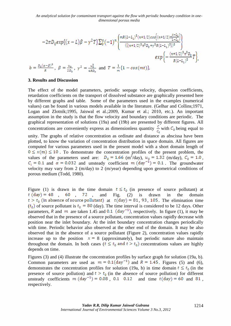
3. Results and Discussion
The effect of the model parameters, periodic seepage velocity, dispersion coefficients,
retardation coefficients on the transport of dissolved substance are graphically presented here
by different graphs and table. Some of the parameters used in the examples (numerical
values) can be found in various models available in the literature. (Gelhar and Collins;1971,
Logan and Zlotnik;1995, Jaiswal et al.;2009, Kumar et al.; 2010, etc.). An important
assumption in the study is that the flow velocity and boundary conditions are periodic. The
graphical representation of solutions (19a) and (19b) are presented by different figures. All
concentrations are conveniently express as dimensionless quantity with being equal to
unity. The graphs of relative concentration as ordinate and distance as abscissa have been
plotted, to know the variation of concentration distribution in space domain. All figures are
computed for various parameters used in the present model with a short domain length of
. To demonstrate the concentration profiles of the present problem, the
values of the parameters used are: (m2/day), (m/day), ,
and and unsteady coefficient . The groundwater
velocity may vary from 2 (m/day) to 2 (m/year) depending upon geometrical conditions of
porous medium (Todd, 1980).
Figure (1) is drawn in the time domain (in presence of source pollutant) at
, , , and Fig. (2) is drawn in the domain
at , , . The elimination time
( of source pollutant is (day). The time interval is considered to be 12 days. Other
parameters, and are taken 1.45 and , respectively. In figure (1), it may be
observed that in the presence of a source pollutant, concentration values rapidly decrease with
position near the inlet boundary. At the inlet boundary concentration changes periodically
with time. Periodic behavior also observed at the other end of the domain. It may be also
observed that in the absence of a source pollutant (Figure 2), concentration values rapidly
increase up to the position 8 (approximately), but periodic nature also maintain
throughout the domain. In both cases ( concentrations values are highly
depends on time.
Figures (3) and (4) illustrate the concentration profiles by surface graph for solution (19a, b).
Common parameters are used as and . Figures (5) and (6),
demonstrates the concentration profiles for solution (19a, b) in time domain (in the
presence of source pollution) and (in the absence of source pollution) for different
unsteady coefficients , and time and ,
respectively.

An analytical solution for contaminant transport against the flow with periodic boundary condition in one-
dimensional porous media
Yadav R.R, Dilip Kumar Jaiswal, Gulrana
International Journal of Environmental Sciences Volume 3 No.3, 2012 1215
t = 48 (day)
t = 60 (day)
t = 72 (day)
R = 1.45
m = 0.1
2 4 6 8 10
0.5
1.0
1.5
2.0
Figure 1: Distribution of the dimensionless concentration at various time and fix retardation
factor in presence of source concentration.
t = 81 (day)
R = 1.45
m = 0.1
t = 93 (day)
t = 105 (day)
2 4 6 8 10
0.05
0.10
0.15
0.20
0.25
Figure 2: Distribution of the dimensionless concentration at various time and fix retardation
factor in absence of source concentration.
x (m)
x (m)

An analytical solution for contaminant transport against the flow with periodic boundary condition in one-
dimensional porous media
Yadav R.R, Dilip Kumar Jaiswal, Gulrana
International Journal of Environmental Sciences Volume 3 No.3, 2012 1216
Figure 3: Surface plot of the dimensionless concentration in presence of source concentration.
Figure 4: Surface plot of the dimensionless concentration in absence of source concentration.
Common retardation factor is taken in both situations. The concentration values are
periodically changes with increasing unsteady coefficient in both time domains. It may be
also observed that in time domain concentration values decreases rapidly near the
source boundary while in it increases. Concentration values in time domain is
slightly higher than on other boundary. Concentration behaviors are also depend on
unsteady coefficient .
x (m)
t(day)
x (m)
t(day)

An analytical solution for contaminant transport against the flow with periodic boundary condition in one-
dimensional porous media
Yadav R.R, Dilip Kumar Jaiswal, Gulrana
International Journal of Environmental Sciences Volume 3 No.3, 2012 1217
m = 0.12
m = 0.1
m = 0.08
t = 60 (day)
R = 1.45
2 4 6 8 10
0.5
1.0
1.5
2.0
Figure 5: Distribution of the dimensionless concentration at various unsteady coefficient at
fix time and retardation factor in presence of source concentration.
R = 1.45
t = 81 (day)
m = 0.08 m = 0.1 m = 0.12
2 4 6 8 10
0.05
0.10
0.15
0.20
0.25
Figure 6: Distribution of the dimensionless concentration at various unsteady coefficient at
fix time and retardation factor in absence of source concentration.
x (m)
x (m)
An analytical solution for contaminant transport against the flow with periodic boundary condition in one-
dimensional porous media
Yadav R.R, Dilip Kumar Jaiswal, Gulrana
International Journal of Environmental Sciences Volume 3 No.3, 2012 1218
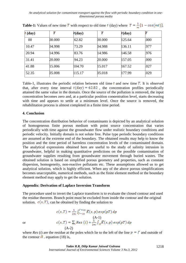
Table-1: Values of new time with respect to old time (day) where .
(day) (day) (day)
00 00.000 62.82 00.000 125.64 00.000
10.47 04.998 73.29 04.988 136.11 04.977
20.94 14.996 83.76 14.986 146.58 14.976
31.41 20.000 94.23 20.000 157.05 20.000
41.88 15.006 104.70 15.017 167.52 15.027
52.35 05.008 115.17 05.018 177.99 05.029
Table-1, illustrates the periodic relation between old time and new time . It is observed
that, after every time interval , the concentration profiles periodically
attained the same value in the domain. Once the source of the pollution is removed, the input
concentration becomes zero and, at a particular position concentration level, starts decreasing
with time and appears to settle at a minimum level. Once the source is removed, the
rehabilitation process is almost completed in a finite time period.
4. Conclusion
The concentration distribution behavior of contaminants is depicted by an analytical solution
of homogeneous finite porous medium with point source concentration that varies
periodically with time against the groundwater flow under realistic boundary conditions and
periodic velocity. Initially domain is not solute free. Pulse type periodic boundary conditions
are assumed at the extreme end of the boundary. The obtained results may help to know the
position and the time period of harmless concentration levels of the contaminated domain.
The analytical expressions obtained here are useful to the study of salinity intrusion in
groundwater, helpful in making quantitative predictions on the possible contamination of
groundwater supplies resulting from groundwater movement through buried wastes. The
obtained solution is based on simplified porous geometry and properties, such as constant
dispersion, homogeneity, non-reactive pollutants etc. These assumptions allowed us to get
analytical solution, which is highly efficient. When any of the above porous simplifications
becomes unacceptable, numerical methods, such as the finite element method or the boundary
element method may apply to get the solution.
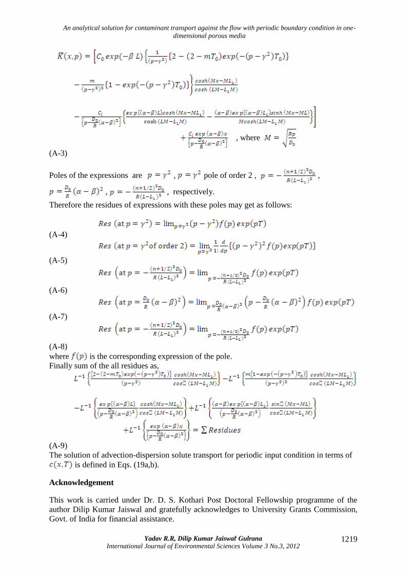
Appendix: Derivation of Laplace Inversion Transform
The procedure used to invert the Laplace transform is to evaluate the closed contour and used
the residue theorem. Branch point must be excluded from inside the contour and the original
solution. , can be obtained by finding the solution to
(A-1)
or
(A-2)
where Res (i) are the residue at the poles which lie to the left of the line and outside of
the contour . equation (18) is,
An analytical solution for contaminant transport against the flow with periodic boundary condition in one-
dimensional porous media
Yadav R.R, Dilip Kumar Jaiswal, Gulrana
International Journal of Environmental Sciences Volume 3 No.3, 2012 1219
, where
(A-3)
Poles of the expressions are , pole of order 2 , ,
, , respectively.
Therefore the residues of expressions with these poles may get as follows:
(A-4)
(A-5)
(A-6)
(A-7)
(A-8)
where is the corresponding expression of the pole.
Finally sum of the all residues as,
(A-9)
The solution of advection-dispersion solute transport for periodic input condition in terms of
is defined in Eqs. (19a,b).
Acknowledgement
This work is carried under Dr. D. S. Kothari Post Doctoral Fellowship programme of the
author Dilip Kumar Jaiswal and gratefully acknowledges to University Grants Commission,
Govt. of India for financial assistance.

An analytical solution for contaminant transport against the flow with periodic boundary condition in one-
dimensional porous media
Yadav R.R, Dilip Kumar Jaiswal, Gulrana
International Journal of Environmental Sciences Volume 3 No.3, 2012 1220
5. References
1. Andricˇevic´ R. and Cvetkovic´ V., (1998), Relative dispersion for solute flux in
aquifers. Journal of Fluid Mechanic., 361, pp 145-174.
2. 2Ataie-Ashtiani B., (1998), Contaminant transport in coastal aquifers, Ph.D. Thesis,
Department of Civil Eng. University of Queenland, Australia.
3. Bear J., (1972), Dynamics of Fluid in Porous Media, Elsvier Publ. Co. New York.
4. Bowden K. F., (1965), Horizontal mixing in the sea due to a shearing current, Journal
of Fluid Mechanics, 21, 83-95.
5. Caro C. G., 1966: The dispersion of indicator flowing through simplified models of
the circulation and its relevance to velocity profile in blood vessels, J. Physiol.,185,
pp.501-519.
6. Crank J., 1975: The Mathematics of Diffusion, Oxford Univ. Press, London, 2nd Ed.
7. Custodio E., (1988), Present state of coastal aquifer modelling: Short review. In:
Custodio E. Gurgui A., Lobo Ferreira J.P. (Eds.), Groundwater Flow and Quality
Modelling, NATO ASI Series, 224,Reidel, Dordrecht, pp 785–810.
8. Fang C.S., Wang S.N., Harrison W., (1972), Groundwater flow in a sandy tidal beach:
two-dimensional finite element analysis, Water Resources Research, 8, pp 121-128.
9. Frind E.O., (1982), Simulation of long-term transient density dependent transport in
groundwater, Advances in Water Resource, 5, pp.73-88.
10. Gelhar L. W. and Collins M. A., (1971), General analysis of longitudinal dispersion
in non-uniform flow, Water Resources Research, 7, pp.1511- 1521.
11. Hoopes J. A. and Harleman D.R.F., (1967), Wastewater recharge and dispersion in
porous media, Journal of Hydraulic Division (Am. Soc. Eng.), 93(HY5), pp 51-71.
12. Jeng D.S., Li L., Barry D.A., (2002), Analytical solution for tidal propagation in a
coupled semi-confined/phreatic coastal aquifer, Advances in Water Resource, 25(5),
pp 586–588.
13. Jaiswal D.K., Kumar A., Kumar N. and Yadava R. R., (2009), Analytical solutions
for temporally and spatially dependent solute dispersion of pulse type input
concentration in one dimensional semi-infinite media, Journal of Hydro-environment
Research, 2, pp 254-263.
14. Krabbenhoft D.P. and Webster K.E., (1995), Transient hydrological controls on the
chemistry of a seepage lake, Water Resources Research, 31(9), pp 2295-2305.
15. Kumar N., (1983), Dispersion of pollutants in semi-infinite porous media with
unsteady velocity distribution, Nordic Hydrology, pp 167-187.

An analytical solution for contaminant transport against the flow with periodic boundary condition in one-
dimensional porous media
Yadav R.R, Dilip Kumar Jaiswal, Gulrana
International Journal of Environmental Sciences Volume 3 No.3, 2012 1221
16. Kumar A., Jaiswal D.K. and Kumar N., (2010), Analytical solutions to one-
dimensional advection-diffusion with variable coefficients in semi-infinite media,
Journal of Hydrology, 380(3-4), pp 330-337.
17. 17. Li L., Barry D.A., Stagnitti F.and Parlange J.Y., (1999), Submarine
groundwater discharge and associated chemical input to a coastal sea, Water
Resources Research, 35(11), pp 3253-3259.
18. Li L., Barry D.A., Stagnitti F., and Parlange J.Y., (1999a), Tidal along-shore
groundwater flow in a coastal aquifer, Environmental Modeling Assessment, 4, pp
179-188.
19. Li L., Barry D.A., Jeng D.S., (2001), Tidal fluctuations in a leaky confined aquifer:
dynamic effects of an overlying phreatic aquifer, Water Resources Research, 37, pp
1095-1098.
20. Logan J. D. and Zlotnik V., (1995), The convection–diffusion equation with periodic
boundary conditions, Applied Mathematics Letter, 8(3), pp 55-61.
21. Masciopinto C., (2006), Simulation of coastal groundwater remediation: the case of
Nardo` fractured aquifer in Southern Italy, Environmental Modelling and Software,
21(1), pp 85-97.
22. Ogata A., and Bank R. B., (1961), A solution of differential equation of longitudinal
dispersion in porous media, U.S Geological survey professional paper, 411, A1-A7.
23. Purnalna A., Al-Barwani H.H., Al-Lawatia,M., 2003: Modelling dispersion of brine
waste discharges from a coastal desalination plant, Desalination 155, pp. 41-47.
24. Robinson M.A., Gallagher D.L., Reay W.G., (1998), Field observations of tidal and
seasonal variations in ground water discharge to estuarine surface waters, Ground
Water Monitoring and Remediation, 18 (1), pp 83–92.
25. Song, Z., Li, L., Kong, J. and Zhang, H. (2007), A new analytical solution of tidal
water table fluctuations in a coastal unconfined aquifer. Journal of Hydrology, 340,
pp 256-260.
26. Todd, D. K. (1980), Groundwater Hydrology. John Wiley, N.Y., 2nd Ed.
27. Townley, L.R. (1993) AQUIFEM-P: A periodic finite element aquifer flow model.
Users manual and description. Version 1.0, CSIRO Institute of Natural Resources and
Environment. Division of Water Resources, Technical Memorandum 93/13.
28. Townley, L.R. (1995), The response of aquifers to periodic forcing. Advances in
Water Resources, 18(30), pp 125-146.
29. Volker, R.E., Rushton, K.R. (1982), An assessment of the importance of some
parameters for sea water intrusion in aquifers and a comparison of dispersive
and sharp interface modeling approaches. Journal of Hydrology, 56, pp. 239-250.
30. Watson, E. J. (1983), Diffusion in oscillatory pipe flow. Journal of Fluid Mechanics,
133, pp 233-244.
An analytical solution for contaminant transport against the flow with periodic boundary condition in one-
dimensional porous media
Yadav R.R, Dilip Kumar Jaiswal, Gulrana
International Journal of Environmental Sciences Volume 3 No.3, 2012 1222
31. Yadav, R. R., Jaiswal D. K., Yadav, H. K. and Gulrana (2010), One-Dimensional
Temporally Dependent Advection Dispersion Equation In Porous Media: Analytical
Solution. Natural Resources Modeling, 23(4), pp 521-539.
32. Yim, C.S. and M.F.N. Mohsen (1992), Simulation of tidal effects on contaminant
transport in porous media, Ground Water, 30(1), pp. 78-86.