exact analytical solutions for contaminant transport … · exact analytical solutions for...

J. Hydrol. Hydromech., 61, 2013, 2, 146–160 DOI: 10.2478/johh-2013-0020

146

Exact analytical solutions for contaminant transport in rivers 1. The equilibrium advection-dispersion equation Martinus Th. van Genuchten 1 *, Feike J. Leij 2, Todd H. Skaggs 3, Nobuo Toride 4, Scott A. Bradford 3, Elizabeth M. Pontedeiro 5

1 Department of Mechanical Engineering, Federal University of Rio de Janeiro, UFRJ, Rio de Janeiro, RJ, Brazil. 2 Department of Civil and Construction Engineering Management, California State University, Long Beach, California, USA. 3 U.S. Salinity Laboratory, USDA, ARS, Riverside, California, USA. 4 Faculty of Bioresources, Mie University, Tsu, Japan. 5 Department of Nuclear Engineering, Federal University of Rio de Janeiro, UFRJ, Rio de Janeiro, RJ, Brazil. * Corresponding author. E-mail: [email protected]

Abstract: Analytical solutions of the advection-dispersion equation and related models are indispensable for predicting or analyzing contaminant transport processes in streams and rivers, as well as in other surface water bodies. Many useful analytical solutions originated in disciplines other than surface-water hydrology, are scattered across the literature, and not always well known. In this two-part series we provide a discussion of the advection-dispersion equation and related models for predicting concentration distributions as a function of time and distance, and compile in one place a large number of analytical solutions. In the current part 1 we present a series of one- and multi-dimensional solutions of the standard equilibrium advection-dispersion equation with and without terms accounting for zero-order production and first-order decay. The solutions may prove useful for simplified analyses of contaminant transport in surface water, and for mathematical verification of more comprehensive numerical transport models. Part 2 provides solutions for advec-tive-dispersive transport with mass exchange into dead zones, diffusion in hyporheic zones, and consecutive decay chain reactions. Keywords: Contaminant transport; Analytical solutions; Surface water; Advection-dispersion equation.

INTRODUCTION

Mathematical models have long proved useful for analyzing or predicting the fate and transport of contaminants in streams and rivers (Bencala, 1983; Fischer et al., 1979; Runkel, 1998; Thomann, 1973), including contaminant exchange with fluvial sediments and the surrounding stream bed (Thackston and Schnelle, 1970; Bencala and Walters, 1983; Wörman, 1998; Anderson and Phanikumar, 2011), often referred to as the hyporheic zone (Wörman, 1998; Runkel et al., 2003; Bencala, 2005; Gerecht et al., 2011). Such models may be used also for subsurface streams and karst systems (Field, 1997). Constitu-ents in surface waters may involve a range of specific natural and anthropogenic chemicals, including toxic trace elements, radionuclides, industrial solvents, pesticides, nutrients, patho-genic microorganisms, pharmaceuticals, and a variety of water quality variables such as total salinity or dissolved oxygen. Because of the many complex and often nonlinear physical, chemical and biological processes affecting contaminant transport in streams and rivers, numerical models are now increasingly used for prediction purposes (e.g., Anderson and Phanikumar, 2011; O’Connor et al., 2009; Runkel, 1998; Runkel and Chapra, 1993). Still, analytical and quasi-analytical approaches are useful for simplified analyses of a variety of contaminant transport scenarios, especially for relatively long spatial and time scales, when insufficient data are available to warrant the use of a comprehensive numerical model, and for testing numerical models. The application of analytical ap-proaches is greatly facilitated now also by mathematical soft-ware such as Maple, Mathematica and Matlab.

Although the literature contains many analytical solutions that are applicable to transport in rivers and streams, most of the solutions originated in other disciplines using mathematical-ly equivalent equations, and hence their existence may not be

familiar to many in the surface-water hydrology community (e.g. De Smedt et al., 2006; Huang, 2006). In this two-part series we assembled a large number of one- and multi-dimensional solutions for contaminant transport in streams and rivers. The solutions are for one-dimensional advective-dispersive transport, longitudinal transport and lateral disper-sion, transport with simultaneous first-order exchange with relative immobile or stagnant water zones (transient storage models), advective-dispersive transport with simultaneous diffusion into and out of hyporheic zones, and transport of solutes subject to consecutive decay chain reactions. Most of the solutions were derived from solutions to mathematically very similar problems in subsurface contaminant transport, on which the authors have worked for many years (e.g., Leij et al., 1991, Toride et al., 1993a, 1999; van Genuchten, 1981). Except for solutions pertaining to diffusion in hyporheic zones as pre-sented in part 2 (van Genuchten et al., 2013), most or all mod-els have been incorporated in the public-domain windows-based STANMOD software package (Šimůnek et al., 2000). In this part 1 we first start with a brief introduction of the advec-tion-dispersion equation governing transport in surface water bodies, applicable initial and boundary conditions, and a brief overview of analytical solution techniques. GOVERNING TRANSPORT EQUATION Formulation of the Advection-Dispersion equation

The transport of contaminants in surface and subsurface wa-ters is generally described with the Advection-Dispersion Equa-tion (ADE), or appropriate modifications or extensions thereof. The ADE distinguishes two transport modes: advective transport as a result of passive movement along with water, and dispersive/diffusive transport to account for diffusion and small-scale variations in the flow velocity as well as any other

2405

Exact analytical solutions for contaminant transport in rivers. 1. The equilibrium advection-dispersion equation

147

processes that contribute to solute spreading. Solute spreading is generally considered to be a Fickian or Gaussian diffu-sion/dispersion process. A considerable body of literature on dispersion processes now exists for both surface and subsurface contaminant transport (e.g., Bear and Verruijt, 1987; Fischer et al., 1979; Jury and Horton, 2004).

For one-dimensional transport, the solute flux Js (ML-2T-1) can be written as

Js = uC − Dx

∂C∂x

, (1)

where u is the longitudinal fluid flow velocity (LT-1), C is the solute concentration expressed as mass per unit volume of water (ML-3), Dx is the longitudinal dispersion coefficient ac-counting for the combined effects of ionic or molecular diffu-sion and hydrodynamic dispersion (L-2T-1), and x is the longitu-dinal coordinate (L).

The mass balance equation can be formulated in a general manner by considering the accumulation or depletion of solute in a control volume over time as a result of the divergence of the flux (i.e., net inflow or outflow), possible reactions, and the injection or extraction of solute along with the fluid phase:

∂C∂t

= −∇⋅ Js − Rs +RwCe , (2)

where t is time (T), and Rs represents arbitrary sinks (< 0) or sources (> 0) of solute (ML-3T-1), while the last term denotes injection (> 0) or pumping (< 0) of water with constituent con-centration Ce at a rate Rw (L3L-3T-1).

The use of analytical methods requires that some of the un-derlying processes affecting transport are simplified or approx-imated. Such simplifications include the use of constant values for u and Dx with respect to time and position, adopting ideal-ized initial and boundary conditions, assuming that production and degradation are limited to zero- or first-order processes, and describing solute sorption by fluvial sediments using a linear equilibrium isotherm (or neglecting sorption altogether). If the last two terms of the mass balance equation are ignored, substitution of the advective-dispersive flux, Js, yields the popularly used advection-dispersion equation (ADE) for one-dimensional transport as follows

∂C∂t

= Dx∂2C

∂x2 − u ∂C∂x

. (3)

A variety of solute source or sink terms may need to be im-

plemented in the ADE. One possible process during transport in rivers is sorption of contaminants on sediment along the main channel. The source/sink term for sorption may then be written as (e.g., Bencala, 1983)

Rs = sρ

∂S∂t

, (4)

where S is the sorbed concentration expressed as mass of solute per mass of sediment readily accessible for sorption (MM-1), and ρs is the mass of sediment per unit volume of river water (ML-3). For binary exchange in a system with a constant total solute concentration, linear equilibrium exchange is given by

S = KdC (5) in which the distribution coefficient Kd (L3M-1) may be viewed as the ratio of the sorbed (sediment) concentration and the dissolved (stream) concentration at equilibrium (Bencala et al., 1983). Substituting (1), (4) and (5) into (2) allows the ADE to be formulated in terms of one dependent variable (i.e., the stream solute concentration) according to

R ∂C∂t

= Dx ∂2C

∂x2 − u∂C∂x

(6)

in which the retardation factor R is given by

R = 1+ ρsKd . (7)

Sorption onto the sediments reduces the apparent advective and dispersive fluxes by a factor equal to R. This sorption is often considered negligible, in which case Kd = 0 and the value for R becomes equal to one. Analytical expressions for the concentration can generally be obtained only for linear sorp-tion. Because the mathematical problem is trivial with regard to the value for R (the values of time t in the analytical solutions are to be divided by R), sorption will not be considered explicit-ly in the remainder of our study.

Many other processes such as biodegradation or inactivation, radioactive decay, and production may affect the contaminant concentration. They can all be included in the sink/source term, Rs , in Eq. (2). The transport problem can still be solved analyti-cally if this term is described in terms of linear processes. For example, for relatively simple transport scenario's involving one or several sets of zero- and first-order rate expressions, the governing equation can always be represented in the form:

∂C∂t

= Dx ∂2C

∂x2 − u ∂C∂x

− µC + γ , (8)

where µ is a general first-order decay rate (T-1) and γ a zero-order production term (ML-3T-1). We assume in this study that µ and γ are either zero or always positive. Additional processes such as nonlinear exchange, precipitation/dissolution, and sorp-tion or chelation of constituents by moving sediment, are not considered here since the resulting transport problem generally will require numerical solution techniques. Concentration modes and boundary conditions

The mathematical solution of Eq. (8) and related transport equations requires auxiliary conditions specifying the initial and boundary condition of the transport problem. It is important that the boundary conditions accurately describe the adopted modes of solute injection and detection. Concentrations are usually expressed in terms of the amount of solute per unit volume of water. Although the microscopic concentration is based on an infinitesimally small liquid volume, for practical purposes a much larger finite averaging scale must be used. In this way a macroscopic volume-averaged or resident concentra-tion, CV, can be defined as

VC = 1

ΔV ∫ ∫ ∫ c dV , (9)

Martinus Th. van Genuchten, Feike J. Leij, Todd H. Skaggs, Nobuo Toride, Scott A. Bradford, Elizabeth M. Pontedeiro

148

where c is the local concentration (ML-3) in a microscopic volume element, V, and ΔV is the representative elementary volume (Bear and Verruijt, 1987). Spatial or temporal averages beyond the REV scale may also be employed (Leij and Toride, 1995). Unless stated otherwise, we will assume that all concen-trations are macroscopic and are of the volume-averaged or resident type.

Flux-averaged concentrations, CF, may arise when the con-centration is determined as the ratio of the solute flux, Js, and the water flux, u, passing through a given cross section during an arbitrary time interval (Kreft and Zuber, 1978; Parker and van Genuchten, 1984a), i.e.,

FC = Js / u. (10)

A relationship between the volume- and flux-averaged concen-trations can be established by substituting the one-dimensional advective-dispersive flux (Eq. (1)) into (10) to give

FC = VC − xDu

∂CV

∂x. (11)

Notice that CV and CF become similar for small values of Dx/u, i.e., when dispersion is negligible as compared to advection. We emphasize that CF is a mathematical entity that depends on the formulation of the contaminant flux. As will be discussed shortly, the selection of boundary conditions is related to the concentration mode.

The initial condition can be formulated as

C(x, 0) = f (x), (12) where f(x) is an arbitrary function versus distance, the simplest case being the situation where the stream has a constant (zero or positive) background concentration. An alternative initial condition, often assumed for one-dimensional stream transport, is the Dirac condition specifying instantaneous release of a prescribed mass. This relatively hypothetical condition assumes that a contaminant mass, m, can be distributed instantaneously over an infinitely small region, for example a thin plane of area A across the main channel at some longitudinal position xo , i.e.,

f (x) = m

Aδ (x − xo ), (13)

where δ(x–xo) is the Dirac function (L-1) having the property

-∞

∞∫ δ (x − xo )dx = 1

with δ (x − xo ) = 0 for all x ≠ xo .

(14)

Proper selection of boundary conditions is a somewhat eso-

teric topic that has received considerable attention in the litera-ture on transport in porous media (e.g., Batu et al., 2013; van Genuchten and Parker, 1984). Many transport problems involve the application of a solute with a concentration described by a spatially independent function, g(t), to a surface water body that, for modeling purposes, can have a finite, semi-infinite, or infinite length. The method of application (or the contaminant source) may also vary widely (pumping or spraying, line or point sources, continuous or finite pulse type applications).

Boundary conditions are simplest for transport problems de-fined over infinite domains (–∞ < x < ∞). To ensure that the concentration remains bounded, the inlet and outlet conditions can be written in the form

∂C∂x

( ±∞, t) = 0. (15)

Two types of conditions are often used at the inlet of semi-

infinite media (0 ≤ x ≤ ∞) or finite media (0 ≤ x ≤ L). These conditions are based on continuity of either the concentration or the solute flux across the inlet boundary. We do not discuss here the simultaneous use of both conditions since this situation is generally too complicated for deriving relatively simple analytical solutions.

First- or concentration-type inlet boundary conditions, also referred to as Dirichlet conditions, require the concentration to be continuous across the interface at all times, i.e.,

C(0,t) = g(t) t > 0. (16) The drawback of this condition is that the (macroscopic) con-centration at the interface just inside the river system will, in reality, not respond instantaneously to changes in the influent concentration. Condition (16) generally leads to discrepancies in the mass balance when considered over a finite or semi-infinite system (Batu and van Genuchten, 1990; Parker and van Genuchten, 1984a). Mass conservation can be ensured by using a third- or flux-type condition at the inlet (often referred to also as a Robin or Cauchy type condition):

x=0+uC − xD

∂C∂x

⎛⎝⎜

⎞⎠⎟

= ug(t), (17)

where 0+ indicates a position just inside the system being con-sidered. Analytical solutions for first-type conditions are gener-ally somewhat simpler than those for third-type inlet condi-tions. This probably explains the popularity of first-type condi-tions despite mass balance errors in the predicted resident con-centration distributions.

Some commonly-used functions for the influent concentra-tion, g(t), in (16) or (17) are the Dirac function, a finite square pulse, and a Heaviside or step function. An instantaneous appli-cation of a solute amount m at the inlet, x = 0, at an arbitrary time, to, across an area A is given by

g(t) = m

uAδ (t − to ), (18)

where δ(t–to) is the Dirac delta function in time (T-1). Instanta-neous release into a stream at x = 0 can be described alterna-tively also with a Dirac type initial condition.

The application of a finite pulse can be formulated as

g(t) =

Co 0 < t ≤ to

0 t > to

⎧⎨⎪

⎩⎪ (19)

where to is the time duration of the applied pulse having con-centration Co. Note that to approaches infinity for a single step change. Because of the linearity of the ADE, solutions for problems involving an arbitrary number of finite pulses of different durations (to) and strengths (Co) can be readily inferred


149

from the single step solution; the Heaviside function is conve-nient for this purpose.

The exit boundary condition can be defined in terms of a ze-ro gradient at a finite or infinite distance from the inlet, leading to the assumption of having a finite or semi-infinite medium, respectively. The infinite outlet condition is mathematically far more convenient than the finite condition, and hence has been far more popular in analytical transport studies, even when finite systems are simulated. The infinite outlet condition is given by

∂C∂x

(∞,t) = 0. (20)

The use of this condition for a finite system implies that a semi-infinite fictitious medium with identical properties is placed beyond the system of interest. No assumptions have to be made regarding the physical processes at the outlet, x = L, other than that the ADE is applicable just like everywhere else at x > 0.

The domain for most transport problems involving rivers is best described with a semi-infinite or infinite system, rather than a finite system. However, we shall provide in this paper also several analytical solutions for finite systems since numer-ical solutions, by their very nature, can be applied only to finite domains. Assuming that no dispersion occurs for x > L, the approximate condition for a finite system is

∂C∂x

(L,t) = 0. (21)

This conditions implies both flux and concentration continuity at the downstream boundary of the finite transport domain. A zero-gradient outlet condition is also appealing when no transport occurs across a boundary, such as is the case for so-lute diffusion or heat transport problems involving insulated media.

The choice of the boundary conditions is affected by the concentration mode (Kreft and Zuber, 1978). In practice only the dependency of the inlet condition is considered (cf. Parker and van Genuchten, 1984a). A typical problem in terms of the usual resident concentration can be formulated as

∂CV

∂t = xD

∂2CV

∂x2 − u ∂CV

∂x (22)

subject to a uniform initial condition

VC (x,0) = f (x) = Ci (23)

a third-type inlet boundary condition to avoid mass balance problems

x=0+

VuC − xD ∂CV

∂x

⎛

⎝⎜

⎞

⎠⎟ = ug(t) (24)

and a semi-infinite or finite outlet condition

∂CV

∂x(∞,t) = 0,

∂CV

∂x (L,t) = 0. (25a, b)

As shown by Parker and van Genuchten (1984b) this problem can be readily transformed to the flux-averaged mode using Eq. (11) to give

∂C F

∂t= xD

∂2C F

∂x2 − u∂C F

∂x (26)

subject to

FC (x,0) = Ci (27)

CF (0,t) = g(t), (28)

∂ FC∂x

(∞,t) = 0 or

∂C F

∂x (L,t) = −

Dxu

∂2CV

∂x2(L,t).

(29)

Notice that the mathematical problem in terms of CF involves the simpler first-type inlet condition with mass now being con-served, unlike the use of a first-type condition for transport problems in terms of CV. This shows that solutions for a semi-infinite system involving a first-type inlet condition represent mass-conserving solutions if the concentration, inside and outside the solution domain, is interpreted as being of the flux-averaged type (Batu et al., 2013; Parker and van Genuchten, 1984a). The transformations leading to Eqs (26) through (29) are less convenient for finite systems as well as for semi-infinite systems having nonuniform initial conditions (Toride et al., 1993b).

Differences between the preferred third-type and first-type solutions for CV are usually minor except for small values of the dimensionless distance (ux/Dx) and time (u2t/Dx) (e.g., van Genuchten and Parker, 1984). Since advective transport usually dominates dispersive transport in rivers and streams, the selec-tion of a first- or third-type condition is of secondary im-portance for most practical river transport problems, except near the inlet. However, the issue should not be overlooked for code verification when small errors in the mass balance are important. Hence, analytical solutions will be presented for both first- and third-type inlet conditions. All concentrations in this study are understood to be of the resident type; flux-averaged concentrations can be derived as needed from the resident solutions using Eq. (11). SOLUTION TECHNIQUES Problems in one dimension

Before presenting specific analytical solutions, two different solution techniques will be briefly reviewed. Although a wide variety of solution procedures can be followed, many linear transport problems can be solved by either using a transfor-mation of variables, or implementing Laplace transforms.

Most streams can be considered infinite systems in the longi-tudinal direction. This makes them quite suitable for making a transformation of variables to cast the ADE in a simpler form. For example, the coordinate transformation

ξ = x − utτ = t

(30)


150

transforms Eq. (3) subject to

C(x,0) =

Co x < 00 x > 0

⎧⎨⎪

⎩⎪

∂C∂x

(±∞,t) = 0 (31)

into the heat transfer (or solute diffusion) problem

∂C∂τ

= Dx∂2C

∂ 2ξ (32)

C(ξ ,0) =

Co ξ < 00 ξ > 0

⎧⎨⎪

⎩⎪ (33)

Analytical solutions for this and many related problems have been widely reported in the literature (e.g. Carslaw and Jaeger, 1959; Crank, 1975).

An alternative transformation

ξ = x − ut

4Dxt (34)

allows the ADE to be written as

2d Cd 2ξ

+ 2ξ dCdξ

= 0, (35)

C(ξ ) =

Co ξ < −∞

0 ξ > ∞

⎧⎨⎪

⎩⎪ (36)

This ordinary differential equation can be solved through a reduction of order according to

dψdξ

+ 2ξψ = 0 where ψ = dCdξ

. (37)

Separation of variables and integration leads to the following solution of (37):

ψ =α1exp(−ξ 2 ), (38) where α1 is an integration constant. Integration of ψ between ξ (corresponding to the desired concentration, C), and ∞, and making use of a zero-concentration as dictated by the infinite boundary condition, leads to

C =ξ

∞∫ α1exp(−w2 )dw+α2 =

π2

α1erfc x − ut

4Dxt

⎛

⎝⎜⎜

⎞

⎠⎟⎟+α2 (39)

in which w is a dummy integration variable, α2 is an additional integration constant, and erfc represents the complementary error function (e.g., Gautschi, 1964). The boundary conditions are used to evaluate α1 and α2. The final solution is

C =Co2

erfc x − ut

4Dxt

⎡

⎣⎢⎢

⎤

⎦⎥⎥. (40)

More complicated transformations were previously used by Brenner (1962) and Selim and Mansell (1976); several can also be found in Zwillinger (1989).

The complementary error function (erfc) in Eq. (40) fre-quently occurs in analytical solutions of the ADE. Several approximations can be found in Gautschi (1964). Its evaluation is sometimes not straightforward, especially when erfc occurs in combination with the exponential function and either or both of these functions have unusually large or small arguments. A useful routine for evaluating erfc is listed in van Genuchten and Alves (1982). In some cases, especially for situations with exponentially decaying inflow concentrations, the argument of the erfc function and other terms in the analytical solutions may involve complex variables with real and imaginary parts. An accurate subroutine for such cases is given by van Genuchten (1985b).

Linear partial differential equations are often solved with in-tegral transforms. The transformations generally lead to ordi-nary differential or even algebraic equations which are much easier to solve than the original partial differential equations. Subsequent inversion of the solution to the regular space-time domain is generally the most complicated part of the solution procedure. The inversion often can be accomplished in several ways (cf. Özişik, 1989; Pérez-Guerrero et al., 2009; Sneddon, 1995; Spiegel, 1965). Laplace transforms traditionally have been the most popular for solving the ADE (Leij et al., 1993; Toride et al., 1993a; van Genuchten, 1981). Problems in several dimensions

Solutions of transport problems in two and three dimensions are in many cases a direct extension of the one-dimensional solutions. We consider here three-dimensional problems in Cartesian coordinates (x,y,z) with uniform flow and dispersion in the longitudinal direction and dispersion in the transverse direction. We note that solutions for two-dimensional problems follow directly from solution of the more general three-dimensional examples.

The three-dimensional form of the ADE is given by

∂C∂t

= Dx∂2C

∂x2 − u∂C∂x

+ Dy ∂2C

∂y2 + Dz∂2C

∂z2 , (41)

where Dy and Dz are dispersion coefficients (L2T-1) in the trans-verse y and z directions. Although the boundary conditions may vary depending upon the assumed geometry of the system, they normally include zero-gradient conditions at the transverse boundaries. Below are the conditions for a somewhat idealized three-dimensional system involving a semi-infinite longitudinal direction and two infinite transverse directions:

C(x, y,z,0) = f (x, y,z), (42)

x=0+C −ω xD

u∂C∂x

⎛⎝⎜

⎞⎠⎟

= g( y,z,t) ω = 0,1, (43)

∂C∂x

(∞, y,z,t) = 0, (44)


151

C(x,±∞,z,t) = 0

∂C∂y

(x,±∞, z, t) = 0, (45)

C(x, y,±∞,t) = 0

∂C∂z

(x, y,±∞,t) = 0, (46)

where ω equals 0 or 1 for a first- and third-type boundary con-dition, respectively. Note that f(x,y,z) and g(y,z,t) are arbitrary initial and influent distributions, respectively. These functions can be specified in a similar manner as for the one-dimensional case except that f and g now depend on multiple coordinates instead of one.

For three-dimensional infinite systems the use of a moving longitudinal coordinate (Eq. (30)) readily transforms the ADE and its auxiliary conditions into a three-dimensional diffusion problem for which a wealth of analytical solutions exist. An-other straightforward method of solving multidimensional transport problems is the use of the product rule which states that the product of the solutions of (simpler) one-dimensional problems may directly give the desired three-dimensional solu-tion (e.g., Carslaw and Jaeger, 1959). Consider the three one-dimensional problems

∂Cx∂t

= Dx∂2Cx

∂x2 − u∂Cx∂x

, (47)

∂Cy

∂t= Dy

∂2Cy

∂y2 , (48)

∂Cz∂t

= Dz∂2Cz

∂z2 . (49)

The product of the solutions of these three one-dimensional problems, i.e.,

C(x, y,z,t) = Cx (x,t) Cy ( y,t) Cz (z,t) (50)

also satisfies the three-dimensional transport equation. Applica-tion of the product rule requires that the boundary conditions be homogeneous and that the initial condition for the three-dimensional problem can be written as a product of the three one-dimensional initial conditions.

Several approaches, in addition to moving coordinate trans-formation and product rules, have been used in the literature. These include separation of variables and Fourier series (Bruch and Street, 1967), Green's functions (Leij and van Genuchten, 2000; Sagar, 1982; Yeh and Tsai, 1976), or integral transforms (Cleary, 1973; Leij and Dane, 1990; Leij et al., 1993, Pérez Guerrero et al., 2013).

For many river systems at least one direction will be finite, which may complicate the mathematical solutions. Several integral transforms, mostly of the Fourier type, have been used by Özişik (1989) and Sneddon (1995) for such situations. In some cases one or two of the finite directions can be neglected by using a depth-averaged concentration, or by making use of uniformity in the initial and boundary conditions across the stream. Another approach is the use of fictitious constituent sources outside the solution domain to ensure a zero-gradient at the boundaries (e.g., see p. 49 of Fischer et al., 1979). This

approach permits one to still use the relatively simple solutions available for infinite outlet conditions. SPECIFIC ADE SOLUTIONS One-dimensional solutions with third-type inlet condition

Consider the ADE for a contaminant subject to a combina-tion of first-order decay and zero-order production to represent a variety of physical, chemical or biological reactions:

∂C∂t

= Dx∂2C

∂x2 − u∂C∂x

− µC + γ . (51)

Eq. (51) will be solved for the following initial and boundary conditions:

C(x,0) = f (x), (52)

x=0+uC −ωDx

∂C∂x

⎛⎝⎜

⎞⎠⎟

= ug(t), (53)

∂C∂x

(∞,t) = 0 or ∂C∂x

(L,t) = 0. (54a, b)

Analytical solutions for a third-type inlet condition (ω = 1)

are given below under Case A, while those for a first-type inlet condition (ω = 0) are presented under Case B. The first solution will be for a Dirac delta type initial distribution, from which solutions for arbitrary initial profiles can be derived. The re-maining one-dimensional solutions were selected from van Genuchten (1981) and van Genuchten and Alves (1982). The latter publication contains a large number of solutions for situa-tions with and without zero-order production and first-order decay. Most of the semi-infinite solutions, as well as others, were later included in the CXTFIT computer programs (Parker and van Genuchten, 1984b; Toride et al., 1999), which later were incorporated into the windows-based STANMOD soft-ware package (Simůnek et al., 2000).

Case A0. Semi-infinite domain with zero initial concentra-tion and a Dirac-type input function g(t) = mδ(t)/Au. Neglecting any production or decay (µ = γ = 0), the solution is

C(x,t) = mA

1

πDxt exp − (x − ut)2

4Dxt

⎡

⎣⎢⎢

⎤

⎦⎥⎥

⎧⎨⎪

⎩⎪

− u2Dx

expuxDx

⎛

⎝⎜⎞

⎠⎟ erfc

x + ut

4Dxt

⎡

⎣⎢⎢

⎤

⎦⎥⎥

⎫⎬⎪

⎭⎪.

(55)

As mentioned previously, an alternative solution exists for a Dirac-type initial distribution in an infinite medium.

In case of an arbitrary input function, g(t), the expression for the concentration can be written as the convolution of the input signal and the concentration for the Dirac function:


152

C(x,t) = ug(t −τ ) 1

πDxτ exp − (x − uτ )2

4Dxτ⎡

⎣⎢⎢

⎤

⎦⎥⎥

⎧⎨⎪

⎩⎪0

t∫

− u2Dx

expuxDx

⎛

⎝⎜⎞

⎠⎟ erfc

x + uτ4Dxτ

⎡

⎣⎢⎢

⎤

⎦⎥⎥

⎫⎬⎪

⎭⎪dτ .

(56)

Fig. 1 shows an example of the Dirac solution given by Eq.

(55) using parameter values selected previously by De Smedt et al. (2005) to test their analytical solution for the same Dirac inlet problem but assuming a first-type boundary condition (the solution of which is given by Case B0 below). The example involves an instantaneous injection (or spill) of 1 kg of a solute in the main channel of a river having a cross-section of 10 m2, an average flow velocity of 1 m/s and a dispersion coefficient of 5 m2/s. De Smedt et al. (2005) in their analysis also included the effects of a dead storage zone which we ignore here (that case will be discussed in part 2). Fig. 1 shows the solute distri-butions in the stream after 500, 1000 and 1500 s. The curve for t = 1000 s is essentially the same as the one calculated by De Smedt et al. (2005) assuming no mass transfer into the dead zone (their Fig. 1 with α = 0).

Fig. 1. Calculated concentration distributions obtained with Eq. (55) for instantaneous injection of 1 kg of solute in a stream having a cross-sectional area of 10 m2 assuming a third-type Dirac input boundary condition (u = 1 m s-1, Dx = 5 m2 s-1). Case A1. Semi-infinite domain with uniform initial concentra-tion, f(x) = Ci and no production or decay. The inlet concentra-tion function, g(t), is of the pulse type (a Heaviside type func-tion) with constant concentration Co , i.e.,

g(t) =

Co 0 < t ≤ to

0 t > to.

⎧⎨⎪

⎩⎪ (57)

The solution of this example is

C(x,t) =Ci + (Co −Ci )A(x,t) 0 < t ≤ to

Ci + (Co −Ci )A(x,t)−Co A(x,t − to ) t > to ,

⎧⎨⎪

⎩⎪

(58)

where

A(x,t) = 12

erfc x − ut

4Dxt

⎡

⎣⎢⎢

⎤

⎦⎥⎥ + u2t

πDx exp −

(x − ut 2)4Dxt

⎡

⎣⎢⎢

⎤

⎦⎥⎥

− 12

1 + uxDx

+ u2tDx

⎛

⎝⎜

⎞

⎠⎟ exp

uxDx

⎛

⎝⎜⎞

⎠⎟ erfc

x + ut

4Dxt

⎡

⎣⎢⎢

⎤

⎦⎥⎥.

(59)

Here we illustrate one possible application of the above ana-

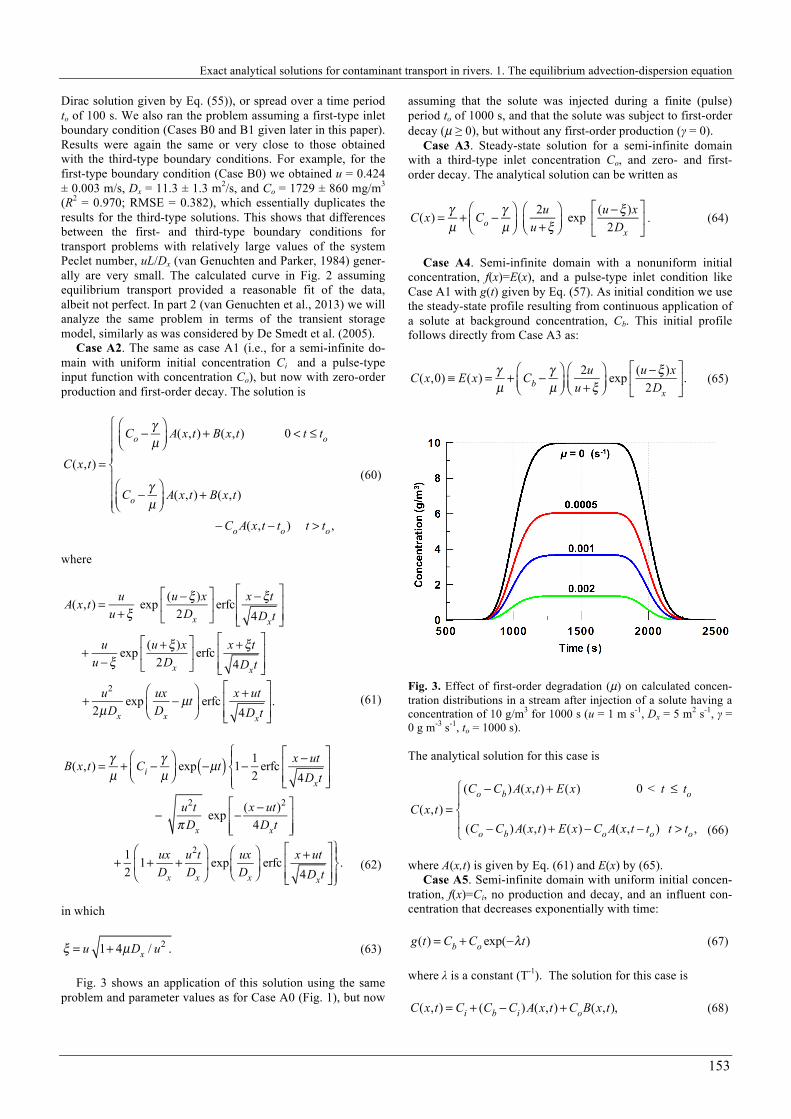
lytical solution by fitting the transport parameters in Eqs. (58) and (59) to observed data obtained by Brevis et al. (2001) as discussed by De Smedt et al. (2005). The data pertain to a tracer experiment in the Chillán River in Chile using a 20% Rhoda-mine WT solution injected simultaneously at multiple points along a lateral cross-section of the river at x = 0. Fig. 2 shows the observed data of one of their experiments (Exp. I-3), in this case for the application of 157.1 g of tracer at x = 0, with mea-surements made 4604 m downstream of the injection point. Because of the relative short duration of the experiments, pho-todegradation and sorption of Rhodamine WT were presumed to be negligible (De Smedt et al., 2005).

Fig. 2. Observed (solid squares) and fitted (continuous line) con-centrations for tracer experiment I-3 of Brevis et al. (2001) and De Smedt et al. (2005).

Fig. 2 shows the data along with the fitted curve based on Eqs (58) and (59). Parameters were estimated using the nonlin-ear least-squares optimization features of the CXTFIT code (Toride et al., 1999) within STANMOD. The code allows one to estimate not only the longitudinal flow velocity u and the longitudinal dispersion coefficient Dx, but also the concentra-tion Co of the applied tracer solution for a given value of the injection or pulse time to in Eq. (58). Assuming a very short injection period of only 10 s, we obtained the following param-eter values (with their 95% confidence intervals): u = 0.426 ± 0.003 m/s, Dx = 11.4 ± 1.4 m2/s, and Co = 1729 ± 86 mg/m3. The coefficient of determination (R2) of the fit was 0.983, and the root mean square error (RMSE) 0.382 mg/m3). One may verify that the total amount of solute mass (m) injected per m2 cross-sectional area hence equals m = u Co

to, or 7.37 g/m2. Given that a total amount of 157.1 g of tracer was applied to the river, this translates to an effective cross-sectional area of 157.1 g/7.37 (g/m2) or 21.3 m2 of the channel as calculated with the equilibrium ADE transport model.

The above calculations assume applicability of Eqs. (58) and (59) using a solute injection pulse of 10 s. Exactly the same results were obtained when the total mass was assumed to be applied instantaneously (as estimated with CXTFIT using the

5000 7500 10000 12500 15000 17500 200000

1

2

3

4

5

6

7C

once

ntra

tion

(mg/

m3 )

Time (s)


153

Dirac solution given by Eq. (55)), or spread over a time period to of 100 s. We also ran the problem assuming a first-type inlet boundary condition (Cases B0 and B1 given later in this paper). Results were again the same or very close to those obtained with the third-type boundary conditions. For example, for the first-type boundary condition (Case B0) we obtained u = 0.424 ± 0.003 m/s, Dx = 11.3 ± 1.3 m2/s, and Co = 1729 ± 860 mg/m3 (R2 = 0.970; RMSE = 0.382), which essentially duplicates the results for the third-type solutions. This shows that differences between the first- and third-type boundary conditions for transport problems with relatively large values of the system Peclet number, uL/Dx (van Genuchten and Parker, 1984) gener-ally are very small. The calculated curve in Fig. 2 assuming equilibrium transport provided a reasonable fit of the data, albeit not perfect. In part 2 (van Genuchten et al., 2013) we will analyze the same problem in terms of the transient storage model, similarly as was considered by De Smedt et al. (2005).

Case A2. The same as case A1 (i.e., for a semi-infinite do-main with uniform initial concentration Ci and a pulse-type input function with concentration Co), but now with zero-order production and first-order decay. The solution is

C(x,t) =

Co −γµ

⎛⎝⎜

⎞⎠⎟

A(x,t)+ B(x,t) 0 < t ≤ to

Co −γµ

⎛⎝⎜

⎞⎠⎟

A(x,t)+ B(x,t)

⎧

⎨

⎪⎪⎪

⎩

⎪⎪⎪

−Co A(x,t − to ) t > to ,

(60)

where

A(x,t) = uu +ξ

exp (u −ξ )x

2Dx

⎡

⎣⎢

⎤

⎦⎥ erfc

x −ξt

4Dxt

⎡

⎣⎢⎢

⎤

⎦⎥⎥

+ u

u −ξ exp

(u +ξ )x2Dx

⎡

⎣⎢

⎤

⎦⎥ erfc

x +ξt

4Dxt

⎡

⎣⎢⎢

⎤

⎦⎥⎥

+ u2

2µDx exp

uxDx

− µt⎛

⎝⎜⎞

⎠⎟ erfc

x + ut

4Dxt

⎡

⎣⎢⎢

⎤

⎦⎥⎥.

(61)

B(x,t) = γµ+ Ci −

γµ

⎛⎝⎜

⎞⎠⎟ exp −µt( ) 1− 1

2erfc

x − ut

4Dxt

⎡

⎣⎢⎢

⎤

⎦⎥⎥

⎧⎨⎪

⎩⎪

− u2tπDx

exp − (x − ut)2

4Dxt

⎡

⎣⎢⎢

⎤

⎦⎥⎥

+ 12

1+ uxDx

+ u2tDx

⎛

⎝⎜

⎞

⎠⎟ exp

uxDx

⎛

⎝⎜⎞

⎠⎟ erfc

x + ut

4Dxt

⎡

⎣⎢⎢

⎤

⎦⎥⎥

⎫⎬⎪

⎭⎪.

(62)

in which

ξ = u 1+ 4µDx / u2 . (63)

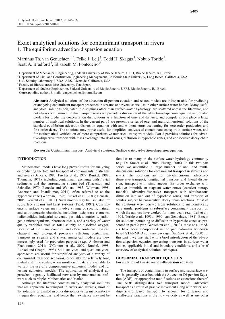
Fig. 3 shows an application of this solution using the same problem and parameter values as for Case A0 (Fig. 1), but now

assuming that the solute was injected during a finite (pulse) period to of 1000 s, and that the solute was subject to first-order decay (µ ≥ 0), but without any first-order production (γ = 0).

Case A3. Steady-state solution for a semi-infinite domain with a third-type inlet concentration Co, and zero- and first-order decay. The analytical solution can be written as

C(x) = γ

µ+ Co −

γµ

⎛⎝⎜

⎞⎠⎟

2uu +ξ

⎛⎝⎜

⎞⎠⎟ exp

(u −ξ )x2Dx

⎡

⎣⎢

⎤

⎦⎥ . (64)

Case A4. Semi-infinite domain with a nonuniform initial

concentration, f(x)=E(x), and a pulse-type inlet condition like Case A1 with g(t) given by Eq. (57). As initial condition we use the steady-state profile resulting from continuous application of a solute at background concentration, Cb. This initial profile follows directly from Case A3 as:

C(x,0) ≡ E(x) = γ

µ+ Cb −

γµ

⎛⎝⎜

⎞⎠⎟

2uu +ξ

⎛⎝⎜

⎞⎠⎟ exp

(u −ξ )x2Dx

⎡

⎣⎢

⎤

⎦⎥. (65)

Fig. 3. Effect of first-order degradation (µ) on calculated concen-tration distributions in a stream after injection of a solute having a concentration of 10 g/m3 for 1000 s (u = 1 m s-1, Dx = 5 m2 s-1, γ = 0 g m-3 s-1, to = 1000 s). The analytical solution for this case is

C(x,t) =(Co −Cb)A(x,t)+ E(x) 0 < t ≤ to

(Co −Cb)A(x,t)+ E(x)−Co A(x,t − to ) t > to ,

⎧

⎨⎪

⎩⎪

(66)

where A(x,t) is given by Eq. (61) and E(x) by (65).

Case A5. Semi-infinite domain with uniform initial concen-tration, f(x)=Ci, no production and decay, and an influent con-centration that decreases exponentially with time:

g(t) = Cb +Co exp(−λt) (67) where λ is a constant (T-1). The solution for this case is

C(x,t) = Ci + (Cb −Ci )A(x,t)+CoB(x,t), (68)


154

where

A(x,t) = 12

erfc x − ut

4Dxt

⎡

⎣⎢⎢

⎤

⎦⎥⎥ +

u2tπDx

exp − (x − ut)2

4Dxt

⎡

⎣⎢⎢

⎤

⎦⎥⎥

− 12

1+ uxDx

+ u2tDx

⎛

⎝⎜

⎞

⎠⎟ exp

uxDx

⎛

⎝⎜⎞

⎠⎟ erfc

x + ut

4Dxt

⎡

⎣⎢⎢

⎤

⎦⎥⎥.

(69)

B(x,t) = exp(−λt)u

u +κ exp

(u −κ )x2Dx

⎛

⎝⎜⎞

⎠⎟ erfc

x −κ t

4Dxt

⎡

⎣⎢⎢

⎤

⎦⎥⎥

⎧⎨⎪

⎩⎪

+ uu −κ

exp(u +κ )x

2Dx

⎛

⎝⎜⎞

⎠⎟erfc

x +κ t

4Dxt

⎡

⎣⎢⎢

⎤

⎦⎥⎥

⎫⎬⎪

⎭⎪

− u2

2λDx exp

uxDx

⎛

⎝⎜⎞

⎠⎟ erfc

x + ut

4Dxt

⎡

⎣⎢⎢

⎤

⎦⎥⎥

(70)

and

κ = u 1− 4λDx / u2 . (71) Note that this example reduces to Case A1 (only for t < to) when Co = 0.

Case A6. Finite domain with zero initial concentration, f(x) = 0, a third-type inlet condition, and no zero- and first-order rate processes (i.e., µ = γ = 0). The inlet condition is again the same as for Case A1, i.e., a pulse type concentration with con-stant Co. The outlet condition is now a zero gradient at x = L as given by Eq. (21). The solution for this case is (Brenner, 1962):

C(x,t)Co

= 1− 2uLDx m−1

∞∑

G(x)expux

2Dx− u2t

4Dx+βm

2 Dxt

L2

⎡

⎣⎢⎢

⎤

⎦⎥⎥

βm2 + uL

2Dx

⎛

⎝⎜⎞

⎠⎟

2

+ uLDx

⎡

⎣

⎢⎢

⎤

⎦

⎥⎥βm

2 + uL2Dx

⎛

⎝⎜⎞

⎠⎟

2⎡

⎣

⎢⎢

⎤

⎦

⎥⎥

, (72a)

where

G(x) = βm βm cos

βmxL

⎛⎝⎜

⎞⎠⎟+ uL

2Dxsin

βmxL

⎛⎝⎜

⎞⎠⎟

⎡

⎣⎢⎢

⎤

⎦⎥⎥

(72b)

in which the eigenvalues βm are the positive roots of

mβ cot( mβ )− m

2β Dx

uL+ uL

4Dx= 0. (73)

The above series solution converges very slowly when advec-tion dominates dispersion as is often the case for stream transport problems. For either

uLDx

> 5+ 40utL

or uLDx

>100 (74)

the following approximate solution may be used (Brenner, 1962; van Genuchten and Alves, 1982):

C(x,t)Co

= 12

erfc x − ut

4Dxt

⎡

⎣⎢⎢

⎤

⎦⎥⎥ + u2t

πDx exp −

2(x − ut)4Dxt

⎡

⎣⎢⎢

⎤

⎦⎥⎥

− 12

1+ uxDx

+ u2tDx

⎛

⎝⎜

⎞

⎠⎟ exp

uxDx

⎛

⎝⎜⎞

⎠⎟erfc

x + ut

4Dxt

⎡

⎣⎢⎢

⎤

⎦⎥⎥

+ 4u2tπDx

1+ u4Dx

(2L− x + ut)⎡

⎣⎢

⎤

⎦⎥ exp

uLDx

− (2L− x + ut)2

4Dxt

⎡

⎣⎢⎢

⎤

⎦⎥⎥

− uDx

2L− x + 3ut2

+ u4Dx

(2L− x + ut 2)⎡

⎣⎢

⎤

⎦⎥

⎧⎨⎪

⎩⎪

• exp uLDx

⎛

⎝⎜⎞

⎠⎟ erfc

(2L− x)+ ut

4Dxt

⎡

⎣⎢⎢

⎤

⎦⎥⎥

⎫⎬⎪

⎭⎪.

(75)

Although in most cases considerably more complicated, a

large number of analytical solutions are also available for finite systems with zero-order production and/or first order decay (Pérez Guerrero et al., 2009; van Genuchten and Alves, 1982). One-dimensional solutions with first-type inlet condition

Case B0. Semi-infinite domain with zero initial concentra-tion, a first-type (ω = 0) inlet condition, and a Dirac-type input concentration. The solution for the case of no production or decay is

C(x,t) = mAu

x

4πDxt3 exp − (x − ut)2

4Dxt

⎡

⎣⎢⎢

⎤

⎦⎥⎥. (76)

For arbitrary input profiles the expression for the concentration can again be written as the convolution of the input signal and the concentration for the Dirac input:

C(x,t) = xg(t −τ )

4πDxτ30

t∫ exp

(x − uτ )2

4Dxτ⎡

⎣⎢⎢

⎤

⎦⎥⎥

dτ . (77)

Case B1. Semi-infinite domain with uniform initial concen-

tration, f(x) = Ci, and a pulse-type solute application (i.e., Eq. (57) as for Case A1). The solution is

C(x,t) = Ci + (Co −Ci )A(x,t) 0 < t ≤ to

Ci + (Co −Ci )A(x,t)−Co A(x,t − to ) t > to

⎧⎨⎪

⎩⎪

(78)

where

A(x,t) = 12

erfc x − ut

4Dxt

⎡

⎣⎢

⎤

⎦⎥ +

12

expuxDx

⎛

⎝⎜⎞

⎠⎟ erfc

x + ut

4Dxt

⎡

⎣⎢⎢

⎤

⎦⎥⎥. (79)

Case B2. Semi-infinite domain with uniform initial concen-

tration, f(x) = Ci, and a pulse-type solute application. The solu-tion for a first-type inlet condition is


155

C(x,t) =

Co −γµ

⎛⎝⎜

⎞⎠⎟

A(x,t)+ B(x,t) 0 < t ≤ to

Co −γµ

⎛⎝⎜

⎞⎠⎟

A(x,t)+ B(x,t)

⎧

⎨

⎪⎪⎪

⎩

⎪⎪⎪


(80)

where

A(x,t) = 12

exp (u −ξ )x

2Dx

⎡

⎣⎢

⎤

⎦⎥ erfc

x −ξt

4Dxt

⎡

⎣⎢⎢

⎤

⎦⎥⎥

+ 12

exp (u +ξ )x

2Dx

⎡

⎣⎢

⎤

⎦⎥ erfc

x +ξt

4Dxt

⎡

⎣⎢⎢

⎤

⎦⎥⎥

(81)

and

B(x,t) = γµ

+ Ci −γµ

⎛⎝⎜

⎞⎠⎟ exp(−µt)

1− 12

erfc x − ut

4Dxt

⎡

⎣⎢⎢

⎤

⎦⎥⎥ − 1

2exp

uxDx

⎛

⎝⎜⎞

⎠⎟ erfc

x + ut

4Dxt

⎡

⎣⎢⎢

⎤

⎦⎥⎥

⎧⎨⎪

⎩⎪

⎫⎬⎪

⎭⎪

(82)

in which ξ is as defined previously by Eq. (63).

Case B3. Steady-state solution for a semi-infinite domain with uniform initial concentration, f(x) = Ci. The analytical solution for a step-type inlet condition with constant concentra-tion Co is

C(x) =

γµ

+ Co −γµ

⎛⎝⎜

⎞⎠⎟ exp

(u −ξ )x2Dx

⎡

⎣⎢

⎤

⎦⎥. (83)

Case B4. Semi-infinite domain with nonuniform initial con-

centration, f(x) = E(x), and again a pulse-type inlet condition of Case A1 with constant Co. As initial condition we use the steady-state profile resulting from a continuous application of the solute at background concentration, Cb. This initial profile follows from Case B2 as

C(x,0) ≡ E(x) =

γµ

+ Cb −γµ

⎛⎝⎜

⎞⎠⎟ exp

(u −ξ )x4Dx

⎡

⎣⎢

⎤

⎦⎥ , (84)

where Cb, as before, represents the background concentration before the pulse of concentration Co is applied. The solution for this case is

C(x,t) =

Co −Cb( )A(x,t)+ E(x) 0 < t ≤ to

Co −Cb( )A(x,t)+ E(x)

⎧

⎨⎪⎪

⎩⎪⎪


(85)

where A(x,t) is given by Eq. (81) and E(x) by (84).

Case B5. Semi-infinite domain with uniform initial concen-tration, f(x) = Ci, a first-type inlet condition with no production

and decay, and an influent concentration that decreases expo-nentially with time as defined for Case A5 (Eq. (67)). The solution for this case is

C(x,t) = Ci + (Cb −Ci )A(x,t)+CoB(x,t), (86) where

A(x,t) = 12

erfc x − ut

4Dxt

⎡

⎣⎢⎢

⎤

⎦⎥⎥ + 1

2exp

uxDx

⎛

⎝⎜⎞

⎠⎟ erfc

x + ut

4Dxt

⎡

⎣⎢⎢

⎤

⎦⎥⎥, (87)

B(x,t) = exp(−λt) 12

exp(u −κ )x

2Dx

⎛

⎝⎜⎞

⎠⎟ erfc

x −κ t

4Dxt

⎡

⎣⎢⎢

⎤

⎦⎥⎥

⎧⎨⎪

⎩⎪

+ 12

exp(u +κ )x

2Dx

⎛

⎝⎜⎞

⎠⎟ erfc

x +κ t

4Dxt

⎡

⎣⎢⎢

⎤

⎦⎥⎥

⎫⎬⎪

⎭⎪

(88)

and κ as given by Eq. (71).

Case B6. Finite domain with uniform initial concentration, f(x) = 0, a first-type inlet condition, and no zero- or first-order production or degradation processes. The inlet condition is the same as for Case A1 (Eq. (57)), i.e., a pulse type application with constant Co. The solution is (Cleary and Adrian, 1973):

C(x,t)C0

=1−

2βm sinβmx

L⎛⎝⎜

⎞⎠⎟

expux

2Dx− u2t

4Dx−βm

2 Dxt

L2

⎡

⎣⎢⎢

⎤

⎦⎥⎥

βm2 + uL

2Dx

⎛

⎝⎜⎞

⎠⎟

2

+ uL2Dx

m=1

∞∑ , (89)

where the eigenvalues βm are the positive roots of

mβ cot( mβ ) + uL

2Dx= 0. (90)

As for Case A6, this series solution converges very slowly when advective transport dominates dispersion. For conditions given by (74), the solution is accurately approximated by the much more convenient (van Genuchten and Alves, 1982):

C(x,t)Co

= 12

erfc x − ut

4Dxt

⎡

⎣⎢⎢

⎤

⎦⎥⎥ + 1

2 exp

uxDx

⎛

⎝⎜⎞

⎠⎟ erfc

x + ut

4Dxt

⎡

⎣⎢⎢

⎤

⎦⎥⎥

+ 12

2 + u(2L− x)Dx

+ u2tDx

⎡

⎣⎢⎢

⎤

⎦⎥⎥ exp

uLDx

⎛

⎝⎜⎞

⎠⎟ erfc

(2L− x)+ ut

4Dxt

⎡

⎣⎢⎢

⎤

⎦⎥⎥

− u2tπDx

exp uLDx

−(2L− x + ut 2)

4Dxt

⎡

⎣⎢⎢

⎤

⎦⎥⎥.

(91)

4.3 Two-dimensional solutions

Case C1. Infinite domain with Dirac-type initial concentra-tion and no zero- and first-order rate processes. The longitudi-nal flow direction (x) and the transverse direction (y) are as-sumed to be infinite. An amount m is released instantaneously over the depth the river (0 < z < d) at x = 0 and y = 0. The initial condition for this line source problem can be written as


156

g(x, y) = m

d δ (x, y) (92)

in which the Dirac delta function (δ) has the dimension of L-2. The analytical solution for the concentration can be found with the product rule as

C(x, y,t) = m

4πdt Dx Dy

exp − (x − ut)2

4Dxt − y2

4Dyt

⎡

⎣⎢⎢

⎤

⎦⎥⎥. (93)

Arbitrary initial profiles can be viewed as a superposition of instantaneous releases and can therefore be obtained by inte-grating the analytical solution over time (see also Cases A0 and B0).

Case C2. Infinite domain with a continuous line source at x = 0 and y = 0 from which a nonreactive constituent is released at a rate of Wo (MT-1). The steady-state solution is given by (Sayre, 1973)

C(x, y) = oW2πd Dx Dy

exp ux

2Dx

⎛

⎝⎜⎞

⎠⎟ 0K

u

4Dx

x2

Dx+ y2

Dy

⎡

⎣⎢⎢

⎤

⎦⎥⎥, (94)

where K0[ ] is the zero-order modified Bessel function of the second kind. If longitudinal dispersion is negligible, the follow-ing approximate solution may be used

C(x, y) =Wo

2d πuDyx exp −

uy2

4Dyx

⎛

⎝⎜

⎞

⎠⎟

if y2Dx2x Dy

<< 1 and x >> 2Dx

u.

(95)

Case C3. Semi-infinite longitudinal and finite transverse

domain having a continuous line source at x = 0 and y = yo (not necessarily at y = 0) from which a contaminant is released at a rate Wo (MT-1). The steady-state solution is very similar to the solution of Case C2; however, part of the contaminant eventual-ly will reach the banks of the river because of its finite width. The mirror-image technique (e.g., Fischer et al., 1979) may be used to ensure that the constituent beyond the river bank, as predicted with the solution of Case C2 (denoted here as C*) for the infinite transverse condition, is reflected back. The solution can be written in terms of C* with modified y variable (Sayre, 1973):

C(x, y) = C*(x, y − yo )+n = 1

∞∑

C* x, nB − oy + (−1)n y( ) +C* x, − nB − oy + (−1)n y( )⎡

⎣

⎢⎢⎢

⎤

⎦

⎥⎥⎥, (96)

where B is the channel width (L), with transverse solution do-main –B/2 ≤ y ≤ B/2, and n is the number of reflection cycles. Usually, a value of 4 or 5 for n yields sufficiently accurate results. Three-dimensional solutions

The governing equation for three-dimensional transport is similar as for two-dimensional transport except that a second transverse dispersion term with coefficient Dz is included. The

three-dimensional problem can be readily solved for an infinite z direction.

Case D1. Infinite domain with Dirac-type initial concentra-tion and a first-type inlet condition with no zero- and first order processes. The x, y and z directions are infinite for all practical purposes. An amount m is released instantaneously at x = y = z = 0. The initial condition for this point source can be written as

g(x, y,z) = m δ (x, y,z) (97) in which the Dirac delta function (δ) now has the dimension of L-3. The expression for the concentration follows again from the product rule as (Onishi et al., 1981; Sayre, 1973)

C(x, y,z;t) = m

8π t πDx Dy Dzt

exp − (x − ut)2

4Dxt− y2

4Dyt −

2z4Dzt

⎡

⎣⎢⎢

⎤

⎦⎥⎥.

(98)

Solutions for arbitrary initial profiles can again be obtained by integrating the point source solution over time.

Case D2. Semi-infinite domain with a constant water depth, d, for which a nonreactive material is continuously released at a rate Wo (MT-1) from a point source at x = 0, y = yo, and z = zo. It is also assumed that longitudinal dispersion is negligible (i.e., Dx = 0) as compared to advective transport. The steady-state solution for this case is (Onishi et al., 1981).

C(x, y,z) = oW4π x Dy Dz

exp −( y − yo )2u

4Dyx

⎛

⎝⎜

⎞

⎠⎟

⎧⎨⎪

⎩⎪

+ exp −( y + yo )2u

4Dyx

⎛

⎝⎜

⎞

⎠⎟⎫⎬⎪

⎭⎪

• m=−∞

∞∑ exp −

(z − zo − 2md)2u4Dzx

⎛

⎝⎜

⎞

⎠⎟

⎧⎨⎪

⎩⎪

+ exp − (z + zo − 2md)2u

4Dzx

⎛

⎝⎜

⎞

⎠⎟⎫⎬⎪

⎭⎪.

(99)

Case D3. Semi-infinite domain with the solute initially uni-

formly distributed in a parallelepipedal region with no inflow of mass at the upstream boundary. The y and z directions are as-sumed to be infinite. The problem can be solved with the prod-uct rule. The longitudinal transport equation, as given by Eq. (56), is solved subject to

Cx (x,0) = Ci

1/3 x1 < x < x2

0 elsewhere

⎧⎨⎪

⎩⎪ (100)

and

x=0+Cx −ω

Dxu

∂Cx∂x

⎛⎝⎜

⎞⎠⎟

= 0 ∂Cx∂x

(∞, t) = 0, (101)

where x1 and x2 are two arbitrary locations between which the solute is originally present. The solution can be deduced direct-


157

ly from examples A5 and A6 in van Genuchten and Alves (1982). The solution for a first-type inlet condition (ω = 0) is given by

Cx (x,t) = Ci

1/3

2 erfc

x − x2 − ut

4Dxt

⎛

⎝⎜⎜

⎞

⎠⎟⎟ − erfc

x − x1 − ut

4Dxt

⎛

⎝⎜⎜

⎞

⎠⎟⎟

+ expuxDx

⎛

⎝⎜⎞

⎠⎟ erfc

x + x2 + ut

4Dxt

⎛

⎝⎜⎜

⎞

⎠⎟⎟ − erfc

x + x1 + ut

4Dxt

⎛

⎝⎜⎜

⎞

⎠⎟⎟

⎡

⎣⎢⎢

⎤

⎦⎥⎥

(102)

whereas the solution for a third-type inlet condition (ω = 1) is

Cx (x,t) = Ci

1/3

2 exp

uxDx

⎛

⎝⎜⎞

⎠⎟ 1+

uDx

(x + x1 + ut)⎛

⎝⎜⎞

⎠⎟

⎡

⎣⎢⎢

⎧⎨⎪

⎩⎪

• erfc x + x1 + ut

4Dxt

⎛

⎝⎜⎜

⎞

⎠⎟⎟

− 1 + uDx

(x + x2 + ut)⎛

⎝⎜⎞

⎠⎟ erfc

x + x2 + ut

4Dxt

⎛

⎝⎜⎜

⎞

⎠⎟⎟

⎤

⎦⎥⎥

+ erfc x − x2 − ut

4Dxt

⎛

⎝⎜⎜

⎞

⎠⎟⎟ − erfc

x − x1 − ut

4Dxt

⎛

⎝⎜⎜

⎞

⎠⎟⎟

+ 4u2tπDx

exp uxDx

⎛

⎝⎜⎞

⎠⎟exp −

(x + x2 + ut)4Dxt

⎛

⎝⎜⎞

⎠⎟⎡

⎣⎢⎢

− exp −R(x + x1)+ ut⎡⎣ ⎤⎦

2

4Dxt

⎛

⎝⎜⎜

⎞

⎠⎟⎟

⎤

⎦

⎥⎥⎥

⎫⎬⎪

⎭⎪.

(103)

The solution of the transverse one-dimensional transport

equation given by Eq. (48) subject to the condition

Cy ( y,0) = Ci

1/3 − a < y < a

0 elsewhere

⎧⎨⎪

⎩⎪and

∂Cy

∂y(±∞,0) = 0 (104)

can be readily adopted from the literature (e.g., Eq. [2.15] of Crank, 1975):

Cy ( y,t) = Ci

1/3

2 erfc y − a

4Dyt

⎛

⎝⎜⎜

⎞

⎠⎟⎟ −erfc y + a

4Dyt

⎛

⎝⎜⎜

⎞

⎠⎟⎟

⎡

⎣

⎢⎢⎢

⎤

⎦

⎥⎥⎥. (105)

The same solution can be used to express Cz in the z-direction where, for example, the solute is initially between –b and b.

The solution of the three-dimensional transport equation given by (41) for solution domain {0 < x < ∞, –∞ < y < ∞, –∞ < z < ∞, t > 0}, subject to the initial condition

C(x, y,z,0) = Ci x1 < x < x2 | y | < a, | z | < b

0 elsewhere

⎧⎨⎪

⎩⎪ (106)

and for homogeneous boundary conditions can now be written as the product of individual solutions as follows

C(x, y, z, t) = Cx (x,t) Cy ( y,t) Cz (z,t). (107)

Case D4. Semi-infinite domain with zero initial concentra-

tion, f(x) = Ci, and a third-type inlet condition. The inlet condi-tion is of the pulse type with constant concentration Co, i.e.,

g( y, z, t) = Co | y | < a, | z | < b, 0 < t ≤ to

0 otherwise.

⎧

⎨⎪

⎩⎪

(108)

The solution for this case is (Leij et al., 1991)

C(x, y,z,t) = uCo

4exp(−µτ )

P(t )

t∫

1

πDxτ exp − (x − uτ )2

4Dxτ⎡

⎣⎢⎢

⎤

⎦⎥⎥

⎧⎨⎪

⎩⎪

− u2Dx

exp uxDx

⎛

⎝⎜⎞

⎠⎟erfc

x + uτ4Dxτ

⎛

⎝⎜⎜

⎞

⎠⎟⎟

⎫⎬⎪

⎭⎪

• erfc y − a

4Dyτ

⎛

⎝⎜⎜

⎞

⎠⎟⎟−erfc

y + a

4Dyτ

⎛

⎝⎜⎜

⎞

⎠⎟⎟

⎡

⎣

⎢⎢⎢

⎤

⎦

⎥⎥⎥

• erfc z − b

4Dzτ

⎛

⎝⎜⎜

⎞

⎠⎟⎟−erfc

z + b

4Dzτ

⎛

⎝⎜⎜

⎞

⎠⎟⎟

⎡

⎣⎢⎢

⎤

⎦⎥⎥ dτ

+ γ2

exp(−µτ )erfc uτ − x

4Dxτ

⎛

⎝⎜⎜

⎞

⎠⎟⎟0

t∫

+ 1+ (x + uτ )u

Dx

⎡

⎣⎢

⎤

⎦⎥exp

uxDx

⎛

⎝⎜⎞

⎠⎟erfc

x + uτ4Dxτ

⎛

⎝⎜⎜

⎞

⎠⎟⎟

− 4u2τπDx

exp − (x − uτ )2

4Dxτ⎛

⎝⎜

⎞

⎠⎟⎤

⎦⎥⎥

dτ ,

(109)

where

P(t) =

0 0 < t ≤ tot − to t > to.

⎧⎨⎪

⎩⎪

(110)

Here we illustrate a two-dimensional application of Eq.

(109) involving the injection of a solute over a finite horizontal cross-section (–10 ≤ y < 10 m), 0 ≤ z < ∞) of an initially solute free river channel or other open surface water body. As before we use a mean transport velocity of 1 m s-1, and longitudinal (Dx) and lateral (Dy) dispersion coefficients of 5 and 0.1 m2 s-1, respectively. Production or decay processes are neglected (µ = γ = 0). The two-dimensional (x, y) concentration distribution at time 1500 s is shown in Fig. 4. Calculations were carried out using the 3DADE code (Leij and Bradford, 1994) within STANMOD assuming a = 10 m and b = 1000 m (the latter large value ensuring a two-dimensional transport geometry).

Fig. 5 further shows for this example the concentration dis-tribution along the longitudinal (x) coordinate in the middle of the channel (i.e., for y = z = 0). The width (b) of the solute source along the z-coordinate perpendicular to the river surface (Eq. (108)) was taken to be very large in this example (1000 m), thus creating a two-dimensional (x, y) transport geometry. Smaller values of the source width, b (e.g., 5 or 2 m) would


158

create a three-dimensional geometry and significantly lower the intermediate concentrations in Fig. 4 (between approximately 200 and 1300 m) because of lateral dispersion away from the center line. The same effect would occur if higher values of the lateral dispersion coefficient (Dy) were used.

Fig. 4. Two-dimensional (x, y) concentration distributions at the surface of a stream upon continuous injection of a solute having a concentration of 10 g/m3 into a cross-section –10 ≤ y ≤ 10 (m), –1000 ≤ z < 1000 m as obtained with Eq. (109) using the 3DADE module within STANMOD (a = 10 m, b = 1000 m, u = 1 m/s, Dx = 5 m2/s, Dy = Dz = 0.1 cm2/s, µ = γ = 0).

Fig. 5. Concentration distribution along the longitudinal (x) coor-dinate in the middle of the stream (y = z = 0) for the problem de-picted in Fig. 4.

The above example is just one possible scenario for predict-ing two- and three-dimensional transport in streams and larger surface water bodies. We refer to Leij and Dane (1990), Leij et al. (1991), Leij and Bradford (1994) and Weerts et al. (1995) for many other solutions, including for nonequilibrium transport as discussed in Part 2. Many of the solutions are in-cluded in the 3DADE (Leij and Bradford, 1994) and N3DADE (Leij and Toride, 1997) modules within the STANMOD soft-ware package, which we used for all calculations in this study. Fig. 6 gives an overview of the various geometries that can be considered with this software for multidimensional transport problems.

CONCLUDING REMARKS

The solutions in this paper pertain to one-dimensional longi-tudinal equilibrium transport in streams and rivers, and longitu-dinal transport and lateral dispersion in rivers and larger surface water bodies. This ideal situation generally does not occur in streams and rivers because of the presence of relatively immo-bile or stagnant (dead) zones of water connected to the mean stream. Such stagnant zones include pools and eddies along the river banks, water isolated behind rocks, gravel or vegetation, or relatively inaccessible water along an uneven river bottom. Fluvial sediments and more generally the subsurface hyporheic zone may also contribute to the presence of such relatively stagnant water zones. By providing sinks or sources of solute during transport, stagnant water zones typically cause tailing in observed concentration distributions, which cannot be predicted with the conventional equilibrium ADE formulations. Part 2 of this two-part series (van Genuchten et al., 2013) will focus on nonequilibrium transport caused by the presence of such stag-nant water zones (transient storage models), and also includes models that consider simultaneous longitudinal advective-dispersive transport in a river and lateral diffusion into and out of the hyporheic zone. Part 2 additionally provides several solutions for the transport of solutes involved in consecutive decay chain reactions.

Fig. 6. Available geometries, initial conditions, and inlet boundary conditions (BC’s) that can be simulated using the 3DADE module within the STANMOD software package. Both transient (time-dependent) and steady-state (time-independent) problems can be considered.

Most of the analytical solutions presented in this part 1 were derived from solutions to mathematically very similar problems in subsurface contaminant transport. All part 1 solutions have been incorporated in the public-domain windows-based STANMOD software package (Šimůnek et al., 2000). This software package also includes parameter estimation capabili-ties (e.g., Fig. 2), and hence provides a convenient tool for analyzing observed contaminant concentration distributions versus distance and/or time.

While inherently less flexible than more comprehensive nu-merical models for contaminant transport in streams and rivers, we believe that the analytical solutions assembled in this study can be very useful for a variety of applications, such as for providing initial or approximate analyses of alternative pollu-tion scenarios, conducting sensitivity analyses to investigate the effects of various parameters or processes on contaminant


159

transport in rivers and streams, extrapolating results over large times and spatial scales where numerical solutions become impractical, serving as screening models, providing benchmark solutions for more complex transport processes that cannot be solved analytically, and for validating more comprehensive numerical solutions of the governing transport equations. REFERENCES Anderson, E.J., Phanikumar, M.S., 2011. Surface storage dy-

namics in large rivers: Comparing three-dimensional particle transport, one-dimensional fractional derivative, and multi-rate transient storage models. Water Resour. Res., 47, W09511, doi: 10.1029/2010WR010228.

Batu, V., van Genuchten, M.Th., 1990. First- and third-type boundary conditions in two-dimensional solute transport modeling. Water Resour. Res., 26(2), 339–350.

Batu, V., van Genuchten, M.Th., Parker, J.C., 2013. Authors reply. Ground Water, 51, 1, 1–9.

Bear, J., Verruijt, A., 1987. Modeling Groundwater Flow and Pollution. Kluwer Acad. Publ., Norwell, MA.

Bencala, K.E., 1983. Simulation of solute transport in a moun-tain pool-and-riffle stream with a kinetic mass transfer mod-el for sorption. Water Resour. Res., 19, 732–738.

Bencala, K.E., 2005. Hyporheic exchange flows. In: Anderson, M.P. (Ed.): Encyclopedia of Hydrology Science, pp. 1733– –1740, John Wiley, New York.

Bencala, K., Walters, R., 1983. Simulation of transport in a mountain pool-and-riffle stream: A transient storage model. Water Resour. Res., 19, 718–724.

Bencala, K.E., Jackman, A.P., Kennedy, V.C., Avanzino, R.J., Zellweger, G.W., 1983. Kinetic analysis of strontium and potassium sorption onto sands and gravels in a natural chan-nel. Water Resour. Res., 19, 725–731.

Brenner, H., 1962. The diffusion model of longitudinal mixing in beds of finite length. Numerical values. Chem. Eng. Sci., 17, 229–243.

Bruch, J.C., Street. R.L., 1967. Two-dimensional dispersion. J. Sanit. Eng. Div. Proc. Am. Soc. Civ. Eng., 93(A6), 17–39.

Carslaw, H.S., Jaeger, J.C., 1959. Conduction of Heat in Solids. Clarendon Press, Oxford.

Cleary, R.W., 1973. Unsteady-state, multi-dimensional model-ing of water quality in rivers. Water Resour. Program, Tech. Rep. 1-73-1, Dept. of Civil Engineering, Princeton Univ., Princeton, NJ.

Cleary, R.W., Adrian, D.D., 1973. Analytical solution of the convective-dispersive equation for cation adsorption in soils. Soil Sci. Soc. Am. Proc., 37, 197–199.

Crank, J., 1975. The Mathematics of Diffusion. Clarendon Press, Oxford.

De Smedt, F., Brevis, W., Debels, P., 2005. Analytical solution for solute transport resulting from instantaneous injection in streams with transient storage. J. Hydrol., 315, 25–39.

De Smedt, F., Brevis, W., Debels, P., 2006. Reply to comment on ‘Analytical solution for solute transport resulting from in-stantaneous injection in streams with transient storage’. J. Hydrol., 330, 761–762.

Field, M.S., 1997. Risk assessment methodology for karst aqui-fers: (2) Solute transport modeling. Env. Modeling and As-sessment, 47, 23–37.

Fischer, H.B., List, E., Koh, R.C.Y., Imberger, J., Brooks, N.H., 1979. Mixing in Inland and Coastal Waters. Academic Press, Orlando, FL.

Gautschi, W. 1964. Error function and Fresnel integrals. p. 295–329. In: Abramowitz M., Stegun, I.A.: Handbook of

Mathematical Functions. Appl. Math. Ser. 55. National Bu-reau of Standards, Washington, D.C.

Gerecht, K.E., Cardenas, M.B., Guswa, A.J., Sawyer, A.H., Nowinski, J.D., Swanson, T.E., 2011. Dynamics of hyporhe-ic flow and heat transport across a bed-to-bank continuum in a large regulated river. Water Resour. Res., 47, W03524, doi: 10.1029/2010WR009794.

Huang, J., Goltz M.N., Roberts, P.V., 2006. Comment on ‘Ana-lytical solution for solute transport resulting from instanta-neous injection in streams with transient storage’ by F. De Smedt, W. Brevis and D. Debels. J. Hydrol., 330, 759–760.

Jury, W.A., Horton, R.H., 2004. Soil Physics. 6th Ed. John Wiley & Sons, Inc., Hoboken, NJ, 370 pp.

Kreft, A., Zuber, A., 1978. On the physical meaning of the dispersion equation and its solutions for different initial and boundary conditions. Chem. Eng. Sci., 33, 1471–1480.

LeGrand-Marcq, C., Laudelout, H., 1985. Longitudinal disper-sion in a forest stream. J. Hydrol., 78, 317–324.

Leij, F.J., Bradford, S.A., 1994. 3DADE: A computer program for evaluating three-dimensional equilibrium solute transport in porous media. Research Report 134, U.S. Salinity Labora-tory, USDA, ARS, Riverside CA, 81 pp.

Leij, F.J., Dane, J.H., 1990. Analytical solution of the one-dimensional advection equation and two- or three-dimensional dispersion equation. Water Resour. Res., 26, 1475–1482.

Leij, F.J., Toride, N., 1995. Discrete time- and length-averaged solutions of the advection-dispersion equation. Water Re-sour. Res., 31, 1713–1724.

Leij, F.J., Toride, N., 1997. N3DADE: A computer program for evaluating three-dimensional nonequilibrium solute transport in porous media. Research Report 143, U.S. Salini-ty Laboratory, USDA, ARS, Riverside CA. 116 pp.

Leij, F.J., van Genuchten, M.Th., 2000. Analytical modeling of nonaqueous phase liquid dissolution with Green’s functions. Transport in Porous Media, 38, 41–166.

Leij, F.J., Skaggs, T.H., van Genuchten, M.Th., 1991. Analyti-cal solutions for solute transport in three-dimensional semi-infinite porous media. Water Resour. Res., 27, 2719–2733.

Leij, F.J., Toride, N., van Genuchten, M.Th., 1993. Analytical solutions for non-equilibrium solute transport in three-dimensional porous media. J. Hydrol., 151, 193–228.

Marquardt, D.W., 1963. An algorithm for least-squares estima-tion of nonlinear parameters. SIAM J., 11, 431–441.

O’Connor, B.L., Hondzo, M., Harvey, J.W., 2009. Predictive Modeling of Transient Storage and Nutrient Uptake: Impli-cations for Stream Restoration. Journal of Hydraulic Engi-neering, 136, 1018–1032.

Onishi, Y., Serne, R.J., Arnold, E.M., Cowan, C.E., Thompson, F.L., 1981. Critical review: Radionuclide transport, sediment transport, and water quality mathematical modeling; and ra-dionuclide adsorption/desorption mechanisms. NUREG/CR-1322, PNL-2901, Pacific Northwest Laboratory, Richland, WA.

Özişik, M.N., 1989. Boundary Value Problems of Heat Con-duction. Dover, New York.

Parker, J.C., van Genuchten, M.Th., 1984a. Flux-averaged concentrations in continuum approaches to solute transport. Water Resour. Res., 20, 866–872.

Parker, J.C., van Genuchten, M.Th., 1984b. Determining transport parameters from laboratory and field tracer exper-iments. Virginia Agric. Exp. Stat., Bull., 84–3, Blacksburg, VA.

Pérez Guerrero, J.S., Pimentel, L.C.G., Skaggs, T.H., van Genuchten, M.Th., 2009. Analytical solution of the advec-


160

tion-diffusion transport equation using a change-of-variable and integral transform technique. Int. J. Heat Mass Transf., 52, 3297–3304.

Pérez Guerrero, J.S., Pimentel, L.C.G., Skaggs, T.H., van Genuchten M.Th., 2009. Analytical solution of the advec-tion-diffusion transport equation using a change-of-variable and integral transform technique. Int. J. Heat Mass Transf., 52, 3297–3304.

Pérez Guerrero, J.S., Pontedeiro, E.M., van Genuchten, M.Th., Skaggs, T.H. 2013. Analytical solutions of the one-dimensional advection-dispersion solute transport equation subject to time-dependent boundary conditions. Chem. Eng. J., doi: http://dx.doi.org/10.1016/j.cej.2013.01.095.

Runkel, R.L. 1998. One-dimensional transport with inflow and storage (OTIS): A solute transport model for streams and rivers. USGS Water Resources Investigations Report 98-4018, U.S. Geological Survey, Denver, CO. Available from http://co.water.usgs.gov/otis/.

Runkel, R.L., Chapra, S.C., 1993. An efficient numerical solu-tion of the transient storage equations for solute transport in small streams. Water Resour. Res., 29, 11–215.

Runkel, R.R., McKnight, D., Rajaram, H. (Eds.), 2003. Model-ing Hyporheic Processes. Special issue, Adv. Water Resour., 26, 9, 901–1040.

Sagar, B., 1982. Dispersion in three dimensions: approximate analytic solutions. J. Hydraul. Div. Proc. Am. Soc. Civ. Eng., 108(HY1), 47–62.

Sayre, W.W., 1973. Natural mixing processes in rivers. In: H.W. Shen (ed.): Environmental Impact on Rivers, Universi-ty of Colorado, Fort Collins, CO.

Selim, H.M., Mansell, R.S., 1976. Analytical solution of the equation for transport of reactive solutes through soils. Wa-ter Resour. Res., 12, 528–532.

Šimůnek, J., van Genuchten, M.Th., Sejna M., Toride, N., Leij, F.J., 2000. The STANMOD computer software for evaluat-ing solute transport in porous media using analytical solu-tions of convection-dispersion equation. Version 2.0, IG-WMC-TPS-71, Int. Ground Water Modeling Center (IG-WMC), Colorado School of Mines, Golden, Colorado, 32 pp. Available from http://www.pc-progress.com/en/Default. aspx?stanmod.

Sneddon, I.N., 1995. Fourier Transforms. Dover Publications, New York.

Spiegel, M.R., 1965. Laplace Transforms. McGraw-Hill, New York.

Thackston, E.L., Schnelle, K.B. Jr., 1970. Predicting the effects of dead zones on stream mixing. J. Sanit. Eng. Div., Am. Soc. Civil Eng., 96(SA2), 319–331.

Thomann, R.V., 1973. Effect of longitudinal dispersion on dynamic water quality response of streams and rivers. Water Resour. Res., 9(2), 355–366.

Toride, N., Leij, F.J., van Genuchten, M.Th., 1993a. A compre-hensive set of analytical solutions for nonequilibrium solute transport with first-order decay and zero-order production. Water Resour. Res., 29(7), 2167–2182.

Toride, N., Leij, F.J., van Genuchten, M.Th., 1993b. Flux-averaged concentrations for transport in soils having nonuni-form initial solute concentrations. Soil Sci. Soc. Am., 57(6), 1406–1409.

Toride, N., Leij, F.J., van Genuchten, M.Th., 1999. The CXT-FIT code for estimating transport parameters from laboratory or field tracer experiments. Version 2.1. Research Report No. 137, U.S. Salinity Laboratory, USDA, ARS, Riverside, CA. 121 pp.

Van Genuchten, M.Th., 1981. Analytical solutions for chemical transport with simultaneous adsorption, zero-order produc-tion and first-order decay. J. Hydrol., 49, 213–233.

Van Genuchten, M.Th., 1985. Convective-dispersive transport of solutes involved in sequential first-order decay reactions. Computers & Geosciences, 11(2), 129–147.

Van Genuchten, M. Th., Alves, W.J., 1982. Analytical Solu-tions of the One-Dimensional Convective-Dispersive Solute Transport Equation. Techn. Bull., 1661, U.S. Department of Agriculture, Washington, DC.

Van Genuchten, M.Th., Parker, J.C., 1984. Boundary condi-tions for displacement experiments through short laboratory columns. Soil Sci. Soc. Am. J., 48, 703–708.

Van Genuchten, M.Th., Gorelick, S.M., Yeh, W.-G. 1988. Application of parameter estimation techniques to solute transport studies. In: DeCoursey, D.G. (Ed.): Proc. Int. Symp. Water Quality Modeling of Agricultural Non-Point Sources, Part 2, June 19–23, Utah State University, Logan, UT.

Van Genuchten, M.Th., Leij, F.J., Skaggs, T.H., Toride, N., Bradford, S.A., Pontedeiro, E.M., 2013. Exact analytical so-lutions for contaminant transport in rivers. 2. Transient stor-age and decay chain solutions. J. Hydrol. Hydromech., 61(3), (in press).

Yeh, G.T., Tsai, Y.-J., 1976. Analytical three-dimensional transient modeling of effluent discharges. Water Resour. Res., 12(3), 533–540.

Weerts, A.H., Leij, F.J., Toride, N., van Genuchten, M.Th., 1995. Analytical models for contaminant transport in soils and groundwater. Unpublished Report, U.S. Salinity Labora-tory, USDA, ARS, Riverside, CA, 337 pp.

Wörman, A. 1998. Analytical solution and timescale for transport of reacting solutes in rivers and streams. Water Re-sour. Res., 34(10), 2703–2716.

Zwillinger, D., 1989. Handbook of Differential Equations. Academic Press, San Diego, CA.

Received 8 August 2012

Accepted 23 February 2013

exact analytical solutions for contaminant transport … · exact analytical solutions for...

Documents