ANALYSIS OF SEDIMENT TRANSPORT ASSOCIATED WITH LOW-HEAD DAMS

Atiq U. Syed, and James P. Bennett U.S. Geological Survey

6520 Mercantile Way, Suite 5 Lansing, MI 48911-5991

ABSTRACT

A mathematical sediment-transport model, SEDMOD, was used to simulate stream flows and sediment transport in a river channel with four low-head dams on the Kalamazoo River in Michigan. The steady-state 1-dimensional model uses time-varying hydrographs to compute the resultant scour and fill at any given location in the river reach.

Different modeling scenarios were generated to assess sediment transport under varying hydraulic conditions. The model was calibrated using root mean square error (RMSE) as an objective function for measuring the goodness-of-fit between the model-computed suspended-sediment transport rates and observed suspended-sediment data. Calibrated model results show close agreement between simulated and measured values of suspended sediments.

Analyses of the model results show that the Kalamazoo River sediment-transport mechanism is in a dynamic-equilibrium state. Analysis of the model results shows that significant sediment erosion from the study reach occurred at flow rates higher than 55 m3/sec. And sediment deposition mainly occurred during low-to-average flow conditions (monthly mean flows between 25.49 m3/sec and 50.97 m3/sec), following a high flow event until the system reached equilibrium.

Because the dams in the study reach have low heads and no control gates, the 1947 flood flow simulations show no significant difference between the transport rates during the “dam in” and “dam out” scenarios. Therefore, during high flow conditions, approximately the same magnitudes of velocities are generated in the backwater sections in both scenarios, which produce the same impact on sediment-erosion rates. It is important to note that the “dam in” and “dam out” scenarios simulations are run for only 60 days, which takes into account only the instantaneous changes in sediment erosion and deposition rates during that time period. Over an extended period of time, it is expected that more erosion will occur if the dams are removed from the study reach than under the existing conditions. Based on the simulations, removal of dams would further lower the head in all the channels producing higher velocities even during low-to-average flow conditions, which would result in accelerated erosion rates throughout the study reach.

KEYWORDS

Sediment transport, numerical modeling, hydrodynamics, geomorphology.

INTRODUCTION

The Michigan Department of Environmental Quality (MDEQ) and U.S. Environmental Protection Agency (U.S. EPA) are considering the removal of four nonfunctional dams on the Kalamazoo River between the cities of Plainwell and Allegan, Michigan, to restore the Kalamazoo River to pre-dam conditions. All four dams are in varying states of disrepair and sediments associated with these impoundments are contaminated with polychlorinated biphenyls (PCB) (Rheaume and others, 2000). Therefore, removal of these impoundment structures, either by a catastrophic flood event or an engineered de-construction method would mobilize the contaminated sediments, which can impact the natural habitat downstream. Although engineering studies and construction efforts have addressed the stabilization of some of these dams on the Kalamazoo River, the consequences of the removal of these dams are basically unknown. The United States Geological Survey (USGS) in cooperation with Region 5 of the U.S. EPA and the MDEQ conducted this study in 2000 to 2004. The purpose of the study was to identify sediment characteristics, monitor sediment mobilization and transport, and predict sediment resuspension and deposition under pre- and post-dam removal conditions.

A mathematical sediment transport model, SEDMOD, (Bennett, 2001) was used to simulate streamflow and sediment-transport. This steady-state 1-dimensional model uses time-varying hydrographs to compute the resultant scour and fill at any given location in the river reach. Three modeling scenarios were generated to assess the pre- and post-dam removal conditions on the transport of the bed- and suspended-load sediments under varying hydraulic conditions. These scenarios were 1) sediment-transport simulations for 730 days (Jan. 2001 to Dec. 2002), with existing dam structures 2) sediment-transport simulations using flows from the 1947 flood at the Kalamazoo River with “existing dam structures” 3) sediment-transport simulations using flows from the 1947 flood at the Kalamazoo River with “no dam structures.” The model was calibrated using root mean square error (RMSE) as an objective function for measuring the goodness of fit between the model-computed suspended-sediments transport rates and observed suspended-sediments data, collected during January to December, 2001.

The study area consists of a 12-mile reach of the Kalamazoo River located between the cities of Plainwell and Allegan, Michigan (Figure 1). This section of the Kalamazoo River has meandering channels and point bars, and flows through a broad, well-defined flood plain. In 2000, two streamflow gaging stations were installed in the study reach to monitor flow rates. The Plainwell station (Station # 04106906) was installed approximately 1-mile upstream of the Plainwell dam and the Allegan station (Station # 04107850) was installed approximately 300 meters downstream of the Trowbridge dam (Figure 1) (Blumer and others, 2000). The Plainwell station has a drainage area of 1,260 mi2 and the Allegan station has a drainage area of 1,530 mi2.

re cti on of f low

Di

Trowbridge Dam Plainwell Dam

Otsego Dam Otsego City Dam -85°47' -85°41'

42°29' #

Kalamazoo River near Alleganstreamflow-gaging station

42°27' Kalamazoo River at Plainwell #

streamflow-gaging station

Aerial photograph courtesy of Camp, Dresser, and McKee.

EXPLANATIONKalamazoo River between Plainwell and Allegan streaflow-gaging stations

MICHIGAN

0 1 2 MILES Study Area

0 1 2 KILOMETERS

Figure 1. Location of Kalamazoo River study reach and location of four dams.

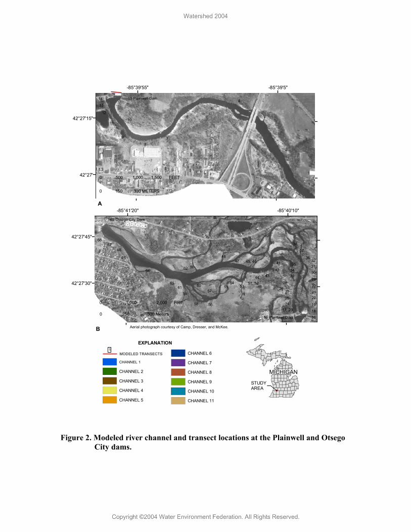
The study reach has four low-head dams. Three of these dams, Plainwell, Otsego, and Trowbridge, were decommissioned as power generators in the mid-1960s. The super-structures, consisting of powerhouses, gates, upper abutment walls, and some of the spillways, were removed in 1985-86 (Camp Dresser and McKee, 1999a). The current (2004) structures consist of only the dam foundations. The Otsego City dam super-structure is still intact but the dam is not functional. For modeling purposes, the entire study reach was divided into 15 channels, with a total of 131 transects. Channel 1 to channel 11 are between the Plainwell and Otsego City dams; channel 12 to 14 are between the Otsego City, Otsego, and Trowbridge dams. Channel 15, which is a short reach composed of 5 transects, is below the Trowbridge dam (Figures 2 and 3).

Kal

amaz

oo

River

R er

Kalamazoo

Dire

ction

of f

low

Direction of flow

49 iv

-85°39'55" -85°39'5"

14 15 Plainwell Dam 4 13

5 12

6 342°27'15" 10 11

9 7 8

2

42°27' 0 500 1,000 1,500 FEET 1

0 150 300 METERS

A -85°41'20" -85°40'10"

69 Otsego City Dam

42°27'45" 68

39 3867 66 37

48 40 3665 32 31

47 45, 46 41 35 62 50

42 3464 30 44 43 33

29 42°27'30" 63 54 51, 52 28

61 60 55 53 26 22

5957 27 21

25 20 0 1,000 2,000 Feet 58 56 24 19

17, 23 180 250 500 Meters

15 Plainwell Dam 16

B Aerial photograph courtesy of Camp, Dresser, and McKee.

EXPLANATION 1

MODELED TRANSECTS CHANNEL 6

CHANNEL 1 CHANNEL 7

CHANNEL 2 CHANNEL 8 MICHIGAN CHANNEL 3 CHANNEL 9 STUDY

AREA CHANNEL 4 CHANNEL 10

CHANNEL 5 CHANNEL 11

Figure 2. Modeled river channel and transect locations at the Plainwell and Otsego

City dams.

K a l a m z oo

Rve

r

K a l a m a o o R iver

81, 82 a

117 z

i

-85°44'30" -85°42'

97 Otsego Dam

42°28' 96 69 Otsego City Dam 95

93 78 7691 7079 7794 75 7392 90

89 80 74 72 71

88 84 83

87 8586

0 1,000 2,000 FEET

0 250 500 METERS 42°27'

A -85°47'0" -85°45'0"

114 126 Trowbridge Dam

124 122 120 113 42°29' 131 128 119 115

116 112 130 129 127 121 107

125 123 118 106

111

108 105 109

110 104

102 103

101 0 1,000 2,000 Feet

42°28' 99100 98

0 250 500 Meters 97 Otsego Dam

B Aerial photograph courtesy of Camp, Dresser, and McKee.

EXPLANATION

1 MODELED TRANSECTS

CHANNEL 12 MICHIGAN

CHANNEL 13 STUDY

CHANNEL 14 AREA

CHANNEL 15

Figure 3. Modeled river channel and transect locations at the Otsego and

Trowbridge dams.

METHODOLOGY

Sediment Transport Model Description

For this study, a mathematical sediment transport model “SEDMOD” was used that was developed by James P. Bennett (Bennett, 2001). It is a steady-state, 1-dimensional model, that simulates river flow and sediment transport in channel networks and computes the resultant scour and fill at any given location in the river reach. The model treats input hydrographs as step-wise steady-state, and the flow computation algorithm switches between sub- and supercritical flow as dictated by the channel geometry and discharge. Because the changes in channel geometry due to erosion and deposition occur relatively slowly as compared to the discharge hydrograph, the model approximates the hydrograph using a sequence of steady flows. The model allows the user to specify 20 sediment sizes, and any number of layers of known thickness. A brief description of the model structure and computational algorithms is given below.

Flow simulations

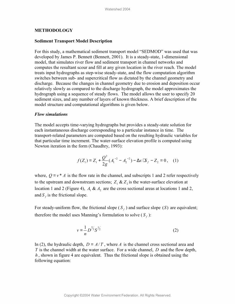
The model accepts time-varying hydrographs but provides a steady-state solution for each instantaneous discharge corresponding to a particular instance in time. The transport-related parameters are computed based on the resulting hydraulic variables for that particular time increment. The water-surface elevation profile is computed using Newton iteration in the form (Chaudhry, 1993):

f (Z1) = Z1 + Q2

( A1 −2 − A2

−2 ) − ∆x ⋅ S f − Z2 = 0 , (1)2g

where, Q = v * A is the flow rate in the channel, and subscripts 1 and 2 refer respectively to the upstream and downstream sections; Z1 & Z2 is the water-surface elevation at location 1 and 2 (Figure 4), A1 & A2 are the cross sectional areas at locations 1 and 2, and S f is the frictional slope.

For steady-uniform flow, the frictional slope ( S f ) and surface slope (S) are equivalent; therefore the model uses Manning’s formulation to solve ( S f ):

1 2 1 v = D 3 S 2 (2)

n

In (2), the hydraulic depth, D = A / T , where A is the channel cross sectional area and T is the channel width at the water surface. For a wide channel, D and the flow depth, h , shown in figure 4 are equivalent. Thus the frictional slope is obtained using the following equation:

S f = Q 2 ⋅ n1 ⋅ n2 ⋅ (T1 ⋅T2 )2

(3)(A1 ⋅ A2 )8

In the above equation, n is the Manning’s roughness coefficient, and T1 & T2 are the channel top widths at the upstream location 1 and downstream location 2. In figure 4, the upstream and downstream location has been given as 1 and 2, with h as the depth of flow and z as the reference bottom elevation. The other variable in figure 4 includes bottom shear stress (τ o ), velocity ( v ), and surface slope ( S ).

Figure 4. Definition of flow related variables (Bennett, 2001).

The upstream boundary condition in the model is always a specified discharge, with five user-specified boundary conditions for the downstream channel section. These include specified water-surface elevations time series, hydraulic depth versus discharge rating curve, normal flow depth for the downstream channel with specified slope, water surface elevation at a specified internal channel junction, or a sharp crested weir elevation and crest width.

The model allows network simulations, which may consist of several channels interconnected at junctions. The channel junctions are assumed to have no plan area, so no storage of water or sediment is recorded into it; also all channels entering or leaving the junctions have the same water-surface elevations. For each time step, the flow-simulation algorithm iterates through the entire network until neither the downstream water-surface elevation nor the input discharge varies significantly for any channel (Bennett, 2001). Water-surface elevation at a junction is determined by adjusting the sum of the discharges leaving the junction to that entering by less than a factor of 1 in 1000.

After all the flow rates have been determined in all the channels, sediment is distributed in the modeled system in proportion to the flow rates.

Bedload transport

The bedload transport equations for this model follow the work of Wiberg (1987) in incorporating Meyer-Peter-type formulation. The Wiberg model is based on the equations of motion for a sediment grain near a noncohesive bed, which include drag, lift, gravity, and relative concentration. A numerical solution of these equations will provide a path for the saltating particles, from which saltation height, length, and particle velocity can be computed. The model can be used to determine the thickness of the saltation layer and the amount of material transported therein (Bennett, 2001).

Wiberg (1987) concludes that a Meyer-Peter-type formulation works best to compute the bedload transport, assuming transport in equilibrium with bed-sediment of known size distribution f i (∑ fi = 1) for the i' th size fraction, which is shown in the equation below:

1.5φi = f iφ0 (τ * ′ − ( )τ * cr ) (4)

In (4), the non-dimensional bedload transport:

φi = bi [( )−1 gd i ] , (5)

3 0.5 s

where, bi is the unit volumetric bedload transport rate and di is the particle size for size fraction i , and s is the ratio of specific gravity of the bed material. Also in (4), the non-dimensional bottom shear stress:

τ ′ τ * ′ = O , (6) γ (s − 1)di

where, γ is the unit weight of water, and τ 0 ′ is the channel bottom shear stress (Figure 4) corrected for the form drag of any bed forms that are present. The critical shield stress τ * is based on d50 , the median bed-sediment size (50 percent of the bed particles are

cr

finer). That is, τ * cr results from (6), with d replaced by d50 andτ ′ by τ

cr , the sheari 0 *

stress for incipient motion for particles of the median bed-sediment size. The model uses a value of φo = 8, as adapted by Meyer-Peter and Muller (Bennett, 2001). This is a default value in the model and is user-adjustable.

Suspended-sediment transport

Computation of suspended load requires accurate representation of vertical variation of velocity and eddy diffusivity. The shape of the vertical profile of the longitudinal velocity

and the resistance to flow are determined from the size, shape, and spatial distribution of the roughness elements on the channel bed. The velocity profile for fully developed turbulent flow over a plane bed can be expressed as (Bennett, 1995):

ln

, (7)µ 1 z =µ* k zo

in which µ stream velocity at elevation z above the stream bed; κ = Von Karman’s constant with a value of 0.4; zo = the characteristic roughness height and it is the distance above the bed at which zero velocity occurs; and µ* = shear velocity. The eddy diffusivity for the velocity profile can be determined using the definition of eddy viscosity and Reynolds analogy. Using the definition of eddy diffusivity, and differentiating equation (7), the eddy diffusivity for a logarithmic velocity profile is obtained by the following equation:

ρ dµ

dz

τ κµ z(h − z)*ε (8)= = hs

In (8), τ = the boundary shear stress; and ρ = the density of fluid. Assuming steady, uniform flow and equilibrium transport in the longitudinal direction, the vertical conservation of mass equation for suspended-sediment for each size fraction can be solved analytically to yield:

vs

h − z 1

κµ* , (9)C = Cz a z h − a

where, Cz = the concentration at elevation z above the bed; vs = the fall velocity of the sediment; and a = the height above the bed at which the reference concentration is

vsspecified. Equation (9) is known as the Rouse equation and is the Rouse number. µ*

For computing reference-level concentration, the model uses the formulation from Smith and McLean (Bennett, 2001):

' Cbγ o S*Ca = , (10) 1 + γ S '* o

where, Cb = the volume concentration of sediment in the bed and is on the order of 0.65; γ o = a dimensionless parameter, with a default value of 0.004 and is user adjustable

'during simulations, and S * = the normalized excess shear stress or transport strength.

This type of formulation in the model is based on the assumption that equilibrium exists between the bed material make-up and the transport above it for a uniform reach.

Field Data Collection

Data for approximately 160 river cross sections were collected between the Plainwell and Trowbridge impoundments. Some of the low flow river reaches between the Plainwell and Otsego City dams were not included in the model due to stage-dependent flow directions, which require transient flow simulations that are beyond the scope of this study.

A total of 125 surveyed and 6 synthesized transects were used in the sediment-transport simulations. The synthesized transects were generated from surveyed adjacent channel geometries to provide additional geometry data to the model mainly at network junctions. The transect spacing was based on the average river width of each of the respective dams. Transect 1 in each impoundment was laid out as close to the dam as safety would allow. Transects 2, 3, and 4 were spaced at intervals of one river width. Transects 5, 6, and 7 were spaced at intervals of two river widths. Transects 8 and higher were spaced at four times the river width until the backwater end of each impoundment was reached. Increased river velocities, riffles, and debris islands typically indicated the backwater edge.

Reference points (RP) were established at each transect by driving a steel fence post into the bank, close to the water’s edge. Elevations of the RPs were surveyed to 0.1 ft by Camp Dresser and McKee in the fall of 2000. Elevations of bank height and water surface were calculated from the RPs at each transect.

A 3/16” steel-cable tagline, painted at 5-ft intervals, was stretched perpendicular to the river at each transect. Global Positioning System (GPS) coordinates were taken at both attachment points. The river width was divided into an average of 10 equal sections for the collection of depth of water, velocity, and sediment thickness. A GPS coordinate was taken at each section. Water depth and velocity were obtained by standard USGS meth-ods using a boat-cable measuring device equipped with an A-reel, 15 or 30 lb. weight, and a Price AA standard current meter.

Auger points samples and sediment cores were collected along each transect in the impoundments. Miscellaneous auger samples were taken between transects to improve contouring accuracy. Thickness of sediment was obtained by boring with a 1-ft long by 11/2-inch diameter auger bit with 4-ft extension pipes. The depth of the fill that overlaid the original river alluvium was indicated when the auger reached resistance and a grinding sound on cobble and stones could be heard. Sediment core samples were collected by driving a 10-foot length of 11/4-inch diameter PVC pipe into the river bottom until it reached resistance. Changes in texture and color were described and recorded in the field. Lithologic descriptions of the cores are summarized in Rheaume and others (2000). A total of 82 representative samples of these cores were collected and sieved using U.S. Standards Sieves between 0.0625 and 16 mm.

The suspended-sediment discharge was determined from suspended-sediment sample concentrations that were collected in accordance with the procedures described in Edwards & Glysson (1999). Bedload samples were collected with “US BL-84 Bedload Sampler”, developed by the U.S. Army Corps of Engineers, Waterways Experiment Station (http://fisp.wes.army.mil). These samples were collected near the Plainwell station (Station # 04106906) and downstream of the Trowbridge Dam, near the Allegan station (Station # 04107850). Data from the bed- and suspended-load samples collected at the Plainwell station were used as “input sediment supply rate” in the model simulations, and the data collected near the Allegan station was used to calibrate the model.

Model Input Data Structure

The network structure, channel geometry, and boundary condition data of the model reside in two flat files. The first, the network description file, describes the network interconnections, channel geometry, and sediment sizes and distribution. The second, the boundary condition file, sets the type and time span of simulation and describes all internal and external boundary conditions.

Network description file

In general, the network consists of a numbered sequence of channels for reference by the model algorithms; for example, there were a total of 15 channels or reaches in this study. The individual channels consist of a minimum of 2 and a maximum of 29 cross sections. A total of 131 cross sections with 11 junctions were modeled in the entire study reach, with cross section 1 the most upstream transect and cross section 131 the most downstream transect. The sediment-transport algorithm routes sediment in the sequence order in which channel descriptions are supplied.

The hydraulic component of “SEDMOD” is based on a stage-discharge boundary condition. The upstream boundary condition is the daily-mean flow rate at the most upstream river cross section and the downstream boundary condition is the daily-mean stage data at the most downstream cross section. The model uses a step-backwater approach to solve for the hydraulic variables in each reach. For each interior channel, discharge is a variable to be solved for and the boundary conditions at its ends are water-surface elevations at the respective junctions.

For the 730-day simulations (2001-2002 calendar year), daily mean discharge values from the Plainwell station (Station # 04106906) were used as the upstream boundary condition and stage data from Allegan station (Station # 04107850) was used as the downstream boundary condition. For the 1947 flood scenario, daily mean discharge data from the Comstock and Fennville station was used with necessary adjustments for drainage basin area. The Comstock station is upstream of the Plainwell station, and the Fennville station is downstream of Allegan station.

The model provides a plan-view plot of the simulation area. Therefore, the distance between cross sections is calculated using its coordinates to locate each transect’s base

line in the x-y plan view. A Universal Transverse Mercator (UTM) coordinate system was used in the model. Other necessary information for each cross section description includes an elevation adjustment factor (that may equal 0), a bedrock elevation or lower scour limit, and Manning’s n (based on site material) for the bedrock surface. The scour limit elevations were determined based on the elevation at which the sediment core reached resistance and a grinding sound on cobble and stones could be heard. A Manning’s n value of 0.04 was used for the bedrock material (Sturm, 2001). The Manning’s n value applicable to the full width of alluvial surface was computed for the individual cross section, based on the field data (See the section below for the computations of Manning’s n). The bank and (horizontal) bedrock segments comprise a no-erosion boundary for each cross section. A Manning’s n value of 0.05 was used for the right and left overbanks (Sturm, 2001), where information regarding vegetation cover and bank elevations could be derived from aerial photos.

Following description of the cross section geometry, the characteristics of different layers of sediment were entered into the network description file. Most of the cross sections in individual reaches had more than one sediment layer. They are numbered from the upper layer downward and, for each subsequent layer, the first record of the layer description includes a layer-surface elevation following the size-distribution code. Sediment size distributions were input into the model as fraction finer and the corresponding particle sizes. That is, listing fi as the volume percentage of the sediment layer that has sizes finer than the particle size di, thus, d50, is the particle size such that 50 percent of the layer-volume consists of finer particles. A total of eight sediment sizes between 0.0625 and 16 millimeters were used for individual sediment layers in the model simulations. The final section of the network description file describes the channel junctions from upstream to downstream.

Boundary condition file

The boundary condition file contains information to set the initial conditions for the model run, to determine the temporal extent of the simulation, and to specify appropriate boundary conditions for each time step during execution. In general, this file contains all the necessary information applied to the different boundary conditions, such as the upstream flow, the downstream stages, temperature in °C, and sediment supply rates. The temperature data are necessary to determine fall velocity and critical shear stress values for the particles of the simulation size classes. Temperature data were collected at the Allegan station and were used for the entire study section.

One of the data requirements for the model was to specify the total sediment transport rate that is coming into the study reach at the most upstream channel reach. Because the suspended sediment field data are reported as a concentration (mg/L) and the bedload data are reported as a loading rate (mass/unit time), proper conversion procedures had to be followed to convert them into a transport rate (m3/sec). After conversion, the bed- and suspended-load values had to be added to obtain the total transport rate for use by the model.

The final downstream boundary condition specifies the existence of a sharp-crested weir and requires the user to provide an absolute crest elevation and crest length, both in meters. This boundary condition was applied at an internal junction, providing the capability to include a low-head dam or diversion structure in the simulation. This boundary condition was applied to all four dams in the study reach.

Computations of Manning’s Roughness Coefficient

The average value of Manning’s roughness coefficient for each transect was computed using equation (11). This equation is applicable to a multi-section reach of M cross sections that are designated 1, 2, 3, ….M-1, M. Therefore, the entire Kalamazoo study reach was divided into several channel segments, each composed of a minimum of 2 and maximum of 4 transects. Input data into equation (11), such as discharge rate and water-surface elevations were used based on the field records during which they were collected for that specific transect. The hydraulic radius, cross sectional area, and wetted perimeter for each transect were computed from the field data using AutoCAD. After compiling all the input data, the final computations for Manning’s n were completed using MathCAD.

(h + hv)1 − (h + hv)m − [(k∆hv)1.2 + (k∆hv)2.3 + ... + (k∆hv)(M −1)M ] (11)1.486 n =

Q L1.2 + L2.3 + ....

L(M −1)M

Z1 Z 2 Z 2 Z 3 Z (M −1) Z (M )

In (11), n = Manning’s roughness coefficient; Q = discharge in cubic feet per second; h = elevation of water surface at the respective sections above a common datum; ∆hv = upstream velocity head minus the downstream velocity head; L = Distance between two cross sections; Z = AR2 / 3 ; A is the cross sectional area of the transect; R is the hydraulic radius, and k = a coefficient taken to be zero for contracting reaches and 0.5 for expanding reaches.

MODEL CALIBRATION

Calibration is the process of adjusting model parameters to obtain best fit of the model-computed results to the observed field data. The process can be completed manually using engineering judgment by repeatedly adjusting parameters, computing, and inspecting the goodness of fit between the computed and observed data. However, significant efficiencies can be achieved with an automated procedure.

The quantitative measure of the goodness-of-fit is the objective function. An objective function measures the degree of variation between the computed and observed values. It is equal to zero if the values are exactly identical. A minimum objective function is obtained when the parameter values are best able to reproduce the observed values. The adjustment should always be performed while keeping in mind that these parameters represent some physical process and therefore there should be a reasonable physical bound or constraint beyond which they should not be adjusted.

In this study, root mean square error (RMSE) was used as an objective function for measuring the goodness-of-fit between the model-computed and observed suspended-sediment transport rates. The field data used for calibration were collected near the Allegan station (transect 128), channel 15, during January 1, 2001 to December 31, 2001. In the model, the term γ o of equation (10) from McLean (Bennett, 2001) was used a calibration parameter. This coefficient sets the concentration at the base of the suspended transport layer and provides the only direct mechanism within the model to calibrate or adjust predicted suspended-sediment transport rates to match the observed rates. The McLean coefficient is a dimensionless parameter.

The McLean coefficient was adjusted manually for each model run, with a constraint limit set between 0.0013 and 0.008. The specified range for the McLean coefficient was chosen based on results obtained from model runs outside the chosen range. Model runs outside the specified range of McLean coefficient show oscillations and in some cases no convergence of the model solution. After each model run with a specified McLean coefficient, RMSE was computed using computed and observed suspended-sediment rates. The values of RMSE obtained along with specified values of the McLean coefficient for each model run are shown in figure 5. The minimum value of objective function (RMSE) achieved was 0.0028 using a McLean coefficient of 0.004. The residuals obtained from the minimized objective function value are shown in figure 6. Analysis of the residual plot and discharge hydrograph show a slight bias in the model results under high-flow conditions (flows higher than 80 m3/sec), which means that the model-computed suspended-sediment transport rates are higher compared to the observed data. However, the overall calibrated model results show close agreement between simulated and measured values of suspended sediments.

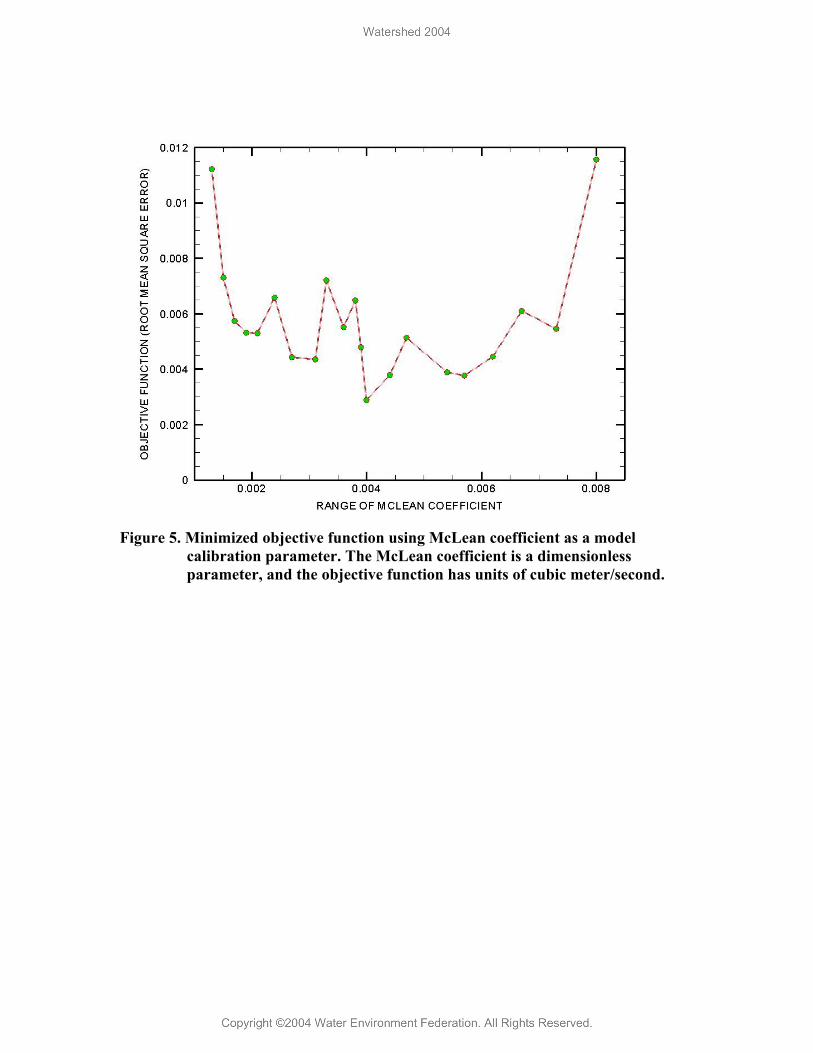
Figure 5. Minimized objective function using McLean coefficient as a model calibration parameter. The McLean coefficient is a dimensionless parameter, and the objective function has units of cubic meter/second.

Figure 6. Calibrated model residuals, achieved with a McLean coefficient value of 0.004. Suspended-sediment units are in cubic meter/second.

SEDIMENT-TRANSPORT MODEL RESULTS

The model results are based on the following three scenarios: 1) Sediment-transport simulations for 730 days (Jan. 2001 to Dec. 2002), with

existing dam structures; 2) Sediment-transport simulations using flows from the 1947 flood at the Kalamazoo

River with “existing dam structures;” and 3) Sediment transport simulations using flows from the 1947 flood at the Kalamazoo

River with “no dam structures.”

Sediment Transport Simulations for 730 days (Jan. 2001 to Dec. 2002), with Existing Dam Structures

For this scenario, the sediment transport model runs for a total time period of 730 days (January 1, 2001 to December 31, 2002). The results obtained were analyzed in three categories: 1) Total volume and size distribution of in-stream sediments, (conditions before simulations); and 2) sediment erosion and deposition rates and volumes during the simulation period; 3) significant changes observed in sediment-bed elevations and d50 during the simulation period (Jan. 2001 to Dec. 2002).

Total volume and size distribution of in-stream sediments

The model computes the total volume of sediments in any channel segment between cross sections of interest, based on the transect geometry and core sample data. In this report, details regarding the volume of in-stream sediments in the study reach have been limited only to the backwater reach of each impoundment. This is because most of the in-stream sediments in the study area are present behind the dams, and significant bed-elevation changes due to variable flow conditions are noticeable mainly in these sections. The total volume of sediments in the backwater section of each impoundment has been described in Table 1.

Table 1. Volume of in-stream sediments in the backwater section of each dam.

Sediment erosion and deposition rates and volumes during the simulation period

In this section of the report, sediment transport results are presented based on the magnitude of flow rates that triggered changes in sediment erosion or deposition rates during the simulation period. Analysis of the model results shows that significant sediment erosion from the study reach occurred at flow rates higher than 55 m3/sec. Sediment deposition mainly occurred during low-to-average flow conditions (monthly mean flows between 25.49 m3/sec and 50.97 m3/sec), following a high flow event until the system reached equilibrium.

During the 730-day simulation, high flow events occurred from February 9 to March 8, 2001 (maximum discharge rate 117m3/sec.); May 14 to June 8, 2001 (maximum discharge rate 104 m3/sec); October 14 to November 4, 2001 (maximum discharge rate 68 m3/sec); and March 3 to March 18, 2002 (maximum discharge rate 81 m3/sec). During these four flow events, model results show a total sediment erosion of approximately 88,890; 7,400; 3,600; and 3,600 cubic meters respectively from the study reach. Transport rates and associated volume errors are shown in Table 2.

Sediment deposition mainly occurred during low-to-average flow conditions (monthly mean flows between 25.49 m3/sec and 50.97 m3/sec) following a high-flow event. For example, deposition was dominant in the study reach for a short time period after a high-flow event in March 2001. During this time period, the average sediment-supply rate into the study reach was approximately 71 metric tons/day, and the total sediment loss from the system was approximately 57 metric tons/day. Similarly, the average sediment-deposition rates are in the range of 4 to 15 metric tons/day after the June and November 2001 and March 2002 high flow events.

The total amount of sediment eroded at the end of 2001 was approximately 164,000 m3. The total amount of sediment eroded at the end of year 2002 was approximately 12,200 m3. Higher erosion rates for the first year are due to the high magnitude of discharge rates that occurred compared to 2002. An assessment of the study reach at the end of 730 days shows that degradation is significant in channels 1, 8, and 9 (Figure 2 and 3). From these channels, a total volume of approximately 45,410 m3, 37,650 m3, and 57,230 m3, respectively of in-stream sediments was eroded during the 730-day simulation period.

Significant levels of sediment deposition occurred in channels 13, 14, and 15, which are the most downstream channels in the study section (Figure 2 and 3). In channels 13, 14 and 15, a total volume of approximately 31,000 m3, 21,000 m3, and 17,000 m3, respectively, of sediments is deposited during a time period of 730 days (Jan. 2001-Dec. 2002). Total sediment-transport rates during the simulation period 2001-2002 are shown in figure 7.

Table 2. Model-computed sediment transport rates during the high-flow events (January 2001 to December 2002).

Figure 7. Model-computed total sediment transport rates during the simulation period January 2001 to December 2002.

Significant changes observed in sediment-bed elevations and d50s during the simulation period (Jan. 2001 to Dec. 2002)

The model keeps track of the bed-elevation changes and sediment-size composition (d50) during simulation at each cross section. Model results show that there were significant changes in bed elevations during high flows such as during February 9 to March 8, 2001 (maximum discharge rate 117m3/sec.); May 14 to June 8, 2001 (maximum discharge rate 104 m3/sec); October 14 to November 4, 2001 (maximum discharge rate 68 m3/sec); and March 3 to March 18, 2002 (maximum discharge rate 81 m3/sec). Based on the model results, scour or degradation mainly occurred in channel segments upstream of the Plainwell, and Otsego City dams. Deposition occurred in channel 13, 14, and 15 (Figure 2 and 3).

Cross sections that showed significant changes in bed elevation during the simulation period include:

• In channel 1, cross section 13, which is located close to the Plainwell dam, bed scour occurred in the range of 0.6 meters (1.97 ft), during the February 9 to March 8, 2001, high flows. Under average or normal flows, the bed started building up again. This can be observed during low-to-average flow conditions (Figure 8).

• In channel 11, cross section 50, which is located at the confluence of channel 9, 10, and 11, where channel 9 and 10 forms a junction and flows into channel 11 (Figure 2), degradation of approximately 0.8 meters (2.64 ft) occurs during the high flows of February 9 to March 8, 2001 (Figure 9). The bed elevation stays the same for the rest of the simulation period.

• In channel 11, cross section 64 changes in bed elevation respond to the changes flow rates. Bed scour occurs in the range of 0.4 meters (1.31 ft) during high flow conditions. Under average or normal flows the bed start building up again. This can be observed during low-to-average flow conditions (Figure 10).

• Cross section 93 in channel 13 show defined changes in sediment-bed elevations and d50 in response to the changing flow conditions (Figure 11).

The bed elevation field data collected during the transect surveys was used as an input into the model. No further bed elevation data was collected to validate the model-computed elevations at the end of the study period.

Figure 8. Cross section 13, changes observed in bed elevations and sediment d50 during the 730-day model simulations.

Figure 9. Cross section 50, changes observed in bed elevations and sediment d50 during the 730-day model simulations.

Figure 10. Cross section 64, changes observed in bed elevations and sediment d50 during the 730-day model simulations.

Figure 11. Cross section 93, changes observed in bed elevations and sediment d50 during the 730-day model simulations.

Sediment Transport Simulation Results, Using Flows From the 1947 Flood at the Kalamazoo River with “Existing Dam Structures” and “Dams Removed”.

The highest discharge recorded in the Kalamazoo River system occurred during the 1947 flood (peak flow 235.2 m3/sec). Sediment-transport simulations using the 1947 flood hydrograph provide an estimate of sediment-transport rates under maximum flow conditions. This scenario also provides an assessment of the sediment load that may erode from the study section during a catastrophic dam failure.

For the 1947 flood scenario, the model uses the same “network description file” as that used for the January 2001 to December 2002, model simulation. The fixed boundary conditions such as the transect geometry, bed elevations, and sediment-size distribution are the same in all model scenarios. The flows and stages used in the “1947 flood scenario” have been derived from the Comstock and Fennville stations. The sediment-supply rates into the study section have been estimated based on the field data collected near the Plainwell station under high-flow conditions. During simulations, the model routes the 1947 flood hydrograph through the study section using two different conditions: 1) 1947 flood with existing or current dam structures in the study section; 2) and 1947 flood with no dam structures in the study

section. The main difference between the “dam in” and “dam out” scenarios is that the former considers all the current dam structures present in the study section during the simulation period but the latter assumes that none of the dam structures exist in the study section during the simulation period.

The model runs for a total time period of sixty days, with a peak discharge of 235.2 m3/sec. The flood hydrograph starts rising at day 10, with a peak flow at day 15, and then recedes at day 21. It starts rising again at day 31 (peak flow of 83.10 m3/sec.) and day 43 (peak flow of 77.20 m3/sec.) (Figure 12).

Analyses of the model results for the first 21 days with the “dam in” scenario show a total in-stream sediment loss or erosion of approximately 127,600 m3 from the entire study reach, with a total volume error of 100 m3. The peak transport rate ranges from .00165 m3/sec (377 metric tons/day) to 0.16800 m3/sec (38465 metric tons/day).

Similarly, for the first 21 days during the “dam out” scenario a total in-stream sediment loss or erosion of approximately 152,700 m3 from the entire study reach occurs with a total volume error of 171 m3. There is 25,000 m3 more loss of in-stream sediments as compared to the “1947 flood with dam in” scenario. The peak transport rate during this time is in the range of .00064 m3/sec (146 metric tons/day) to 0.17660 m3/sec (40434 metric tons/day) (Table 3).

Table 3. Model computed sediment transport rates during the 1947 flood simulations “with dams”.

For the “dam in” scenario, the model results show that degradation is significant in channels 1, 8, and 9, with a total degradation of approximately 42,190 m3, 26,450 m3, and 62,870 m3, respectively during the 60-day time period. Aggradation or deposition occurred in channels 12, 13, 14, and 15 with total volumes of approximately 3,893m3, 17,490m3, 1,503m3, and 5,773 m3, respectively. Channels 12 and 13 are between the Otsego City and Otsego dams; channel 14 is between the Otsego and Trowbridge dams; and channel 15 is downstream of the Trowbridge dam.

For the “dam out” scenario, model results show that degradation is significant in channel, 1, 8 and 9, with a total degradation of approximately 43,490 m3, 26,190 m3 and 72,320

m3, respectively during the 60-day time period. Aggradations occurred in channels 12, 13 and 15 with volumes of approximately 22,010 m3, 19,300 m3, and 8,967 m3, respectively. Comparison of the total sediment-transport rates for the “dam in” and “dam out” scenarios that occurred during the 60-day period is shown in figure 12 and 13.

Figure 12. Model-computed total sediment-transport rates during simulation of 1947 flood event with current (2004) dam conditions.

Figure 13. Model-computed total sediment-transport rate during simulation of 1947 flood event with catastrophic dam failure.

DISCUSSION & CONCLUSIONS

Analyses of the model results show that the Kalamazoo River sediment-transport mechanism is in a dynamic equilibrium state. Sediment loss, or erosion, from the study reach mainly occurs during high flows (flows larger than 55 m3/sec.), followed by a short depositional period during low-to-average flows (monthly mean flows between 25.49 m3/sec and 50.97 m3/sec) until the system reaches equilibrium.

During the 730-day model simulations, high-flow events occur from February 9 to March 8, 2001 (maximum discharge rate 117 m3/sec.); May 14 to June 8, 2001 (maximum discharge rate 104 m3/sec); October 14 to November 4, 2001 (maximum discharge rate 68 m3/sec); and March 3 to March 18, 2002 (maximum discharge rate 81 m3/sec). During these four flow events, model results show a total sediment erosion of approximately 88,890; 7,400; 3,600; and 3,600 cubic meters respectively from the study reach.

Sediment deposition mainly occurs during low-to-average flow conditions (monthly mean flows between 25.49 m3/sec and 50.97 m3/sec), following a high-flow event. For example, deposition occurs for a short time period after the high-flow event in March 2001. During this time period, the average sediment-supply rate into the study reach is

approximately 71 metric tons/day and the total sediment loss from the system is approximately 57 metric tons/day. Similarly, the average sediment-deposition rates are in the range of 4 to 15 metric tons/day after the June and November 2001, and March 2002 high-flow events. If the flows continue to stay in the low-to-average state, then the system shifts towards equilibrium. This results in a balancing effect between sediment deposition and erosion rates.

There are no significant differences between the transport rates during the “dam in” and the “dam out” scenarios under the 1947 flood flow conditions. There is approximately 25,000 cubic meters more erosion of in-stream sediments during the “dams out” scenario compared to the “dams in” simulations, with the same initial conditions during both scenarios. This occurs because the dams in the study reach have low heads and no control gates. Therefore, during high-flow conditions approximately the same magnitudes of velocities are generated in the backwater sections during both scenarios, which produces the same impact on sediment erosion rates. It is important to note that the “dam in” and “dam out” scenarios simulations are run for only 60 days, which takes into account only the instantaneous changes in sediment erosion and deposition rates during that time period. Over an extended period of time, it is expected that more erosion will occur if the dams are removed from the study reach compared to the existing conditions. Removal of dams would further lower the head in all the channels, producing higher velocities even during low-to-average flow conditions, which would result in accelerated erosion rates throughout the study reach.

The Kalamazoo River network, particularly the braided portion between the Plainwell and Otsego City dams, offers a great deal of complexity to simulate in any hydraulic model. The direction of flow in some of the braided channels is discharge-dependent, which means that reverse flow conditions can occur under certain discharge rates. Although SEDMOD is capable of computing flow and sediment transport through multiple networks, it cannot take into account reverse flow conditions. Therefore, only those braided channels between the Plainwell and Otsego City dams have been modeled where the flow is in one direction and enough slope is present in the channel bottom such that reversed flow conditions would not occur. Elimination of some reaches from the model could produce high erosion rates due to excessive shear stress produced in the modeled channels during high flow conditions compared to the flow distribution in the natural system. This could impact sediment deposition and erosion estimates produced by the model.

It is important to note that the “dam failure or removal” in the modeling scenarios does not mean a “dam breach.” Instead it represents the removal of a non-erodible structure such as a sharp crested weir with a defined geometry. Therefore, the model results generated under the “dam removal” scenario show the changes in the hydraulics of the flow and the associated sediment-transport processes resulting from the removal of the non erodible structure rather than an actual dam failure event.

ACKNOWLEDGMENTS

This study was conducted by the USGS in cooperation with Shari Kolak, Remedial Project Manager, Region 5, Superfund Divison (U.S. EPA); and Paul Bucholtz, Environmental Quality Analyst (MDEQ). The authors express their appreciation to the many people who provided help and participated in the collection and analysis of data and in the preparation and review of this paper. Todd King, of the Camp, Dresser, and McKee, Inc. provided technical support. Stephen Rheaume, Richard Hubbel, and Cynthia Rachol participated in the field data collection and provided a quality data set from which the model input files were built. Andreanne Simard performed all the sieve analysis for the transect core samples. Denis Healy provided valuable information regarding model input files and developed the network description file for the lower two dams. David Holtschlag provided valuable advice regarding the flow distribution in the braided portion of the Kalamazoo River. Lori Fuller provided GIS support.

REFERENCES

Bennett J. P. (1995) Algorithm for Resistance to Flow and Transport in Sand-Bed-Channels: Journal of Hydraulic Engineering, 121 (8), 578.

Bennett J. P. (2001) User’s Guide for Mixed-Sized Sediment Transport Model for Networks of One-Dimensional Open Channels; Water Resources Investigations Report 01-4054; U.S. Geological Survey.

Blumer, S.P.; Behrendt, T.E.; Ellis, J.M.; Minnerick, R.J.; LeuVoy, R.L.; Whited, C.R. (2000) Water resources data, Michigan, water year 2000; Water-Data Report MI-00-1; U.S. Geological Survey.

Chaudhry, M.H. (1993) Open Channel Flow, Englewood Cliffs, N.J., Prentice Hall.

Edwards. T. K.; Glysson, D.G. (1999) Field Methods for Measurement of Fluvial Sediments; Water Resources Investigations Report, Book 3; U.S. Geological Survey.

Federal Interagency Sedimentation Project, Sampling with the US BL-84 Bedload Sampler, http://fisp.wes.army.mil

FEMA (Federal Emergency Management Agency), 1999, National Dam Safety Program, http://www.fema.gov/mit/ndspweb.htm.

Haan, C. T.; Barfield, B. J.; and Hayes, J. C. (1994) Design Hydrology and Sedimentology for Small Catchments; Academic Press, A Division of Harcourt Brace & Company.

Rheaume, S. J.; Rachol, C. M.; Hubbell, D. L.; and Andreanne Simard (2000) Sediment Characteristics and Configuration within Three Dam Impoundments on the

Kalamazoo River, Michigan; Water Resources Investigation Report 02-4098;U. S. Geological Survey.

Sturm, T.W. (2001) Open Channel Hydraulics; McGraw-Hill Series in Water Resources and Environmental Engineering, Ist Edition.

Wiberg, P.L. (1987) Mechanics of Bedload Sediment Transport; A dissertation submitted in partial fulfillment of the requirements for the degree of Doctor of Philosophy, University of Washington.