Analysis of natech risk for pipelines: A review

Roberta Piccinelli, Elisabeth Krausmann

2 0 1 3

Report EUR 26371 EN

European Commission Joint Research Centre Institute for the Protection and Security of the Citizen Contact information Elisabeth Krausmann Address: Joint Research Centre, Via Enrico Fermi 2749, TP 720, 21027 Ispra (VA), Italy E-mail: elisabeth.krausmann@jrc.ec.europa.eu http://ipsc.jrc.ec.europa.eu/ http://www.jrc.ec.europa.eu/ Cover photo: Trans-Alaska Pipeline System (http://dnr.alaska.gov/commis/priorities/securealaskasfuture_oil.html) Legal Notice Neither the European Commission nor any person acting on behalf of the Commission is responsible for the use which might be made of this publication. Europe Direct is a service to help you find answers to your questions about the European Union Freephone number (*): 00 800 6 7 8 9 10 11 (*) Certain mobile telephone operators do not allow access to 00 800 numbers or these calls may be billed.

A great deal of additional information on the European Union is available on the Internet. It can be accessed through the Europa server http://europa.eu/. JRC86630 EUR 26371 EN ISBN 978-92-79-34813-6 ISSN 1831-9424 doi:10.2788/42532 Luxembourg: Publications Office of the European Union, 2013 © European Union, 2013 Reproduction is authorised provided the source is acknowledged.

 

 

 

Analysis of natech risk for pipelines: 

A review  

Roberta Piccinelli and Elisabeth Krausmann

 

Abstract 

Natural  events,  such  as  earthquakes  and  floods,  can  trigger  accidents  in  oil  and  gas  pipeline  with potentially  severe  consequences  to  the  population  and  to  the  environment.  These  conjoint technological and natural disasters are termed natech accidents.  

The present  literature  review  focuses on  the  risk analysis  state‐of‐the‐art of  seismic and  flood events that can impact oil and gas transmission pipelines. The research has focused on methodologies that take into  account  the  characteristics  of  natech  events:  for  instance,  the  characterization  of  the  triggering natural hazard and the final accident scenarios, as well as fragility curves for the specific assessment of the potential consequences of natech accidents.  

The result of this research shows that the literature on seismic risk analysis offers the largest number of examples  and methodologies,  although most  studies  focused  on  structural  damage  aspects without considering the consequences of a potential loss of containment from the pipelines. Very little work was found on flood risk assessment of natech events in pipelines. 

 

 

Table of Contents 

 

1. Introduction .......................................................................................................................................... 1

2. Seismic vulnerability of pipelines .......................................................................................................... 3

2.1 Earthquake severity measures............................................................................................................ 3

2.2 Description of pipelines ...................................................................................................................... 6

2.3 Methodologies for seismic pipeline risk analysis................................................................................ 8

2.3.1 Pipeline damage due to earthquakes ........................................................................................10

2.3.2 Fragility estimation ....................................................................................................................12

2.3.2.1 State‐of‐the‐art of fragility curves for pipelines .....................................................................13

2.3.2.2 Studies including natech‐related aspects ...............................................................................24

3. Vulnerability of pipelines to floods .........................................................................................................28

3.1 Flood severity measures ...................................................................................................................29

3.2 Methodologies for pipeline risk analysis with respect to floods ......................................................29

3.2.1 Pipeline damage due to floods ..................................................................................................30

3.2.2 Fragility estimation ....................................................................................................................31

4. Conclusions .............................................................................................................................................35

References ..................................................................................................................................................37

 

1. Introduction 

Risk analysis asks the questions:  “What can go wrong? How likely is it to happen? What are the consequences?”  

A first observation comes from the fact that there is risk if there is a potential source of danger, so the answer  to  the  first  question  helps  to  identify  the  hazard  or  the  potential  adverse  events  and mechanisms by which  the events may create undesired consequences,  loss or damage. However,  the presence of a hazard is not sufficient to define a condition of risk. Indeed, it is necessary to consider the uncertainty that the hazard translates from potential to actual damage: the likelihood of damage related to the hazard is expressed through probabilities (Kaplan and Garrick, 1981). 

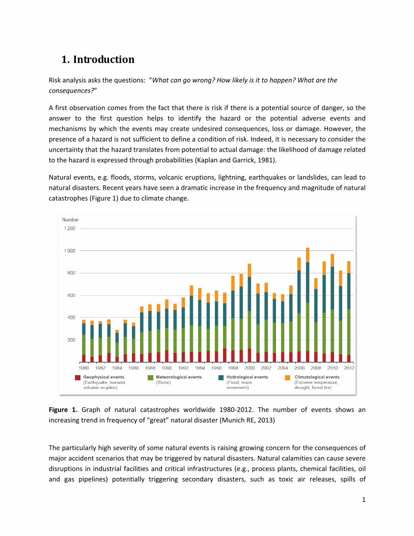
Natural events, e.g. floods, storms, volcanic eruptions,  lightning, earthquakes or  landslides, can  lead to natural disasters. Recent years have seen a dramatic increase in the frequency and magnitude of natural catastrophes (Figure 1) due to climate change.   

 

Figure  1.  Graph  of  natural  catastrophes  worldwide  1980‐2012.  The  number  of  events  shows  an increasing trend in frequency of “great” natural disaster (Munich RE, 2013)  

The particularly high severity of some natural events is raising growing concern for the consequences of major accident scenarios that may be triggered by natural disasters. Natural calamities can cause severe disruptions  in  industrial facilities and critical  infrastructures  (e.g., process plants, chemical facilities, oil and  gas  pipelines)  potentially  triggering  secondary  disasters,  such  as  toxic  air  releases,  spills  of 

  1

hazardous materials,  fires or explosions  (Young et al., 2004; Girgin, 2011; Krausmann et al, 2011 a,b). These conjoint natural and technological disasters are termed natech accidents. 

Natural  disasters  and  technological  accidents  have  generally  been  studied  as  separate  events; consequently,  little  information  on  their  interaction  was  produced.  Nevertheless,  there  is  growing awareness of the risk posed by the simultaneous  interaction of natural and technological hazards, and the  need  for  developing  integrated  methodologies  capable  of  estimating  damage  when  different typologies of hazard are present (Krausmann et al., 2011b).  

Studies of the natech accidents recorded  in the major  industrial–accident databases was performed to identify  the most  frequent natural disasters,  the most  vulnerable  equipment  categories,  their  failure mode and  the  resulting accident  scenarios  (Cozzani et al., 2010; Renni et al., 2010; Krausmann et al., 2011 a). Based on the operating conditions and the severity of potential accidental events associated, these  studies  called  attention  to  pipeline  natech  accidents  triggered  by  earthquakes  and  floods. Numerous  severe  accidents  bear  testimony  to  the  risk  associated  with  natural  hazard  impact  on pipelines transporting dangerous substances. In the USA in 1994, flooding of the San Jacinto River led to the rupture of 8 and the undermining of 29 pipelines by the flood waters. Subsequently, 5.5 million litres of petroleum and related products were released  into  the river and  ignited. Overall, 547 people were injured due to inhalation and burns (NTSB, 1996). 

Although pipeline  releases have caused  relatively  few  fatalities  in absolute numbers, a  single pipeline accident could be catastrophic in terms of deaths and environmental damage. The possibly wide spatial extent of natural disasters  such as earthquakes and  floods may actually  simultaneously affect  several equipment items of distributed systems such pipelines. Moreover, emergency response may be delayed by the natural event. 

Such accidents have generated persistent  scrutiny of pipeline  regulators and have  increased national and  community  activity  related  to  pipeline  safety  (Parfomak,  2013). Methodologies  and  tools,  e.g. RAPID‐N  (2013),  RAI2  (2012)  or  ARIPAR  (Campedel  et  al.,  2008),  for  the  specific  assessment  of  the potential  consequences  of  natech  accidents  are  only  recently  under  development  but  some  specific scenarios and models that  link the severity of the natural hazard to  its  impact on specific components are still missing (Krausmann et al., 2011 a).  

When  developing  a  specific  natech  approach  for  risk  assessment,  the  standard  risk  management procedure that should be adhered to is summarized in Table I. 

In  this  general  framework,  both  the  qualitative  and  the  quantitative  risk  analysis  need  to  take  into account the characteristics of natech events: for instance, a dedicated approach to the characterization of the triggering natural hazard or disaster and the final accident scenarios. 

From this (natech) standpoint, the present literature review focuses on the risk analysis state‐of‐the‐art of seismic and flood events that can impact (oil and gas) transmission pipelines. 

 

  2

Table I. Technical steps in the risk management process (Mannan, 2005; CCPS, 2000) 

Step  Activity 

1  Planning the risk management process: this involves the definition of the level of detail and the tools to use in the analysis 

2  Hazard  identification: this comprises all the activities required to  identify all hazards related to the examined system 

3  Qualitative risk analysis: this  involves screening activities aimed at  identifying where and when more detailed analyses are required 

4  Quantitative risk analysis: this involves quantifying both occurrence of probability and expected consequence magnitude of each identified hazard to estimate an overall risk index 

5  Planning  the mitigation measures:  this  requires  the  implementation of all  the prevention and protection measures necessary to keep the risk level below the acceptable threshold  

6  Risk monitoring and control: this comprises the activities required to avoid changes that would increase the risk level above the acceptable threshold 

2. Seismic vulnerability of pipelines 

The earthquake  impact on pipelines may  result  in  releases of hazardous materials and possibly major accidents leading to injuries and fatalities to people in the nearby area. In 1994, an oil spill of more than 3500 barrels occurred on  the Santa Clara River as a result of a pipeline rupture during  the Northridge (Colorado, USA) earthquake. Several  releases occurred  from  this break which caused approximately 5 miles of pipeline to empty to the ground and into the river (Leville et al., 1995). 

Most major  oil  and  gas  pipelines  generally  run  underground:  although  they  are  less  exposed  to  the inertial forces than the above‐ground pipelines, the seismic response of pipelines  is dominated by soil deformation, so that vulnerability assessment strongly depends on the ground – pipeline interaction. 

In  the  following,  a  literature  review of  earthquake  severity measures will be provided  together with fragility  curves,  which  give  the  probability  of  damage  based  on  specific  intensity  parameters,  or threshold  values of  the  seismic  intensity.  Fragility  curves  are  an essential  component of pipeline  risk analysis. 

2.1 Earthquake severity measures

A  main  issue  related  to  the  seismic  risk  analysis  of  pipelines  is  the  selection  of  an  appropriate earthquake intensity measure (IM) that characterizes the strong ground motion and best correlates with 

  3

the  response  of  each  element.  Several  measures  of  the  strength  of  ground  motion  have  been developed. Each intensity measure may describe different characteristics of the motion, some of which may be more damaging for the structure or system under consideration. The use of a particular  IM  in seismic  risk analysis should be guided by  the extent  to which  the measure corresponds  to damage  to local elements of a system or the global system itself. Optimum intensity measures are defined in terms of practicality, effectiveness, efficiency,  sufficiency,  robustness and computability  (Cornell et al, 2002; Mackie and Stojadinovich, 2003; 2005).  

• Practicality refers to the recognition that the IM has some direct correlation to known engineering quantities and that it “makes engineering sense” (Mackie and Stojadinivich, 2005; Mehanny, 2009).  

• Sufficiency  describes  the  extent  to  which  the  IM  is  statistically  independent  of  ground motion characteristics  such  as magnitude  and distance  (Padgett  et  al., 2008). A  sufficient  IM  is one  that renders the structural demand measure conditionally independent of the earthquake scenario.  

• The effectiveness of an  IM  is determined by  its ability to evaluate  its relation with an engineering demand parameter (EDP) in closed form (Mackie and Stojadinovich, 2003), so that the mean annual frequency  of  a  given  decision  variable  exceeding  a  given  limiting  value  (Mehanny,  2009)  can  be determined analytically.  

• The most widely used quantitative measure from which an optimal IM can be obtained is efficiency. This refers to the total variability of an engineering demand parameter for a given IM (Mackie and Stojadinovich, 2003; 2005).  

• Robustness  describes  the  efficiency  trends  of  an  IM‐EDP  pair  across  different  structures,  and therefore different fundamental period ranges (Mackie and Stojadinovich, 2005; Mehenny, 2009).  

In general, two main IM classes exist: empirical intensity measures and instrumental intensity measures. With regard to the empirical IMs, different macro‐seismic intensity scales could be used to identify the observed effects of ground shaking over a limited area. With respect to instrumental IMs, the severity of ground  shaking  can  be  expressed  as  an  analytical  value measured  by  an  instrument  or  computed through the analysis of recorded accelerograms.  

The  seismic  response of underground  structures  is  considerably different  from  that of  above‐ground facilities. While the latter ones act as a kind of inertial filter on the incident ground motion, the seismic response  of  buried  structures  is  dominated  by  the  surrounding  soil  deformation,  and  inertial  soil‐structure  interaction effects are generally negligible (St. John and Zahrah, 1987). Therefore, one of the critical  aspects  behind  the  seismic  design  and  assessment  of  underground  structures  is  the  proper definition of the input ground motion. The strain evaluation is important for the vulnerability, as well. A direct measure of  the ground strain  is not generally available, since strain networks are not generally equipped with strain‐meters; therefore, simplified formulas relating peak ground strain to peak ground velocity are typically used. 

  4

The  selection  of  the  intensity  parameter  is  also  related  to  the  approach  that  is  followed  for  the derivation of fragility curves and the type of element at risk. For example, as the empirical curves relate the observed damage with the seismic  intensity, the  latter may be described based on the  intensity of records of seismic motions, and thus peak ground acceleration (PGA) or peak ground velocity (PGV) may be  suitable  IMs. On  the  other  hand,  the  spatial  distribution  of  PGA  values  is  easier  to  be  estimated through simple or advanced methods within a seismic hazard study of a specific area (e.g., Esposito and Iervolino, 2011). When the vulnerability of elements due to ground failure is examined (i.e. liquefaction, fault  rupture,  landslides), permanent  ground deformation  (PGD)  is  the most  appropriate  IM.  Seismic fragility  curves  relate  pipeline  damage  rates  to  different  levels of  seismic  intensity.  In  the  literature, various  ground  motion  parameters  have  been  used  to  describe  the  seismic  event.  Here  a  brief description is presented. 

Previously,  seismic  intensity has been measured by using  the Modified Mercalli  Intensity Scale  (MMI) which is an empirical intensity measure. This scale is composed of 12 increasing levels of intensity that range from imperceptible shaking to catastrophic destruction: the lower numbers of the intensity scale generally deal with  the manner  in which  the earthquake  is  felt by people;  the higher numbers of  the scale are based on observed structural damage. This scale does not have a mathematical basis; instead it is an arbitrary ranking based on observed effects. The obtained values depend on the characteristics of the existing  structural  system and natural environment  (USGS, 2013). This  is a  limitation because  the description  is  restricted  to  local  characteristics and because  it  is not an objective  scale. Nevertheless MMI maps are still used and many relations for the performances of structures during earthquakes are dependent on MMI.  For example  Santella et  al.  (2011)  report  a delineation of  five  seismic  zones  for earthquakes using the MMI zones based on Shakemaps, obtained from the US Geological Survey (USGS) Earthquake Center (USGS, 2013).  

More  recently,  the  improvement  in measurement  techniques has  allowed  the use of more objective seismic parameters (instrumental intensity measures). The most significant synthetic parameters are the PGA and PGV. PGA is the peak of the horizontal acceleration time history. Since PGA is directly related to the  structure,  because  of  its  proportionality with  inertial  effects  due  to  seismic  loading,  it  is more appropriate  for  above‐ground  structures  (Lanzano  et  al.,  2013a).  For  underground  structures,  the damaging effects due to the passage of the seismic waves  in the soil are proportional to PGV, which  is the peak value of the horizontal velocity time histories.  

These parameters are only a concise description of the information of the local motion of the soil: they are available only at the instrumented site. Predictive correlations (attenuation laws) are used to give a value of the parameters for an extended area (Douglas, 2004). 

Based  on  the  experience  and  data  collected  during  past  earthquakes,  geotechnical  dynamics  effects related to pipeline damage can be divided in two categories (O’Rourke and Liu, 1999): 

• Strong Ground shaking  (SGS): the common effect  is a deformation of the soil which surrounds the pipeline, without breaks or ruptures in the soil, depending on the earthquake intensity; 

  5

• Ground  Failure  (GF):  the  surrounding  soil  is  affected  by  failure  phenomena  caused  by  the earthquake as active  fault movement  (GF1),  liquefaction  (GF2), and  landslides  induced by  the shaking  (GF3).  These  seismic  failure  mechanisms  appear  only  under  specific  geotechnical conditions and are site dependent.

2.2 Description of pipelines

Pipelines are important structural components in industrial and civil facilities. They are used to transport and  distribute  liquid  and  gaseous materials  such  as  oil  and  natural  gas  in  energy  assets,  hazardous chemicals and gases such as ammonia and ethylene  in process plants and water  in urban areas. Most hazardous  liquid and gas pipelines are buried underground, but there are several major above‐ground structures, such as the Trans‐Alaska Pipeline System. 

Based on their function, pipelines can be classified as (Hopkins, 2002): 

• Flow‐lines  and  gathering  lines:  these  short  distance  lines  gather  various  products  and move them towards processing facilities. 

• Feeder  lines: these pipelines move oil and gas  fluids  from processing  facilities, storage etc., to transmission lines. 

• Transmission lines: these are the main conduits for oil and gas transportation. They can be very large  in diameter  and  very  long  (The US  liquid pipeline  system  is over 250,000km  in  length). Natural  gas  transmission  lines  usually  deliver  to  industry  or  to  a  distribution  system:  oil transmission lines carry different types of hydrocarbons to refineries or storage facilities. 

• Product  lines:  pipelines  carrying  refined  petroleum  products  from  refineries  to  distribution centers. 

• Distribution lines: these lines allow local, low pressure distributions from a transmission system. 

Natural  gas  networks  operate  at  different  pressures:  supra‐regional  transmission  pipelines  have  a maximum diameter of 1.4 m and are operating at pressures higher than 100 bars. Such gas pipelines can cover distances of up to 6000 km (e.g. from west Siberia to Europe) (SYNER‐G, 2010). 

Supra‐regional  transmission  pipelines  are  then  separated  into  several  branches  of  high‐pressure pipelines  (>70 bars). The high pressure pipelines distribute natural gas  to several  regions. Distribution pipelines are  then used  to serve  the needs of communities. The pressure  for  these  regional networks ranges from 1 to 70 bars, while local distribution systems usually operate in the medium (0.1 – 4 bars) or low pressure (< 0.1 bars) range (SYNER‐G, 2010). 

The natural gas pipeline network  is the most extensive pipeline grid  in Europe:  it has a  length of over 200,000  km  in  addition  to more  than 1.7 million  kilometers of  low‐pressure distribution  lines, which distribute over 300 billion cubic meters per year (SYNER‐G, 2010). The transmission grid is made of steel: 

  6

it can have compressor booster stations to compensate for pressure drop caused by flow friction. The distribution pipeline system is usually made of polyethylene thermoplastics.  

Oil pipelines are used  for  the  transportation of hydrocarbons over  long distances. A  large segment of industry  and millions of people  could be  severely  affected by  the disruption of  crude oil  supplies.  In addition, the rupture of crude oil pipelines could  lead to pollution of  land and rivers. Crude oil and oil products are the fluids most extensively conveyed in European pipelines networks. There is an extended onshore  network  throughout  the  EU  used  for  carriage  of  crude  oil  and  refined  products,  including gasoline, kerosene, diesel and heavy  fuel oils. The major EU  traffic of crude oil and oil products  takes place in France, Germany, Italy, Spain and the UK (SYNER‐G, 2010). 

The most common materials for hazardous liquid and gas pipelines are cast iron, steel and plastic. Cast iron has been largely used in the past. This material has shown high fragility and lacks ductility, which is an important safety requirement. Hazardous fluids and gas pipelines are nowadays made of ductile iron, steel and plastic materials,  such as polyvinylchloride  (PVC), polyethylene  (HDPE) and glass  reinforced fiber polymers. In particular, pipelines used for transmission systems are made of steel, and distribution pipelines are made of HDPE.  

In terms of safety, the choice of the joints is a crucial issue. In order to avoid that the joints act as a point of weakness for the structure, they must be designed to maintain the continuity of the pipeline body in terms of strength and stiffness. The mostly used joints are welded, using different types of procedures and technology.  Mechanical and special joint are used, as well (Lanzano et al., 2012).  

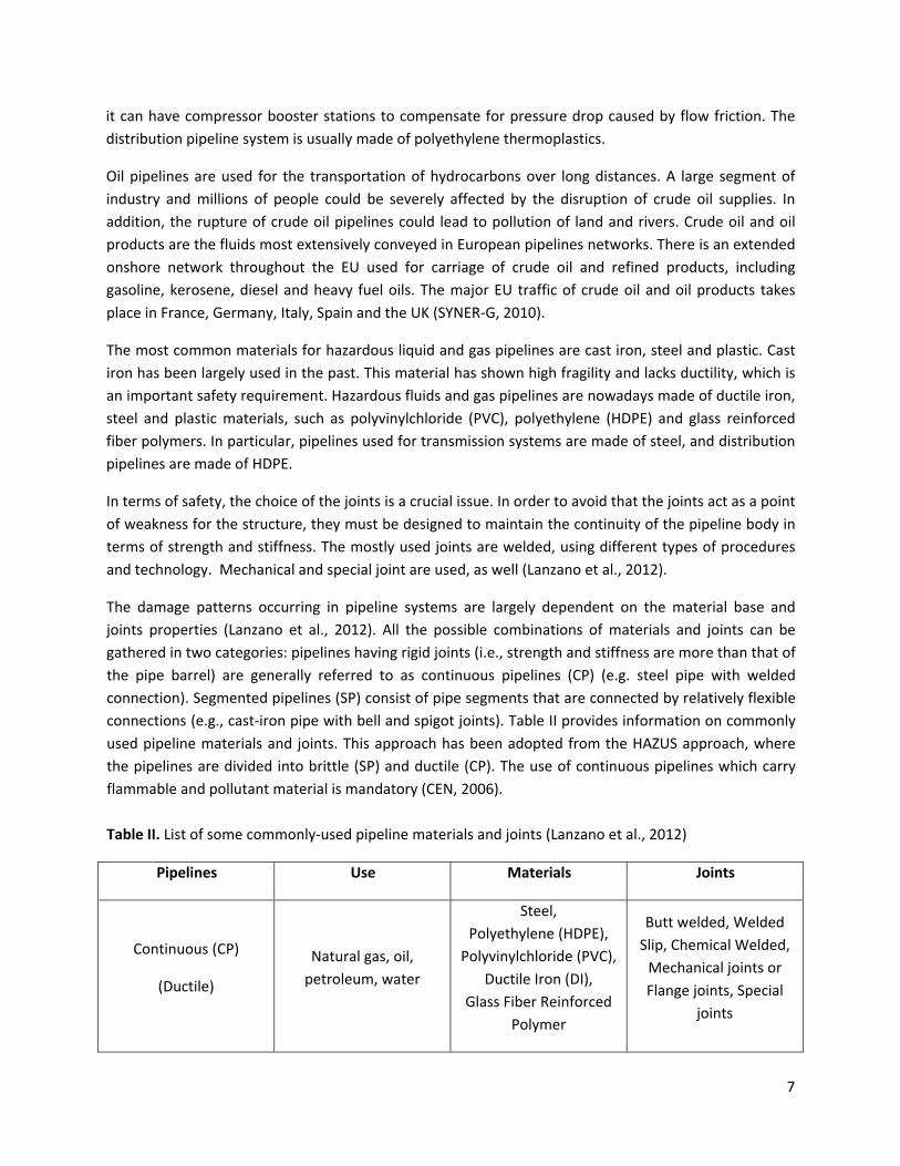
The  damage  patterns  occurring  in  pipeline  systems  are  largely  dependent  on  the material  base  and joints properties  (Lanzano  et  al.,  2012). All  the possible  combinations of materials  and  joints  can be gathered in two categories: pipelines having rigid joints (i.e., strength and stiffness are more than that of the  pipe  barrel)  are  generally  referred  to  as  continuous  pipelines  (CP)  (e.g.  steel  pipe with welded connection). Segmented pipelines (SP) consist of pipe segments that are connected by relatively flexible connections (e.g., cast‐iron pipe with bell and spigot joints). Table II provides information on commonly used pipeline materials and  joints. This approach has been adopted from the HAZUS approach, where the pipelines are divided  into brittle (SP) and ductile (CP). The use of continuous pipelines which carry flammable and pollutant material is mandatory (CEN, 2006).  Table II. List of some commonly‐used pipeline materials and joints (Lanzano et al., 2012) 

Pipelines  Use  Materials  Joints 

Continuous (CP) 

(Ductile) 

Natural gas, oil, petroleum, water 

Steel, Polyethylene (HDPE), Polyvinylchloride (PVC), 

Ductile Iron (DI), Glass Fiber Reinforced 

Polymer  

Butt welded, Welded Slip, Chemical Welded, Mechanical joints or Flange joints, Special 

joints 

  7

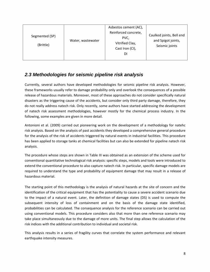
Segmented (SP) 

(Brittle) Water, wastewater 

Asbestos cement (AC), Reinforced concrete, 

PVC, Vitrified Clay, Cast Iron (CI),  

DI 

Caulked joints, Bell end and Spigot joints, Seismic joints 

 

2.3 Methodologies for seismic pipeline risk analysis

Currently,  several authors have developed methodologies  for  seismic pipeline  risk analysis. However, these frameworks usually refer to damage probability only and overlook the consequences of a possible release of hazardous materials. Moreover, most of these approaches do not consider specifically natural disasters as the triggering cause of the accidents, but consider only third party damage, therefore, they do not really address natech risk. Only recently, some authors have started addressing the development of  natech  risk  assessment methodologies,  however mostly  for  the  chemical  process  industry.  In  the following, some examples are given in more detail. 

Antonioni et al.  (2009) carried out pioneering work on  the development of a methodology  for natehc risk analysis. Based on the analysis of past accidents they developed a comprehensive general procedure for the analysis of the risk of accidents triggered by natural events in industrial facilities. This procedure has been applied to storage tanks at chemical facilities but can also be extended for pipeline natech risk analysis. 

The procedure whose steps are shown in Table III was obtained as an extension of the scheme used for conventional quantitative technological risk analysis: specific steps, models and tools were introduced to extend the conventional procedure to also capture natech risk. In particular, specific damage models are required to understand the type and probability of equipment damage that may result  in a release of hazardous material.  The starting point of this methodology  is the analysis of natural hazards at the site of concern and the identification of the critical equipment that has the potentiality to cause a severe accident scenario due to  the  impact of a natural event.  Later,  the definition of damage  states  (DS)  is used  to  compute  the subsequent  intensity  of  loss  of  containment  and  on  the  basis  of  the  damage  state  identified, probabilities can be calculated. The consequence analysis for the reference scenario can be carried out using conventional models. This procedure considers also that more than one reference scenario may take place simultaneously due to the damage of more units. The final step allows the calculation of the risk indices with the additional contribution to individual and societal risk. 

This analysis  results  in a  series of  fragility curves  that correlate  the  system performance and  relevant earthquake intensity measures.  

  8

Table III. Steps of the general procedure developed for the analysis of the risk induced by natural events in process facilities (Antonioni et al., 2009) 

Nr.  Steps  Needs 

1  Characterization of the external event  Frequency and severity parameters 

2  Identification of target equipment  List of target equipment considered 

3  Identification of damage states and reference scenarios  Event trees  

4  Estimation of the damage probability   Equipment damage models 

5  Consequence evaluation of the reference scenario  Consequence analysis models 

6  Identification of credible combinations of events  Set of event combinations 

7  Frequency/probability calculation for each combination  Frequency of event combinations 

8  Consequence calculation for each combination  Overall vulnerability map 

9  Calculation of risk indices  Overall risk indices 

 

Santella et al. (2011) suggest an empirical estimation of the conditional probability of natech events with respect  to  different  possible  kinds  of  natural  disasters:  i.e.,  hurricanes,  earthquakes,  tornadoes,  and floods at facilities covered by the US Toxic Release Inventory Program, the Risk Management Program, and  onshore  facilities  engaged  in  oil  and  gas  extraction  (SIC  1311).  Concerning  earthquakes,  natech accidents are analyzed considering the area impacted by the disaster. This area is then divided into one or more hazard zones based on the intensity of the hazard conditions experienced, i.e., Mercalli shaking intensity. Subsequently,  the number of  releases within each zone, aggregated by  type of  facility  from which the releases occurred, are pooled to estimate the conditional probability of the release under the particular natural event. The results are shown as curves describing  the probability of natech releases versus PGA. 

Recently,  Busini  et  al.  (2012)  proposed  a  short  cut methodology  for  the  analysis  of  industrial  risks induced  by  earthquakes.  The  idea  underpinning  this method  is  to  reduce  the  amount  of  time  and expertise required in a traditional Quantitative Risk Analysis (QRA),  trying to summarize in suitable Key Hazard  Indicators  (KHIs)  the  natech  risk  level  associated with  a  given  situation  (i.e.,  a  process  plant located at a given position). The aim of such screening procedure is to answer a simple question: ”Is the natech risk level associated with process plant A larger than the risk level associated with process plant B?”. Answering  this  question  requires  simultaneous  comparisons  among  a  large  number  of  different parameters, ranging from the type of hazardous substances present in the plant to the intensity of the external force, i.e., earthquake, each of which have different units of measurement. In order to evaluate the  different  risk  levels  corresponding  to  different  individual  risks  using  similar  units,  a  short‐cut methodology for the comparison and  integration of natural hazards and suitable  industrial risk  indices 

  9

was developed. The Analytical Hierarchy Process was chosen to support decision making by establishing alternatives  within  a  framework  of multi‐weighted  criteria:  it  allows  for  a  rational  choice  between alternatives on the basis of binary comparisons, i.e., comparisons involving only two elements at a time. Simple  algebraic  manipulations  of  these  binary  comparisons  determine  the  weight  for  the  various branches of  the hierarchy. At  the bottom of  the hierarchy  there are  the alternatives  that characterize the given plant with respect to the natech hazard. The consequences of the earthquake–related natech accidents are grouped into 3 main phenomena, and consequently three different hierarchies leading to 3 distinct indices related to fire, explosions and toxic dispersion. To determine the hazard level of a given plant, the three values are condensed into a global KHI which represents the overall hazard level in the KHI space. 

2.3.1 Pipeline damage due to earthquakes 

Underground  pipelines  and  above‐ground  facilities  present  considerably  different  seismic  response behaviors. Although buried structures are generally considered  less vulnerable  to seismic events  than above‐ground  structures,  severe  consequences on underground pipelines were observed due  to past strong  seismic  events.  The  seismic  response  of  pipelines  is  dominated  by  soil  deformation,  so  that vulnerability  assessment  strongly  depends  on  the  ground  response  evaluation:  since  the  relative movement of pipes with  respect  to  the  surrounding  soil  is generally  small,  the  structural  response  is dominated by the surrounding soil behavior (Scandella, 2007).  

Scandella (2007) also notes that underground pipelines tend to move with the ground instead of vibrate independently  and, due  to  their development  in  extended  areas,  the  space  variability of  the  seismic shaking plays a  relevant  role. As a consequence,  it can be assumed  that  the  structure  is  subjected  to free‐field stresses and strains due to the motion of the surrounding soil, while the relative movement of the structure with respect to the soil is generally negligible. 

The seismic response of buried structures is usually described through displacements and deformations induced  in  the  surrounding  soil.  Seismic  effects  are  generally  grouped  in  permanent  ground deformations  (PGD) and transient ground deformations  (TGD). PGD typically occur  in  isolated areas of ground failure and they may be associated either to the direct seismic effects of surface faulting, or the induced effects of landslides, seismic settlement, and lateral spreading due to soil liquefaction. Transient ground deformations are due to the passage of seismic waves associated with strong shaking (Scandella, 2007). Transient effects, common to all earthquakes, are felt over a large geographical area and, even if the resulting damage is relative low if compared with the high damage rates due to permanent ground deformations,  it may  be  relevant.  The  relative  impact  of  different  effects  varies  from  earthquake  to earthquake. There have been  some events where  lifeline damage occurred due  to wave propagation alone. An  example  is  the  significant  pipeline  and  tunnel  damage  in Mexico  City  caused  by  the  1985 Michoacan earthquake (Ayala and M.J. O’Rourke, 1989). 

Typically, damage occurs due to a combination of effects. For  instance, during the 1906 San Francisco event roughly half of the pipe breaks occurred within liquefaction‐induced lateral spreading zones while the  other  half  occurred  over  a  somewhat  larger  area where wave  propagation was  apparently  the 

  10

dominant cause (O’Rourke et al., 1992). The same pattern was observed after the 1999 Chi‐Chi (Taiwan) event, when  the water pipeline damage  revealed  the  relative  impact of different earthquake effects: half of the total damage was related to ground shaking, damage was also high (35 %) due to extensive faulting and  large  fault displacements,  landslides were  responsible  for 11% of  the damage because of the mountainous affected area, whereas liquefaction damage was relatively insignificant (2%) (Miyajima and Hashimoto, 2001). 

The  response  of  underground  structures  depends  on  various  factors  including  the  intensity  of  the earthquake,  the  geological  conditions,  the  structure’s  location  with  respect  to  the  fault  (e.g.  fault‐crossing) or the structure’s axis alignment with respect to the propagation direction of the wave field, and the structure’s properties such as shape, extension, depth and mechanical‐structural characteristics, which influence the strain state and the potential damage. 

General observations can be made regarding the seismic performance of underground facilities, based on earthquake damage  incurred by  infrastructures during past earthquakes. Hashash et al.  (2001)  list the following points: 

1. Underground structures suffer  less damage than surface structures due to the confining pressure of the surrounding soil and the decreasing of the maximum displacements and accelerations with depth; 

2. The response of underground  lifelines  is dominated by the surrounding ground response and not by the inertial properties on the structure itself; 

3. The reported damage decreases with increasing depth of the soil layer above the infrastructure; 

4. Underground facilities constructed  in soft soils are expected to suffer more damage with respect to those in rock; 

5. Lined and reinforced structures are less vulnerable than unlined and non‐reinforced ones; stabilizing the surrounding soil and improving the soil‐structure contact can reduce shaking damage; 

6.  Underground  lifelines  are  more  stable  under  symmetric  load  as  it  improves  the  ground‐lining interaction; 

7. Damage may be related to parameters which can be evaluated easily, such as PGA or PGV; 

8. The duration of the seismic event is of crucial importance, because a long strong‐motion shaking can cause fatigue failure; 

9. Ground motion may be  amplified upon  incidence with  a  structure  if  incident wavelengths  are 2‐4 times the facility diameter. 

In  a  seismic  event,  continuous  and  segmented  pipelines  have  different  failure  modes.  Continuous pipelines  often  fail  due  to  tensile  rupture,  local  buckling  and  beam  buckling.  The  failure modes  of segmented pipelines, especially of those with  large diameters and thick walls, are tensile  failure  (axial pull‐out),  compression  failure  (crushing  of  joints),  and  circumferential  flexure  and  joint  rotation.  In 

  11

segmented pipeline,  failures are concentrated at  the  joints, however, continuous pipelines mainly  fail due  to  the  rupture  of  pipe  barrel.  For  a  detailed  description  of  the  different  failure modes  of  both continuous and segmented pipelines the reader is referred to Dash and Jain (2007).  Studies based on  the  recorded number of  repairs during past  earthquakes do not  always distinguish between  leaks and breaks of  the pipes. As a  result, all  fragility  relations  for pipelines are given  for a single “failure” e.g.,  the  repair  rate  (RR) per unit  length of pipe. However, according  to HAZUS  (NIBS, 2004a), the type of repair or damage depends on the type of hazard: a pipe damaged because of ground failure  is  likely  to  present  a  break, whereas  ground  shaking may  induce more  leak‐related  damage. Based on these assumptions, HAZUS defines 3 categories of damage states (DS) (Table IV):  Table IV.  Proposed damage states for pipelines (NIBS, 2004a) 

  Damage state  Damage description  Serviceability 

DS1  no damage  no break/leak  operational 

DS2  leakage  at least one leak along the pipe length  reduction of the flow 

DS3  failure  at least one break along the pipe length  disruption of the flow 

2.3.2 Fragility estimation 

A seismic fragility model describes the performance of an engineering component or system subject to earthquake excitations in probabilistic terms (Straub and Der Kiureghian,2007). Fragility models are used to estimate the risk of the earthquake hazard acting on the components of  lifeline systems such as oil, water  and  gas  pipelines,  electric  power  distribution  systems,  transportation  networks  and  building systems. They are obtained either from statistical analysis of observed failures during past earthquakes (the empirical approach) or  from  structural modeling of  the  seismic performance of components and systems (Straub and Der Kiureghian, 2007). 

Several approaches can be used to establish the fragility curves. They can be grouped under empirical, expert‐judgment  based,  analytical  and  hybrid  (Rossetto  and  Eknashai,  2003).  Empirical methods  are based on the observation of actual damage and on past earthquake surveys. They have the advantage of being based on real observed data and therefore consider seismo‐tectonic and geotechnical conditions, as well as the characteristics of damaged structures. However, this means that these curves are specific to a particular site. 

Expert‐judgment  based  fragility  curves  rely  on  expert  opinion  and  experience.  Therefore,  they  are versatile and relatively  fast to derive, but their reliability  is uncertain because of their dependence on the experiences of the experts consulted. 

Analytical  fragility  curves  are based on  the estimation of  the damage distributions  that  are obtained through the simulation of an element’s structural response subjected to seismic action. This can result in a reduced bias and increased reliability of the vulnerability estimates for different structures compared 

  12

to  expert  opinion  (Rossetto  and  Elnashai,  2003).  Analytical  approaches  are  becoming  ever  more attractive in terms of the ease and efficiency by which data can be generated. 

Hybrid curves combine any of the above‐mentioned techniques. 

The study of past earthquakes and field surveys of actual damage of exposed elements allow compiling extensive statistics on the damage states of various typologies under earthquake loading. For instance, the  study  by  Spence  et  al.  (1992)  yielded  fragility  curves  for  14  classes  of  buildings,  expressed  as functions of macroseismic intensity. These results are based on a survey of 70.000 buildings subjected to 13 different earthquakes. Sabetta et al.  (1998) also developed empirical  fragility curves after studying data of 50.000 Italian buildings. The probability of exceeding a damage state is expressed with respect to PGA or spectral response parameters, which are converted from the observed macroseismic intensity. A similar work was  performed  by Rota  et  al.  (2006)  on  Italian  buildings.  Finally, Rossetto  and  Elnashai (2003) developed empirical  functions  for various  typologies of RC buildings  (moment‐resisting  frames, infill walls,  shear walls)  from  a  database  of  340,000  buildings  exposed  to  19  earthquakes.  Empirical relations are also widely used to assess the vulnerability of components that are less prone to analytical developments  than  buildings,  e.g.  pipeline  segments  (ALA,  2001)  or  tunnels  (Corigliano,  2007)  and highway embankments (Maruyama, 2010). 

A distinction can also be made between direct methods that yield fragility curves as a function of ground motion  intensity measure  types  (e.g.  PGA,  PGV,  Sa(T),  etc.)  and  indirect methods  that  estimate  the damage probability with  respect  to  structural  response parameters  (e.g.  spectral displacement at  the inelastic  period).  The  latter  approach,  used  for  instance  in  the  framework  of  HAZUS  (NIBS,  2004a) requires for each seismic scenario computation of the structural response with the capacity curve, and then evaluation of the damage probability using the associated fragility curves. 

2.3.2.1 State­of­the­art of fragility curves for pipelines 

In  the  following  a  state‐of‐the‐art  of  fragility  curves  for  pipelines  is  presented.  Depending  on geotechnical dynamics effects related to the pipeline damage, pipeline fragility relations are subdivided into two categories: ground failure (GF) and ground shaking (SGS) effects. 

Seismic damage to pipelines is generally described through curves in which the performance indicator is expressed  as  a  function  of  seismic  intensity measure  (intensity  index  in  Table  V).  The  performance indicator for pipeline damage due to the earthquake is generally given in the literature as “repair rate”, “damage rate” or “damage ratio”; other studies use the term “failure rate”.  

Ground shaking effects (SGS) 

Based  on  the  literature  review  a  total  of  twenty‐six  authoritative  empirical  studies  relating  pipeline damage to SGS effects were selected. A summary of these studies is displayed in Table V along with the strong motion parameter(s) used to describe the earthquake effect, the characteristics of pipelines and the number of earthquakes from which data have been obtained in each study. In addition, the reader is 

  13

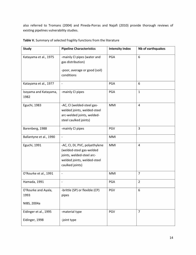
also  referred  to  Tromans  (2004)  and  Pineda‐Porras  and  Najafi  (2010)  provide  thorough  reviews  of existing pipelines vulnerability studies.   Table V. Summary of selected fragility functions from the literature 

Study  Pipeline Characteristics  Intensity Index  Nb of earthquakes 

Katayama et al., 1975  ‐mainly CI pipes (water and gas distribution) 

‐poor, average or good (soil) conditions 

PGA  6 

Katayama et al., 1977  ‐  PGA  6 

Isoyama and Katayama, 1982 

‐mainly CI pipes  PGA  1 

Eguchi, 1983  ‐AC, CI (welded‐steel gas‐welded joints, welded‐steel arc‐welded joints, welded‐steel caulked joints)  

MMI  4 

Barenberg, 1988  ‐mainly CI pipes  PGV  3 

Ballantyne et al., 1990  ‐  MMI   

Eguchi, 1991  ‐AC, CI, DI, PVC, polyethylene (welded‐steel gas‐welded joints, welded‐steel arc‐welded joints, welded‐steel caulked joints) 

MMI  4 

O’Rourke et al., 1991   ‐  MMI  7 

Hamada, 1991  ‐  PGA  2 

O’Rourke and Ayala, 1993 

NIBS, 2004a 

‐brittle (SP) or flexible (CP) pipes 

PGV  6 

Eidinger et al., 1995 

Eidinger, 1998 

‐material type 

‐joint type 

PGV  7 

  14

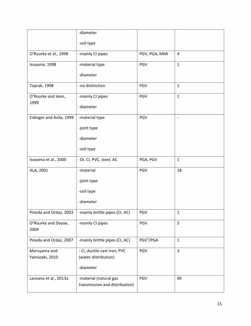
‐diameter 

‐soil type 

O’Rourke et al., 1998  ‐mainly CI pipes  PGV, PGA, MMI  4 

Isoyama, 1998  ‐material type  

‐diameter 

PGV   1 

Toprak, 1998  ‐no distinction  PGV  1 

O’Rourke and Jeon, 1999 

‐mainly CI pipes 

‐diameter 

PGV  1 

Eidinger and Avila, 1999  ‐material type 

‐joint type 

‐diameter 

‐soil type 

PGV  ‐ 

Isoyama et al., 2000  ‐DI, CI, PVC, steel, AC  PGA, PGV  1 

ALA, 2001  ‐material 

‐joint type 

‐soil type 

‐diameter 

PGV  18 

Pineda and Ordaz, 2003  ‐mainly brittle pipes (CI, AC)  PGV  1 

O’Rourke and Deyoe, 2004 

‐mainly CI pipes  PGV  5 

Pineda and Ordaz, 2007  ‐mainly brittle pipes (CI, AC)  PGV2/PGA  1 

Maruyama and Yamazaki, 2010 

‐ CI, ductile cast iron, PVC (water distribution) 

‐diameter 

PGV  3 

Lanzano et al., 2013a  ‐material (natural gas transmission and distribution) 

PGV  40 

  15

‐joint type 

‐diameter  

Lanzano et al., 2013b  continuous pipelines (CP), segmented pipelines (SP) 

PGV, PGA  20 

 

In the following, a summary of selected empirical relations is provided.  

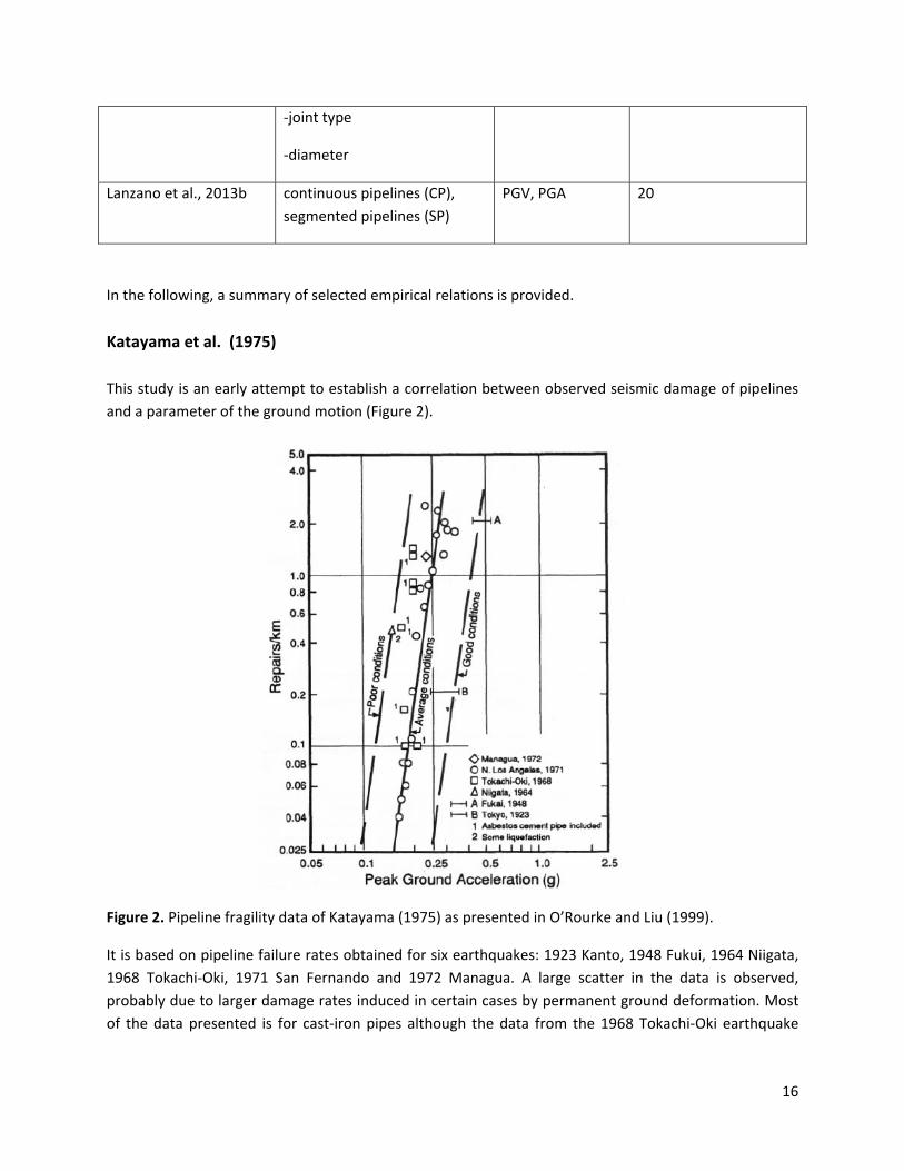
Katayama et al.  (1975)  This study is an early attempt to establish a correlation between observed seismic damage of pipelines and a parameter of the ground motion (Figure 2). 

 

Figure 2. Pipeline fragility data of Katayama (1975) as presented in O’Rourke and Liu (1999). 

It is based on pipeline failure rates obtained for six earthquakes: 1923 Kanto, 1948 Fukui, 1964 Niigata, 1968  Tokachi‐Oki,  1971  San  Fernando  and  1972 Managua.  A  large  scatter  in  the  data  is  observed, probably due to larger damage rates induced in certain cases by permanent ground deformation. Most of  the data presented  is  for cast‐iron pipes although  the data  from  the 1968 Tokachi‐Oki earthquake 

  16

includes damage to asbestos‐cement pipes. No distinction is made between pipe diameters, joint types or pipe material. However, in the fragility relationship Eq. (1),   

PGAbRR log39.610 +=                                                                           (1)  a parameter b is introduced which depends on several factors like soil condition or pipe age. Depending on  the  “poor”,  “average”  or  “good”  conditions,  this  constant  can  take  the  values  4.75,  3.65  or  2.0, respectively (Ayala and Rourke, 1989). RR is the repair rate per km.  

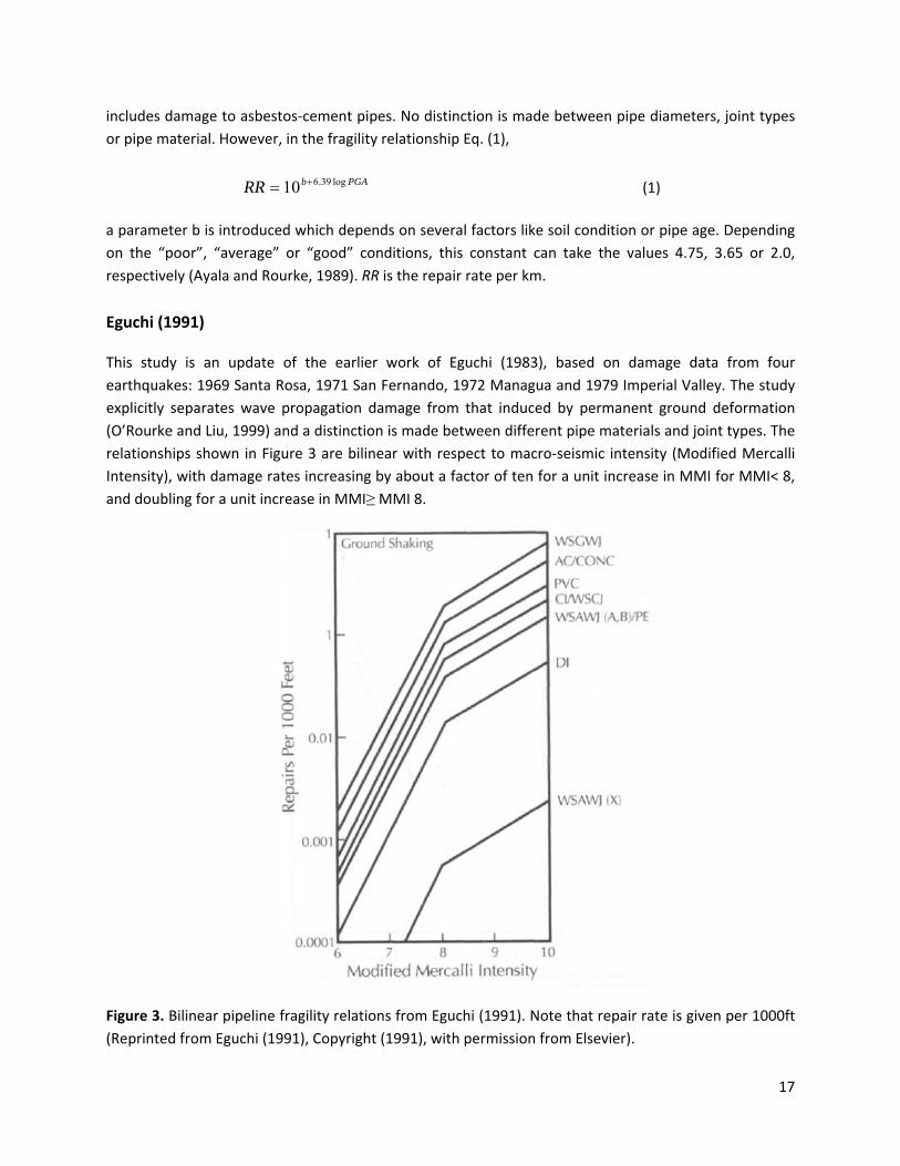
Eguchi (1991)  This  study  is  an  update  of  the  earlier  work  of  Eguchi  (1983),  based  on  damage  data  from  four earthquakes: 1969 Santa Rosa, 1971 San Fernando, 1972 Managua and 1979 Imperial Valley. The study explicitly  separates wave propagation  damage  from  that  induced by  permanent  ground  deformation (O’Rourke and Liu, 1999) and a distinction is made between different pipe materials and joint types. The relationships shown  in Figure 3 are bilinear with respect to macro‐seismic  intensity  (Modified Mercalli Intensity), with damage rates increasing by about a factor of ten for a unit increase in MMI for MMI< 8, and doubling for a unit increase in MMI≥ MMI 8. 

 

Figure 3. Bilinear pipeline fragility relations from Eguchi (1991). Note that repair rate is given per 1000ft (Reprinted from Eguchi (1991), Copyright (1991), with permission from Elsevier). 

  17

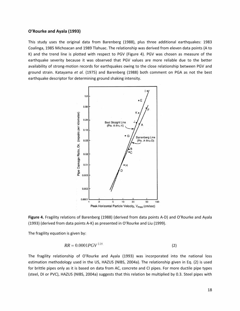
O’Rourke and Ayala (1993)  This  study  uses  the  original  data  from  Barenberg  (1988),  plus  three  additional  earthquakes:  1983 Coalinga, 1985 Michoacan and 1989 Tlahuac. The relationship was derived from eleven data points (A to K)  and  the  trend  line  is  plotted with  respect  to  PGV  (Figure  4).  PGV was  chosen  as measure  of  the earthquake  severity  because  it  was  observed  that  PGV  values  are more  reliable  due  to  the  better availability of strong‐motion records for earthquakes owing to the close relationship between PGV and ground  strain.  Katayama  et  al.  (1975)  and Barenberg  (1988)  both  comment  on  PGA  as  not  the  best earthquake descriptor for determining ground shaking intensity. 

 

Figure 4. Fragility relations of Barenberg (1988) (derived from data points A‐D) and O’Rourke and Ayala (1993) (derived from data points A‐K) as presented in O’Rourke and Liu (1999). 

The fragility equation is given by:  

25.20001.0 PGVRR =                                                                       (2)     The  fragility  relationship  of  O’Rourke  and  Ayala  (1993)  was  incorporated  into  the  national  loss estimation methodology used  in the US, HAZUS (NIBS, 2004a). The relationship given  in Eq. (2)  is used for brittle pipes only as it is based on data from AC, concrete and CI pipes. For more ductile pipe types (steel, DI or PVC), HAZUS (NIBS, 2004a) suggests that this relation be multiplied by 0.3. Steel pipes with 

  18

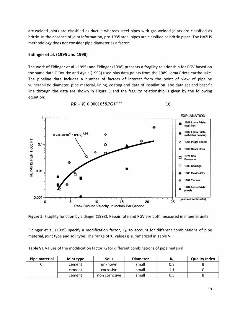
arc‐welded  joints are  classified as ductile whereas  steel pipes with gas‐welded  joints are  classified as brittle. In the absence of joint information, pre‐1935 steel pipes are classified as brittle pipes. The HAZUS methodology does not consider pipe diameter as a factor.  Eidinger et al. (1995 and 1998)  The work of Eidinger et al. (1995) and Eidinger (1998) presents a fragility relationship for PGV based on the same data O’Rourke and Ayala (1993) used plus data points from the 1989 Loma Prieta earthquake. The  pipeline  data  includes  a  number  of  factors  of  interest  from  the  point  of  view  of  pipeline vulnerability: diameter, pipe material,  lining, coating and data of  installation. The data set and best‐fit line  through  the  data  are  shown  in  Figure  5  and  the  fragility  relationship  is  given  by  the  following equation: 

98.11 0001658.0 PGVKRR =                                             (3) 

 

 

Figure 5. Fragility function by Eidinger (1998). Repair rate and PGV are both measured in imperial units  

Eidinger  et  al.  (1995)  specify  a modification  factor, K1,  to  account  for different  combinations of pipe material, joint type and soil type. The range of K1 values is summarized in Table VI.  Table VI. Values of the modification factor K1 for different combinations of pipe material 

 Pipe material  Joint type  Soils  Diameter  K1  Quality Index 

cement  unknown  small  0.8  B cement  corrosive  small  1.1  C 

CI 

cement  non corrosive  small  0.5  B 

  19

rubber gasket  unknown  small  0.5  D arc welded  unknown  small  0.5  C arc welded  corrosive  small  0.8  D arc welded  Non corrosive  small  0.3  B arc welded  all  large  0.15  B 

WS 

rubber gasket  unknown  small  0.7  D rubber gasket  all  small  0.5  C 

cement  all  small  1.0  B AC cement  all  large  2.0  D welded  all  large  1.0  D 

C cement  all  large  2.0  D 

PVC  rubber gasket  all  small  0.5  C DI  rubber gasket  non corrosive  all  0.3  C 

  For the diameter values, “small” refers to pipe diameters D< 30.48 cm (12 inches); “large” refers to D ≥ 30.48 cm. Each K1 value is classified according to a data quality index, which describes the confidence in the current empirical data set. Each level has an approximate qualitative description: B ‐ "there is a reasonable amount of backup empirical data and study" C ‐ "limited empirical data and study" D ‐ "based largely on extrapolation and judgment, with very limited empirical data". 

 Isoyama et al. (2000)   The work of Isoyama et al. (2000) is based on earlier studies of the 1995 Kobe earthquake.  The pipeline fragility relationships were derived using the following functional forms (Eqs. (4) and (5)):  

( ) ( )IMRCCCCIMR lgdpm ⋅⋅⋅⋅=   (4) 

where Rm(IM) is the pipeline repair rate per km of pipe as a function of the intensity measure  parameter IM,  Cp, Cd, Cg, and Cl are correction coefficients for the pipe material, diameter, geological condition, and liquefaction occurrence, respectively. IM is the peak ground velocity (PGV) and R(IM) estimates the damage ratio for cast‐iron pipes with a certain diameter: 

( bIMIMaIMR min)( −= )                                                             (5) 

Parameters a and b are regression coefficients and IMmin is the minimum value of strong ground motion for which damage  is  considered  to occur. The  repair  rate  as  a  function of PGA  and PGV  is  shown  in Figures 6a and 6b, respectively. The  fragility relations are based on 19 data points and 16 data points respectively. In each case, several additional outlying points were excluded due to extreme instances of liquefaction or topographic effects. 

  20

 

Figure 6.  Data sets and fragility relations from Isoyama et al. (2000); a) acceleration scale is PGA (1gal = 1cm/s2); b)  velocity  scale  is PGV  (1  kine  = 1cm/s).  Solid  squares  indicate data points  included  in  the regression while. Open squares indicate outliers excluded from the data set.  

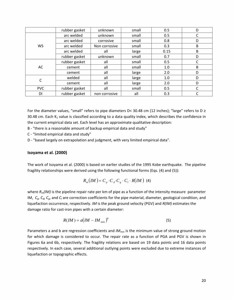
ALA (2001)  In 2001,  the American Lifelines Alliance  (ALA), published a  set of detailed procedures  to evaluate  the probability of damage from earthquake effects to various components of the water supply system (ALA, 2001).  In  the  work  were  included  water  distribution  systems  (pipelines,  tunnels  and  canals), aboveground  cylindrical  storage  tanks  and  portions  of  the  conveyance  control  and  data  acquisition system (SCADA) that are located along the conveyance system, and flow control mechanisms (e.g. valves and gates). For each  component,  the  likely damage  states and  corresponding  fragility  functions were presented.  For  buried  pipelines,  fragility  relations were  developed  separately  for  permanent  ground deformation effects and ground shaking effects. For each data point, pipe material, pipe repair rate (RR), pipe diameter, PGV and are  specified. Pipe material and pipe diameter  categories are  summarized  in Table VII and the full data set of ALA is presented in Figure 7.  Table  VII.  Pipe  characteristics  included  in  the  dataset  for  ALA  (2001)  fragility  relation  (percentage subject to rounding errors). 

 

  21

 

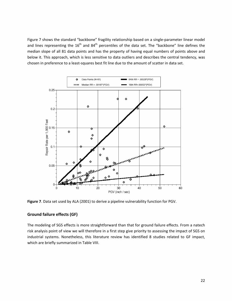
Figure 7 shows the standard “backbone” fragility relationship based on a single‐parameter linear model and  lines  representing  the 16th and 84th percentiles of  the data  set. The  “backbone”  line defines  the median slope of all 81 data points and has the property of having equal numbers of points above and below it. This approach, which is less sensitive to data outliers and describes the central tendency, was chosen in preference to a least‐squares best fit line due to the amount of scatter in data set.  

 

Figure 7. Data set used by ALA (2001) to derive a pipeline vulnerability function for PGV.  

Ground failure effects (GF) 

The modeling of SGS effects is more straightforward than that for ground failure effects. From a natech risk analysis point of view we will therefore in a first step give priority to assessing the impact of SGS on industrial  systems. Nonetheless,  this  literature  review  has  identified  8  studies  related  to GF  impact, which are briefly summarized in Table VIII.     

  22

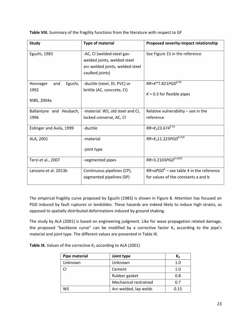
Table VIII. Summary of the fragility functions from the literature with respect to GF 

Study  Type of material  Proposed severity‐impact relationship 

Eguchi, 1983  ‐AC, CI (welded‐steel gas‐welded joints, welded‐steel arc‐welded joints, welded‐steel caulked joints) 

See Figure 15 in the reference 

Honneger  and  Eguchi, 1992 

NIBS, 2004a 

‐ductile (steel, DI, PVC) or brittle (AC, concrete, CI) 

RR=K*7.821PGD0.56 

K = 0.3 for flexible pipes 

Ballantyne  and  Heubach, 1996 

‐material: WS, old steel and CI, locked converse, AC, CI 

Relative vulnerability – see in the reference 

Eidinger and Avila, 1999  ‐ductile  RR=K223.6740.53 

ALA, 2001  ‐material 

‐joint type 

RR=K211.223PGD0.319 

Terzi et al., 2007  ‐segmented pipes  RR=3.2103PGD0.4103 

Lanzano et al. 2013b  Continuous pipelines (CP), segmented pipelines (SP) 

RR=aPGDb – see table 4 in the reference for values of the constants a and b 

 

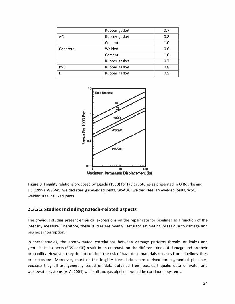
The empirical fragility curve proposed by Eguchi (1983)  is shown  in Figure 8. Attention has focused on PGD  induced by  fault ruptures or  landslides. These hazards are  indeed  likely to  induce high strains, as opposed to spatially distributed deformations induced by ground shaking. 

The study by ALA (2001) is based on engineering judgment. Like for wave propagation related damage, the  proposed  “backbone  curve”  can  be modified  by  a  corrective  factor  K2  according  to  the  pipe’s material and joint type. The different values are presented in Table IX. 

Table IX. Values of the corrective K2 according to ALA (2001) 

Pipe material   Joint type  K2 

Unknown  Unknown  1.0 

Cement  1.0 

Rubber gasket  0.8 

CI 

Mechanical restrained  0.7 

WS  Arc‐welded, lap welds  0.15 

  23

Rubber gasket  0.7 

Rubber gasket  0.8 AC 

Cement  1.0 

Welded  0.6 

Cement  1.0 

Concrete 

Rubber gasket  0.7 

PVC  Rubber gasket  0.8 

DI  Rubber gasket  0.5 

 

 

Figure 8. Fragility relations proposed by Eguchi (1983) for fault ruptures as presented in O’Rourke and Liu (1999). WSGWJ: welded steel gas‐welded joints, WSAWJ: welded steel arc‐welded joints, WSCJ: welded steel caulked joints 

2.3.2.2 Studies including natech­related aspects 

The previous studies present empirical expressions on the repair rate for pipelines as a function of the intensity measure. Therefore, these studies are mainly useful for estimating  losses due to damage and business interruption.  

In  these  studies,  the  approximated  correlations  between  damage  patterns  (breaks  or  leaks)  and geotechnical aspects  (SGS or GF) result  in an emphasis on  the different kinds of damage and on  their probability. However, they do not consider the risk of hazardous‐materials releases from pipelines, fires or  explosions.  Moreover,  most  of  the  fragility  formulations  are  derived  for  segmented  pipelines, because  they  all  are  generally  based  on  data  obtained  from  post‐earthquake  data  of  water  and wastewater systems (ALA, 2001) while oil and gas pipelines would be continuous systems.  

  24

Due  to  these  limitations,  the natech risk assessment of pipelines  requires  further model development and fragility formulations based on different specific indicators, the specific level of damage and specific curves for each type of geotechnical and structural pipeline aspect (Lanzano et al., 2012). 

Four studies addressing natech risk in pipelines are discussed in more detail in the following. 

Lanzano et al. (2012, 2013b)  

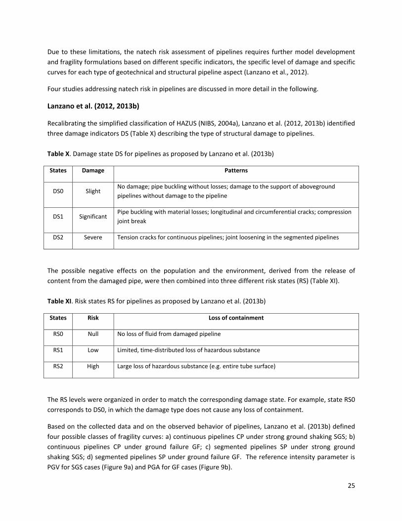
Recalibrating the simplified classification of HAZUS (NIBS, 2004a), Lanzano et al. (2012, 2013b) identified three damage indicators DS (Table X) describing the type of structural damage to pipelines.  Table X. Damage state DS for pipelines as proposed by Lanzano et al. (2013b) 

States  Damage  Patterns 

DS0  Slight No damage; pipe buckling without losses; damage to the support of aboveground pipelines without damage to the pipeline 

DS1  Significant Pipe buckling with material losses; longitudinal and circumferential cracks; compression joint break 

DS2  Severe  Tension cracks for continuous pipelines; joint loosening in the segmented pipelines 

 

The  possible  negative  effects  on  the  population  and  the  environment,  derived  from  the  release  of content from the damaged pipe, were then combined into three different risk states (RS) (Table XI).  Table XI. Risk states RS for pipelines as proposed by Lanzano et al. (2013b) 

States  Risk  Loss of containment 

RS0  Null  No loss of fluid from damaged pipeline 

RS1  Low  Limited, time‐distributed loss of hazardous substance 

RS2  High  Large loss of hazardous substance (e.g. entire tube surface) 

 

The RS levels were organized in order to match the corresponding damage state. For example, state RS0 corresponds to DS0, in which the damage type does not cause any loss of containment.  

Based on the collected data and on the observed behavior of pipelines, Lanzano et al. (2013b) defined four possible classes of fragility curves: a) continuous pipelines CP under strong ground shaking SGS; b) continuous  pipelines  CP  under  ground  failure  GF;  c)  segmented  pipelines  SP  under  strong  ground shaking SGS; d) segmented pipelines SP under ground failure GF.   The reference  intensity parameter  is PGV for SGS cases (Figure 9a) and PGA for GF cases (Figure 9b).  

  25

 

Figure 9. Fragility curves for buried pipelines under SGS (a) and GF (b) in terms of limit state probability percentage for the RS state: □: CP RS ≥RS1; ◊: CP RS=RS2; ○: SP RS≥ RS1; ∆: SP RS=RS2 (Reprinted from Lanzano et al. (2013b), Copyright (2013), with permission from Elsevier).  

In addition, in order to obtain univocal threshold values both for PGV and PGA with reference to the RS states, the seismic vulnerability is also presented as a probit function (Figures 10a and b). 

 

Figure 10.Probit  curves  for buried pipelines under SGS  (a) and GF  (b). RS  state: □: CP RS  ≥RS1;  ◊: CP RS=RS2; ○:  SP  RS≥  RS1;  ∆:  SP  RS=RS2  (Reprinted  from  Lanzano  et  al.  (2013),  Copyright  (2013), with permission from Elsevier).  

Omidvar et al. 2013  These authors propose a damage analysis of buried fuel pipeline systems and assess the probability of consequences of hydrocarbon releases from the pipelines considering that the presence of aerial power 

  26

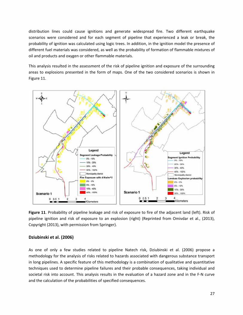
distribution  lines  could  cause  ignitions  and  generate  widespread  fire.  Two  different  earthquake scenarios were  considered  and  for  each  segment  of  pipeline  that  experienced  a  leak  or  break,  the probability of ignition was calculated using logic trees. In addition, in the ignition model the presence of different fuel materials was considered, as well as the probability of formation of flammable mixtures of oil and products and oxygen or other flammable materials. 

This analysis resulted in the assessment of the risk of pipeline ignition and exposure of the surrounding areas  to explosions presented  in  the  form of maps. One of  the  two considered  scenarios  is  shown  in Figure 11.  

 

Figure 11. Probability of pipeline leakage and risk of exposure to fire of the adjacent land (left). Risk of pipeline  ignition  and  risk of  exposure  to  an  explosion  (right)  (Reprinted  from Omivdar  et  al.,  (2013), Copyright (2013), with permission from Springer).  

Dziubinski et al. (2006)  As  one  of  only  a  few  studies  related  to  pipeline  Natech  risk,  Dziubinski  et  al.  (2006)  propose  a methodology for the analysis of risks related to hazards associated with dangerous substance transport in long pipelines. A specific feature of this methodology is a combination of qualitative and quantitative techniques used to determine pipeline failures and their probable consequences, taking  individual and societal risk  into account. This analysis results  in the evaluation of a hazard zone and  in the F‐N curve and the calculation of the probabilities of specified consequences. 

  27

Jo and Ahn (2005)  Jo  and  Ahn  (2005)  propose  a  risk  analysis  for  natural  gas  pipelines  in  terms  of  fatal  length  and cumulative fatal length. This analysis considers third party damage, among which earthquakes are listed, and studies their consequences on the population. Although the authors do not provide a relationship between  the  intensity measure  that describes  the  earthquake  and  the  consequences  (fragility  curve) they consider the consequences of releases in their work. 

3. Vulnerability of pipelines to floods 

Numerous  severe  accidents highlight  the  risk  associated with  floods  impacting pipelines  transporting dangerous  substances.  One  major  accident  in  the  San  Jacinto  River  Valley  in  1994  was  already mentioned in the introduction. 

More recently,  in June 2013, parts of Alberta  (Canada) were under a state of emergency because of a 100‐year flood event. Two pipeline leaks were directly linked to the heavy rains: in the Turner Valley, a pipeline  carrying  sour  gas  containing one per  cent hydrogen  sulfide was  ruptured by  floating debris, prompting the evacuation of residents within a 100‐mile radius. Although the operator Legacy Oil and Gas shut the line off from the source, it was impossible to access the line itself due to deepening flood waters (DeSmog Canada, 2013).  In northeast Alberta, the Canadian pipeline company Enbridge Energy closed its Wood Buffalo pipeline system in response to a spill from its line 37. About 730 barrels of crude oil spilled from line 37. Enbridge said that no potable water wells were affected by the release although some oil spilled into a small creek and a lake. There have been reported impacts from the flood involving exposed pipelines caused by erosion or rerouting of waterways (UPI, 2013). 

Floods are among  the most  frequent natural hazards  that  trigger  technological accidents  (Krausmann and Baranzini, 2012) and pipework was found to be very vulnerable to flood effects, often leading to loss of  containment  and  possible  reaction  of  the  released  chemicals  with  water  (Cozzani  et  al.,  2010). Nevertheless, only very few dedicated studies can be found on the impact of floods on pipelines in the scientific literature. This lack of studies can partially be ascribed to the fact that often “flooding” is seen as a secondary phenomenon, due to rain or other natural hazards, for example hurricanes. 

During floods, the extreme forces of the floodwaters, heavy floating debris, natural erosion and water pressure from high water can adversely affect pipelines. Moreover, flood waters change the landscape, and pipelines may become  susceptible  to damage:  for  instance, during  inspections  following pipeline ruptures  beneath  the  Yellowstone  River,  pipeline  operators  observed  that  the  river  seemed  to  be carving a deeper channel, leaving the arteries of the pipeline exposed (TRP, 2011).  

This topic is nowadays becoming a great concern due to the high frequency of severe flooding events. In 2011,  the  Pipeline  and  Hazardous  Materials  Safety  Administration  of  the  US  Department  of Transportation  issued  an  advisory  bulletin  to  all  owners  and  operators  of  gas  and  hazardous  liquid pipelines to communicate the potential for damage to pipeline facilities caused by severe flooding. This 

  28

advisory  includes  recommended  industrial  facility planning procedures  that operators should consider taking to ensure the integrity of pipelines in case of impending or extreme flooding (PHMSA, 2011).  Because of the scarcity of data specifically dedicated to pipelines, a review of the literature on damage of industrial items due to flood events is presented in the following sections.  

3.1 Flood severity measures

The consequences of flood damage in pipelines or industrial equipment are the results of the interaction of a number of flood characteristics with the system under study. The most important identified factors are:  water  depth,  flow  velocity,  duration  of  the  inundation  and  sediment  or  debris  load  and  the interaction of these factors with the system. 

The characterization of the flood event requires the assessment of frequency and severity of the floods. The  standard  parameter  for  the  frequency  is  the  return  period  (Tr) measured  in  years  and  given  by hydrological studies. Since there are different kinds of flood events, for example floodplain  inundation with high water  level or flash flood with high water velocity,  it  is necessary to distinguish the possible modalities  of  flood  impact  (slow  submersion, moderate  speed  wave,  high  speed  wave).  From  this standpoint,  the  flood  severity  can  be  quantified  by  two  parameters: water  depth  and water  speed. Nevertheless these parameters are usually not reported in general flood hazard assessment studies and are not available unless specific analyses were performed for a given site (Campedel et al., 2009).  

Numerical simulation can help to model the flood dynamics, by computing high flow velocities and high water level conditions which can be assumed as threshold limit values for structural damage with loss of containment and subsequent release of hazardous materials (DCP, 2003).  For instance, the value of the severity parameters allows the computation of the overall pressure acting on process equipment on the basis of hydrostatic pressure. 

3.2 Methodologies for pipeline risk analysis with respect to floods

Concerning  risk  analysis  with  respect  to  floods,  much  of  the  research  present  in  the  literature  is dedicated to housing risk assessment. Few studies address industrial plants (Su et al., 2009; Booysen et al., 1999), chemical plants (Campedel et al., 2009, RiskScape, 2005, Krausmann and Mushtaq, 2008), or natech risk analysis (Rota et al. 2008; Cozzani et al., 2010, Santella et al., 2011) and very little has been found  specifically applied to pipelines (NIBS, 2004b; Chisolm and Matthews, 2012). 

Three  general  frameworks  of  risk  analysis  related  to  floods  events  exist  in  the  literature  and  have already been introduced in section 2.3, applied to earthquakes.  They are 1) the empirical estimation of the  probability  of  a  natech  event,  as  e.g.  presented  in  Santella  et  al.  (2011),  2)  the  short‐cut methodology proposed in Busini et al. (2011) and applied in Rota et al. (2008) and 3) the general natech risk analysis methodology proposed in Antonioni et al. (2009) and applied in Campedel et al. (2009).   

  29

3.2.1 Pipeline damage due to floods 

When  determining  the  general  damage  caused  by  floods,  a  distinction  can  be made  between  three different categories of damage:  direct material damage, direct damage due to business interruption and indirect damage. Direct material damage refers to the damage which is caused to objects, capital goods and movable goods as a result of direct contact with water (NIBS, 2004b). This includes:   

• Cost of damage repair to immovable property (land and buildings) rented or in ownership: land and buildings;  

• Cost of damage repair  to means of productions, such as machinery, equipment, process plant and means of transport;  

• Damage to property contents;  

• Damage due  to  the  loss of moveable property,  such as  raw materials, auxiliary materials and products (including damage to harvest).  

The  second  category  of  direct  damage  is  defined  as  damage  due  to  business  interruption,  i.e.  the commercial losses caused by lost production. Finally, indirect damage comprises the damage to business suppliers and customers outside  the  flooded area and  travel  time  losses due  to  inoperability of  roads and railways in the flooded area (NIBS, 2004b).  

A survey from Chisolm and Matthews (2012) highlights the short‐ and long‐term impacts of flooding on utility infrastructure systems. The impacts of large‐scale disasters such as flooding can be quite apparent after the event, but the effects on buried pipelines are less obvious at the time of the disaster and can have long‐term effects on the buried systems.  

Two  types of  flooding were considered  in  the  survey:  flooding  following a hurricane and non‐coastal‐type flooding. The survey focused on the water and wastewater system, as well as on the gas system. It concludes that gas pipes incurred the same type of damage as other service pipes.  

The most common damage from storm‐surge type flooding to buried infrastructures reported were the separation of pipe joints,  leaks and breaks (Chisolm and Matthews, 2012). Pipe collapse was observed, too.  The  damage  was  mainly  caused  by  ground  subsidence  and  loss  of  bedding.  Flooding  caused supporting soil to become supersaturated, and when the floodwaters drained, the supporting soil began to  shrink  and  subside. The movement of  the  soil  led  to breaks  and  the  shifting of  fractures,  causing fracturing of connected service pipes. 

During non‐coastal‐type flooding, damage occurred at connection points – for instance where pipes and casting  joined  manholes  or  inlets.  Some  damage  was  also  observed  in  older  sections  of  PVC  and reinforced concrete pipes. This damage was associated with high  internal velocities and pressurization. In many cases, water had flown backward in gravity storm‐water pipes. In‐situ clay around the pipes was saturated to the point where the soil flowed into the pipes as the water drained from the system. This 

  30

caused  a  loss of  soil  around  the pipes  and  significantly decreased pipe  support, manholes  and other elements.  

In addition to the short‐term impacts, the areas affected by flooding can experience long‐term impacts in the months and years following the event. Chisholm and Matthews (2012) identified voids around the pipes  created by  the  floods and  subsequently dangerous  sinkholes. Another  long‐term  impact  to  the underground infrastructure was accelerated degradation of the system and its components, resulting in failures before  the end of  service  life of  the various  components. Structural damage,  loss of bedding support  and  an  increase  in  corrosion  rate  all  contribute  to  the  accelerating  ageing  of  underground pipelines. 

From  a  natech  point  of  view,  in  the  case  of  flood  events  the  identification  of  potential  damage  to equipment and to structures is possible only at a simplified level. Unfortunately, there are no sufficient data  to  adequately  define  the  damage  states  and  subsequently  their  probability  of  occurrence (Campedel, 2008). 

3.2.2 Fragility estimation 

Given that very  few studies are dedicated to the analysis of pipeline damage caused by  floods,  in this section a  list of the most relevant studies related to damage caused by  floods to  industrial  facilities  is provided. 

In flood risk analysis, depth‐damage curves, also known as loss functions, are used as “fragility curves”. The  purpose  of  a  depth‐damage  curve  is  to  relate  damage  and  depth  of  flooding while  the  target property is being flooded. First suggested by White (1964), these curves are a synthetic way to represent damage  but  they  often  ignore  factors  such  as  the  speed  of  flood,  the  span  of  flooding,  debris transportation or mud accumulation by flood. 

There are  two ways of deriving depth‐damage curves: one  relies on  the statistical analysis of damage data collected after  floods;  the other  is based on simulations of  the  flooding condition and generates synthetic depth‐damage curves (Smith, 1994; Dutta et al., 2003).  

Black (1975)  Black’s curves were developed  in 1975 as a part of  ‘Project Agnes’, a multidisciplinary  investigation of flood risk management produced for the US Department of Commerce. The curves are based on the fact that  a  flooded house  is  subjected  to  buoyancy, hydrostatic pressure  and dynamic pressure. Buoyant forces were  calculated by Black  (1975)  for  four houses at  rising water  levels. Once buoyant  forces at different depths were calculated, Black assessed the horizontal force on the houses due to the flowing water. When the  force due to  the  flow equaled  the  frictional  force available to keep the house on  its foundations  the building was deemed  to have  failed. Threshold velocities were calculated  for various depths, and plotted on a graph with a velocity axis and a water depth axis, as can be seen in Figure 12. For combinations of depth and velocity that fall “inside” the curve (i.e. closer to the origin), the structure 

  31

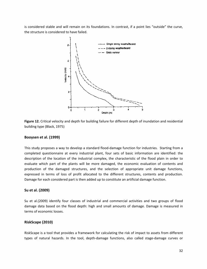
is considered stable and will remain on  its foundations.  In contrast,  if a point  lies “outside” the curve, the structure is considered to have failed.  

 

Figure 12. Critical velocity and depth for building failure for different depth of inundation and residential building type (Black, 1975)  

Booysen et al. (1999)   This study proposes a way to develop a standard flood‐damage function for industries.  Starting from a completed  questionnaire  at  every  industrial  plant,  four  sets  of  basic  information  are  identified:  the description of  the  location of  the  industrial  complex,  the  characteristic of  the  flood plain  in order  to evaluate which  part  of  the  plants will  be more  damaged,  the  economic  evaluation  of  contents  and production  of  the  damaged  structures,  and  the  selection  of  appropriate  unit  damage  functions, expressed  in  terms  of  loss  of  profit  allocated  to  the  different  structures,  contents  and  production. Damage for each considered part is then added up to constitute an artificial damage function.   

Su et al. (2009)  Su  et  al.(2009)  identify  four  classes  of  industrial  and  commercial  activities  and  two  groups  of  flood damage data based on  the  flood depth: high and  small amounts of damage. Damage  is measured  in terms of economic losses.  

RiskScape (2010)   RiskScape is a tool that provides a framework for calculating the risk of impact to assets from different types  of  natural  hazards.  In  the  tool,  depth‐damage  functions,  also  called  stage‐damage  curves  or 

  32

fragility curves, are  the most common method  to estimate potential direct damage costs. RiskScape’s fragility  curves  typically  relate  the percentage damage  (relative  to  replacement  cost)  for  a  variety of elements such as buildings, cars, household goods, relative  to  flood characteristics such as  inundation depth, velocity or duration. 

Fragility  functions  are  typically based on  either  empirical  curves developed  from historical  flood  and damage  survey  data  or  synthetic  functions  (hypothetical  curves)  based  on  expert  opinion  developed independently from specific flood and damage survey data.   Both methods have their advantages and disadvantages (Middelmann‐Fernandes, 2010). RiskScape uses a combination of both as  it has been  found  that synthetic damage curves calibrated against observed flood damage gave  the most accurate  results  (McBean et al., 1986). As damage  to buildings  typically makes  up  the most  significant  proportion  of  direct  damage  costs,  the  initial  project  focus  was  on buildings and their contents, but progress in other categories is also being made. 

Within RiskScape at present the potential to assess direct damage to lifeline infrastructure is limited to the road network and the water and wastewater system.  

USACE  (2010)  The US Army Corps of Engineers (USACE) report suggests the introduction of fragility curves in flood risk assessment.  Inspired  by  the  development  of  fragility  curves  in  seismic  events,  they  examine  what methods are used in those fields in order to identify what method could be more appropriate for flood events.  

Santella et al. (2011)   These authors propose an empirical estimation of the conditional probability of a natech event triggered by floods at chemical facilities. In this study, 10 flood events among the most severe flood disasters  in the USA  in the  last decades were analyzed. The “conditional probability of natech“  is calculated as the number  of  hazardous‐materials  releases  per  facility  exposed  to  a  flood  and  refers  to  the  probable number  of  natechs  that will  occur  in  a  specific  location  as  a  result  of  the  realization  of  the  natural disaster.  In  particular,  in  this  analysis  flood  characteristics  such  as  flood  depth were  not  taken  into account.  

Krausmann and Mushtaq (2008)  Krausmann  and  Mushtaq  (2008)  investigate  the  risk  associated  with  the  flooding  of  industrial installations and analyze qualitatively the potential impact in terms of the potential release of hazardous materials. Based on expert judgment they propose a qualitative scale  linking the flood  intensity (water depth and speed, duration) to the level of potential damage.   

  33

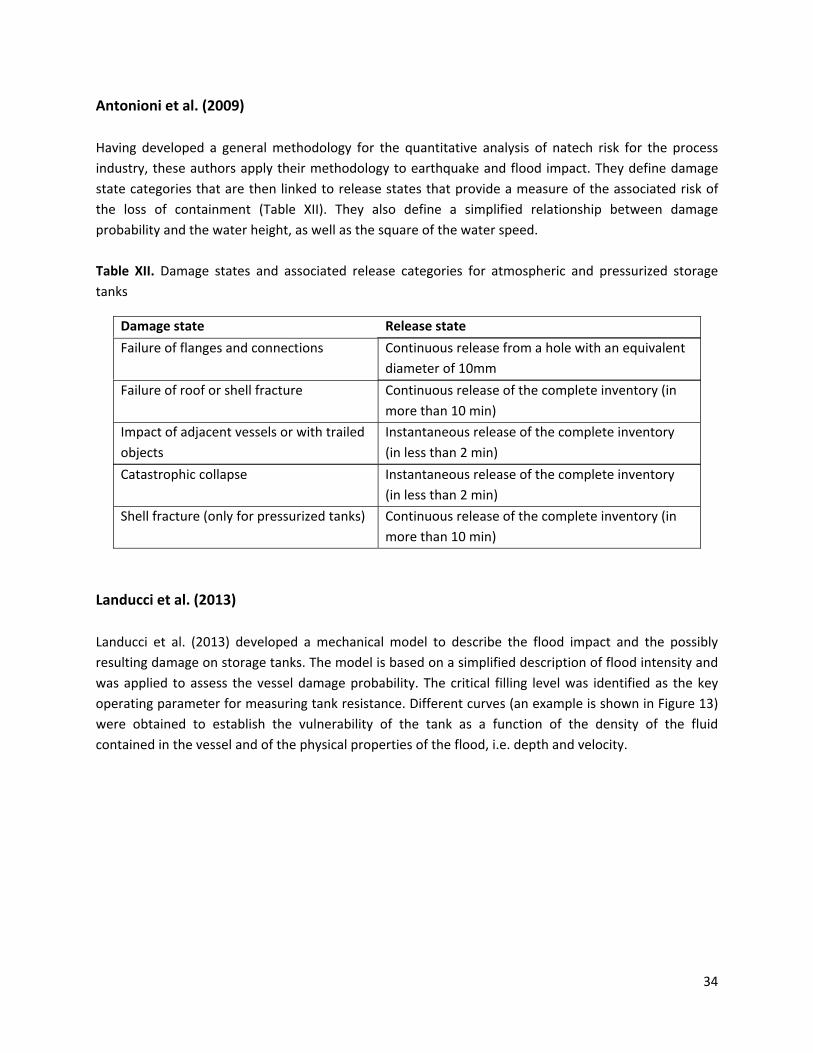
Antonioni et al. (2009)  Having developed  a  general methodology  for  the quantitative  analysis of natech  risk  for  the process industry, these authors apply their methodology to earthquake and flood  impact. They define damage state categories that are then  linked to release states that provide a measure of the associated risk of the  loss  of  containment  (Table  XII).  They  also  define  a  simplified  relationship  between  damage probability and the water height, as well as the square of the water speed.  Table  XII. Damage  states  and  associated  release  categories  for  atmospheric  and  pressurized  storage tanks 

Damage state  Release state 

Failure of flanges and connections   Continuous release from a hole with an equivalent diameter of 10mm 

Failure of roof or shell fracture  Continuous release of the complete inventory (in more than 10 min) 

Impact of adjacent vessels or with trailed objects 

Instantaneous release of the complete inventory (in less than 2 min) 

Catastrophic collapse  Instantaneous release of the complete inventory (in less than 2 min) 

Shell fracture (only for pressurized tanks)  Continuous release of the complete inventory (in more than 10 min) 

  

Landucci et al. (2013)  Landucci  et  al.  (2013)  developed  a mechanical model  to  describe  the  flood  impact  and  the  possibly resulting damage on storage tanks. The model is based on a simplified description of flood intensity and was applied  to assess  the vessel damage probability. The critical  filling  level was  identified as  the key operating parameter for measuring tank resistance. Different curves (an example is shown in Figure 13) were  obtained  to  establish  the  vulnerability  of  the  tank  as  a  function  of  the  density  of  the  fluid contained in the vessel and of the physical properties of the flood, i.e. depth and velocity. 

  34

 

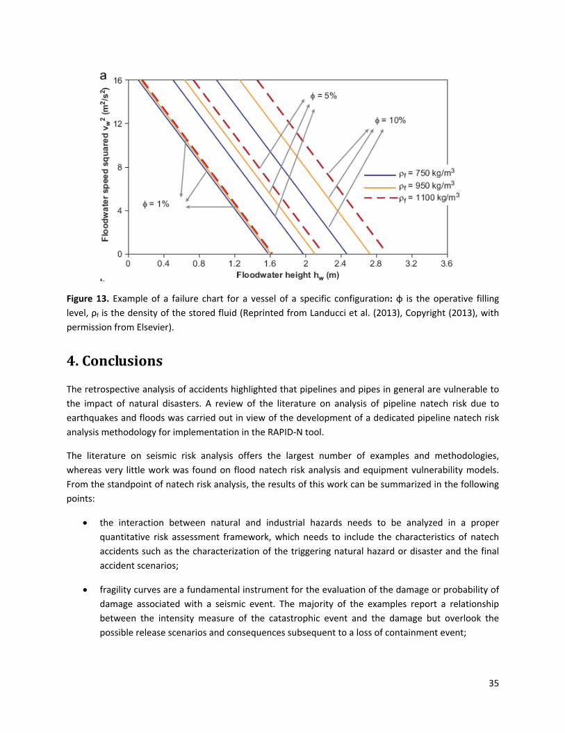
Figure 13. Example of a  failure chart  for a vessel of a  specific  configuration: φ  is  the operative  filling level, ρf is the density of the stored fluid (Reprinted from Landucci et al. (2013), Copyright (2013), with permission from Elsevier). 

4. Conclusions 

The retrospective analysis of accidents highlighted that pipelines and pipes in general are vulnerable to the  impact of natural  disasters. A  review of  the  literature on  analysis of pipeline  natech  risk due  to earthquakes and floods was carried out in view of the development of a dedicated pipeline natech risk analysis methodology for implementation in the RAPID‐N tool.  

The  literature  on  seismic  risk  analysis  offers  the  largest  number  of  examples  and  methodologies, whereas very  little work was  found on  flood natech  risk analysis and equipment vulnerability models. From the standpoint of natech risk analysis, the results of this work can be summarized in the following points: 

• the  interaction  between  natural  and  industrial  hazards  needs  to  be  analyzed  in  a  proper quantitative  risk assessment  framework, which needs  to  include  the  characteristics of natech accidents such as the characterization of the triggering natural hazard or disaster and the final accident scenarios; 

• fragility curves are a fundamental instrument for the evaluation of the damage or probability of damage  associated with  a  seismic  event.  The majority  of  the  examples  report  a  relationship between  the  intensity measure  of  the  catastrophic  event  and  the  damage  but  overlook  the possible release scenarios and consequences subsequent to a loss of containment event; 

  35

• existing studies on flood risk analysis  lack a proper characterization of damage related to flood characteristics. 

In  addition,  the  literature  review  showed  that most  studies  on  seismic  risk  concentrate  on  buried pipelines  and  ignore  above‐ground  structures.  Moreover,  the  analysis  of  past  accidents  does  not distinguish between pipelines  transporting hazardous materials and water pipelines.  In  the  latter case the  possibility  of  a  natech  event  is  not  considered.  This  empirical  data  can  be  useful  for  equipment vulnerability model  development  if  the  boundary  conditions  are  similar,  but  it  cannot  be  used  for consequence assessment. 

  36

References 

ALA, American Lifelines Alliance, Seismic fragility formulations for water systems, 2001. 

Antonioni  G.,  Bonvicini  S.,  Spadoni  G.  and  Cozzani  V.,  Development  of  a  framework  for  the  risk assessment  of  Na‐tech  accidental  events,  Reliability  Engineering  and  System  Safety,  94,  1442‐1450, 2009.

Ayala A.G. and O’Rourke M.J., Effects of the 1985 Michoacan Earthquake on water systems  in Mexico, Technical Report NCEER‐89‐0009, National Center for Earthquake Engineering Research, State University of New York, Buffalo, NY, 1989. 

Ballantyne  D.B.  and  Heubach, W.,  Earthquake  loss  estimation  for  the  city  of  Everett,  Washington, Lifelines, K/J/C 906014.00, Federal Way, Washington, 1996. 

Ballantyne D.B., Berg E., Kennedy J., Reneau R. and Wu D., Earthquake loss estimation modeling for the seattle water systems: report to US Geological Survey under Grant 14‐08‐0001‐G1526, Technical Report, Kennedy/Jenks/Chilton, Federal Way, WA, 1990. 

Barenberg  M.E.,  Correlation  of  pipeline  damage  with  ground  motions,  Journal  of  Geotechnical Engineering, ASCE, 114 (6), 706‐711, 1988. 

Black  R.D.,  Flood  proofing  rural  residences,  Report  to  the  US  Department  of  commerce,  Economic Development Administration, Washington DC, 1975. 

Booysen  H.J.,  Viljoen M.F.  and  de  Villiers  G.T., Methodology  for  the  calculation  of  industrial  flood damage and its application to industry in Vereenigng, Water SA, Vol. 25, No.1, 1999. 

Busini  V.,  Marzo  E.,  Callioni  A.  and  Rota  R.,  Definition  of  a  short‐cut  methodology  for  assessing earthquake‐related Na‐Tech risk, Journal of Hazardous Materials, 192, 329‐339, 2011. 

Campedel M., Antonioni G, Cozzani V. and Di Baldassarre G., A  framework  for  the assessment of  the industrial risk caused by floods, Safety Reliability and Risk Analysis: Theory, Methods and Applications, Martorell et al. (eds), Taylor and Francis Group,  2749‐2755, 2009. 

Campedel C., Analysis of major industrial accidents triggered by natural events reported in the principal available chemical accidents database, EUR 23391 EN, 2008. 

Campedel M., Cozzani V., Garcia‐Agreda A.  and  Salzano E., Extending  the quantitative  assessment of industrial risks to earthquake effects, Risk Analysis 28/5, 1231‐1246, 2008. 

CEN, Eurocode 8: Design of structures for earthquake resistance – Part 4: silos, tanks and pipelines, CEN European Committee for Standardization, 2006. 

  37

CCPS, Guidelines  for  chemical process quantitative  risk  analysis, 2nd  Ed., Center  for Chemical Process Safety, AIChE, New York, 2000. 

Chisolm E.I., and Matthews J.C., Impact of Hurricanes and flooding on buried infrastructure, Leadership and Management in Engineering, 12, 151‐156, 2012. 

Corigliano M, Seismic response of deep tunnels in near fault conditions, PhD, Politecnico di Torino, Italy, 2007. 

Cornell  C.A.,  Jalayer  F.,  Hamburger  R.O.  and  Foutch  D.A.,  Probabilistic  basis  for  2000/FEMA  steel moment frame guidelines, Journal of Structural Engineering, 1284, 526‐533, 2002. 

Cozzani V., Campedel M., Renni  E.  and  Krausmann  E.,  Industrial  accidents  triggered by  flood  events: analysis of past accidents, Journal of Hazardous Materials 175, 501‐509, 2010. 

Dash S.R. and Jain S.K., An overview of seismic considerations of buried pipelines, Journal of Structural Engineering, Vol. 34, No. 5, 349‐359, 2007. 

DCP, Delft Cluster Publication, Environmental impact of flooding, DC1‐233‐8, 2003. 

DeSmog Canada: http://www.desmog.ca/2013/07/03/what‐floodwaters‐mean‐alberta‐400,000‐pipelines%3F. Accessed on 22nd August 2013. 

Douglas  J.,  Ground  motion  estimation  equations  1964‐2003.  Reissue  of  ESEE  Report  No.  01‐1:  ‘A comprehensive  worldwide  summary  of  strong‐motion  attenuation  relationship  for  peak  ground accelerations and spectral ordinates (1969 to 2000)’ with correction and addictions. Research report 04‐001‐SM, Imperial College London, UK, 2004. 

Dutta D., Herath S. and Musiake K, A mathematical model for floss loss estimation, Journal of Hydrology, Vol. 227, 24‐29, 2003. 

Dziubinski M., Fratczak M. and Markowski A.S., Aspects of risk analysis associated with major failures of fuel pipelines, Journal of Loss Prevention in the Process Industries, 19, 399‐408, 2006. 

Eguchi R.T.,  Seismic  vulnerability models  for underground pipes, Proceedings of  Earthquake Behavior and Safety of Oil and Gas Storage Facilities, Buried Pipelines and Equipment, PVP‐77, ASME, New York, June, 1983. 

Eguchi R.T., Seismic hazard input for lifeline systems, Structural Safety, 10, 193‐198, 1991  

Eidinger J., Water distribution system. In: Anshel J. Schiff (ed.) The Loma Prieta, California, Earthquake of October  17,  1989  –  Lifelines.  USGS  Professional  Paper  1552‐A,  US  Government  Printing  Office, Washington, A 63‐A78, 1998. 

Eidinger J., Maison B., Lee D. and Lau B., East Bay municipal district water distribution damage  in 1989 Loma  Prieta  earthquake,  Proceeding  of  the  Fourth US  Conference  of  Lifeline  Earthquake  Engineering, ASCE, TCLEE, Monograph No.6, 240‐247, 1995. 

  38

Eidinger  J.  and  Avila  E.,  Guidelines  for  the  seismic  evaluation  and  upgrade  of  water  transmission facilities, ASCE, TCLEE, Monograph 15, 1999. 

Esposito  S.  and  Iervolino  I.,  PGA  and  PGV  spatial  correlation models  based  on  European multievent datasets, Bulletin of the Seismological Society of America, 101(5), 2532‐2541, 2011. 

Girgin  S.,  The  natech  events  during  the  17  August  1999  Kocaeli  earthquake:  aftermath  and  lessons learned, Natural Hazards and Earth System Science, Vol. 11, No. 4, 1129‐1140, 2011. 

Hamada M., Estimation of earthquake damage to lifeline system in Japan, Proceeding of the Third Japan‐US  Workshop  on  Earthquake  Resistant  Design  of  lifeline  Facilities  and  Countermeasures  for  Soil Liquefaction, San Francisco, CA, December 17‐19, 1990, Technical Report NCEER‐91‐0001, NCEER, State University of New York at Buffalo, Buffalo, NY, 5‐22, 1991. 

Honneger D.G., and Eguchi R.T., Determination of the relative vulnerabilities to seismic damage for San Diego County Water Authority: water transmission pipelines, 1992. 

Hopkins  P.,  The  structural  integrity  of  oil  and  gas  transmission  pipelines,  Comprehensive  structural integrity, Volume I, Penspen Ltd, UK, Elsevier Publishers, 2002. 

Hashash  Y.M.A.,  Schmidt  B.  and  Yao  J.I.C,  Seismic  design  and  analysis  of  underground  structures, Tunneling and Underground Technology, 16, 247‐293, 2001. 

Isoyama R.,  Ishida  E.,  Yne  K. And  Shirozu  T.,  Seismic damage  estimation procedure  for water  supply pipelines,  Twelfth  World  Conference  on  Earthquake  Engineering,  paper  no.  1762,  30  January  –  4 February, 2000, Auckland, New Zealand, 2000. 

Isoyama R. and Katayama T., Reliability evaluation of water supply system during earthquakes, Report of the institute of Industrial science, University of Tokyo, 30 (1), 1982. 

Jo  Y.  and Ahn  B.J., A method  for  the  quantitative  risk  assessment  for  transmission  pipeline  carrying natural gas, Journal of Hazardous Materials, A123, 1‐12, 2005. 

Kaplan S. and Garrick S.J., On the quantitative definition of risk, Risk Analysis, Vol. 1, No. 1, 11‐27, 1981. 

Katayama  T.,  Kubo  K.  and  Sato  N.,  Earthquake  damage  to  water  and  gas  distribution  systems, Proceedings of the  U.S. National Conference on Earthquake Engineering, EERI, Oakland, CA, 396 – 405, 1975. 

Katayama T., Kubo K. and Sato N., Quantitative analysis of  seismic damage  to buried utility pipelines, Proceedings Sixth world conference earthquake engineering institute association, New Delhi, 3369‐3375, 1977. 

Katayama  T.,  Kubo  K.  and  Sato  N.,  Earthquake  damage  to  water  and  gas  distribution  systems, Proceedings of the  U.S. National Conference on Earthquake Engineering, EERI, Oakland, CA, 396 – 405, 1975. 

  39

Krausmann E. and Baranzini D., Natech risk reduction  in the European Union, Journal of Risk Research, Vol.15, No. 8, 1027‐1047, 2012. 

Krausmann  E.,  Renni  E.,  Campedel  E.  and  Cozzani  V.,  Industrial  accidents  triggered  by  earthquakes, floods and lightning: lessons learned from a database analysis, Natural Hazards, 59, 285‐300, 2011a. 

Krausmann E., Cozzani V., Salzano E. and Renni E., Industrial accidents triggered by natural hazards: an emerging risk issue, Natural Hazards and Earth System Science, Vol. 11, No. 3, 921‐929, 2011b. 

Krausmann E. and Mushtaq F., A qualitative Natech damage scale for the  impact of floods on selected industrial facilities, Natural Hazards, 46, 179‐197, 2008. 

Landucci G., Antonioni G., Tugnoli A. And Cozzani V., Release of hazardous substances  in flood events: damage model  for atmospheric sorage  tanks, Reliability Engineering and System Safety, 106, 200‐216, 2013. 

Lanzano G., Salzano E., Santucci de Magistris F. and Fabbrocino G., Seismic vulnerability of natural gas pipelines, Reliability Engineering and System Safety, Vol. 117, 73‐80, 2013a. 

Lanzano G., Salzano E., Santucci de Magistris F. and Fabbrocino G., Seismic vulnerability of gas and liquid buried pipelines, Journal of Loss Prevention in the Process Industries, 2013b. 

Lanzano G, Salzano E, Santucci De Magistris F. and Fabbrocino G., An observational analysis of seismic vulnerability of industrial pipelines, Chemical Engineering Transaction, Vol. 26, 567‐572, 2012. 

Leville T., Shane D. and Morris J., Northridge earthquake pipeline ruptureinto the Santa Clara river, 1995 International Oil Spill Conference, Proceedings of the  IOSC  international Oil spill conference, Vol. 1995, No.1, 489 – 494, 1995. 

Mackie K. and  Stojadinivich B.,  Fragility basis  for California Highway overpass bridge  seismic decision making, PEER Report 2005/12, Pacific Earthquake Engineering Research Center, University of California, Berkley, CA, 2005.  

Mackie K. and Stojadinivich B., Seismic demand for performance‐based design of bridges, PEER Report 2003/16, Pacific Earthquake Engineering Research Center, University of California, Berkley, CA, 2003. 

Mc Bean E., Fortin M. and Gorrie  J., A critical analysis of  residential  flood damage estimation curves, Can.J.Civ.Eng.,13, 86‐94, 1986. 

Mannan S., Lees’s    loss prevention  in  the process  industries, 3rd ed. Elsevier Butterworth Heinemann, Oxford, 2005. 

Maruyama  Y.,  Yamazaki  F.,  Mizuno  K.,  Tsuchiya  Y.  and  Yogai  H.,  Fragility  curves  for  expressway embankments  based  on  damage  datasets  after  recent  earthquakes  in  Japan,  Soil  Dynamics  and Earthquake Engineering, 30, 1158‐1167, 2010. 

  40

Maruyama  Y.  and  Yamazaki  F.,  Construction  of  fragility  curve  for water  distribution  pipes  based  on damage  datasets  from  recent  earthquakes  in  Japan,  Proceeding  of  the  9th  U.S.  National  and  10th Canadian Conference on Earthquake Engineering, July 25‐29, Toronto, Ontario, Canada, Paper No. 422, 2010. 

Marzo E., Short‐cut methodologies for assessing earthquake and flood related natech risk, PhD Thesis, Politecnico di Milano, 2012. 

Mehanny  S.S.F.,  A  broad‐range  power‐law  from  scalar  based  seismic  intensity measure,  Engineering Structures, 31(7), 1354‐1368, 2009. 

Middelmann‐Fernades M.H.,  Flood  damge  estimation  beyond  stage‐damage  functions:  an  Australian example, Journal of Flood Risk Management, 3,88‐96, 2010. 

Miyajima M.  and  Hashimoto  T.,  Damage  to  water  supply  system  and  surface  rupture  due  to  fault movements  during  the  1999  JiJi  earthquake  in  Taiwan,  Proceedings  of  the  Fourth  International Conference  on  Recent  Advances  in  Geotechnical  Earthquake  Engineering  and  Soil  Dynamics  and Symposium in Honor of Professor W.D. Liam Finn, San Diego, CA, March 26‐31, 2001. 

Munich Re, http://www.munichre.com. Accessed on 22nd Nov 2013. 

NIBS, National  Institute of Building Science, Earthquake  loss estimation methodology, HAZUS technical manual, Federal Emergency Management Agency (FEMA), Washington, 2004a. 

NIBS,  National  Institute  of  Building  Science,  Flood  loss  estimation  methodology,  HAZUS  technical manual, Federal Emergency Management Agency (FEMA), Washington, 2004b. 

NTSB, National Transportation Safety Board, Evaluation of pipeline failures during flooding and   of spill response actions, San  Jacinto River near Houston, Texas, October 1994, Pipeline Special  Investigation Report, PB96‐917004, NTSB/SIR‐96/04, 1996. 

Omidvar B., Eskandari M., Peyghaleh E., seismic damage  to urban areas due  to  failed buried pipelines case  study:  fire  following  earthquake  in  the  city of  Kermanshah,  Iran, Natural Hazards,  67,  169‐192, 2013. 

O’Rourke M.J., Stewart H.E., Gowdy T.E. and Pease J.W., Lifeline and geotechnical aspects of the 1989 Loma  Prieta  earthquake,  Proceedings  of  the  Second  International  Conference  on  recent  Advances  in Geotechnical Earthquake Engineering and Soil Dynamics, St. Louis, MO., 1604‐1612, 1991. 

O’Rourke M.J., and Liu X., Response of buried pipelines subjected to earthquake effects, MCEER Monograph No.3, University of New York, Buffalo, USA, 1999. Available at: https://mceer.buffalo.edu/publications/catalog/reports/Response‐of‐Buried‐Pipelines‐Subject‐to‐Earthquake‐Effects‐MCEER‐99‐MN03.html 

O’Rourke T.D., Toprak S and Sano Y., Factors affecting water supply damage caused by the Northridge earthquake, Proceedings of the Sixth US national Conference on Earthquake Engineering, 1998. 

  41

O’Rourke M.J. and Deyoe E., Seismic damage to segment buried pipe, Earthquake Spectra, 20(4), 1167‐1183, 2004. 

O’Rourke T.D. and  Jeon  .S.S., Factors affecting  the earthquake damage of water distribution  systems, Proceedings of the Fifth US Conference on Lifeline Earthquake Engineering, Seattle, WA, ASCE, Reston, VA, 379‐388, 1999. 

O’Rourke  M.J.  and  Ayala  G.,  Pipeline  damage  due  to  wave  propagation,  Journal  of  Geotechnical Engineering, ASCE, 119 (9), 1490‐1498, 1993. 

O’Rourke T.D., Beaujon P.A. and Scawthorn C.R., Large ground deformations and their effects on lifeline facilities: 1906 San Francisco earthquake, Case  studies of  liquefaction and  lifeline performance during past earthquakes, Technical Report NCEER‐92‐0002, 2, NCEER Buffalo, NY, 1992. 

Padgett  J.E., Nielson  B.G.  and DesRoches  R.,  Selection  of  optimal  intensity measures  in  probabilistic seismic demand models of highway bridge portfolios, Earthquake Engineering & Structural Dynamics, 37(5), 711‐725, 2008.  

Parfomak  P.,  Keeping  America’s  pipelines  safe  and  secure:  key  issues  for  Congress,  CRS  Report  for Congress, R41536, 2013. 

PHMSA  advisory:  http://www.gpo.gov/fdsys/pkg/FR‐2011‐07‐27/pdf/2011‐19029.pdf.  Accessed  27th November 2013. 

Pineda‐Porras O. and Najafi M., Seismic damage for buried pipelines – challenges after three decades of progress,  Journal of Pipeline  Systems  –  Engineering  and Practice, American  Society of Civil  Engineers (ASCE), 2010. 

Pineda O. and Ordaz M., Seismic vulnerability function for high diameter buried pipelines: Mexico City’s primary water system case, International Conference on Pipeline Engineering Construction, Vol. 2, 1145‐1154, 2003. 

Pineda O. and Ordaz M., A new seismic parameter to estimate damage in buried pipelines due to seismic wave propagation, Journal of Earthquake Engineering, 11 (5), 773‐786, 2007. 

RAI2,  Small  and  Medium  Enterprises  Integrated  Flooding  Risk  Assessment  (SMEFRisk), http://www.prometeo.polimi.it/RAI/RAI_ing/RAI2_d_eng.htm, 2012. 

RAPID‐N,  Rapid  Natech  Risk  Assessment  Tool,  European  Commission,  Joint  Research  Centre, http://rapidn.jrc.ec.europa.eu, 2013. 

Renni E., Krausmann, E. and Cozzani V., Industrial accidents triggered by lightning, Journal of Hazardous Materials 184, 42‐48, 2010. 

RiskScape:  flood  fragility methodology, NIWA  Technical  Report WLG2010‐45, NIWA  Project  RSKA113, 2010. 

  42

Rossetto T. and Elnashi A., Derivation of vulnerability functions for European‐type RC structures based on observational data, Engineering Structures, 25, 1241‐1263, 2003. 

Rota R., Caragliano S., Manca D. And Brambilla S., A short cut methodology for flood‐technological risk assessment, Third  International Conference on Safety and Environment  in Process  Industry, May 11‐14, Rome, Italy, 2008. 

Rota M., Penna A. and  Strobbia C., Typological  fragility  curves  from  Italian earthquake damage data, First European Conference on Earthquake Engineering and Seismology, Geneva, Switzerland, 2006. 

Sabetta  F.,  Goretti  A.,  Luncantoni  A.,  Empirical  fragility  curves  from  damage  surveys  and  estimated strong gorund motion, 11thEuropaen Conference on Earthquake Engineering, Paris, France, 1998. 

Santella N.,  Steinberg  L.J., Aguirra G.A.,  Empirical  estimation of  the  conditional probability of natech events within the United States, Risk Analysis, Vol. 31, No. 6, 951‐968, 2011. 

Scandella  L.,  Numerical  evaluation  of  transient  ground  strains  for  the  seismic  response  analysis  of underground structures, PhD thesis, Politecnico di Milano, 2007. 

Smith D.I., Flood damage estimation – a review of urban stage‐damage curves and loss functions, Water SA, Vol. 20, No. 3, 231‐238, 1994. 

Spence  R.,  Coburn  A.W.  and  Pomonis  A,  Correlation  of  ground motion  with  building  damage :  the definition  of  a  new  damage‐based  seismic  intensity  scale,  10th  World  Conference  on  Earthquake Engineering, 551‐556, 1992. 

St John C.M. and Zahrah T.F, Aseismic design of underground structures, TUST, 2(2), 165‐197, 1987. 

Straub and Der Kiureghian,  Improved seismic  fragility modeling  from empirical data, Structural Safety, Vol. 30, 320‐336 2008. 

Su M.D., Kang  J.L. and Chang L.F.,  Industrial and commercial depth‐damage curve assessment, WSEAS Transactions on Environment and Development, Vol. 5, No. 2, 2009. 

SYNER‐G,  Systemic  seismic  vulnerability  and  risk  analysis  for  buildings,  lifeline  networks  and infrastructures safety gain, Deliverable 3.4, 2010 

Terzi V.G., Alexoudi M.N.  and Hatzigogos T.N., Numerical  assessment of damage  state of  segmented pipelines  due  to  permanent  ground  deformation,  Tenth  International  Conference  on  Applications  of Statistics and Probability in Civil Engineering, Tokyo, Japan, Paper No. 202, 2007. 

Toprak S., Earthquake effects on buried lifeline systems, PhD Thesis, Cornell University, Ithaca, NY, 1998. 

Tromans I., Behaviour of buried water supply pipelines in earthquake zones, PhD thesis, Imperial College of Science, Technology and Medicine, London, 2004.  

  43

  44

TRP,  http://www.emergency‐response‐planning.com/blog/bid/40891/Are‐the‐Floods‐of‐2011‐affecting‐Pipeline‐Safety. Accessed on 17th  October 2013. 

UPI: http://www.upi.com/Business_News/Energy‐Resources/2013/07/11/Canada‐monitoring‐pipelionlinenes‐after‐June‐floods/UPI‐22831373541807/. Accessed on 22nd August 2013. 

US Army  Corps  of  Engineers, Beyond  the  factor  of  safety:  developing  fragility  curves  to  characterize system reliability, Report ERDC‐SR‐10‐1, Washington DC, 2010. 

USGS, United States Geological Survey (USGS), http://earthquake.usgs.gov/earthquakes/shakemap/. Accessed on 20th Nov 2013. 

White  G.F.,  Choice  of  adjustment  to  floods,  Research  paper  no.  93,  University  of  Chicago,  Dept.  of Geography, 1964. 

Young  S.,  Balluz  L., Malilay  J., Natural  and  technologic  hazardous material  releases  during  and  after natural disasters: a review, Science of the Total Environment, 322, 3‐20, 2004. 

European Commission EUR 26371 EN – Joint Research Centre – Institute for the Protection and Security of the Citizen Title: Analysis of natech risks for pipelines: A review Authors: Roberta Piccinelli, Elisabeth Krausmann Luxembourg: Publications Office of the European Union 2013 – 51 pp. – 21.0 x 29.7 cm EUR – Scientific and Technical Research series – ISSN 1831-9424 ISBN 978-92-79-34813-6 doi:10.2788/42532 Abstract Natural events, such as earthquakes and floods, can trigger accidents in oil and gas pipeline with potentially severe consequences to the population and to the environment. These conjoint technological and natural disasters are termed natech accidents. The present literature review focuses on the risk analysis state-of-the-art of seismic and flood events that can impact oil and gas transmission pipelines. The research has focused on methodologies that take into account the characteristics of natech events: for instance, the characterization of the triggering natural hazard and the final accident scenarios, as well as fragility curves for the specific assessment of the potential consequences of natech accidents. The result of this research shows that the literature on seismic risk analysis offers the largest number of examples and methodologies, although most studies focused on structural damage aspects without considering the consequences of a potential loss of containment from the pipelines. Very little work was found on flood risk assessment of natech events in pipelines.

z LB-N

A-26371-EN

-N

As the Commission’s in-house science service, the Joint Research Centre’s mission is to provide EU policies with independent, evidence-based scientific and technical support throughout the whole policy cycle. Working in close cooperation with policy Directorates-General, the JRC addresses key societal challenges while stimulating innovation through developing new standards, methods and tools, and sharing and transferring its know-how to the Member States and international community. Key policy areas include: environment and climate change; energy and transport; agriculture and food security; health and consumer protection; information society and digital agenda; safety and security including nuclear; all supported through a cross-cutting and multi-disciplinary approach.