XLIII Reunión AnualNoviembre de 2008

ISSN 1852-0022ISBN 978-987-99570-6-6

Free trade agreements and the transmission of shocks across countries

Cesar CalderonIleana Jalile

ANALES | ASOCIACION ARGENTINA DE ECONOMIA POLITICA

1

Free trade agreements and the transmission of shocks across countries*

Cesar Calderona, Ileana Jalileb, *

a The World Bank, 1818 H Street NW, Washington DC 20433, USA b Universidad Nacional de Córdoba, Argentina1

Abstract

Our main goal is to evaluate the impact of free trade agreements on business cycke synchronization for a sample of 91 countries over the period 1960-2004. Our analysis involves an estimation procedure based on the features of panel data models and features of simultaneous equations models. This methodology allows us to decompose the total effect of FTA and Trade on output co-movement into their different components. Besides, we account for the possibility that the FTA itself may be endogenous and instrument for it. Our findings suggest that FTA may have two indirect channels of affecting Business Cycle Synchronization: through higher trade and inducing more symmetries in structures of production.

Resumen

El objetivo de este trabajo es evaluar el impacto que los Tratados de Libre Comercio (TLC) tiene sobre la correlación de producto entre países. Utilizamos una muestra de 91 países para el período 1960-2004 Nuestro análisis se basa en un procedimiento que tiene en cuenta característica de datos de panel y de modelos de ecuaciones simultaneas. Esta metodología nos permite descomponer en efectos directos e indirectos el efecto total del TLC y del Comercio Internacional sobre la correlación de ciclos. Además se considera la posibilidad de que los TLC sean una variable endógena en el modelo. Nuestros resultados sugieren que los TLC pueden afectar a la correlación de ciclos a través de dos canales indirectos: a través de un mayor comercio internacional e induciendo una mayor simetría en la estructura de producción de los países.

Keywords: Trade Intensity, Free Trade Agreements, Business Cycle Synchronization JEL Classification Numbers: E32, F41

* Calderón: The World Bank, Office of the Chief Economist, Latin American Region. E-mail: ccalderon@worldbank.org. Jalile: Universidad de Cordoba, Department of Economics. E-mail: ijalile@eco.unc.edu.ar. The usual disclaimer applies. The views expressed in this paper are those of the author, and do not necessarily reflect those of the World Bank and the Central Bank of Chile or their Boards of Directors. * Corresponding author. Av. Valparaiso s/n. Cdad. Universitaria. Córdoba. 5000. Argentina. Phone: +54-351-4437300 Ext. 351, Fax: +54-351-4437300

2

1.Introduction Trade integration has dramatically surged over the last 25 years and, currently, more than half of world trade is performed under actual or prospective trading blocks (Schiff, 2001). On the one hand, more than 140 regional trade agreements were in place by the end of the twentieth century, with most of them involving developing or transition economies. On the other hand, world trade has grown at a faster pace than world output in the last 25 years, thus deepening the extent of economic integration. In fact, the ratio of exports and imports to GDP of the world has increased on average from 44% in 1970 to 77% in 2005. Furthermore, countries engaging in heavier trade integration are becoming more closely linked to their macroeconomic performance, hence, the influence of important trading partners is a key factor to understand the business cycle fluctuations of national economies (Shin and Wang, 2004). There is a vast theoretical and empirical literature analyzing the channels through which business cycle fluctuations in one country are transmitted to other countries. Among the most important determinants in the literature we have: trade linkages at the inter- and intra-industry levels, demand spillovers, financial linkages, and policy coordination channels (Imbs, 2004; Baxter and Kouparitsas, 2005). Several researchers have shown that trade integration plays a crucial role in transmitting shocks across countries, thus influencing business cycle co-movements across countries �see Baxter and Kouparitsas (2005) for a review on the empirical literature. Trade linkages have been quite important in the literature of optimum currency areas: countries would benefit from sharing a common currency if they have deeper trade integration and if they have a high degree of output co-movement (Mundell, 1961; Frankel and Rose, 1997, 1998; Imbs, 1999; Rose and Engel, 2002). Theoretically, the effect of trade integration on business cycle synchronization is ambiguous. They are positively correlated: (a) if they face industry-specific shocks and trade is mostly intra-industry in nature, and (b) if business cycle fluctuations are dominated by demand shocks. Given the rising trend towards vertical specialization in world trade, developing countries have tended to become part of regional production-sharing networks and specialize in unskilled-labor-intensive stages of production (Yi, 2003). Thus, trade in parts and components of finished products has increased rapidly between developing and industrial countries (Feenstra, 1998; Deardorff, 2001).2 There is also evidence that free trade agreements may have deepened these production linkages and, hence, increased output co-movement. For instance, Chiquiar and Ramos-Francia (2005) find that, after the North American Free trade agreement (NAFTA) was enacted, the correlation between Mexican and U.S. manufacturing sectors have increased not only at the business cycle frequency but also in the long-run. They find that the rising US-Mexico co-movement after NAFTA may be explained by stronger demand linkages between the countries and deeper supply-side complementarities. In general, countries that are more engaged in �production sharing� tend to display higher business cycle synchronization (Burstein, Kurz and Tesar, 2007).3 Our main goal is to evaluate the impact of free trade agreements on business cycle synchronization for a sample of 91 countries over the period 1960-2004. Empirical research on

2 Yi (2003) shows that models of international trade with vertical specialization can explain about 70 percent of growth in world trade. 3 Burstein et al. (2007) define production sharing as trade in intermediate goods that are part of a vertically integrated production network that cross international borders. The production chain is sliced up into separate parts or stages that are undertaken in different locations according to the comparative advantage of certain regions or countries. For more details on this phenomenon see Hummels, Ishii and Yi (2001) and Yi (2003) describe this phenomenon in detail

3

the determinants of bilateral trade has primarily focused on the so-called �gravity variables,� where cross-sectional variation in the flow of trade between two countries is typically explained by cross-sectional variation in size (say, country pair�s income and population), geographic variables (distance, remoteness, border), cultural patterns (common language, colonial origin) and the presence of free trade agreements (FTA). Hence, to the extent that FTAs foster bilateral trade, there is scope for an indirect effect of FTAs on business cycle synchronization through rising trade. On the other hand, few papers have analyzed the direct effect of trade agreements on business-cycle co-movement since the signing of free trade agreements could signal further efforts for policy convergence across countries as well as treaties promoting the free flow of financial resources (say, FDI) across borders.4 This paper complements and extends the existing literature in two dimensions. First, we evaluate whether free trade agreements across countries fosters the transmission of shocks across countries. Second, we assess the direct and indirect effects of free trade agreements on business cycle synchronization by formulating a model that jointly determines the likelihood of signing free trade agreements (FTAs), the intensity of trade linkages and the degree of cycle synchronization. Here we consider the decision to sign a free trade agreement between two countries as an endogenous variable since countries may likely choose to sign FTAs for reasons that are likely to be related to the level of trade or to transmission of business cycle shocks across countries (Baier and Bergstrand, 2002, 2007 Magee, 2003). Hence, to obtain consistent estimates of the impact of FTAs on bilateral trade and on output co-movement we need to account for this endogeneity problem. In the present paper, we follow the strategy used in Baier and Bergstrand (2007) and Imbs (2004) to model the joint determination of output co-movement, trade and free trade agreements. The advantage of formulating a simultaneous equation model is that we can calculate not only the direct effect of trade agreements on output correlation but also its indirect impact through its effect on trade�which may affect the cross-country synchronization of business cycles. The rest of the paper is organized as follows: Section 2 presents the simultaneous equation model used to evaluate the impact of FTAs on cycle correlation and describes the data. Section 3 discusses the empirical evaluation on the direct and indirect effects of FTAs on business cycle synchronization, and Section 4 presents the main conclusions. 2. Methodology and Data This section discusses the modeling strategy proposed to jointly estimate the decision to sign a free trade agreement (FTA) within a country pair, the intensity of their international trade linkages and their degree of business cycle correlation. In addition, we describe the data definition and sources used in this paper. 2.1 Modeling the impact of FTAs on Business Cycle Synchronization The main goal of our paper is to estimate the impact of signing a free trade agreement (FTA) on the co-movement of output across countries. To do so, we consider a model that may account not only for the direct effects of FTAs on business cycle correlation but also the indirect effect of FTA through higher trade intensity. Note that compared to the already existing literature that measures the direct impact of deeper trade linkages on output co-movement, we account for the impact of trade intensity that may be attributed to policies of trade integration across the world.

4 For instance, Akin (2006) and Beján (2004).

4

To properly account for these effects, we use a simultaneous equation model that allows us to calculate direct and indirect effects of FTA on business cycle correlation. This strategy is not a novel one: Imbs (2004) and Garcia-Herrero and Ruiz (2007) use simultaneous-equation models to capture the impact of direct and indirect effects (through higher trade or specialization) of financial openness on business cycle synchronization. As we mentioned above, we model the decision to the sign of a trade agreement between the country pair in order to obtain consistent estimation of the effects of FTAs on cycle correlation and account for the likely problems of endogeneity and reverse causality that may arise if we fail to do so. This paper follows Baier and Bergstrand (2002), Levi-Yeyati et al. (2003) and Barro and Tenreyro (2007) in addressing this endogeneity problem. We estimate the following simultaneous-system of equations:

i,j, =

0 +

1 T

i,j, +

2 FTA

i,j, +

3 I

i,j, + u

11i,j (1)

T i,j,

= 0 +

1 FTA

i,j, +

2X

i,j, + u

2

i,j (2)

FTA i,j,

= 0 +

1 Z

i,j, (3)

where i,j indexes country pairs, ρi,j,τ denotes bilateral business cycle correlation of the country pair (i,j) over period τ, T is bilateral trade intensity in the country pair, FTA is a binary variable that takes the value of 1 if there is a free trade agreement in place within the country pair. In this simultaneous equation model, business cycles correlation, bilateral trade intensity, and free trade agreements are treated as endogenous variables, while we consider the I, X and Z matrices as exogenous variables. Note that the identification of the system requires instruments for FTA as well as differences in the set of exogenous variables of the output correlation and trade equations �that is, the I and X matrices. Business cycle synchronization. The determinants of business cycle synchronization have been extensively discussed in the literature �see Baxter and Kouparitsas (2005) for a review of the literature and Inklar, Jong-A-Pin and de Haan (2005) for a review and evaluation of determinants across OECD economies. In addition to the intensity of trade linkages (T), we include in the I matrix of business cycle correlation determinants the degree of asymmetries in structures of production for the country pair (ASP) and the intensity of intra-industry trade (GLI) �with α3 y α4 denoting their corresponding coefficients to estimate. The coefficient α1 in the business cycle correlation equation captures the direct effect of trade intensity on output co-movement. The theoretical sign of this coefficient is ambiguous: it depends on the nature of the shocks driving business cycles and whether the pattern of trade between countries is intra- or inter-industry. We expect α1 to be positive if business cycles are driven by strong demand spillovers and/or patterns of intra-industry trade dominate within the country pair. The direct effect of free trade agreements on output correlation is captured by the coefficient α2. We expect α2 to be positive with free trade agreements deepening the production links between countries in a world with vertical specialization5 and/or FTAs leading to other types of policy convergence across countries. Indeed several authors have noted that one of the major benefits

5 Lowering the trading costs due to a Free Trade Agreement might lead to greater specialization. Specialization can take place within a given sector (Vertical specialization) or between sectors. To the extent that shocks are sector-specific and common to all countries, the first type of specialization will lead to more co-movement of shocks

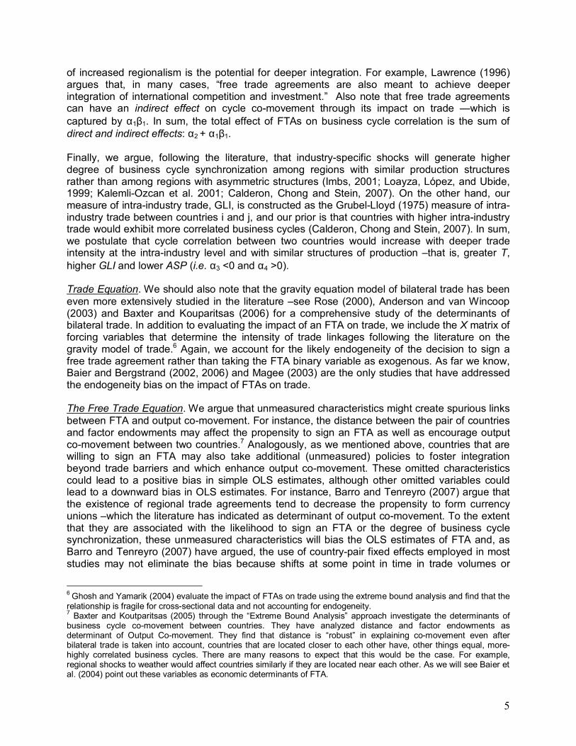
5

of increased regionalism is the potential for deeper integration. For example, Lawrence (1996) argues that, in many cases, �free trade agreements are also meant to achieve deeper integration of international competition and investment.� Also note that free trade agreements can have an indirect effect on cycle co-movement through its impact on trade �which is captured by α1β1. In sum, the total effect of FTAs on business cycle correlation is the sum of direct and indirect effects: α2 + α1β1. Finally, we argue, following the literature, that industry-specific shocks will generate higher degree of business cycle synchronization among regions with similar production structures rather than among regions with asymmetric structures (Imbs, 2001; Loayza, López, and Ubide, 1999; Kalemli-Ozcan et al. 2001; Calderon, Chong and Stein, 2007). On the other hand, our measure of intra-industry trade, GLI, is constructed as the Grubel-Lloyd (1975) measure of intra-industry trade between countries i and j, and our prior is that countries with higher intra-industry trade would exhibit more correlated business cycles (Calderon, Chong and Stein, 2007). In sum, we postulate that cycle correlation between two countries would increase with deeper trade intensity at the intra-industry level and with similar structures of production �that is, greater T, higher GLI and lower ASP (i.e. α3 <0 and α4 >0). Trade Equation. We should also note that the gravity equation model of bilateral trade has been even more extensively studied in the literature �see Rose (2000), Anderson and van Wincoop (2003) and Baxter and Kouparitsas (2006) for a comprehensive study of the determinants of bilateral trade. In addition to evaluating the impact of an FTA on trade, we include the X matrix of forcing variables that determine the intensity of trade linkages following the literature on the gravity model of trade.6 Again, we account for the likely endogeneity of the decision to sign a free trade agreement rather than taking the FTA binary variable as exogenous. As far we know, Baier and Bergstrand (2002, 2006) and Magee (2003) are the only studies that have addressed the endogeneity bias on the impact of FTAs on trade. The Free Trade Equation. We argue that unmeasured characteristics might create spurious links between FTA and output co-movement. For instance, the distance between the pair of countries and factor endowments may affect the propensity to sign an FTA as well as encourage output co-movement between two countries.7 Analogously, as we mentioned above, countries that are willing to sign an FTA may also take additional (unmeasured) policies to foster integration beyond trade barriers and which enhance output co-movement. These omitted characteristics could lead to a positive bias in simple OLS estimates, although other omitted variables could lead to a downward bias in OLS estimates. For instance, Barro and Tenreyro (2007) argue that the existence of regional trade agreements tend to decrease the propensity to form currency unions �which the literature has indicated as determinant of output co-movement. To the extent that they are associated with the likelihood to sign an FTA or the degree of business cycle synchronization, these unmeasured characteristics will bias the OLS estimates of FTA and, as Barro and Tenreyro (2007) have argued, the use of country-pair fixed effects employed in most studies may not eliminate the bias because shifts at some point in time in trade volumes or

6 Ghosh and Yamarik (2004) evaluate the impact of FTAs on trade using the extreme bound analysis and find that the relationship is fragile for cross-sectional data and not accounting for endogeneity. 7 Baxter and Koutparitsas (2005) through the �Extreme Bound Analysis� approach investigate the determinants of business cycle co-movement between countries. They have analyzed distance and factor endowments as determinant of Output Co-movement. They find that distance is �robust� in explaining co-movement even after bilateral trade is taken into account, countries that are located closer to each other have, other things equal, more-highly correlated business cycles. There are many reasons to expect that this would be the case. For example, regional shocks to weather would affect countries similarly if they are located near each other. As we will see Baier et al. (2004) point out these variables as economic determinants of FTA.

6

output co-movement may be related to a change in the propensity to form an FTA. As we can observe, standard omitted variable problems arise in the estimation of the effect of trade agreement on the extent of co-movement of shocks, and it is necessary to instrument for it to obtain consistent estimation of the coefficients in the system. 2.2 On the estimation technique Baier and Bergstrand (2002, 2007) have found that the bias induced by omitted variables is the major source of endogeneity facing the estimation of FTA effects on gravity equations.8 To address this endogeneity problem in a cross-section study they used an efficient two step IV estimator (2SIV) suggested by White (1984). This procedure delivers the asymptotically efficient estimator among the class of IV estimators, even in the presence of a non-spherical variance covariance matrix (VCV) for the error term in the structural equation.9 For their cross-section analysis, they conclude using a wide (though not an exhaustive) array of feasible instrumental variables for FTA, that IV estimation is not a reliable method for addressing the endogeneity bias of trade agreement in the gravity equation. On the other hand, they argue that one can draw strong and reliable inferences about the effects of trade agreements using the gravity equation applied to panel data. On the other hand, Magee (2003) follows Trefler (1993) and points to simultaneity biases as the major source of potential endogeneity of FTA and he uses the simultaneous equations approach with a 2SLS estimation to address this issue. However, as noted in Baier and Bergstrand (2002, 2006) and shown in Heckman (1978) and Maddala (1983, p.118), the system of equations estimated in Magee is not logically consistent. In order to address the endogeneity problem of the FTA dummy variable we use the two step IV estimator (2SIV) suggested by White (1984) applied to our panel dataset. This methodology requires finding instruments for the choice of signing a free trade agreement and implementing a two-stage procedure. In the first step, we run a probit model of the FTA dummies on all the exogenous variables included in the model, plus some additional exogenous controls (instruments). As instruments for FTA, Z, we use a set of variables that the literature indicates as variables who could affect the probability of sign a Free Trade Agreement between a pair of countries but which are not correlated with unobservable for the econometrician in the equations of the system. In the second stage, this methodology implies to use the predicted probabilities of FTA, predicted P(FTA), as instruments for FTA in the equations of the system. Barro and Tenreyro (2007), following a similar approach, use an IV variable for Currency Unions in trade and co-movement regressions for their panel dataset.10 The advantage of using this methodology to address the endogeneity problem on our panel dataset over using country-pair fixed effects is, as argued in Barro et al. (2007), that the use of country-pair fixed effects employed in most studies may not eliminate the bias because shifts at

8 The authors argue that two countries tend to have an FTA based on a list of factors which includes the same factors that tend to explain large trade flows. They asked how is the unobserved heterogeneity in trade flows determinants associated with the likelihood of an FTA. They suggest that FTA and the error term in the gravity equation are negatively correlated, and the FTA coefficient will tend to be underestimated. 9 Baier and Bergstrand apply this class of IV estimator using the Average Treatment Effect methodology. Levy-Yeyati and Sturzenegger (2003), on the other hand, apply this class of IV estimator in order to estimate the impact of exchange rate regimes (dummy variable) on economic growth. They consider the possibility of reverse causation and use this technique to address the endogeneity problem. 10 Barro and Tenreyro (2007) use the likelihood that two countries independently adopt the currency of the same anchor country as an instrument for whether they share or not a common currency.

7

some point in time in trade volumes or output co-movement may be related to a change in the propensity to form an FTA. In summary, our analysis involves an estimation procedure based on the features of panel data models and features of simultaneous equations models. This methodology allows us to decompose the total effect of FTA and Trade on output co-movement into their different components. Besides, in addition to the business synchronization and the trade equation we account for the possibility that the FTA itself may be endogenous and instrument for it with a set of exogenous variables in the system. As in Baier and Bergstrand (2002, 2006), Levy-Yeyati et al. (2003) and Barro et al. (2007) we follow the 2SIV methodology in order to address the endogeneity problem of the FTA dummy variable. We use a panel of pair of countries across time, so each equation can be formulated for each time periods, with parameters constrained to be equal across time-periods. We follow Wacziarg and Tavares (2001) model, where each relationship formulated for each time period is equivalent to a panel data model where the data for each country pair have been stacked over time. As in Wacziarg et al. (2001), if we stack the errors for each equation and country pair into a vector εij , we are able to formulate the usual assumptions on the error vector, namely:

E( i)= 0 and E( ij, ij´)= The off-diagonal elements of Σ are the error covariances across time and across structural relationships, which are unconstrained. Stacking the error terms over all observations leads to a block diagonal covariance matrix Σ. The assumption that the reduced form error term can co-vary across time for a single relationship is tantamount to allowing the error term to contain a country pair specific effect that is independent from right hand side variables, an approach equivalent to the random effects model. Given the above, important additional restrictions imposed on the covariance matrix of the full disturbance error term stem from the assumption that Σ does not depend on the country pair subscript ij . This rules out heteroskedasticity and spatial autocorrelation11. Using equation-by-equation instrumental variables estimation on the structural form model would yield consistent estimates, but efficiency will be not attained because cross-equation disturbance correlations are neglected. In order to impose cross-period parameter equality restrictions and to exploit efficiency gains from the correlations of error terms for each structural relationship across time, one could use a variant of single equation IV whereby each structural relationship is estimated for all time periods jointly using three stage least squares as in Barro (1996). This method takes into account cross-period correlations but does not exploit the information inherent in the fact that error terms may not be independent across structural relationships. We estimate the full set of equations jointly using 3SLS. This is an IV-GLS estimator which achieves consistency through instrumentation and efficiency through appropriate weighting. In summary, in our first approximation we are going to follow the 3SLS methodology and for instrumenting FTA we are going to follow the Levy-Yeyati et al. (2003), Bair and Bergstrand (2002, 2007) and Barro and Tenreyro (2007) works. Finally we are going to estimate the full set of equations using 2SIV equation by equation to provide a further check on the robustness of the estimation. To support the claim that FTA is endogenous we are going to estimate the equations using OLS and the compare this with our methodologies proposed.

11 However we report standard errors that are robust to heteroskedasticity.

8

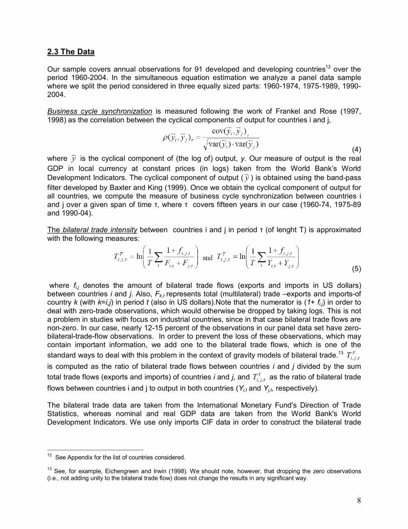
2.3 The Data Our sample covers annual observations for 91 developed and developing countries12 over the period 1960-2004. In the simultaneous equation estimation we analyze a panel data sample where we split the period considered in three equally sized parts: 1960-1974, 1975-1989, 1990-2004. Business cycle synchronization is measured following the work of Frankel and Rose (1997, 1998) as the correlation between the cyclical components of output for countries i and j,

(4) where y~ is the cyclical component of (the log of) output, y. Our measure of output is the real GDP in local currency at constant prices (in logs) taken from the World Bank�s World Development Indicators. The cyclical component of output ( y~ ) is obtained using the band-pass filter developed by Baxter and King (1999). Once we obtain the cyclical component of output for all countries, we compute the measure of business cycle synchronization between countries i and j over a given span of time τ, where τ covers fifteen years in our case (1960-74, 1975-89 and 1990-04). The bilateral trade intensity between countries i and j in period τ (of lenght T) is approximated with the following measures:

(5) where fi,j denotes the amount of bilateral trade flows (exports and imports in US dollars) between countries i and j. Also, Fk,t represents total (multilateral) trade �exports and imports-of country k (with k=i,j) in period t (also in US dollars).Note that the numerator is (1+ fi,j) in order to deal with zero-trade observations, which would otherwise be dropped by taking logs. This is not a problem in studies with focus on industrial countries, since in that case bilateral trade flows are non-zero. In our case, nearly 12-15 percent of the observations in our panel data set have zero-bilateral-trade-flow observations. In order to prevent the loss of these observations, which may contain important information, we add one to the bilateral trade flows, which is one of the standard ways to deal with this problem in the context of gravity models of bilateral trade.13 F

jiT τ,, is computed as the ratio of bilateral trade flows between countries i and j divided by the sum total trade flows (exports and imports) of countries i and j, and Y

jiT τ,, as the ratio of bilateral trade flows between countries i and j to output in both countries (Yi,t and Yj,t, respectively). The bilateral trade data are taken from the International Monetary Fund's Direction of Trade Statistics, whereas nominal and real GDP data are taken from the World Bank's World Development Indicators. We use only imports CIF data in order to construct the bilateral trade

12 See Appendix for the list of countries considered. 13 See, for example, Eichengreen and Irwin (1998). We should note, however, that dropping the zero observations (i.e., not adding unity to the bilateral trade flow) does not change the results in any significant way.

9

measures.14 Following Feenstra (2005) we prefer to use the importers� reports, whenever they are available, given that these are more accurate than reports by the exporter.15 Next, we compute averages over the annual data for the non-overlapping 15-year periods spanning 1960-2004. Our discussion of the results will mainly focus on the bilateral trade figures normalized by output since it captures with more accuracy the effective degree of integration between two countries.16 Free trade agreements. The FTA dummy variable was constructed using the FTAs notified to the GATT/WTO under GATT Articles XXVI or the Enabling Clause for developing countries.17 This source is compatible and updates the data used in Levy-Yeyaty, Stein and Daude (2002), Lawrence (1996) and Frankel (1997. We use annual data of the FTA dummy variable to obtain the predicted FTA variable which will be used as the instrumental variable in the simultaneous equations system, as we explained above. As we consider three fifteen-years period in our system of equation, the FTA dummy variable in the Cycle Synchronization and Trade equations would be equal to one in each period if the country pair have signed an FTA in any of the first 5 years of each period, such estimation tries to take into account the typical phase-in period of almost all FTAs.18 Intra-industry trade between countries i and j is computed as the Grubel-Lloyd (1975) measure of intra-industry trade between countries i and j, GLIi,j:

( )∑∑

+

−−=

k

kji

kji

k

kji

kji

ji mx

mxGLI

,,

,,

, 1 (6)

where kjix , and k

jim , are exports from country i to country j and imports from country i to country j, respectively, and k represents an index over industries. Our measure of intra-industry trade between countries i and j, GLIi,j, represents the proportion of intra-industry trade in the total trade of these two countries. Our data on intra-industry trade has been obtained from the NBER-U.N. World Trade data as collected by Feenstra (2005). We use here the SITC (Rev. 2) two-digit level bilateral exports and imports between countries i and j. Finally we compute the corresponding 15-year period averages over this annual dataset. For a more detailed description of the data, see Feenstra (2005). Similarities in the structure of production. Evidence shows that industry-specific shocks will generate higher degree of business cycle synchronization among regions with similar production structures rather than among regions with asymmetric structures (Imbs, 2001; Loayza, López, and Ubide, 1999; Kalemli-Ozcan et al. 2001; Imbs, 2003). This variable is approximated using

14 Although there was data for imports FOB on the IMF�s Direction of Trade Statistics, the data availability was more limited. That is, it represents at most 20 percent of the coverage with imports CIF. 15 A problem which is typical of bilateral trade data is export flows from country i to country j are not necessarily equal to import flows of country j from country i. 16 For example, the share of bilateral trade to total trade between countries i and j could be very high (say, for a pair of remote countries). However, both could have a small external sector and, therefore, the share of bilateral trade to their outputs could be very small. 17 See http://www.wto.org/english/tratop_e/region_e/summary_.xls 18 As Bair and Bergstrand (2007) indicate virtually every FTA is �phase-in� typically over 10 years.It is reasonable to expect that an FTA entered �legally� in 1975 to not come into economic effect fully until 1985. Thus, in order to assess the entire economic effect of an FTA, we measure the impact on Cycle Correlation and Trade of an FTA signed in any of the first 5 years of each fifteen years-period, so the estimated coefficient associated to FTA can measure the entire economic effect on Trade and BC of and FTA.

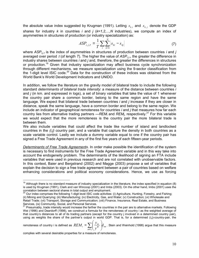
10

the absolute value index suggested by Krugman (1991). Letting iks , and jks , denote the GDP shares for industry k in countries i and j (k=1,2,...,N industries), we compute an index of asymmetries in structures of production (or industry specialization) as:

∑∑=

−=t

N

kkjkiji ss

TASP

1,,

1τ (7)

where ASPi,j,τ is the index of asymmetries in structures of production between countries i and j averaged over period τ (of length T). The higher the value of ASPi,j,τ, the greater the difference in industry shares between countries i and j and, therefore, the greater the differences in structures or production.19 Given that industry specialization may affect business cycle synchronization through different mechanisms, we measure specialization using the 9-sector classification from the 1-digit level ISIC code.20 Data for the construction of these indices was obtained from the World Bank�s World Development Indicators and UNIDO. In addition, we follow the literature on the gravity model of bilateral trade to include the following standard determinants of bilateral trade intensity: a measure of the distance between countries i and j (in km. and expressed in logs), a set of binary variables that take the value of 1 whenever the country pair share a common border, belong to the same region and have the same language. We expect that bilateral trade between countries i and j increase if they are closer in distance, speak the same language, have a common border and belong to the same region. We include an indicator of geographical remoteness for countries i and j that measures how far each country lies from alternative trading partners �REMi and REMj, respectively.21 For this variable we would expect that the more remoteness is the country pair the more bilateral trade is between them. We also include variables that could affect the trade like number of island and landlocked countries in the (i,j) country pair, and a variable that capture the density in both countries as a scale variable control. Lastly we include a dummy variable equal to one if the country pair has signed a Free Trade Agreement in any of the first five years of each fifteen-year periods. Determinants of Free Trade Agreements. In order make possible the identification of the system is necessary to find instruments for the Free Trade Agreement variable and in this way take into account the endogeneity problem. The determinants of the likelihood of signing an FTA include variables that were used in previous research and are not correlated with unobservable factors. In this context, Baier and Bergstrand (2002) and Magge (2003) propose a set of variables that explain the decision to sign a free trade agreement between a pair of countries based on welfare enhancing considerations and political economy considerations. Hence, we use as forcing

19 Although there is no standard measure of industry specialization in the literature, the index specified in equation (8) is used by Krugman (1991), Clark and van Wincoop (2001) and Imbs (2003). On the other hand, Imbs (2001) uses the correlation between sectoral shares in total output and employment. 20 Our index comprises the following 1-digit level ISIC code activities: (i) Agriculture, Hunting, Forestry, and Fishing; (ii) Mining and Quarrying; (iii) Manufacturing; (iv) Electricity, Gas, and Water; (v) Construction; (vi) Wholesale and Retail Trade; (vii) Transport, Storage and Communication; (viii) Finance, Insurance, Real Estate, and Business Services, (ix) Community, Social, and Personal Services. 21 Presumably, trade intensity would increase the farther the countries in the pair are to alternative markets. Following Wei (1996) and Deardorff (1998), we construct a formula for the remoteness of country i as the weighted average of that country�s distances to all of its trading partners (except for the country j involved in a determined country pair), using as weights the share of the partner�s output in world GDP. That is, for a determined (i,j)-country-pair, the

remoteness of country i is defined as imjm

Wm

i dyy

REM ∑≠

= . Stein and Weinhold (1998) argue that this measure

complies with several desirable properties for a measure of remoteness.

11

variables for the decision to sign free trade agreements: the distance between countries (in logs), the real GDPs, differences in the capital labor ratio in the country pair and a measure of country risk of each member of the country pair, which tries to assess the �cost� of bilateral trade policy negotiations. We expect that the net gain from an FTA between two countries increase if the countries are closer in distance (Baier and Bergstrand, 2004), and we used the information on country location to measure the Great Circle distance �our proxy to measure distance between countries i and j. (Rose and Engel, 2002). On the other hand, we expect that the net welfare gain from FTAs increases the larger is the economic size of the countries involved (Baier and Bergstrand, 2002). Intuitively, the welfare gains from FTAs should be higher for countries with larger absolute factor endowments (and, consequently, larger real GDPs).22 Real GDPs are taken from the World Penn Tables and are in 1996 PPP dollars. A more direct measure of endowments is constructed using data for capital stocks taken from Fajnzylber et al. (2005) and expressed in 1987 US dollars (in logs). Differences in capital-labor ratios are used to assess whether a wider difference in relative factor endowment would enhance the benefits of an FTA between a country pair. In Heckscher-Ohlin type models of trade, ceteris paribus the transportation and/or transaction costs, the benefits of an FTA would be maximized whenever a pair of countries displays a wider dispersion in relative factor endowments so that comparative advantage is fully exploited. Relative factor endowment differences are measured as the absolute value of the difference in (the logs of the) capital-labor endowment ratio of countries i and j23. On the other hand, Magee (2003) and Levy (1997) follow a political economy argument to suggest that preferential trade deals are more likely to be supported if the countries are on the same side of the world median capital-labor ratio. The smallest the difference between capital-labor ratios, the more likely two countries are to sign an FTA. Finally, we expect that the (i,j) country pair is more unlikely to sign a free trade agreements if at least one of the countries is unable to conduct sustainable economic policies. For instance, if one country has unstable exchange rate policies or decides unilaterally to raise tariffs or impose restrictions to their exports, we could expect that other countries would be less likely to sign a preferential trade agreement or a free trade agreement with the unstable government in that country. In short, the lower the costs of bilateral trade negotiations, the more likely the countries with sign an FTA. These costs will be lower in countries with less regulatory intrusion by the governments and the more credible are the governments in committing to policies. Here we use the sub-index investment profile from the ICRG political risk index published by the PRS group. Investment profile evaluates factors affecting the risk to investment that are not covered by other political, economic and financial risk components. This measure takes values from 0 to 12, with

22 The formation of an FTA between two (economically) large partners create trade in more varieties than an FTA between two small partners, improving utility more in large countries relative to small ones. Thus, larger exporter and importer real GDPs should be associated with a higher likelihood of an FTA. 23 As Baier and Bergstrand (2004) indicate, we have to consider that the decision between two countries to have an FTA or not in t depends upon economic characteristics in t. However, income and factor endowments vary over time and have likely been influenced by trade liberalization. For example, an FTA in place between two countries in the third period (1989-2004) could have been formed well before 1989. Since an FTA formed several years prior to 1989 likely influenced subsequent trade and cycle correlation- which then influenced economic growth- income and capital stocks in this period may well be endogenous. To account for this, we tried two alternative specifications for the FTA equation. First, we used the data for 1960 on incomes and capital and labor stocks from the data set mentioned above. Second, for the pair of countries who signed an FTA in t we used the value for gdp and K/L ratio in this year (Date of Entry into Force) for the subsequent years, this allow us to consider that the decision to form an FTA took into account economic characteristics in t, and the reverse causality possibility. Both specifications did not present any significant differences from the result using current annual data for these two variables.

12

higher values indicating higher levels of governance, and comprises three categories: contract viability / expropriation, profits repatriation, and payment delays. We have constructed a variable which measures the absolute value of the difference of this sub-index (in logs) between countries i and j.

3. Empirical Assessment This section present the evidence on the effects of free trade agreements on cycle synchronization using our simultaneous equation model for a panel data of country-pairs based on 15-year average information of 91 countries over the period 1960-2005. We first discuss the partial correlation between the variables of interest in our analysis using least squares (OLS) estimates. Second, we tackle the issue of endogeneity equation by equation using two-stage instrumental variable techniques (2SIV), where we address the issue of endogeneity of the decision of signing a free trade agreement. Finally, we jointly estimate the system specified in equations (1) through (3) using three-stage least squares (3SLS), which accounts not only for likely endogeneity of explanatory variables but also efficiency in the estimation of the standard errors. 3.1 Pooled estimation Table 1 reports equation-by-equation pooled estimation of each equation of the system. The results presented in the first three columns of results are based on the measure of bilateral trade intensity normalized by output ( Y

jiT τ,, ), while the last three columns of results the estimates based

on the measure of bilateral trade intensity normalized by total trade ( FjiT τ,, ). We have to

remember that in the co-movement equations, the sample consists of one observation for each fifteen-year period on each country pair. So, all the endogenous variables in our system, the regresors and the IVs (in the next sub-section) are the averages over each period. As we can observe there are no significant differences between the point estimation using either of the two measures of trade �normalized by trade or output. However, the discussion of the results will mainly focus on the bilateral trade figures normalized by output since it captures with more accuracy the effective degree of integration. Also, note that the business cycle synchronization and bilateral trade equations include period-dummies (for the period 1975-1989 and 1990-2004) so that we control for specific shocks to each period (i.e. global shocks) which have affected to all country pairs. In addition to that, we have added country pair dummies to this specification in order to capture the differences in output correlation and bilateral trade between each country pair group. In this paper, we have defined binary variables corresponding to: (a) country pairs of industrial countries, (b) mixed industry and developing country pairs, and (c) country pairs of developing countries. On average, we have found that mixed industrial-developing and developing-country-pairs have weaker output synchronization and lower trade intensity compared to industrial-country�pairs.24

24 This results are available from the authors upon request.

13

Table 1: OLS Estimation

(1) Output CorrelationGLI 0.43458 *** 0.39446 *** 0.42633 *** 0.393239 ***

0.045 0.05418 0.04566 0.054553ASP -0.06644 *** -0.0738 *** -0.05438 *** -0.08091 ***

0.016 0.02005 0.01717 0.020371FTA 0.07462 *** 0.076436 ***

0.02588 0.025793Trade 0.00749 *** 0.00594 *** 0.0060 *** 0.00761 *** 0.00558 *** 0.005509 ***

0.0009 0.001 0.0017 0.00094 0.0013 0.001765Period-Specific DummiesCountry-Pair DummiesAdj R-squaredNumber of obs

(2) Trade Equationfta 0.44671 *** 0.461769 **

0.15468 0.159531lndistjk -1.1093 *** -0.80631 *** -0.59591 *** -0.9545 *** -0.64732 *** -0.51052 ***

0.0571 0.056 0.05042 0.05641 0.05539 0.052099remote 7.67768 *** 5.3567 *** 5.39928 *** 7.57886 *** 5.65371 *** 5.709661 ***

0.3598 0.349 0.30671 0.35949 0.3483 0.316849bderjk 1.40037 *** 1.52485 *** 1.41674 *** 1.68667 *** 1.89361 *** 1.708041 ***

0.2251 0.212 0.18621 0.22156 0.2109 0.190341comlang 0.90643 *** 0.72064 *** 0.28183 *** 0.936 *** 0.76109 *** 0.371846 ***

0.0938 0.089 0.07686 0.09409 0.08881 0.079943comreg 1.19901 *** 1.39682 *** 1.61424 *** 1.22447 *** 1.47024 *** 1.757246 ***

0.1296 0.131 0.12165 0.1284 0.13034 0.125516n_landl -1.7801 *** -1.41136 *** -1.36336 *** -1.8358 *** -1.55767 *** -1.49925 ***

0.0733 0.076 0.07015 0.07271 0.07661 0.074585n_isle -0.1412 ** -0.62258 *** -0.54482 *** -0.4309 *** -0.73 *** -0.54383 ***

0.0638 0.065 0.05792 0.06387 0.0641 0.059513lnDensityj 0.31135 *** 0.26172 *** 0.25457 *** 0.216019 ***

0.025 0.02248 0.02516 0.023037lnDensityk 0.22161 *** 0.17179 *** 0.2068 *** 0.155526 ***

0.022 0.02006 0.02232 0.020671Period-Specific DummiesCountry-Pair DummiesAdj R-squaredNumber of obs 7393 739310170 7664 7664 9498

Yes Yes0.3349 0.359 0.3597 0.3337 0.3395 0.34

(ii) (iii)Normalized by TradeNormalized by Product

(i) (ii) (iii) (i)Coef. Coef. Coef. Coef.Coef.

0.0449 0.0641 0.0649 0.0461 0.0623

Yes

0.06327664 7664 9498 7393 739310170

YesYes

Yes YesYes Yes

Yes YesYes Yes Yes

Yes Yes Yes Yes

Coef.

Yes YesYes Yes Yes Yes

Normalized by Product(i) (ii) (iii)

Normalized by Trade(i) (ii) (iii)

Note: Numbers in italics bellow the estimated coefficients represent standard errors. Intercepts and dummies are not reported. ***Significant at 1%, **Significant at 5%, *Significant at 10%

14

Business cycle synchronization. An examination of our output correlation regression equation shows that bilateral trade has a significant effect regardless of the measure of bilateral trade intensity used and the specification presented in Table 1. The point estimate of our bivariate regression �column (i)� suggests that a one standard deviation increase in the coefficient of bilateral trade intensity is associated with an increase in output correlation from an initial mean of 0.074 to 0.102 when bilateral trade is normalized by output.25 Our second specification �column (ii)� adds to our basic specification the degree of output specialization, ASP, and a measure of intra-industry trade, GLI. Finally, our specification in column (iii) includes the binary variable of free trade agreements, FTA. Again, FTA takes the value of 1 whenever the country pair has a free trade agreement in force in any of the first five years of each period (and 0 otherwise). Our estimates from Table 1 show that country pairs with higher output co-movement tend to show: (a) higher bilateral trade linkages, (b) higher degrees of intra-industry trade, (c) similar patterns of specialization, and (d) they are likely to have a free trade agreement in place. Using the coefficient estimates in column (iii) of Table 1, we find that the presence of an FTA between a country pair is related to higher output correlation by 0.074626. However, these results should be taken with caution. Why? First, the regression explains a very small fraction of the variability of the output co-movement. Second, the likely endogeneity of bilateral trade and FTA may lead to biased and inconsistent coefficient estimates. Bilateral Trade Equation. Our estimates for the gravity model of bilateral trade are consistent with the literature and all the explanatory variables have the expected sign. That is, a country pair (i,j) tend to display a higher degree of bilateral trade intensity if the countries are larger in size (as proxied by population density), closer in distance, remote from the rest of the world, share a common border, speak the same language, belong to the same region, and are neither landlocked countries nor island countries. Regarding our variable of interest, we find that the coefficient of free trade agreement (FTA) is positive and statistically significant regardless of the measure of our dependent variable. This implies that countries with an FTA in place usually tend to trade more. However, we have to remark that we fail to account here for the likely endogeneity of signing free trade agreements. 3.2 Addressing endogeneity issues: Equation by equation Our main goal of this paper is to accurately identify the impact of FTAs on cycle correlation and that implies evaluating the endogenous decision for any country pair or group of countries to sign free trade agreements. In addition, as the literature vastly shows, trade linkages and cycle correlation can be endogenously determined so that we need to instruments to identify the impact of trade on cycle correlation (see Rose and Engel, 2002; Imbs, 2004; Calderon, Chong and Stein, 2007). Following our discussion in Section 2, we estimate a probit equation for the likelihood of a country pair in having a free trade agreement in place using an annual data set of variables that

25 This result is obtained by multiplying the coefficient estimate and the standard deviation of bilateral trade intensity measure. In the case of the coefficient of bilateral trade normalized by output, we have that the increase in output correlation is equal to 0.074 + 0.0075*3.893= 0.103. This result is close to the estimates in Calderón, Chong and Stein (2007). 26 As we mentioned above, we use the FTA dummy variable equal to one in each period considered if the pair of countries signed an FTA in any of the first 5 years of each fifteen-year period. This allows us to account into account the phase in period in almost every FTA and in this way we can to take into account the total economic impact of an FTA on cycle and trade equations.

15

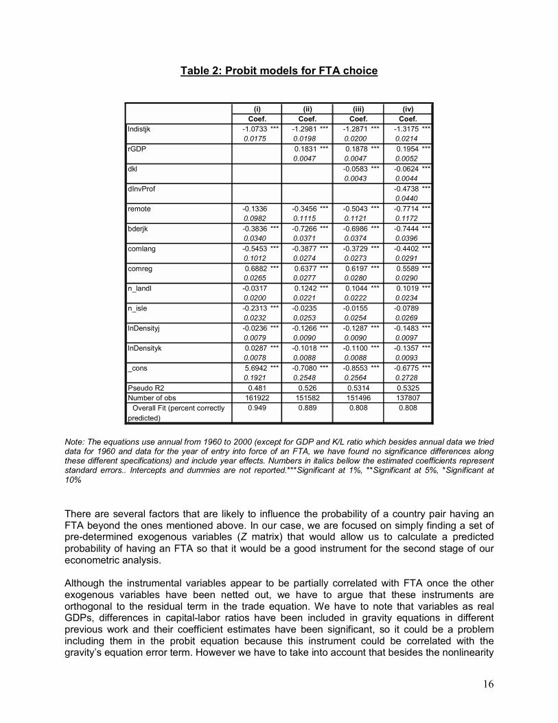
were identified in previous empirical research. Table 2 reports the results of probit equation, used to generate the predicted P(FTA) .The specification in column (i) of Table 2 shows the regression estimation where predicted probabilities of having an FTA are obtained just using exogenous variables in the system and no variables are included in Z. Wooldridge (2002) suggests that, although feasible, one can �rarely justify� this procedure for one reason: the predicted probability �which is then used as instrument in the second stage� and the exogenous variables of the system are typically highly correlated. The following specifications have added different variables in Z where the identification of the equation of the system arises from the nonlinearity of the probit function and the instruments in Z. In column (ii) of Table 2, we add the real GDPs in order to test the hypothesis that the net welfare gains from an FTA between a pair of countries increases the larger their economic sizes are. Furthermore, column (iii) of Table 2 tests the hypothesis that the probability of having an FTA is higher the larger the difference between two countries relative factor endowments �after accounting for the economic sizes of the country pair27. Finally, column (iv) in Table 2 adds the explanatory variable that captures the costs of bilateral trade policy-negotiations. The coefficient estimates in Table 2 show that many of the economic determinants of signing an FTA have the expected sign and are consistent with the existing literature. First, we find that greater distance between two countries lowers the probability of having an FTA. Second, the coefficient of (geographical) remoteness is negative and statistically significant indicating that the net welfare gains from an FTA for trading partners increases as their remoteness from the rest of the world increases. Third, the variables included in Z have coefficient estimates consistent with the theoretical model and are statistically significant. That is, two countries are more likely to have an FTA in place, the larger their economies are (in size) and the lower are their costs of bilateral trade policy-negotiations. Finally, the larger the difference between capital-labor ratios across the country-pair, the lower the probability of signing an FTA �which is consistent with the findings of Magee (2003) and Levy (1997). In order to check the goodness of fit of our estimations we present two alternative measures of the probit regression: the pseudo-R2 and the percentage of correctly predicted FTAs. For all specifications, the pseudo-R2 is larger than 0.5. On the other hand, the percentage of times that P(FTA) matches FTA (which equals 1 is an FTA exists, and 0 otherwise) is approximately 96 percent �that is, the existence of FTAs is correctly predicted in most of the cases in all specifications.28

27 As we mentioned above, in order to estimate the predicted(FTA) variable we used annual data for dependent and independent variables. For the case of GDPs and K/L ratios, besides using annual data, we have tried two other different specifications to account for reverse causality possibility: data for 1960 and data for year of entry into force countries pair that signed an FTA on incomes and capital labor stocks. All the possibilities provided similar results (this results are available from the authors upon request). 28 Usually the threshold is set to 0.5, however because of the fact that there are more observations where no FTA were observed than observations with an effective FTA we could evaluate the goodness of fit of the models for its ability to predict the observations with no FTA. In order to do that we can impose a lower threshold at the level 0.35 (in order to set a more stringent condition for the model to prove its quality) and the estimated models predict correctly about 95 percent of the cases.

16

Table 2: Probit models for FTA choice

lndistjk -1.0733 *** -1.2981 *** -1.2871 *** -1.3175 ***0.0175 0.0198 0.0200 0.0214

rGDP 0.1831 *** 0.1878 *** 0.1954 ***0.0047 0.0047 0.0052

dkl -0.0583 *** -0.0624 ***0.0043 0.0044

dInvProf -0.4738 ***0.0440

remote -0.1336 -0.3456 *** -0.5043 *** -0.7714 ***0.0982 0.1115 0.1121 0.1172

bderjk -0.3836 *** -0.7266 *** -0.6986 *** -0.7444 ***0.0340 0.0371 0.0374 0.0396

comlang -0.5453 *** -0.3877 *** -0.3729 *** -0.4402 ***0.1012 0.0274 0.0273 0.0291

comreg 0.6882 *** 0.6377 *** 0.6197 *** 0.5589 ***0.0265 0.0277 0.0280 0.0290

n_landl -0.0317 0.1242 *** 0.1044 *** 0.1019 ***0.0200 0.0221 0.0222 0.0234

n_isle -0.2313 *** -0.0235 -0.0155 -0.07890.0232 0.0253 0.0254 0.0269

lnDensityj -0.0236 *** -0.1266 *** -0.1287 *** -0.1483 ***0.0079 0.0090 0.0090 0.0097

lnDensityk 0.0287 *** -0.1018 *** -0.1100 *** -0.1357 ***0.0078 0.0088 0.0088 0.0093

_cons 5.6942 *** -0.7080 *** -0.8553 *** -0.6775 ***0.1921 0.2548 0.2564 0.2728

Pseudo R2Number of obs

Overall Fit (percent correctly predicted)

1378070.808

Coef.(ii) (iii) (iv)

Coef. Coef. Coef.(i)

0.808

0.4811619220.949

0.5261515820.889

0.5314 0.5325151496

Note: The equations use annual from 1960 to 2000 (except for GDP and K/L ratio which besides annual data we tried data for 1960 and data for the year of entry into force of an FTA, we have found no significance differences along these different specifications) and include year effects. Numbers in italics bellow the estimated coefficients represent standard errors.. Intercepts and dummies are not reported.***Significant at 1%, **Significant at 5%, *Significant at 10% There are several factors that are likely to influence the probability of a country pair having an FTA beyond the ones mentioned above. In our case, we are focused on simply finding a set of pre-determined exogenous variables (Z matrix) that would allow us to calculate a predicted probability of having an FTA so that it would be a good instrument for the second stage of our econometric analysis.

Although the instrumental variables appear to be partially correlated with FTA once the other exogenous variables have been netted out, we have to argue that these instruments are orthogonal to the residual term in the trade equation. We have to note that variables as real GDPs, differences in capital-labor ratios have been included in gravity equations in different previous work and their coefficient estimates have been significant, so it could be a problem including them in the probit equation because this instrument could be correlated with the gravity�s equation error term. However we have to take into account that besides the nonlinearity

17

of the probit function to provide the �identification� of the gravity equation, we tried different specifications for the instruments in this specification dated for the first year of our sample, 1960 and for the Date of Entry into Force of the FTA. While this can never be known, we suppose that these variables are not correlated with their own average for each of the three periods considered or any other unobservable in the trade equation. In all the model specifications that follows we have used our Probit last specification to construct the Predicted(FTA) variable which will then be used as instrument in the second stage of this procedure. Before analyzing the 3SLS estimation of the system we present the results of the system estimation using equation by equation estimation procedures29. First, we used the 2SLS technique to estimate the system of equations. . Column (i) of Table 3 presents the results of the 2SLS procedure. If all equations are correctly specified, system procedures are asymptotically more efficient than a single-equation procedure such as 2SLS. But single-equation methods are more robust. If one equation in the system is misspecified, the 3SLS estimates of all parameters are generally inconsistent. Our estimates for the 2SLS show that a pair of countries with higher cycle synchronization tend to show: (a) higher bilateral trade linkages, (b) higher degree of intra-industry trade, (c) similar patterns of specialization. The coefficient related to FTA in output co-movement equation (α2) although positive is not statistically different from zero. Concerning to the trade equation, we obtained the expected sign and significance from the different gravity variables- however, the coefficient associated to FTA in this equation (β1) is statistically different from zero at 10% of significance- . Second, we have estimated only the Business Cycle Correlation Equation with IVs (using appropriate instruments for Trade and FTA30.) Column (ii) of Table 3 presents the results. Although coefficients changes compared to the OLS specification (iii) � normalized by Output- of Table 1, it is important to notice that FTA becomes statistically insignificant. The IV estimation, however, stills pools together the direct and indirect effects of FTA over Output Correlation and we have to take into account that if indirect effects through trade channel are statistically significant � it means, if FTA affects trade- there is a place for an impact of FTA on cycle correlation. 3.3 Addressing endogeneity issues: Joint estimation of the model The 3SLS estimations of our simultaneous equation model are presented in columns (iii) and (iv) of Table 3. This Table reports the results of the 3SLS estimation that accounts not only for the endogeneity of output co-movement, trade intensity and free trade agreements, but also for an efficient estimation of the standard errors. As we can observe in column (iii), the coefficient associated to trade in the business cycle synchronization equation (α1) is higher relative to the one estimated using least squares.31 In this 29 As we mentioned above, in the co-movement equations, the sample consists of one observation for each period. So, in the different estimation procedures we use the averages over each period of the regresors and the IVs. 30 The IV for FTA is built from the probit equation model (iv) in Table 2. As instruments for Trade we use the gravity variables shown in the trade equation. 31 As in Frankel and Romer (1998) and Calderón et al (2007) instrumenting trade with gravity variables results in higher point estimates, since it controls for possible omitted variables or simultaneity bias which can cause that the coefficient tend to be underestimated.

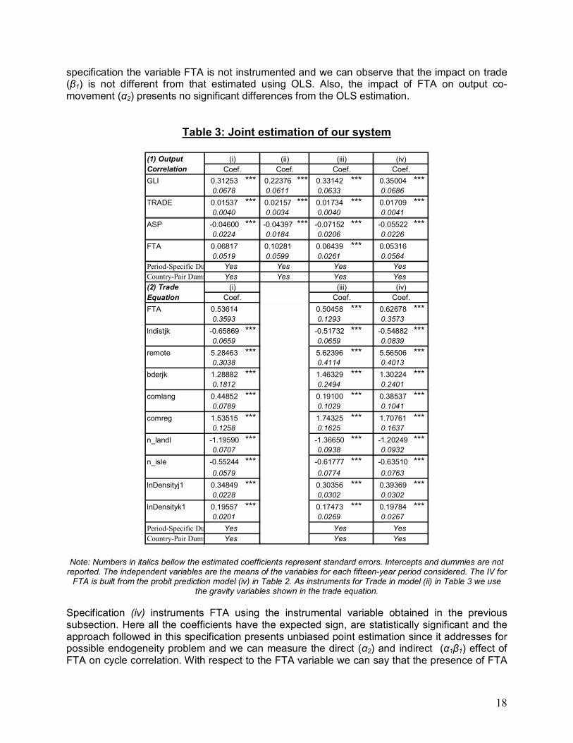
18

specification the variable FTA is not instrumented and we can observe that the impact on trade (β1) is not different from that estimated using OLS. Also, the impact of FTA on output co-movement (α2) presents no significant differences from the OLS estimation.

Table 3: Joint estimation of our system

(1) Output CorrelationGLI 0.31253 *** 0.22376 *** 0.33142 *** 0.35004 ***

0.0678 0.0611 0.0633 0.0686TRADE 0.01537 *** 0.02157 *** 0.01734 *** 0.01709 ***

0.0040 0.0034 0.0040 0.0041ASP -0.04600 *** -0.04397 *** -0.07152 *** -0.05522 ***

0.0224 0.0184 0.0206 0.0226FTA 0.06817 0.10281 0.06439 *** 0.05316

0.0519 0.0599 0.0261 0.0564Period-Specific DuCountry-Pair Dumm(2) Trade EquationFTA 0.53614 0.50458 *** 0.62678 ***

0.3593 0.1293 0.3573lndistjk -0.65869 *** -0.51732 *** -0.54882 ***

0.0659 0.0659 0.0839remote 5.28463 *** 5.62396 *** 5.56506 ***

0.3038 0.4114 0.4013bderjk 1.28882 *** 1.46329 *** 1.30224 ***

0.1812 0.2494 0.2401comlang 0.44852 *** 0.19100 *** 0.38537 ***

0.0789 0.1029 0.1041comreg 1.53515 *** 1.74325 *** 1.70761 ***

0.1258 0.1625 0.1637n_landl -1.19590 *** -1.36650 *** -1.20249 ***

0.0707 0.0938 0.0932n_isle -0.55244 *** -0.61777 *** -0.63510 ***

0.0579 0.0774 0.0763lnDensityj1 0.34849 *** 0.30356 *** 0.39369 ***

0.0228 0.0302 0.0302lnDensityk1 0.19557 *** 0.17473 *** 0.19784 ***

0.0201 0.0269 0.0267Period-Specific DuCountry-Pair Dumm

Yes Yes

(iii)Coef.

(iv)Coef.

Yes Yes

Yes

Coef. Coef.(iii) (iv)

Yes Yes

Yes Yes

(i)Coef. Coef.

Yes

Yes

(ii)

Yes

Coef.(i)

Yes Yes

Note: Numbers in italics bellow the estimated coefficients represent standard errors. Intercepts and dummies are not reported. The independent variables are the means of the variables for each fifteen-year period considered. The IV for

FTA is built from the probit prediction model (iv) in Table 2. As instruments for Trade in model (ii) in Table 3 we use the gravity variables shown in the trade equation.

Specification (iv) instruments FTA using the instrumental variable obtained in the previous subsection. Here all the coefficients have the expected sign, are statistically significant and the approach followed in this specification presents unbiased point estimation since it addresses for possible endogeneity problem and we can measure the direct (α2) and indirect (α1β1) effect of FTA on cycle correlation. With respect to the FTA variable we can say that the presence of FTA

19

implies on average higher cycle correlation with respect the country pair that has not signed a trade agreement, however this results is not statistically significant. The coefficient of ASP (α4) is negative and statistically significant and our result suggests that country pairs with similar structures of production (i.e. similar patterns of specialization) have higher business cycle synchronization. Note that this result is robust to the specification used. Finally, we find that countries with higher degree of intra-industry trade tend to show larger cyclical output correlation in all specifications. In addition we have found that the coefficient that measures the impact of FTA on the gravity equation (β1) is equal to 0.63, it means that the impact of a free trade agreement is to (almost) double trade between country pairs (e0.61=1.88 or 88 percent increase)32 . However, using the OLS methodology the estimated impact of an FTA (β1) is to increased bilateral trade in 53 percent approximately. Hence we can observe that not accounting for endogeneity of FTAs can attenuate the impact of a trade agreement in the volume of bilateral trade, just as suggested by the theoretical papers mentioned above. Finally, we have found that the gravity variables shown the expected sign and all are statistically significant: shorter distance, common language, common border, common region, higher density, remoteness, landlocked area and number of isles in the country pair increase bilateral trade between them. In sum, our 3SLS estimation of the system indicates that if we do not take into account endogeneity problem of variables as FTA and Trade in the econometric estimation, we can underestimate their impact on flows of bilateral trade and cycle correlation respectively. Besides, if we only estimate the Cycle Correlation equation with the appropriate instruments for FTA and Trade �as presented in column (ii)- we could say that FTA have no impact at all on Business Cycle Synchronization. However, 3SLS system estimation shows that there is place for an indirect impact of FTA on Output Co-movement via trade and with these results we can assess the direct and indirect channels through which Bilateral Trade and FTA impact on Business Synchronization Besides, as a measure of robustness of our results we can observe that there are not significant differences between the point estimations from 2SLS and 3SLS so this is evidence that our 3SLS is done properly. Lastly, we have to note that there are drawbacks from employing fixed-effects estimation in our context, mainly because of many of the exogenous variables used in our previous estimation are not time varying and therefore can not be used either as instruments or as control variables in a fixed-effects procedure. Besides of that, our methodological strategy was to control for every possible variable which is constant across time and it could be associated with FTA in the gravity equation. 3.4 Measuring the impact of FTAs on Cycle Correlation As we have mentioned above there is place for an indirect impact of FTA on Output Co-movement via trade and with our 3SLS estimation we can now assess the direct and indirect channels through which Bilateral Trade and FTA can impact on Business Synchronization, and 32 Baier and Bergstrand using a panel data set for 96 countries for the period 1960-2000 found that a FTA increase bilateral trade of 97 percent, which is closer to our results.

20

test their statistical significance. In order to do that we have to take into account the estimated coefficients of our system of equations by 3SLS � column (iv) of Table 3- , and we can obtain and measure the direct and indirect channels through which Trade and Free Trade Agreements affects Business Cycle Synchronization. According to our system of equations specification - see Section 2.3- the direct effect of trade, captured in α1, is either the reflection of commerce due to the sign of a free trade agreement (α1β1) or standard geographical Trade (α1β2). So, separate estimates of β1 and β2 make it possible to identify the proportion of α1, that comes from FTA and which from geographical issues33. The direct effect of FTA on co-movement is captured in α2 while its indirect effect comes via trade (α1β1). In order to test the statistical significance of indirect and indirect channels the standard errors on the products of coefficients are calculated by a linear approximation around the estimated parameter values using the formula for the variance of linear function of random variables to calculate the corresponding standard errors Using our 3SLS estimation we can calculate the values of these direct and indirect effects. In Table 4 we present these values and the main results are as follows: First, we find that about two-thirds of the direct effect of trade on cycle correlation (α1) can be attributed to geographical trade and the remaining one-third to trade agreements. Finally the direct effect of FTA on output co-movement is not statistically different from cero, so it suggests that there are no direct effects of FTA on output co-movement and that impact of FTA on synchronization comes only via enhanced trade linkages.

Table 4: Measuring the direct and indirect effects

Total Effect of Trade on Business Synchronization Direct Fta trade α1β1= 0.012679 (2.39)

Geographic Trade α1β2=0.0098832 (3.59)

Total Effect of FTA on Business Synchronization Direct Indirect FTA α2= 0.053 (0.056)

Via Trade α1β1= 0.012679 (2.39)

Note: Numbers in parenthesis represent the t-statistics based on our efficiently estimated standard errors. 3.5 - Extensions to the Simultaneous Equation Model

33 As in Imbs (2004) the value of β2 were obtained using the 3SLS fitted values for trade on gravity variables.

21

In this subsection we present a first approximation to a possible extension of our benchmark empirical model. We consider the possibility of an additional channel, and report estimates pertaining to the determinants of Business Cycle Correlation. As we mentioned above, the effect of trade integration on business cycle synchronization is ambiguous. If trade integration implies more intra-industry trade between a country pair and they face industry-specific shocks we would expect a higher output co-movement. Given the rising trend toward vertical specialization - Hummels, Ishii and Yi (2001) argue that production sharing accounts for more than one-third of world export growth between 1970 and 1995- and its consequent increase in intra-industry trade we would expect, again, a higher output co-movement between the countries engaged in this regional production-sharing networks. The purpose of this subsection is to examine if trade integration � the presence of an FTA- could enhance this kind vertical specialization. There is evidence that FTA may have deepened these production linkages, for example Chiquiar y Ramos Francia (2005) find that, after the NAFTA was enacted, demand linkages between the countries and supply-side complementarities increased. On the other hand, Burstein, Kurz and Tessar (2007) argue that countries that are more engaged in production sharing exhibit higher bilateral manufacturing output correlations. They develop a quantitative model of international business cycles that generates a positive link between the extent of vertically integrated production-sharing trade and internationally synchronized business cycles. In sum, in this subsection we try to identify a new channel through which an FTA can have an impact of Business Cycle Synchronization. We consider the following system of equations to be estimated: ρi,j,τ = α0 + α1 T i,j,τ + α2 FTA i,j,τ + α3 ASP i,j,τ + α4 GLI i,j,τ + u11i,j T i,j,τ = β0 + β1 FTA i,j,τ + β2X i,j,τ + β3ASP i,j,τ + u2 i,j ASP i,j,τ = γ0 + γ1 GapY i,j,τ+ γ2 FTA i,j,τ + u3 i,j FTA i,j,τ = δ0 + δ 1 Z i,j,τ In this new specification of our system of equations we have added the variable that measures the similarities in the structure of production between the pair of countries i and j (ASP) in the Trade equation in order to capture the idea that similarities in the production structure may affect the nature of the impact of trade integration on cycle correlation, the coefficient associated to ASP (α3) captures the extent to which bilateral trade can be accounted for by the similarities in the two countries´ economic structures, that is on the basis of intra-industry trade. Besides, we have added a new equation to the system, namely, the equation where the index of similarities in the production structure is the endogenous variable. As determinants of specialization we have included the FTA variable in order to capture the idea that openness to goods trade results in specialization. Most classical models make this prediction. For instance, falling transport cost in Dornbusch, Fischer and Samuelson (1977) result in a narrowing nontraded sector, as it becomes cheaper to import goods rather than produce them domestically. Thus resources are free up and used more intensely in fewer activities. Standard trade theory (Heckscher-Ohlin paradigm) predicts that openness to trade would lead to an increasing specialization in production along industry lines, and inter-industry patterns of international trade (as typically

22

observed among developing countries). We also have used as control for the equation of similarity of production the pair wise difference of per capita GDPs based on Imbs and Wacziarg (2003) and Imbs (2004). The gap between their GDPs try to measure the different stages of development of the pair of countries considered. 3SLS estimation of the system is presented in Table 5 and shows that the coefficient associated with ASP in the Equation of Trade is negative and statistically significant indicating that countries with similar economic structures trade more, a quantification of the extent of intra-industry trade. We have to note that once we control for ASP in the Trade Equation, the effect of FTA vanishes. Probably this mean that in previous specifications the FTA variable was capturing the idea that we have mentioned above, FTA could lead to more specialization � vertical specialization in this case-. Precisely, in our last equation we analyze this idea and we have found that trade integration �it means the sign of a FTA between the pair of countries- on average increases the similarity of production between the pair of countries. We also have found that countries at different stages of development have significantly higher ASP, that is, tend to display different economic structures.

Table 5: Joint estimation of our new system

GLI 0.3703 *** fta1 -0.3813 0.1 difyppp1 6.45E-06 ***0.065 0.216 0

TRADE 0.0141 *** lndistjk -0.7581 *** FTA -0.1649 ***0.004 0.083 0.018

ASP -0.2224 *** remote 7.0455 ***0.036 0.423

FTA -0.0082 bderjk 1.3614 ***0.034 0.244

comlang 0.3732 ***0.106

comreg 1.1767 ***0.171

n_landl -1.0479 ***0.093

n_isle -0.6739 ***0.076

lnDensityj1 0.3558 ***0.031

lnDensityk1 0.1827 ***0.027

ASP -2.8305 ***0.315

(2) Trade Equation (3) ASP Equation(1) Output Correlation

Note: Numbers in italics bellow the estimated coefficients represent standard errors. Intercepts and dummies are not reported. Include Period and Country Pair Dummies. The independent variables are the means of the variables for each fifteen-year period considered. The IV for FTA is built from the probit prediction model (iv) in Table 2. In this specification of the system the effect of FTA on cycle synchronization is only indirect through the impact on the similarity in productive structures of the pair of countries and is positive and equal to ( γ2*β3*α2 ). This implies that trade integration tend to make more similar the productive structures (vertical specialization) of the country pair which explain intra-industry trade.

23

4.- Conclusions In this paper we have attempted to assess the role of FTA in Business Cycle Synchronization and Trade by estimating a joint system of equations using the 3SLS methodology. There are different benefits from this approach. First, it allows us to identify and quantify the channels through which FTA affect output co-movement. Second, this methodology provides us an IV-GLS estimator which achieves consistency through appropriate instrumentation and efficiency through appropriate weighting. In our empirical assessment we used a panel data for 91 developed and developing countries over the period 1960-2004. While there are likely endogeneity problems associated with trade intensity and FTA as explanatory variables for output synchronization, in theory one could eliminate those biases using the appropriate set of instruments. However as we mentioned above the coefficients estimated through this methodology will give us the net effects of this variables on output co-movement and probably the impact of one variable - trade in our case- on synchronization could be reinforced for the indirect effect of other explanatory variable- FTA in our case-. In order to analyze the direct and indirect effect of FTA we have applied the 3SLS methodology. From our regression analysis, we find that FTA have no direct impact on business cycle correlation but it has a significant indirect impact on output correlation through higher trade. In fact, our results suggest that about two-thirds of the impact of trade on output co-movement can be attributed to geographical trade and the remaining one-third to free trade agreement. In other words, the system estimation points out that the model without the FTA variable in the equation of trade only should seek to reproduce two-third of the value of α1 when the country pair has an FTA in force, or that if a pair of countries has an FTA then the impact of trade on output co-movement would be increased in the amount α1β1 . Finally, we have presented a first approximation to a possible extension of our system of equations. This new system tries to measure the links between trade integration and intra-industry trade and its impact on Output Correlation. Previous empirical research has shown that there is a trend towards vertical specialization in world trade, besides there is also evidence that FTA may have deepened these production linkages and, hence, increased output co-movement. We have found that the effect of FTA on cycle synchronization is only indirect through the impact on the similarity in productive structures of the pair of countries and is positive and equal to ( γ2*β3*α2 ). This implies that trade integration tend to make more similar the productive structures (vertical specialization) of the country pair which explain intra-industry trade. In sum, we have found that FTA may have 2 indirect channels of affecting Business Cycle Synchronization: through higher trade and inducing more symmetries in structures of production. Only through the 3SLS methodology used we can disentangle direct and indirect effects on business cycle synchronization. Reduced form equation of Output Co-movement could give us misleading information on the impact of FTAs on cycle correlation.

24

References Akin, Cigdem, 2006. �Multiple Determinants of Business Cycle Synchronization.� George

Washington University, manuscript Anderson, James E. and Eric van Wincoop, 2003. �Gravity with Gravitas: A Solution to the

Border Puzzle.� American Economic Review 93(1), 170-192 Baier, Scott L., and Jeffrey H. Bergstrand, 2007. �Do free trade agreements actually increase

members' international trade?" Journal of International Economics 71(1), 72-95 Baier, Scott L., and Jeffrey H. Bergstrand, 2004. �Economic determinants of free trade

agreements," Journal of International Economics 64(1), 29-63 Baier, Scott L., and Jeffrey H. Bergstrand, 2002. �On the Endogeneity of International Trade

Flows and Free Trade Agreements,� manuscript Barro, Robert J., 1996. �Democracy and growth,� Journal of Economic Growth 1 (1). Barro, Robert J and Silvana Tenreyro, 2007. "Economic Effects Of Currency Unions," Economic

Inquiry, Western Economic Association International, vol. 45(1), pages 1-23, 01. Baxter, Marianne, 1995. �International Trade and Business Cycles. In: Grossman, G., and K.S.

Rogoff, Eds., Handbook of International Economics, Vol. 3. Amsterdam: North-Holland. Baxter, Marianne and Robert G. King, 1999. �Measuring Business Cycles: Approximate Band-

Pass Filters for Economic Time Series.� The Review of Economics and Statistics 81, 575-593

Baxter, Marianne and Michael A. Kouparitsas, 2005. �Determinants of business cycle co-movement: a robust analysis,� Journal of Monetary Economics 52(1), 113-157

Baxter, Marianne and Michael A. Kouparitsas, 2006. �What determines bilateral trade flows?� NBER Working Paper 12188, May

Bejan, Maria, 2006. Some Business Cycles Consequences of Signing Trade Agreements: The Case of NAFTA. EUI-RSCAS Working Papers Series 03 (2007): pp. 1-27.

Burstein, Ariel, Christopher Kurz, and Linda Tesar, 2007. �Trade, production sharing and the international transmission of business cycles.� Journal of Monetary Economics, forthcoming.

Calderón, César, Alberto Chong, and Ernesto Stein, 2007. �Trade Intensity and Business Cycle Synchronization: Are Developing Countries any Different?� Journal of International Economics 71, 2-21

Calderón, César, Norman Loayza amd Pablo Fajnzylber. 2005. �Economic Growth in Latin America and the Caribbean: Stylized Facts, Explanations, and Forecasts�. The World Bank Publications.

Canova, Fabio, and Harris Dellas, 1993. �Trade Interdependence and the International Business Cycle,� Journal of International Economics 34, 23-47

Chiquiar, Daniel and Manuel Ramos-Francia, 2005. �Trade and business cycle synchronization� evidence from Mexican and U.S. manufacturing industries,� North American Journal of Economics and Finance 16, 187-216

Clark, T.E., and Eric van Wincoop, 2001. �Borders and Business Cycles,� Journal of International Economics 55, 59-85

Deardorff, A.V., 2001. �Fragmentation in simple trade models,� North American Journal of Economics and Finance 12(2), 121-137

Feenstra, R., 1998. �Integration of trade and disintegration of production in the global economy,� The Journal of Economic Perspectives 12(4), 31-50

Finger, J.M., and M.E. Kreinin, 1979. �A Measure of Export Similarity and its possible uses,� The Economic Journal 89, 905-912

25

Frankel, Jeffrey A., and Andrew K. Rose, 1998. �The endogeneity of the optimum currency area criteria,� The Economic Journal 108, 1009-1025

Garcia-Herrero, Alicia and Juan M. Ruiz, 2007. �How Much do Trade and Financial Linkages Affect Business Cycle Syncronization for Small Open Economies?� Bank of Spain, manuscript

Ghosh, Sucharita, and Steven Yamarik. 2004a. �Does trade creation measures up? A reexamination of the effects of regional trade agreements,� Economics Letters 82, 213-219

Ghosh, Sucharita, and Steven Yamarik. 2004b. �Are regional trade arrangements trade-creating? An application of extreme bounds analysis,� Journal of International Economics 63(2), 369-395

Hummels, David L., Jun Ishii, and Kei-Mu Yi, 2001. �The Nature and Growth of Vertical Specialization in World Trade.� Journal of International Economics 54(1), 75-96.

Imbs, Jean, 2001. �Co-Fluctuations,� CEPR Discussion Paper 2267, October Imbs, Jean, 2004. �Trade, Finance, Specialization, and Synchronization,� The Review of

Economics and Statistics 86, 723-734 Inklar, Robert, Richard Jong-A-Pin, and Jakob de Haan, 2005. �Trade and business cycle

synchronization in OECD countries: A re-examination.� CESifo Working Paper 1546, September

Levy Yeyati, Eduardo, and Federico Sturzenegger, 2003. �To Float or to Fix: Evidence on the Impact of Exchange Rate Regimes,� American Economic Review 93(4), 1173-1193.

Loayza, Norman, Humberto Lopez, and Angel Ubide, 2001. �Co-movements and sectoral Dependence: Evidence for Latin America, East Asia, and Europe. IMF Staff Papers 48, 367-396

Kalemli-Ozcan, S., Bent E. Sorensen, and Oved Yosha, 2001. �Economic Integration, Industrial Specialization, and the Asymmetry of Macroeconomic Fluctuations,� Journal of International Economics 55, 107-137

Kouparitsas, Michael A., 2001. �Evidence of the North-South Business Cycle,� Federal Reserve Bank of Chicago, Economic Perspectives, First Quarter, 46-59

Magee, Christopher S., 2003. �Endogenous Preferential Trade Agreements: An Empirical Analysis," Contributions to Economic Analysis & Policy, Vol. 2, Issue 1, Article 15. Available at: http://www.bepress.com/bejeap/contributions/vol2/iss1/art15

Mundell, Robert, 1961. �A Theory of Optimum Currency Areas,� American Economic Review 51, 509-517

Rose, Andrew K., 2000. �One Money, One Market: The Effect of Common Currencies on Trade.� Economic Policy Volume 16, Issue 33, 9-45

Rose, Andrew K., and Charles Engel, 2002. �Currency Unions and International Integration,� Journal of Money, Credit, and Banking 34(3), 804-825

Schiff, Maurice, 2001. �Chile�s Trade Policy: An Assessment.� Central Bank of Chile Working Paper 151, April

Shin, Kwanho, and Yunjong Wang, 2004. �Trade integration and business cycle synchronization in East Asia,� Asian Economic Papers 2(3), 1-20

Tavares, José and Romain Wacziarg, 2001. �How Democracy Affects Growth,� European Economic Review 45(8), 1341-1379

Santos Silva, J.M.C., and Silvana Tenreyro, 2006. �The Log of Gravity Trade.� The Review of Economics and Statistics 88(4), 641-658

Yi, K-M., 2003. Can Vertical Specialization Explain the Growth of World Trade? Journal of Political Economy 111, 52-105

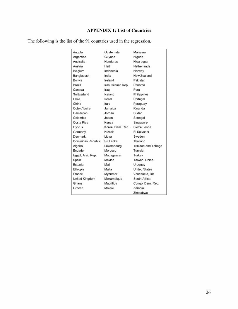
26

APPENDIX 1: List of Countries The following is the list of the 91 countries used in the regression.

Angola Guatemala Malaysia Argentina Guyana Nigeria Australia Honduras Nicaragua Austria Haiti Netherlands Belgium Indonesia Norway Bangladesh India New Zealand Bolivia Ireland Pakistan Brazil Iran, Islamic Rep. Panama Canada Iraq Peru Switzerland Iceland Philippines Chile Israel Portugal China Italy Paraguay Cote d'Ivoire Jamaica Rwanda Cameroon Jordan Sudan Colombia Japan Senegal Costa Rica Kenya Singapore Cyprus Korea, Dem. Rep. Sierra Leone Germany Kuwait El Salvador Denmark Libya Sweden Dominican Republic Sri Lanka Thailand Algeria Luxembourg Trinidad and Tobago Ecuador Morocco Tunisia Egypt, Arab Rep. Madagascar Turkey Spain Mexico Taiwan, China Estonia Mali Uruguay Ethiopia Malta United States France Myanmar Venezuela, RB United Kingdom Mozambique South Africa Ghana Mauritius Congo, Dem. Rep. Greece Malawi Zambia Zimbabwe