an intermodal transport network planning algorithm using dynamic programming—a case study:...

Appl Intell (2012) 36:529–541DOI 10.1007/s10489-010-0223-6

An intermodal transport network planning algorithmusing dynamic programming—A case study:from Busan to Rotterdam in intermodal freight routing

Jae Hyung Cho · Hyun Soo Kim · Hyung Rim Choi

Published online: 25 March 2010© Springer Science+Business Media, LLC 2010

Abstract This paper presents a dynamic programming al-gorithm to draw optimal intermodal freight routing with re-gard to international logistics of container cargo for exportand import. This study looks into the characteristics of inter-modal transport using multi-modes, and presents a WeightedConstrained Shortest Path Problem (WCSPP) model. Thisstudy draws Pareto optimal solutions that can simultane-ously meet two objective functions by applying the LabelSetting algorithm, a type of Dynamic Programming algo-rithms, after setting the feasible area. To improve the algo-rithm performance, pruning rules have also been presented.The algorithm is applied to real transport paths from Bu-san to Rotterdam, as well as to large-scale cases. This studyquantitatively measures the savings in both transport costand time by comparing single transport modes with inter-modal transport paths. Last, this study applies a mathemati-cal model and MADM model to the multiple Pareto optimalsolutions to estimate the solutions.

Keywords Intermodal freight routing problem · Dynamicprogramming · Weighted constrained shortest pathproblem · Label setting algorithm

J.H. ChoSchool of International Business and Area Studies,Pusan University of Foreign Studies, 55-1 Uam-dong, Nam-gu,Busan 608-738, South Koreae-mail: [email protected]

H.S. Kim (�) · H.R. ChoiDepartment of Management Information Systems,Dong-A University, 1, 2-ga, Bumin-dong, Seo-gu,Busan 602-760, South Koreae-mail: [email protected]

H.R. Choie-mail: [email protected]

1 Introduction

In general, ordinary transport means a single transport modeby carrier. However, intermodal freight transportation canbe defined as the movement of cargoes from origins to des-tinations using two or more transportation modes such asair, ocean, rail, and road [1, 2, 4, 5, 14–16, 18]. Third-party logistics companies play important roles in intermodaltransport [1–3], because international logistics costs may ac-count for 30–50% of a company’s total production cost [14].A third-party logistics company is required to be equippedwith NPS (Network Planning System), NOS (Network Op-timization System), and DSS (Decision Support System).However, most companies are unable to provide enough in-formation, because they lack such systems. That can causeincreasing cost to consignors [4, 5]. Transport network plan-ning by manual work is therefore likely to pose problemswhen cargo volume carried by intermodal transport is in-creasing. Therefore, intermodal transport solutions have tobe easy to implement, flexible, reliable, transparent, and ef-ficient [16].

To solve this problem, i.e. to support the common inter-ests of the consignors and the third-party logistics compa-nies, it is necessary to build systems that can integrate themodes of transport, routing, and scheduling for intermodaltransport planning. Therefore, developing an efficient algo-rithm for intermodal transport planning is very necessary forintermodal operators such as consignors, shippers, transportagents, etc. This study suggests such an algorithm using DP(Dynamic Programming), which is one of many approachessolving WCSPP (Weighted Constrained Shortest Path Prob-lem) efficiently [19, 20]. WCSPP requires considering boththe cost and the weight constraint, such as time. We sug-gest a Dynamic Programming algorithm, which utilizessubstructures of the original problem, for Pareto optimal

mailto:[email protected]



530 J.H. Cho et al.

transport paths among many routing paths so consignors canminimize transport cost and time simultaneously. As a Dy-namic Programming algorithm, this study has selected theLabel Setting Algorithm (LSA) for the constrained shortestpath problem, because this algorithm developed in [12] isregarded as the most effective Dynamic Programming ap-proach algorithm for the WCSPP.

In addition, to simplify the numerous routing paths, prun-ing rules have also been presented. To test their efficacy,we have applied them to the actual intermodal transportpath from Busan, a Korean port, to Rotterdam, a port inthe Netherlands, through both small- and large-scale exper-iments.

2 International intermodal freight routing problem

Macharis and Bontekoning [5] and Jang and Kim [6] pointedout that Intermodal Freight Routing Problem (IFRP) wasnot actively studied in the optimization research field. Evenworse, the studies dealing with International IntermodalFreight Routing Problem (IIFRP) were not numerous, be-cause one of the difficulties studies in IIFRP face is to obtaina wide and deep knowledge about transport services, routes,fares, etc. Another crucial point is that it is difficult to definean optimum respecting the numerous objectives [16]. There-fore, Macharis and Bontekoning [5] argued that intermodalfreight transport research is emerging as a new transporta-tion research application field. IIFRP is defined as shortestpath problems with time windows (SPPTW) [12], as vehi-cle routing problems with time windows (VPRTW) [16],and/or as multi-objective multimodal multi-commodity flowproblem (MMMFP) [14] in each research. However, interna-tional intermodal routing is complicated by three importantcharacteristics of the most significant problem as follows:

1. multiple objectives such as minimization of travel timeand of travel cost

2. two or more scheduled transportation modes (means)such as air, ocean, rail, and road

3. one or more constraints related to time, cost, capacity ofmode or node, etc.

We will cover all of these three characteristics. Therefore,the problem is formulated in this paper as a multi-objectiveintermodal (multimodal) routing problem with time win-dows.

In the Min’s study (a representative study dealing withIIFRP), a chance-constraint objective planning model waspresented to select the most effective transportation modein terms of service cost among trucks, airlines, and ships,but used virtual data [2]. Jang and Kim [6] studied IIFRPto achieve efficiency in transport cost and time using a ge-netic algorithm, but it was limited to domestic intermodal

freight routing problems limited to one region and consid-ering only trucks as the transportation mode, and ship as atransshipment mode. Boardman et al. [4] and Barnhart andDonald [1] consider only multiple objectives.

In international transportation, a single mode can be used.Ships will be used when cargo volumes are large, deliverydue date is not so tight, and low transportation costs areneeded. Airlines will be preferred in cases where cargo isexpensive, and a tight delivery schedule is required, thoughthe freight is quite high. Anyway, if intermodal transport ismore economical in terms of cost and time, the usage of thisalgorithm will be on the rise.

For the transportation modes studied previously, Min [2]considers trucks, airlines, and ships; Barnhart and Don-ald [1] take into account trucks and ships. Boardman etal. [4] deal with trucks, trains, and airlines. In the currentliterature, Caramia and Guerriero [16] consider only trucksand trains. Southworth and Peterson [17] take into accounttrucks, trains, and ships. Chang [14] covers trucks, airlines,ships, and trains. Chang’s work is the one most related to ourwork in terms of research target. All these focused on effi-cient connectivity of various inland (domestic) transporta-tion modes with the international ones.

In contrast, this study focuses on international intermodaltransportation modes first. This is because the schedules ofinland transportation modes are made by private contractsbetween consignors and transporters, while international in-termodal transportation modes are operated in compliancewith open schedules. Therefore, it is realistic for a con-signor to decide upon international intermodal transporta-tion modes first, and then inland transportation modes next,in order to move his/her cargo. This study considers the ship,the train, and the airline as international intermodal trans-portations, and has developed an optimal transport algorithmbased on real intermodal freight routing from Busan to Rot-terdam. It has evaluated intermodal transport paths consid-ering not only transportation cost, but also time, in drawingan optimal intermodal transport path.

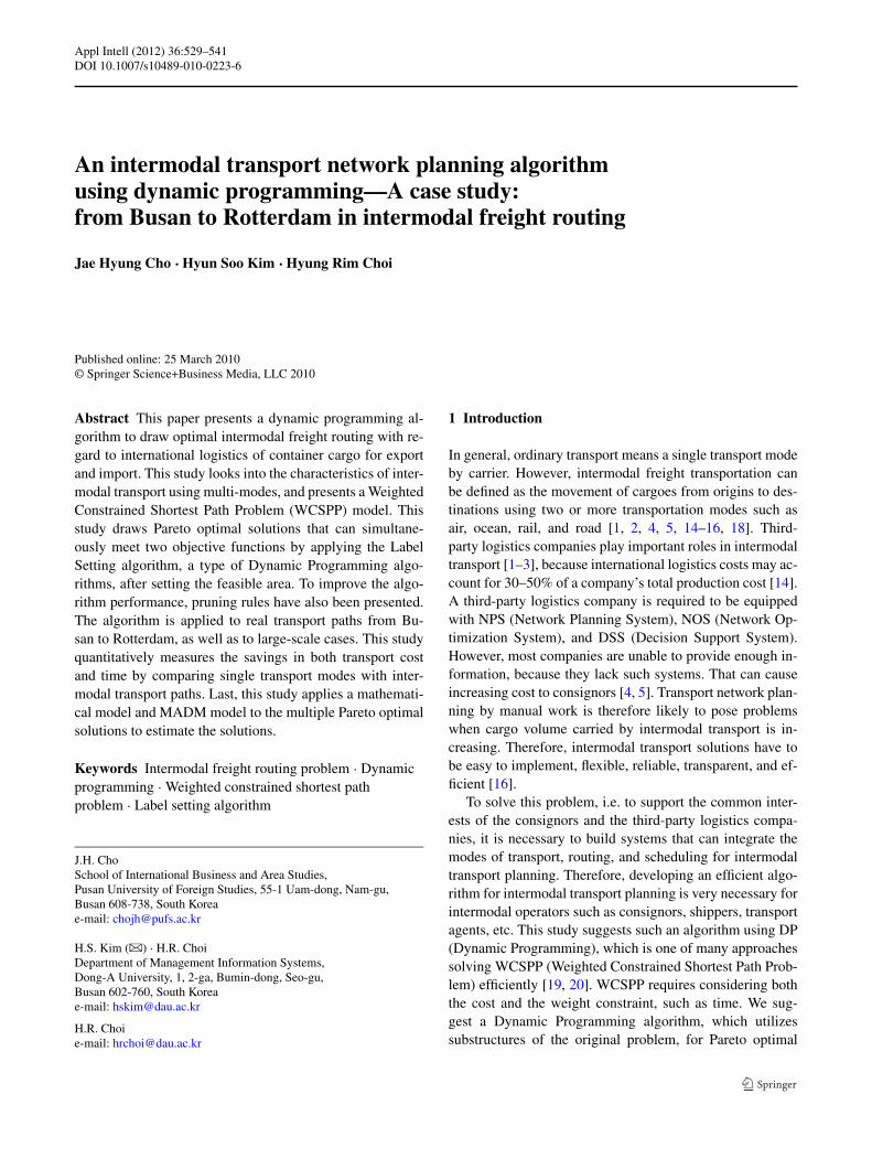
During cargo loading, all cargo needs to be loaded to-gether in the mode of transport. If there is a mode of trans-port that cannot be loaded by a unit of cargo, it will be pre-cluded in the route generation. In addition, the modes oftransport inclusive of the ship, the airplane, and the trainhave different destinations—harbor, airport, and station—which become the nodal points. Transshipment between dif-ferent transport modes can be made at the “location,” andwith multiple nodes in the one location, transshipment canbe made only once in the same location. Transshipment intothe other transport modes may be allowed only by land. Thetransportation cost and time by land are proportional to dis-tance. The definition of route components under the consid-eration of intermodal transport is shown in Fig. 1.

An intermodal transport network planning algorithm using dynamic programming—a case study 531

Fig. 1 Definition of routecomponents in intermodaltransport

3 Optimal intermodal transport network planningalgorithm

3.1 Pruning rules

This study has used a pruning algorithm which serves to im-prove performance and efficacy while seeking an optimalpath from among the numerous available paths for inter-modal transport to operate. This is because each arc can betraversed by different transportation modes or by a differ-ent scheduled mode in the same transportation mode, thusgenerating a multimodal multigraph.

If there are two arcs of “k” and “l” in one node (n), thetransport cost (C) and transport time (T ) comprise one pair:(Ck

n,T kn ) and (Cl

n, Tln). In addition, if one is in a dominant

position, the other arc will be eliminated by the pruningrules. The pruning rules are as follows.

Rule 1 The arc with a higher cost and time in one node willbe eliminated.

If Cln > Ck

n and T ln > T k

n , (Cln, T

ln) is eliminated

by (Ckn,T k

n )

Rule 2 If the cost of both arcs is the same in one node, butthe time is different, then the arc with the longer time iseliminated. In addition, if the time is the same, but their costis different, the higher-cost arc is to be eliminated.

If (Cln = Ck

n and T ln > T k

n ) or (T ln = T k

n andCl

n > Ckn), (Cl

n, Tln) is eliminated by (Ck

n,T kn )

Rule 3 If an arc in a node has an arrival date later than thelatest departure date, it is to be eliminated.

max(Sδ+n ) < (Aδ−

n )

If there is a departure arc (δ+) and arrival arc (δ−) in anode, and the departure time of the departure arc is repre-sented as Sδ+

n and the arrival time of the arrival arc is repre-sented as Aδ−

n , the arc Aδ−n is larger than the maximum value

of Sδ+n so it is to be eliminated.

3.2 Mathematical formulation of WCSPP

The constrained shortest path problem, which is an extendedshortest path problem, is generally known as the NP-hardproblem [14]. Taking account of the trade-off relationshipbetween time and cost, Martins discovered multiple Paretooptimal paths, solving the problem by way of combinationand optimization [7, 8, 16]. However, simultaneous consid-eration of two kinds of an objective function takes a longtime to calculate, but he also proved that it was impossi-ble to test all of Pareto’s optimal solutions. Due to this, letthere be only one objective function, and the other consider-ations be constraints. Based on this proposition, the shortestpath problem was actively being researched. These studiesare known as WCSPP (Weighted Constrained Shortest PathProblem) [9–11]. The objective function of WCSPP LinearProgram Formulation-based International Intermodal Trans-port, its constraints, and variables are defined as follows.

min∑

a∈A

(cma · qa · xm

a + qa · lcan + qa · uca

n

)

such that∑

a∈δ+(i)

xa −∑

a∈δ−(i)

xa

=⎧⎨

⎩

1, if i = s

−1, if i = t

0, if i ∈ V \{s, t}∀i ∈ V

∑

a∈A

waxa ≤ Wt xa ∈ {0,1} ∀a ∈ A

(1)

532 J.H. Cho et al.

min∑

a∈A

(tma · xm

a + ltan + utan)

such that∑

a∈δ+(i)

xa −∑

a∈δ−(i)

xa

=⎧⎨

⎩

1, if i = s

−1, if i = t

0, if i ∈ V \{s, t}∀i ∈ V

∑

a∈A

waxa ≤ Wc xa ∈ {0,1} ∀a ∈ A

(2)

cma : Transport cost of transport mode m at arc a

xma : When transported from arc a by transport mode m,

1 or 0qa : Quantity of cargo at arc a

lcan: Loading cost of arc a at node n

ucan: Unloading cost of arc a at node n

ltan: Loading time of arc a at node n

tma : Transport time of transport mode m at arc a

utan: Unloading time of arc a at node n

wa : Constraint at arc a

Wc: Cost constraintWt : Time constraint

The objective function of a WCSPP LP model, whichtook intermodal transport into account, can be defined asfollows:

The objective function which minimizes cost as in (1)considered transportation cost at the arc and loading/unload-ing cost at the node; quantity of freight was included, be-cause cost is in proportion with quantity of freight. Whenminimizing time as in the objective function in (2), not onlytransportation time from one node to another, but also load-ing time at a point of departure, unloading time at a point ofarrival, and transshipment time (loading/unloading) at tran-sits were considered.

The constraints of (1) and (2) are the same form, but theconstraint Wt in (1) is time, and the constraint Wc in (2) iscost.

There exist many different approaches for solving WC-SPP. They are label setting algorithm from dynamic pro-gramming approach, and methods based on Lagrangian Re-laxation (LR) of the weight constraint. LR-approach cangive us both lower bound and upper bound on the optimalsolution and it is a good candidate if our routing query onlywants an approximation on the cost from departure to desti-nation city given time constraint. However, it requires somepre-processing work on converting the graph into linear pro-gram formulation. Consequently, in terms of routing query,if the data is frequently updated, then, upon each updatetime, we need to re-generate the LP-form for the new graph,which is a costly operation. Therefore, we will adopt dy-namic programming approach (DP), because dynamic pro-gramming approach is easier to understand and implement.Also, it enjoys the best worst-case time complexity [6]. Theworst-case complexity of DP is O(|A|∗W), where |A| is thesize of the arc set and W is the weight limit of the WCSPP.

3.3 Dynamic programming for WCSPP

Equations (1) and (2) can bring the points Z2 and Z1 asshown in Fig. 2 respectively. Z3, at the intersection of thesetwo points, seems to be an ideal optimal solution for the twoobjective functions. But Z3 is an infeasible solution.

Accordingly, we have defined the area (shaded area) inthe three points as the effective area. So if the solution ofthe DP algorithm lies in the effective area, it will becomean effective solution. The feasible solutions are subset of theeffective solution set. The range between T1 and T2 in theeffective area is defined as an ‘effective time range,’ whichbecomes the time constraint range in the DP algorithm forminimizing cost.

Fig. 2 The feasible area ofWCSPP algorithm


Fig. 3 Major intermodal transport nodes between Busan and Rotterdam using ships

As a solution for the DP algorithm, this study has used theLabel Setting algorithm. The Label Setting algorithm wasdeveloped by Descrochers and Soumis [12]. This methodattaches labels to each node, and the labels are composedof a pair {weight, objective function}. In the Label Settingalgorithm, time was weighted as a constraint and cost wasexpressed as the objective function. Therefore, the effectivetime range obtained in the WCSPP LP model is imposed asthe weight of the Label Setting algorithm.

In the label {Wqi ,C

qi }, W

qi refers to the qth weight in

the node i, and Cqi refers to the qth cost in the node i. wij

and cij refer to the weight and cost from node i to node j ,respectively. The Label Setting algorithm is generally per-formed as follows.

Step 0: InitializationSet Labels = {(0,0)}, and set Labeli = � for all i ∈V \{s}.

Step 1: Selection of the label to be extendedIf all Labels have been marked, then TERMINATE;all efficient labels have been generated;Else choose i ∈ V such that there’s unmarked labelin Labeli and W

qi is minimal, where q is the path

that attains this weight valueStep 2: Extend label (Wq

i ,Cqi )

For all (i, j) ∈ δ+(i) with Wqi + wij ≤ W do

Table 1 Major intermodal transport paths between Busan and Rotter-dam

Transportation mode Intermodal Transport Paths

Ship + railwayor railway

– TSR (Trans Siberian Railway)

– TCR (Trans China Railway)

– TMR (Trans Manchuria Railway)

– TMGR (Trans Mongolia Railway)

– TKR (Trans Korea Railway)

Ship + aircarrier

– Busan port–(ship)–New York–(air)–

Rotterdam Airport

– Busan port–(ship)–LA–(air)–

Rotterdam Airport

If (Wqi +wij ,C

qi +cij ) is not dominated by (Wk

j ,Ckj )

for any existing label at node j

Then set Labelj = Labelj ∪{(Wqi +wij ,C

qi + cij )}

Mark label (Wqi ,C

qi )

Goto Step 1.

The Label Setting algorithm is easier to understand andimplement. In practice, in the case of a large network, largeproblem set, people usually use Label Setting algorithm,since it is easier to maintain the entire graph, and it is more

534 J.H. Cho et al.

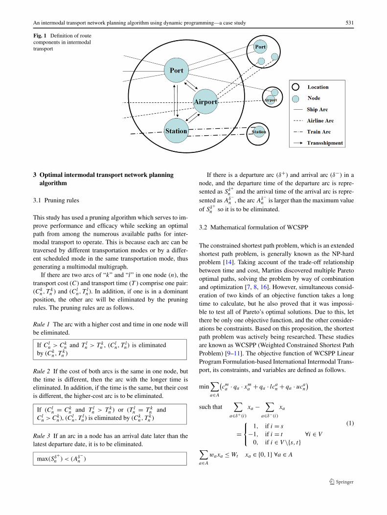
Fig. 4 Major intermodal transport nodes between Busan and Rotterdam using airlines and trains

Table 2 Transport time andcost of single transport modesbetween Busan and Rotterdam

Classification Transport mode Transport time Transport cost

Minimum cost Ship 600 hours $1600

Shortest time Truck–airplane 20 hours $35,800

efficient to update the data in a graph rather than convertinga graph into a linear program system.

4 Experiment

4.1 An illustrative experiment

Ships and Airlines are the single transportation modes fromBusan to Rotterdam. There were about 20 shipping sched-ules in the unit of a month (from Nov. 26, 2005 to Dec. 20,2005), while about 2–5 air flight schedule were provideddaily. This study has calculated transport costs based on thetwenty-foot equivalent unit (TEU, the unit of marine freightcontainer), and converted cubic meter (CBM, the unit of airfreight) from TEU.

The path to Rotterdam from Busan is a typical interna-tional trade channel between Asia and Europe. At present,

the major intermodal transport paths between these two ar-eas can be summarized as in Table 1. We assume the TKRis under operation through North Korea.

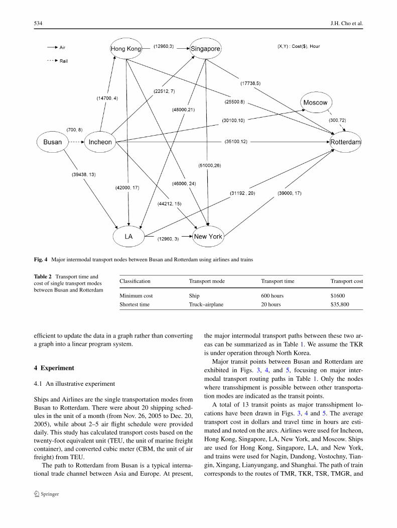
Major transit points between Busan and Rotterdam areexhibited in Figs. 3, 4, and 5, focusing on major inter-modal transport routing paths in Table 1. Only the nodeswhere transshipment is possible between other transporta-tion modes are indicated as the transit points.

A total of 13 transit points as major transshipment lo-cations have been drawn in Figs. 3, 4 and 5. The averagetransport cost in dollars and travel time in hours are esti-mated and noted on the arcs. Airlines were used for Incheon,Hong Kong, Singapore, LA, New York, and Moscow. Shipsare used for Hong Kong, Singapore, LA, and New York,and trains were used for Nagin, Dandong, Vostochny, Tian-gin, Xingang, Lianyungang, and Shanghai. The path of traincorresponds to the routes of TMR, TKR, TSR, TMGR, and


Fig. 5 Major intermodal transport nodes between Busan and Rotterdam using ships and trains

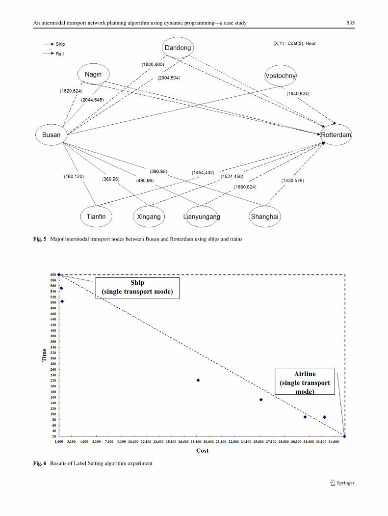
Fig. 6 Results of Label Setting algorithm experiment

536 J.H. Cho et al.

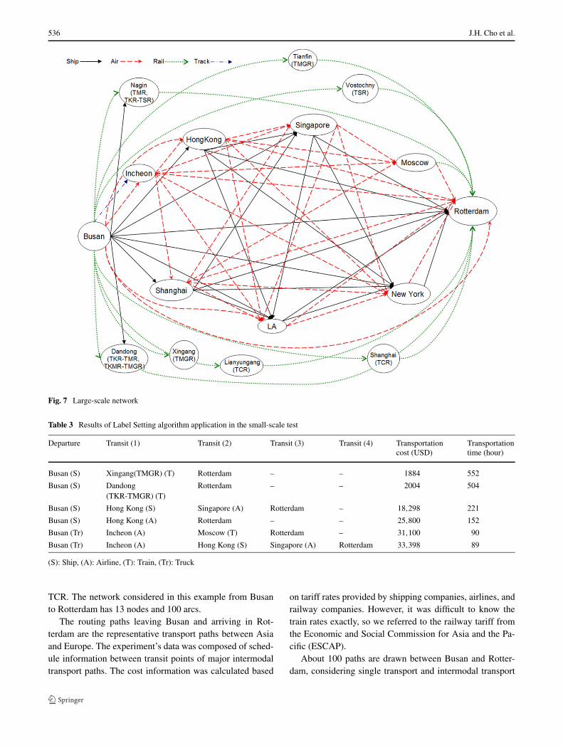
Fig. 7 Large-scale network

Table 3 Results of Label Setting algorithm application in the small-scale test

Departure Transit (1) Transit (2) Transit (3) Transit (4) Transportationcost (USD)

Transportationtime (hour)

Busan (S) Xingang(TMGR) (T) Rotterdam – – 1884 552

Busan (S) Dandong Rotterdam – – 2004 504(TKR-TMGR) (T)

Busan (S) Hong Kong (S) Singapore (A) Rotterdam – 18,298 221

Busan (S) Hong Kong (A) Rotterdam – – 25,800 152

Busan (Tr) Incheon (A) Moscow (T) Rotterdam – 31,100 90

Busan (Tr) Incheon (A) Hong Kong (S) Singapore (A) Rotterdam 33,398 89

(S): Ship, (A): Airline, (T): Train, (Tr): Truck

TCR. The network considered in this example from Busanto Rotterdam has 13 nodes and 100 arcs.

The routing paths leaving Busan and arriving in Rot-terdam are the representative transport paths between Asiaand Europe. The experiment’s data was composed of sched-ule information between transit points of major intermodaltransport paths. The cost information was calculated based

on tariff rates provided by shipping companies, airlines, andrailway companies. However, it was difficult to know thetrain rates exactly, so we referred to the railway tariff fromthe Economic and Social Commission for Asia and the Pa-cific (ESCAP).

About 100 paths are drawn between Busan and Rotter-dam, considering single transport and intermodal transport


Table 4 Results of Label Setting algorithm application in the large-scale test

Time constraint Departure Transit Transportationcost (USD)


More than1000 hours

O) Busan (S) Hong Kong 269 150

Hong Kong (S) Singapore 155 50

Singapore (S) D) Rotterdam 1000 460

Total 1424 660

Less than600 hours

O) Busan (S) D) Rotterdam 1600 600

Total 1600 600

Less than500 hours



Singapore (A) D) Rotterdam 14,000 8

Total 14,424 208

Less than200 hours

O) Busan (S) Shanghai 250 95

Shanghai (A) Moscow 16,000 5

Moscow (T) D) Rotterdam 300 3

Total 16,550 103

Less than100 hours

O) Busan (A) Hong Kong 13,800 5


Singapore (A) D) Rotterdam 14,000 8

Total 27,955 63

Less than50 hours

O) Busan (Tr) Incheon 700 8

Incheon (A) Shanghai 11,000 3

Shanghai (A) Moscow 16,000 5

Moscow (T) D) Rotterdam 300 3

Total 28,000 19

O): Origin, D): Destination, (S): Ship, (A): Airline, (T): Train, (Tr): Truck

modes simultaneously. We dealt with departure and arrivaltimes when applying the pruning rule. Due to the applicationof the pruning rules to the schedules, 11 paths were elimi-nated according to Pruning Rule 3.

Next, a WCSPP LP model was applied to the 89 paths.As a result, transport by ship incurred the minimum cost,while transport by airplane made the shortest time. Table 2exhibits the results.

The feasible area has been defined, based on the resultsdrawn in the WCSPP LP model. Last, the Label Setting al-gorithm, which is a DP algorithm, was carried out for 89paths. Due to the execution of the Label Setting algorithm,the paths deviating from the feasible areas have been re-moved again. The number of the paths that deviated was 81.Most of them executed four or more transshipments. Thosepaths transporting cargo by air more than once were alsoremoved. This is because loading and unloading costs andtime have relatively increased due to the frequent transship-ments. In planning an intermodal transport route with realdata, more than three transshipments rarely occurred.

Figure 6 indicates the solutions included in the effectivearea based on the time-cost coordinates by applying the La-

bel Setting algorithm, where the range of 20 to 600 hours arethe time constraints making sub-problems in the Label Set-ting algorithm. The solution paths exhibited in the coordi-nates are 8, and these are the values included in the effectivearea as in Fig. 2. These 8 solutions are the Pareto optimal.

As presented above, the minimum transportation costwas USD 1600, when freight was transported by the singleship transportation mode, and the transportation time took600 hours. In case of intermodal transport format the pathBusan–(ship)–Xingang–(train)–Rotterdam cost a minimumof USD 1884, and the transportation time took 552 hours.As a result of carrying out the Label Setting algorithm, inter-modal transport path did not draw a cheaper path comparedto single transportation by ship. However, when consider-ing the transportation cost along with transportation timetogether, the intermodal transport path had the competitiveedge. The Pareto paths are listed in Table 3.

4.2 A larger-scale experiment

In this larger-scale experiment, we added more nodes andarcs to the previous experiment to increase the size of the

538 J.H. Cho et al.

Table 5 Results of Label Setting algorithm application including mandatory node LA

Time constraint Departure Transit Transportationcost (USD)


More than1000 hours



Singapore (S) LA 1250 530

LA (S-1) D) Rotterdam 1600 360

Total 3274 1090


Total 3244 1095

Less than600 hours

O) Busan (S) New York 1000 295

New York (S) LA 1100 249


Total 3700 904


Total 3670 909

Less than500 hours

O) Busan (S) New York 1200 240

New York (S) LA 1100 249


Total 3900 849


Total 3870 854

LA (A) D) Rotterdam 31,192 20

Total 33,492 509

Less than400 hours

O) Busan (S) LA 2750 270


Total 4320 635


Total 4350 630

Less than300 hours

O) Busan (S) LA 2750 270


Total 33,942 290

Less than100 hours

O) Busan (A) LA 21,000 18


Total 52,192 38

O): Origin, D): Destination, (S-1): Ship 1, (S-2): Ship 2, (A): Airline

network. There are 14 transit nodes in the network afteradding Shanghai port, and we put 10 arcs for each adjacentnode. Figure 7 illustrates the network.

The setting of network showed a total number of arcs inthe experiment of 61,542,910. The cost and time of eacharc are randomly generated so that no arc can be dominatedby the pruning rules. Table 4 shows the result of the large-scale experiment by making the travel time as the dynamicconstraint of the Label Setting algorithm.

When time constraint is more than 1000 h, the pathBusan–(ship)–Hong Kong–(ship)–Singapore–(ship)–Rotter-dam is optimal, where the cost is USD 1424 and time is660 h. When the time constraint is between 900 and 700 h,the result is same with the case of 1000 h.

The algorithm of the study and experiments can be veryuseful to intermodal operators. Since the required cost andtime between source and destination nodes are easily ana-lyzed, intermodal operators can efficiently design the inter-


Table 6 Normalization of time and cost value for the evaluation ofPareto optimal solutions

Pareto optimal solutions Normalized value

(1600,600) (0.02418,0.59777)

(1884,552) (0.02848,0.55000)

(2004,504) (0.03029,0.50212)

(18298,221) (0.27656,0.22018)

(25800,152) (0.38995,0.15143)

(31100,90) (0.47006,0.08967)

(33398,89) (0.50479,0.08867)

(35800,20) (0.54110,0.19926)

Z3 (0.02418,0.01926)

Table 7 Evaluation result through the mathematical model

Pareto optimal solutions Distance from Z3

(1600,600) 0.50910

(1884,552) 0.46135

(2004,504) 0.41350

(18298,221) 0.28459

(25800,152) 0.37112

(31100,90) 0.44588

(33398,89) 0.48061

(35800,20) 0.52862

Z3 0.0

national intermodal routing. Second, the algorithm allowsadding a transit node that the intermodal operator wants toanalyze. That means if there is a node ‘A’ that should bepassed through in the path from the source node to destina-tion node, the algorithm can only consider paths that includethe ‘A.’ For example, the algorithm can generate optimalpaths from Busan to Rotterdam if we want to add LA anddecide the path should pass through LA. The experiment re-sult is shown in Table 5. These mandatory nodes becomeadditional constraints in generating a transport route.

4.3 Evaluation of Pareto optimal solutions

Effective intermodal solutions are required both to copewith the customers desiderata in terms of times, costs, re-liability and to take into account the consignors’ operationalneeds [15, 16]. Previous experiments show that the algo-rithm in this study can solve the multi-objective problem interms of time and cost. The next step is how we can evaluatethe multiple Pareto solutions if we should choose one amongthem, in other words, how a user (shipper or consignor) canselect one from among the 8 Pareto optimal solutions. So,the network operator should be capable of suggesting one

Table 8 Evaluation results of Pareto optimal solutions throughMADM

Pareto optimal solutions MADM evaluation results

(1600,600) 0.11123

(1884,552) 0.11708

(2004,504) 0.12347

(18298,221) 0.11040

(25800,152) 0.09574

(31100,90) 0.08725

(33398,89) 0.07991

(35800,20) 0.08184

Z3 0.19307

Table 9 Each attribute’s weight of MADM evaluation

Transportation cost Transportation time

0.55525 0.44476

Pareto solution that is closest to the ideal solution but infea-sible solution Z3 in Fig. 2.

If we can regard the generating phase of multiple Paretosolutions as a tactical phase, then selecting one solutionamong them is an operational phase. The operational phaseworks on the output of the tactical phase. However, the prob-lem is each user can have a different preference in terms oftime and cost. Therefore, in order to enable an effective se-lection, we can use two evaluation methods. To explain thetwo evaluation methods, let us use the 8 Pareto solutions inFig. 6.

The first is a mathematical model. Among the values ofthe straight lines connecting the Z3 point of an ideal optimalsolution and 8 Pareto optimal solutions, the shortest valuewill be evaluated as the optimal alternative. To that end, thevalue of time and cost has been normalized as in Table 6.

Table 6 shows the normalized values of the ideal optimalsolution Z3 and the 8 alternatives. As time and cost havea different size, their relative distribution is denoted as thevalues between 0 and 1. By using these normalized values,the user’s value for the 8 Pareto optimal solutions has beengenerated by using the distance from Z3, and the results areshown in Table 7.

By using the mathematical model, Table 7 shows that thehighly evaluated solution is (18298,221) because the dis-tance to Z3 is the shortest (minimum). That means the 4thsolution among the 8 Pareto optimal solutions is the best op-erable solution.

For the second evaluation method, we used MADM(Multi-Attribute Decision Making). By using MADM, manytrade-off attributes with different measuring criterion can benormalized in the single view of measure, so that each at-

540 J.H. Cho et al.

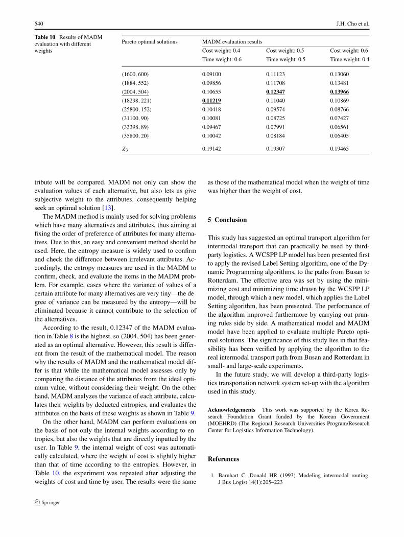
Table 10 Results of MADMevaluation with differentweights

Pareto optimal solutions MADM evaluation results

Cost weight: 0.4 Cost weight: 0.5 Cost weight: 0.6

Time weight: 0.6 Time weight: 0.5 Time weight: 0.4

(1600,600) 0.09100 0.11123 0.13060

(1884,552) 0.09856 0.11708 0.13481

(2004,504) 0.10655 0.12347 0.13966

(18298,221) 0.11219 0.11040 0.10869

(25800,152) 0.10418 0.09574 0.08766

(31100,90) 0.10081 0.08725 0.07427

(33398,89) 0.09467 0.07991 0.06561

(35800,20) 0.10042 0.08184 0.06405

Z3 0.19142 0.19307 0.19465

tribute will be compared. MADM not only can show theevaluation values of each alternative, but also lets us givesubjective weight to the attributes, consequently helpingseek an optimal solution [13].

The MADM method is mainly used for solving problemswhich have many alternatives and attributes, thus aiming atfixing the order of preference of attributes for many alterna-tives. Due to this, an easy and convenient method should beused. Here, the entropy measure is widely used to confirmand check the difference between irrelevant attributes. Ac-cordingly, the entropy measures are used in the MADM toconfirm, check, and evaluate the items in the MADM prob-lem. For example, cases where the variance of values of acertain attribute for many alternatives are very tiny—the de-gree of variance can be measured by the entropy—will beeliminated because it cannot contribute to the selection ofthe alternatives.

According to the result, 0.12347 of the MADM evalua-tion in Table 8 is the highest, so (2004,504) has been gener-ated as an optimal alternative. However, this result is differ-ent from the result of the mathematical model. The reasonwhy the results of MADM and the mathematical model dif-fer is that while the mathematical model assesses only bycomparing the distance of the attributes from the ideal opti-mum value, without considering their weight. On the otherhand, MADM analyzes the variance of each attribute, calcu-lates their weights by deducted entropies, and evaluates theattributes on the basis of these weights as shown in Table 9.

On the other hand, MADM can perform evaluations onthe basis of not only the internal weights according to en-tropies, but also the weights that are directly inputted by theuser. In Table 9, the internal weight of cost was automati-cally calculated, where the weight of cost is slightly higherthan that of time according to the entropies. However, inTable 10, the experiment was repeated after adjusting theweights of cost and time by user. The results were the same

as those of the mathematical model when the weight of timewas higher than the weight of cost.

5 Conclusion

This study has suggested an optimal transport algorithm forintermodal transport that can practically be used by third-party logistics. A WCSPP LP model has been presented firstto apply the revised Label Setting algorithm, one of the Dy-namic Programming algorithms, to the paths from Busan toRotterdam. The effective area was set by using the mini-mizing cost and minimizing time drawn by the WCSPP LPmodel, through which a new model, which applies the LabelSetting algorithm, has been presented. The performance ofthe algorithm improved furthermore by carrying out prun-ing rules side by side. A mathematical model and MADMmodel have been applied to evaluate multiple Pareto opti-mal solutions. The significance of this study lies in that fea-sibility has been verified by applying the algorithm to thereal intermodal transport path from Busan and Rotterdam insmall- and large-scale experiments.

In the future study, we will develop a third-party logis-tics transportation network system set-up with the algorithmused in this study.

Acknowledgements This work was supported by the Korea Re-search Foundation Grant funded by the Korean Government(MOEHRD) (The Regional Research Universities Program/ResearchCenter for Logistics Information Technology).

References

1. Barnhart C, Donald HR (1993) Modeling intermodal routing.J Bus Logist 14(1):205–223


2. Min H (1991) International intermodal choices via chance-constrained goal programming. Transp Res Part A: Gen25(6):351–362

3. Yu I, Kim J, Cho G, So S, Park Y (2004) Study on the evalua-tion standards to select third party logistics firms. J Korea InformStrategy Soc 8(1):579–584

4. Boardman BS, Malstrom EM, Butler DP, Cole MH (1997)Computer-assisted routing of intermodal shipments. Comput IndEng 33(1–2):311–314

5. Macharis C, Bontekoning YM (2004) Opportunities for OR inintermodal freight transport research: a review. Eur J Oper Res153:400–416

6. Jang Y, Kim E (2005) Study on the optimized model of intermodaltransport using genetic algorithm. Shipping Logist Res 45:75–98

7. Martins EQV (1984) On a multicriteria shortest path problem. EurJ Oper Res 1:236–245

8. Pasquale A, Maurizio B, Antonio S (2002) A penalty functionheuristic for the resource constrained shortest path problem. Eur JOper Res 142:221–230

9. Chen YL, Chin YH (1990) The quickest path problem. ComputOper Res 17(2):153–161

10. Moore MH (1976) On the fastest route for convey-type traffic inflowrate-contrained networks. Transp Sci 10:113–124

11. Rosen JB, Sun SZ, Xue GL (1991) Algorithm for the quickest pathproblem and the enumeration of quickest paths. Comput Oper Res18(6):579–584

12. Descrochers M, Soumis F (1988) A generalized permanent label-ing algorithm for the shortest path problem with time windows.INFOR 26:191–212

13. Hwang CL, Yoon KS (1981) Multiple attribute decision making:methods and applications. Lecture notes in economics and mathe-matical systems. Springer, Berlin

14. Chang TS (2008) Best routes selection in international intermodalnetworks. Comput Oper Res 35:2877–2891

15. Andersen J, Crainic TG, Christiansen M (2009) Service networkdesign with management and coordination of multiple fleets. EurJ Oper Res 193:377–389

16. Caramia M, Guerriero F (2009) A heuristic approach to long-haulfreight transportation with multiple objective functions. Omega37:600–614

17. Macharis C, Bontekoning YM (2004) Opportunities for OR in in-termodal freight transport research: a review. J Oper Res 153:400–416

18. Southworth F, Peterson BE (2000) Intermodal and internationalfreight network modeling. Transp Res Part C 8:147–166

19. Androutsopoulos KN, Zografos KG (2009) Solving the multi-criteria time-dependent routing and scheduling problem in a mul-timodal fixed scheduled network. J Oper Res 192:18–28

20. Dumitrescu I, Boland N (2001) Algorithms for the weight con-strained shortest path problem. Int Trans Oper Res 8(1):15–29

Jae Hyung Cho is an Instructorof SIBAS (School of InternationalBusiness and Area Studies) at Pu-san University of Foreign Stud-ies. He received his Ph.D. (2006)in Management Information Sys-tems from Dong-A University, Ko-rea. His current research interest in-cludes Agent systems and negotia-tion in the e-Business and Logistics.He won the Best Paper award at theInternational Society of Applied In-telligence (IAE/EIA-2007).

Hyun Soo Kim is a Professor ofDepartment of Management Infor-mation Systems at Dong-A Univer-sity. He received his Ph.D. fromKorea Advanced Institute of Sci-ence and Technology (KAIST) in1992. He has been a visiting scholarin the MSIS Department at Uni-versity of Texas at Austin (1997)and in the School of Computer Sci-ence at Carnegie Mellon University(2003). His primary research inter-ests are agent systems, logistics in-formation, and supply chain opti-mization. He has published papers

in Decision Support Systems, Computers & Industrial Engineering,Journal of Organizational Computing and Electronic Commerce, andFuzzy Sets and Systems. He has been listed in Marquis Who’s Who inthe world in the 2010 edition.

Hyung Rim Choi is a Professorof Department of Management In-formation Systems at Dong-A Uni-versity. He received his Ph.D. fromKorea Advanced Institute of Sci-ence and Technology (KAIST) in1993. His primary research inter-ests are port logistics informationsystems and operation algorithm.He has published papers in Artifi-cial Intelligence, Journal of Organi-zational Computing and ElectronicCommerce, and Computer & In-dustrial Engineering. He has beenlisted in Marquis Who’s Who in the

world, in Science and Engineering, in Asia as well as in IBC for out-standing scientists of the 21st century.

an intermodal transport network planning algorithm using dynamic programming—a case study:...

Documents