University of Pennsylvania University of Pennsylvania

ScholarlyCommons ScholarlyCommons

Summer Program for Undergraduate Research (SPUR) Wharton Undergraduate Research

2017

An Econometric Analysis in Retail Supply Chain Management: An Econometric Analysis in Retail Supply Chain Management:

Sales Forecasting, Inventory Benchmarking and Supply Chain Sales Forecasting, Inventory Benchmarking and Supply Chain

Optimization Optimization

Tolulope Adebayo University of Pennsylvania

Follow this and additional works at: https://repository.upenn.edu/spur

Part of the Operations and Supply Chain Management Commons

Recommended Citation Recommended Citation Adebayo, T. (2017). "An Econometric Analysis in Retail Supply Chain Management: Sales Forecasting, Inventory Benchmarking and Supply Chain Optimization," Summer Program for Undergraduate Research (SPUR). Available at https://repository.upenn.edu/spur/19

This paper is posted at ScholarlyCommons. https://repository.upenn.edu/spur/19 For more information, please contact repository@pobox.upenn.edu.

An Econometric Analysis in Retail Supply Chain Management: Sales Forecasting, An Econometric Analysis in Retail Supply Chain Management: Sales Forecasting, Inventory Benchmarking and Supply Chain Optimization Inventory Benchmarking and Supply Chain Optimization

Abstract Abstract The operational efficiency of a retailer is defined by its supply-chain management (SCM) mechanisms. When determining the efficiency of a retailer’s supply-chain management, the most commonly utilized metric is inventory turnover (IT). This econometric study systematically examines the relationship between SCM efficiency and IT rates by extracting inventory-based data for four global apparel retailers- Zara, Uniqlo, H&M, and Gap. The theoretical purpose of this study is to link quantitative analytics of top-grossing apparel retailers to operational conclusions.

Keywords Keywords supply-chain management (SCM), efficiency, inventory turnovers (IT), econometrics, global apparel retailers

Disciplines Disciplines Operations and Supply Chain Management

This working paper is available at ScholarlyCommons: https://repository.upenn.edu/spur/19

1

An Econometric Analysis in Retail Supply Chain

Management: Sales Forecasting, Inventory

Benchmarking and Supply Chain Optimization

Tolulope Adebayo

Candidate for Bachelor of Science in Economics | Class of 2020

The Wharton School, University of Pennsylvania

E-mail: tadebayo@wharton.upenn.edu

Faculty Advisor: Marshall Fisher

Professor of Operations, Information and Decisions

The Wharton School, University of Pennsylvania E-mail:

fisher@wharton.upenn.edu

Research discipline: Econometrics – Supply Chain Management

Acknowledgements: The author would like to acknowledge additional

help and suggestions from Prof. Abba Kreiger, Kory Kantenga, and Dr.

Utsav Schurmans.

2

ABSTRACT

The operational efficiency of a retailer is defined by its supply-chain management (SCM)

mechanisms. When determining the efficiency of a retailer’s supply-chain management, the most

commonly utilized metric is inventory turnover (IT). This econometric study systematically

examines the relationship between SCM efficiency and IT rates by extracting inventory-based

data for four global apparel retailers- Zara, Uniqlo, H&M, and Gap. The theoretical purpose of

this study is to link quantitative analytics of top-grossing apparel retailers to operational

conclusions.

Keywords: supply-chain management (SCM), efficiency, inventory turnovers (IT),

econometrics, global apparel retailers

3

INTRODUCTION

Inventory turns, the ratio of a firm’s cost of goods sold to its average inventory level, is

commonly used to measure performance of inventory managers, compare inventory productivity

across retailers, and assess performance improvements over time (Gaur, Fisher, & Raman, 2005).

Inventory turns are used as a benchmarking technique which optimally evaluates the inventory

turnovers of a retailer, but the annual inventory turns of U.S. retailers varies widely across firms

and also within firms from one year to another. Note that inventory turns and inventory

turnovers are the same thing but for the sake of this paper, IT will be used to refer to both. In

order to evaluate the supply-chain of any top-grossing global apparel retailer, the financial and

operational data must be properly analyzed. In the field of econometrics with respect to SCM,

mathematical methods are utilized in describing the operational trends of retailers.

Zara vs. H&M vs. Uniqlo vs. Gap

The top grossing subsidiary of the Inditex group is Zara, while H&M is the top grossing

retail chain for Hennes & Mauritz, and Uniqlo is to Fast Retailing, and Gap is to Gap Inc. Zara's

strategy is to offer a higher number of available products than its competitors, allowing the

company to appeal to a broader number of customers with unique tastes. Part of H&M's strategy

has been to offer customers featured products that have been marketed as designer collaborations

with well-known names such as Versace and Alexander Wang, which offers customers

additional lines for purchase that are different from most designs of the company.

Uniqlo's distribution channels are heavily concentrated in its country of origin, Japan, and

possess a distribution strategy that has centered on the timing of its products' introductions into

stores, with new products created as a function not of quantity, but of demand. Gap Inc.’s

strategizes with a three-pronged approach. It aims the Old Navy brand at cost-conscious

4

consumers, the Gap line at trendy buyers, and the Banana Republic collection at consumers who

want clothing of higher quality (Fisher et al.2011). The latter portion of this paper will evaluate

which retailer among the “winners” is “winning” in terms of SCM.

LITERATURE REVIEW

Admittedly, there exists extensive literature on the relationship between SCM and IT.

Perhaps the longevity and popularity of the IT metric is due to the ease of calculations and public

financial data. Since inventory is now woven into the performance metric at every level of an

organization, it is imperative that this metric truly is indicative of an effective supply chain.

One metric that scholars have had experience using is adjusted inventory turns, AIT.

Gaur et al. (1999) relate inventory turnover performance with stock returns of US retailers and

prove the significantly positive correlation between average stock returns and average annual IT.

Similarly, Gaur et al. (2005) use financial data for retail firms to investigate the correlation of IT

with gross margin (GM), capital intensity (CI) and sales surprise (SS) in a longitudinal study.

They state that changes in inventory turnover cannot be directly interpreted as performance

improvement or deterioration because they may be caused by firm-specific and environmental

characteristics. Therefore, they propose a benchmarking methodology that combines IT, GM, CI

and SS to provide a metric of inventory productivity, which they term as adjusted inventory

turnover (AIT). Note that the method for adjusting inventory in this paper is similar to the

method used to adjust GDP for inflation and the method in finance to adjust financial returns for

risk premium.

This paper contributes to this research stream by extending Gaur et al. (2005) and Raman

and Fisher (2010). The latter portion of the paper implements statistical methods in real time in

order to translate quantifiable data into non-quantified conclusions. The results of this paper are

5

useful to retailers to assess their performance changes over time. The over-arching goal of this

paper is to notify retailers that if demand is forecasted accurately, far enough in advance, it can

enable mass production under push control and lead to well managed inventories, lower

markdowns, higher profitability (gross margins), and value creation for shareholders in the short

and long term.

DATA

The purpose of this econometric study is to use quantitative methods on inventory-based

data to create qualitative conclusions about SCM. The most accepted measurement of SCM

worldwide is IT, so the idea is to have a measurement of IT as the dependent variable. Since all

of the retailers in the study come from different countries with different sizes of economy,

measuring IT USD will produce the most controlled results. The dependent variable for this

study is IT since the test is to see which retailer has the most effective SCM. The independent

variables for this study are gross margin/ markup (GM/MU), capital intensity (CI), and sales

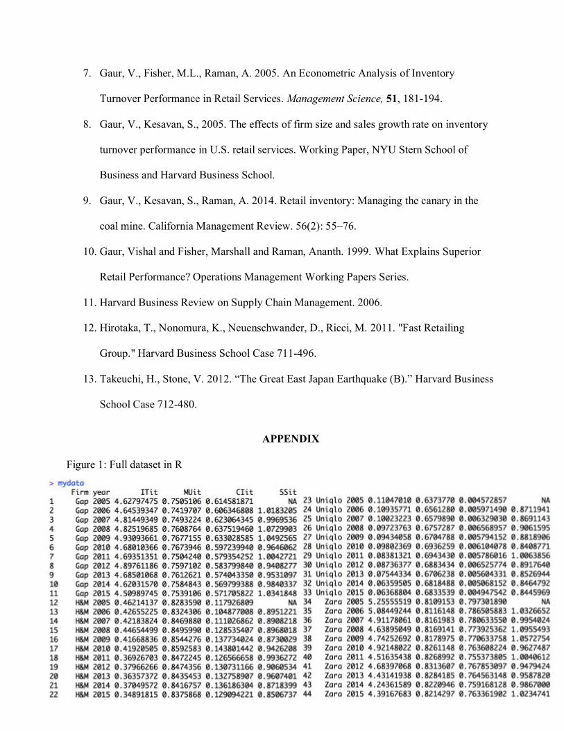
surprise (SS). Each variable is for firm i in year t. Gap serves as i=1, H&M is i=2, Uniqlo is i=3,

and Zara is i=4. The year of data decided upon for each variable ranged from 2005 to 2015, with

t=0 being 2005 and t=10 being 2015. The unit of measure that was taken as a standard for these

purposes is millions of USD and a range of data from 2005 to 2015 was used. This paper uses the

following currency conversions for all calculations: 1 SEK = 0.11 USD, 1 JPY= 0.009 USD and

1 EUR= 1.12 USD.

All of the collected data sets were acquired from Compustat - Capital IQ from Standard

& Poor's, both North America and Global (See Figure 1 for full dataset). This database pulls

index data from all publicly traded retailers, encompassing the full spectrum of inventory-based

data that could evaluate a supply chain.

6

“Phase A”

For this econometric study, there were two phases of data analysis entitled “Phase A” and

“Phase B”. For Phase A, the econometric was modeled after Gaur, Fisher and Raman (2005).

In the study, financial data for all publicly listed U.S. retailers for the 16-year period 1985–2000,

obtained from Standard & Poor’s Compustat database using the Wharton Research Data Services

(WRDS). The study identifies three variables that should be correlated with IT and can be

measured from public financial data: GM, CI (the ratio of average fixed assets to average total

assets), and SS (the ratio of actual sales to expected sales for the year). Their study uses results

from existing literature in order to formulate the following hypotheses to relate these variables to

IT.

Hypothesis 1: Inventory turnover is negatively correlated with gross margin.

Hypothesis 2. Higher capital intensity increases inventory turnover.

Hypothesis 3. Inventory turnover is positively correlated with sales surprise.

The results of their study gave a tradeoff curve that computes the expected IT of a firm for given

values of SS, GM, and CI. The term they used to define the distance of the firm from its tradeoff

curve was Adjusted Inventory Turnover, denoted AIT. They found that the value of AIT for firm

i in segment s in year t is comprised as:

AITsit = (ITsit) (GMsit)-b1 (CIsit)-b2 (SSsit)-b3

The following logarithm is used in “Phase A” of this study:

log(AITit)= log{(ITit) (GMit) (CIit) (SSit)}

The only difference between the former logarithm and the latter is that the former had segment-

specific coefficient estimates (b1, b2, b3). The latter logarithm disregards segment-specific

7

coefficient estimates because heterogeneity across retailing segments has already been

established.

By establishing the relationship between IT and GM, CI, and SS, the paper shows how IT

are an efficient measure of supply chain management. From their data, this paper computes the

following performance variables for “Phase A”:

Inventory turnover, ITit = CGSit

1

4 ΣInvit

Gross margin, GMit = Sit - CGSit

Sit

Capital intensity, CIit = ΣGFAit1

4 ΣInvit

Sales surprise, SSit = CGSit

1

4 ΣInvit

According to their study, CGSit denotes the cost of goods sold of firm i in year t;

Invit denotes the inventory valued at cost of firm i in year t; Sit is the sales, net of markdowns of

firm i in year t; GFAit is the gross fixed assets, comprised of land, property, and equipment of

firm i in year t. For SSit, refer to Holt’s Linear Smoothing Method. For more reference on

methodology for this study, refer to (Gaur, Fisher, & Raman, 2005). Once all the variables have

been analyzed, they are averaged together to produce a singular quantitative metric.

“Phase B”

“Phase B” was modeled after the following pooled model in (Fisher and Raman 2010).

The pooled model ignores the differences among various retailing segments.

8

The pooled model that was used for “Phase B” is almost identical to the equation above. The

only difference is the coefficient on the dependent variables. Some of the variables in the model

above are identical to the “Phase A” variables. The only new variables are:

Fi = Fixed effect for firm i

ct = Fixed effect for year t

eit = residual in the equation for firm i in year t

In words, the logarithm of inventory turns for a firm is a function of the markup (MU), capital

intensity (CI), and sales surprise (SS) for a particular firm in a particular year.

In panel data, individuals (persons, firms, cities, ...) are observed at several points in time

(days, years, before and after treatment, ...). Panel data is most useful when it is suspected that

the outcome variable depends on explanatory variables which are not observable but correlated

with the observed explanatory variables. In the random effects model, the individual-specific

effect is a random variable that is uncorrelated with the explanatory variables. In the fixed effects

model, the individual-specific effect is a random variable that is allowed to be correlated with the

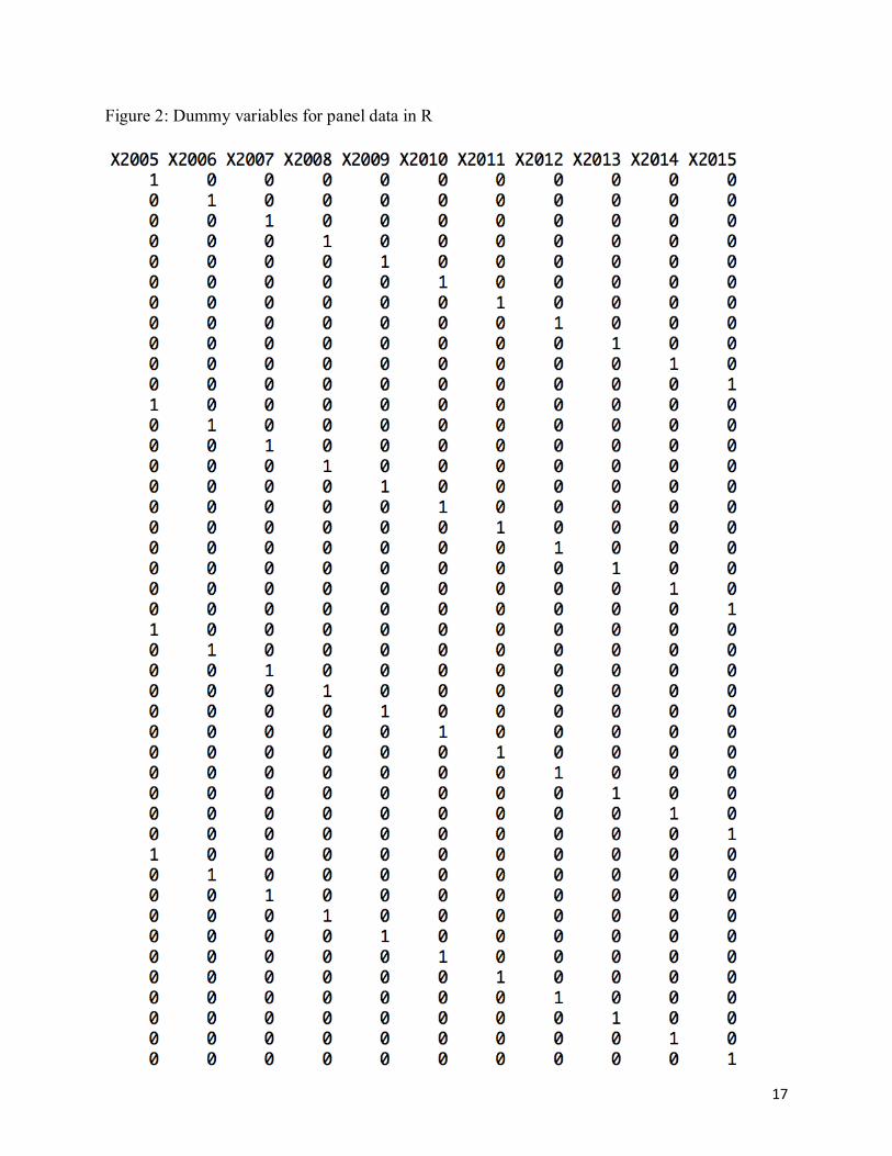
explanatory variables (Schmidheiny 2016). Therefore, a oneway fixed effects regression was run

with dummy variables for the year using the plm package (See Figure 2). The plm package is a

slightly modified version of Croissant and Millo (2008), published in the Journal of Statistical

Software. Plm is a package for R which intends to make the estimation of linear panel models

straightforward. Plm provides functions to estimate a wide variety of models and to make (robust)

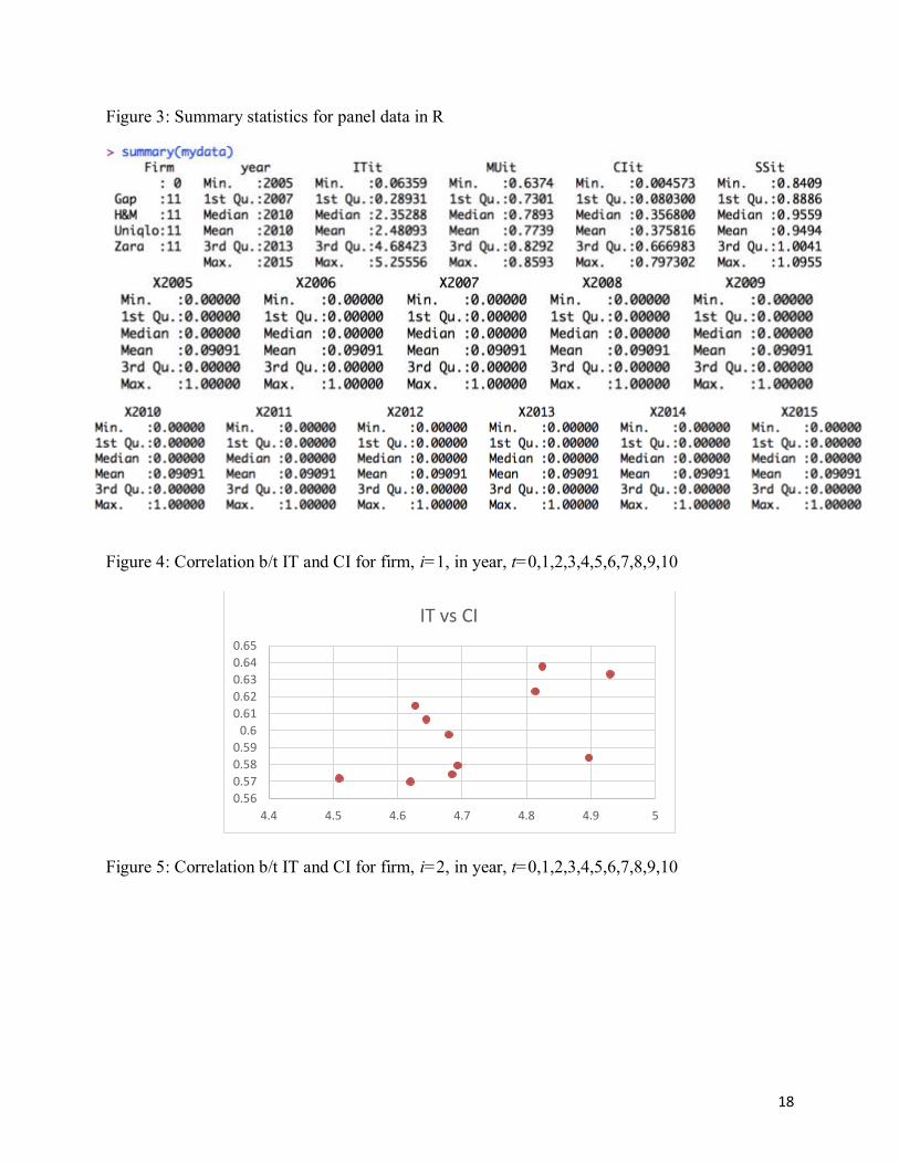
inference. See Figure 3 for the summary statistics for the entire dataset.

Independent vs. Dependent variables

Below are some graphs of the scatterplots between our dependent variable (IT) and the

independent variables (GM/MU, CI, and SS). Note that both “Phase A” and “Phase B” have

9

identical independent and dependent variables. Note that each blue dot represents a company-

year.

i=1, t=0,1,2,3,4,5,6,7,8,9,10

i=2, t=0,1,2,3,4,5,6,7,8,9,10

0.74

0.745

0.75

0.755

0.76

0.765

0.77

4.4 4.5 4.6 4.7 4.8 4.9 5

IT vs GM/MU

0.825

0.83

0.835

0.84

0.845

0.85

0.855

0.86

0.865

0 0.1 0.2 0.3 0.4 0.5

IT vs GM/MU

0.63

0.64

0.65

0.66

0.67

0.68

0.69

0.7

0 0.02 0.04 0.06 0.08 0.1 0.12

IT vs GM/MU

10

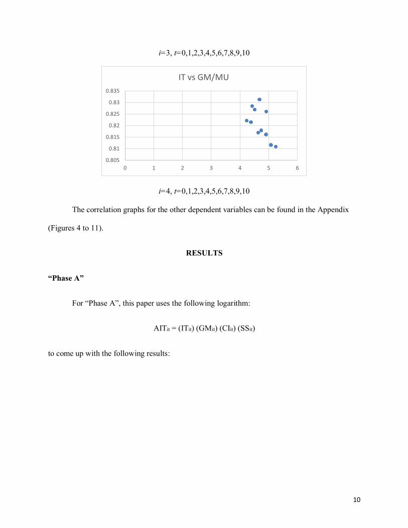
i=3, t=0,1,2,3,4,5,6,7,8,9,10

i=4, t=0,1,2,3,4,5,6,7,8,9,10

The correlation graphs for the other dependent variables can be found in the Appendix

(Figures 4 to 11).

RESULTS

“Phase A”

For “Phase A”, this paper uses the following logarithm:

AITit = (ITit) (GMit) (CIit) (SSit)

to come up with the following results:

0.805

0.81

0.815

0.82

0.825

0.83

0.835

0 1 2 3 4 5 6

IT vs GM/MU

11

12

“Phase B”

Below are the results to the oneway fixed effects regression from the following pooled

model.

logITit = Fi + ct +0.260225logMUit + 3.207849logCIit - 0.408557logSSit + eit

13

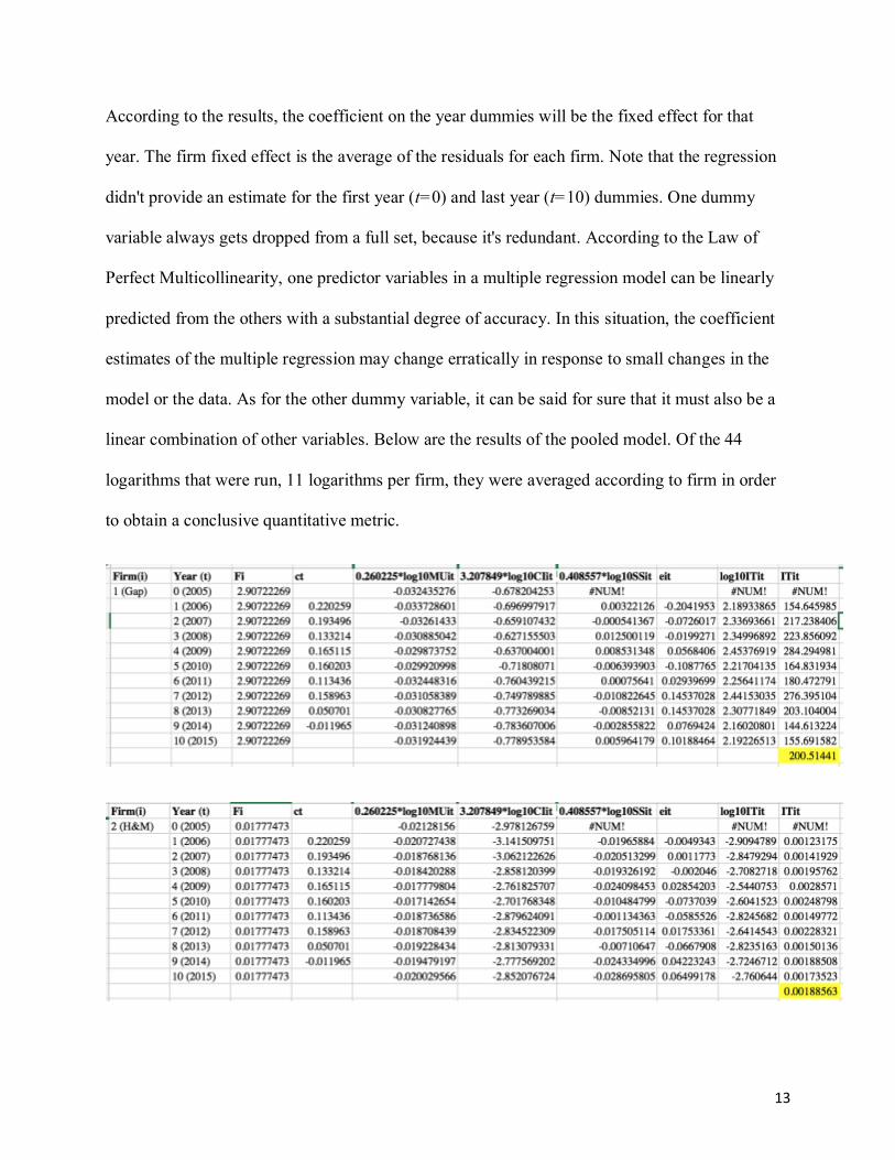
According to the results, the coefficient on the year dummies will be the fixed effect for that

year. The firm fixed effect is the average of the residuals for each firm. Note that the regression

didn't provide an estimate for the first year (t=0) and last year (t=10) dummies. One dummy

variable always gets dropped from a full set, because it's redundant. According to the Law of

Perfect Multicollinearity, one predictor variables in a multiple regression model can be linearly

predicted from the others with a substantial degree of accuracy. In this situation, the coefficient

estimates of the multiple regression may change erratically in response to small changes in the

model or the data. As for the other dummy variable, it can be said for sure that it must also be a

linear combination of other variables. Below are the results of the pooled model. Of the 44

logarithms that were run, 11 logarithms per firm, they were averaged according to firm in order

to obtain a conclusive quantitative metric.

14

CONCLUSIONS

By simultaneously analyzing other retailers and their respective inventory-based metrics,

it is evident that Zara has the highest average of AIT in “Phase A.” The results for “Phase B”

were the product of an oneway fixed effects regression from a pooled model, in which Gap had

the highest value of IT.

Moving forward several changes would be made. The first, and most important, change

would be to add more North American firms to the study. By doing so, the pool of public

financial data will be more immense and much more varied. By conducting a study with only

one North American firm, the current amount of public financial data was useful, but limited to

the public financial data of the global firms. By adding more North American retailers, there will

be more variations of logarithms and statistical methods. In addition to this, statistical

15

significance will be more evident once the sample size of the study increases by approximately

tenfold.

Due to the results of the quantitative analysis, another change should be implemented.

This change has to do with the concept of multicollinearity. When the oneway fixed effects

regression was run, an estimate for the first year (t=0) and last year (t=10) dummies was not

provided. According to this statistical concept, one dummy variable should always get dropped,

but in this case two dummy variables were dropped. By way of the concept, there are several

reasons as to why this phenomenon is caused. In the case of inaccurate use of dummy variables,

then a reconciliation of this would be recommended.

REFERENCES

1. Alan, Y., Gao, G., Gaur, V. 2014. Does Inventory Productivity Predict Future Stock

Returns? A Retailing Industry Perspective. Management Science 60(10):2416-2434.

2. Caro, F. 2012. Zara: Staying fast and fresh. The European Case Clearing House, ECCH

Case 612-006-1, Anderson School of Management, University of California, Los

Angeles, Los Angeles

3. Cox, E. 2011. Retail Analytics: The Secret Weapon, John Wiley & Sons, Incorporated,

4. Fisher, M.L., Hammond, J.H., Obermeyer, W.R., Raman, A. 1994. Making supply meet

demand in an uncertain world. Harvard Business Review. 72(3):83–93.

5. Fisher, M.L., Raman, A. 2010. The New Science of Retailing: How Analytics Are

Transforming the Supply Chain and Improving Performance. Harvard Business Press.

6. Gaur, V., Fisher, M.L., Raman, A., Stern, L. 2003. Retail Inventory Productivity:

Analysis and Benchmarking.

16

7. Gaur, V., Fisher, M.L., Raman, A. 2005. An Econometric Analysis of Inventory

Turnover Performance in Retail Services. Management Science, 51, 181-194.

8. Gaur, V., Kesavan, S., 2005. The effects of firm size and sales growth rate on inventory

turnover performance in U.S. retail services. Working Paper, NYU Stern School of

Business and Harvard Business School.

9. Gaur, V., Kesavan, S., Raman, A. 2014. Retail inventory: Managing the canary in the

coal mine. California Management Review. 56(2): 55–76.

10. Gaur, Vishal and Fisher, Marshall and Raman, Ananth. 1999. What Explains Superior

Retail Performance? Operations Management Working Papers Series.

11. Harvard Business Review on Supply Chain Management. 2006.

12. Hirotaka, T., Nonomura, K., Neuenschwander, D., Ricci, M. 2011. "Fast Retailing

Group." Harvard Business School Case 711-496.

13. Takeuchi, H., Stone, V. 2012. “The Great East Japan Earthquake (B).” Harvard Business

School Case 712-480.

APPENDIX

Figure 1: Full dataset in R

17

Figure 2: Dummy variables for panel data in R

18

Figure 3: Summary statistics for panel data in R

Figure 4: Correlation b/t IT and CI for firm, i=1, in year, t=0,1,2,3,4,5,6,7,8,9,10

Figure 5: Correlation b/t IT and CI for firm, i=2, in year, t=0,1,2,3,4,5,6,7,8,9,10

0.56

0.57

0.58

0.59

0.6

0.61

0.62

0.63

0.64

0.65

4.4 4.5 4.6 4.7 4.8 4.9 5

IT vs CI

19

Figure 6: Correlation b/t IT and CI for firm, i=3, in year, t=0,1,2,3,4,5,6,7,8,9,10

Figure 7: Correlation b/t IT and CI for firm, i=4, in year, t=0,1,2,3,4,5,6,7,8,9,10

Figure 8: Correlation b/t IT and SS for firm, i=1, in year, t=0,1,2,3,4,5,6,7,8,9,10

0

0.02

0.04

0.06

0.08

0.1

0.12

0.14

0.16

0 0.1 0.2 0.3 0.4 0.5

IT vs CI

0

0.001

0.002

0.003

0.004

0.005

0.006

0.007

0 0.02 0.04 0.06 0.08 0.1 0.12

IT vs CI

0.75

0.76

0.77

0.78

0.79

0.8

0 1 2 3 4 5 6

IT vs CI

20

Figure 9: Correlation b/t IT and SS for firm, i=2, in year, t=0,1,2,3,4,5,6,7,8,9,10

Figure 10: Correlation b/t IT and SS for firm, i=3, in year, t=0,1,2,3,4,5,6,7,8,9,10

Figure 11: Correlation b/t IT and SS for firm, i=4, in year, t=0,1,2,3,4,5,6,7,8,9,10

0.92

0.94

0.96

0.98

1

1.02

1.04

1.06

1.08

4.4 4.5 4.6 4.7 4.8 4.9 5

IT vs SS

0.84

0.86

0.88

0.9

0.92

0.94

0.96

0.98

1

1.02

0 0.1 0.2 0.3 0.4 0.5

IT vs SS

0.8

0.85

0.9

0.95

1

1.05

0 0.02 0.04 0.06 0.08 0.1 0.12

IT vs SS

21

0.9

0.95

1

1.05

1.1

1.15

0 1 2 3 4 5 6

IT vs SS