An brief introduction to Finsler geometry

Matias Dahl

July 12, 2006

Abstract

This work contains a short introduction to Finsler geometry. Special em-phasis is put on the Legendre transformation that connects Finsler geometrywith symplectic geometry.

Contents

1 Finsler geometry 31.1 Minkowski norms . . . . . . . . . . . . . . . . . . . . . . . 41.2 Legendre transformation . . . . . . . . . . . . . . . . . . . 6

2 Finsler geometry 92.1 The global Legendre transforms . . . . . . . . . . . . . . . 9

3 Geodesics 15

4 Horizontal and vertical decompositions 194.1 Applications . . . . . . . . . . . . . . . . . . . . . . . . . . 22

5 Finsler connections 255.1 Finsler connections . . . . . . . . . . . . . . . . . . . . . . 255.2 Covariant derivative . . . . . . . . . . . . . . . . . . . . . . 265.3 Some properties of basic Finsler quantities . . . . . . . . . . 27

6 Curvature 29

7 Symplectic geometry 317.1 Symplectic structure on T ∗M \ 0 . . . . . . . . . . . . . 337.2 Symplectic structure on TM \ 0 . . . . . . . . . . . . . . 34

1

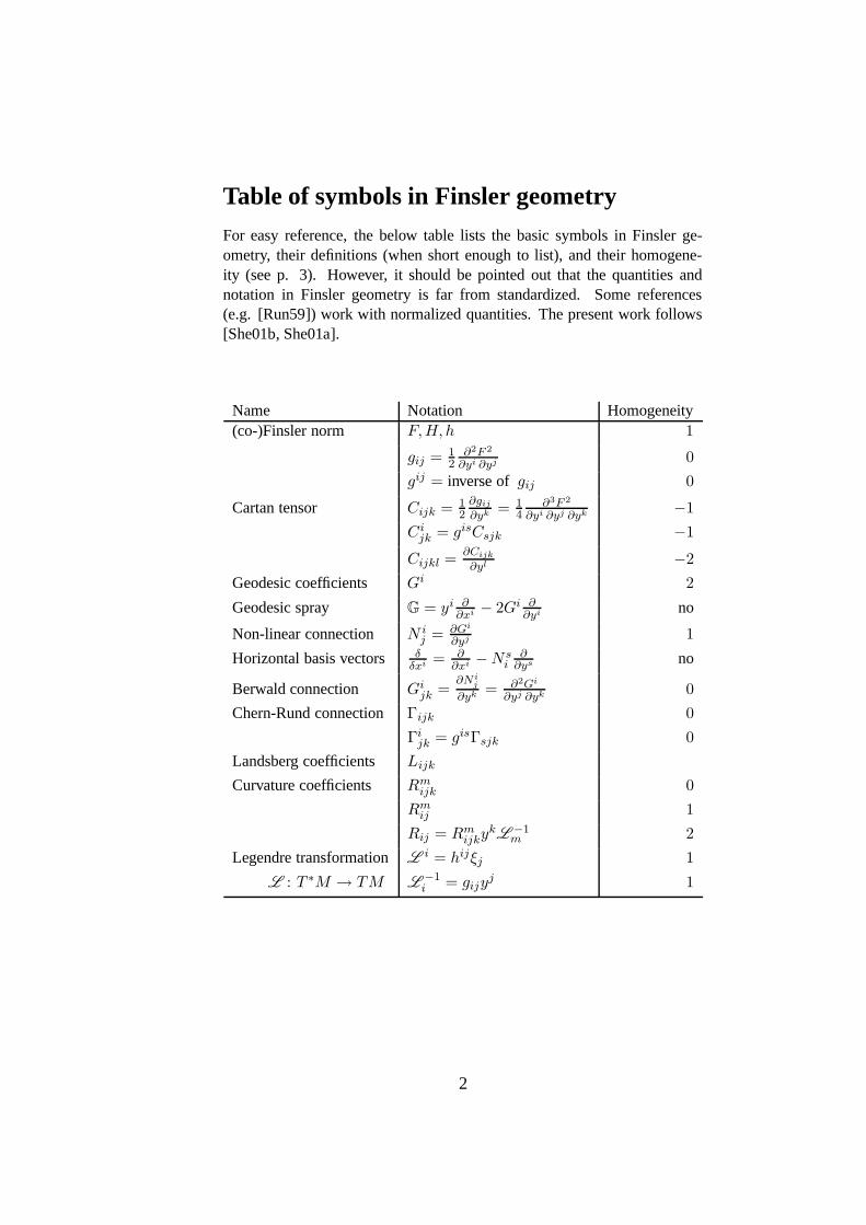
Table of symbols in Finsler geometry

For easy reference, the below table lists the basic symbols in Finsler ge-ometry, their definitions (when short enough to list), and their homogene-ity (see p. 3). However, it should be pointed out that the quantities andnotation in Finsler geometry is far from standardized. Some references(e.g. [Run59]) work with normalized quantities. The present work follows[She01b, She01a].

Name Notation Homogeneity(co-)Finsler norm F,H, h 1

gij = 12

∂2F 2

∂yi ∂yj 0

gij = inverse of gij 0

Cartan tensor Cijk = 12

∂gij

∂yk = 14

∂3F 2

∂yi ∂yj ∂yk −1

Cijk = gisCsjk −1

Cijkl =∂Cijk

∂yl −2

Geodesic coefficients Gi 2

Geodesic spray G = yi ∂∂xi − 2Gi ∂

∂yi no

Non-linear connection N ij = ∂Gi

∂yj 1

Horizontal basis vectors δδxi = ∂

∂xi − N si

∂∂ys no

Berwald connection Gijk =

∂N ij

∂yk = ∂2Gi

∂yj ∂yk 0

Chern-Rund connection Γijk 0

Γijk = gisΓsjk 0

Landsberg coefficients Lijk

Curvature coefficients Rmijk 0

Rmij 1

Rij = Rmijky

kL −1m 2

Legendre transformation L i = hijξj 1

L : T ∗M → TM L−1i = gijy

j 1

2

1 Finsler geometry

Essentially, a Finsler manifold is a manifold M where each tangent spaceis equipped with a Minkowski norm, that is, a norm that is not necessarilyinduced by an inner product. (Here, a Minkowski norm has no relation toindefinite inner products.) This norm also induces a canonical inner product.However, in sharp contrast to the Riemannian case, these Finsler-inner prod-ucts are not parameterized by points of M , but by directions in TM . Thusone can think of a Finsler manifold as a space where the inner product doesnot only depend on where you are, but also in which direction you are look-ing. Despite this quite large step away from Riemannian geometry, Finslergeometry contains analogues for many of the natural objects in Riemanniangeometry. For example, length, geodesics, curvature, connections, covariantderivative, and structure equations all generalize. However, normal coordi-nates do not [Run59]. Let us also point out that in Finsler geometry the unitspheres do not need to be ellipsoids.

Finsler geometry is named after Paul Finsler who studied it in his doc-toral thesis in 1917. Presently Finsler geometry has found an abundanceof applications in both physics and practical applications [KT03, AIM94,Ing96, DC01]. The present presentation follows [She01b, She01a].

Let V be a real finite dimensional vector space, and let ei be a basisfor V . Furthermore, let ∂

∂yi be partial differentiation in the ei-direction. If

v ∈ V , then we denote by vi the i:th component of v. We also use theEinstein summing convention throughout; summation is implicitly impliedwhen the same index appears twice in the same expression. The range ofsummation will always be 1, . . . ,dimV . For example, for v ∈ V , v = v iei.

Homogeneous functions

A function f : V → R is (positively) homogeneous of degree s ∈ R (ors-homogeneous) if f(λv) = λsf(v) for all v ∈ V , λ > 0.

The next proposition will be of great use when manipulating expressionsin Finsler geometry. For example, if f is 0-homogeneous, then ∂f

∂yi (y)yi =0.

Proposition 1.1. Suppose f is smooth and s-homogeneous. Then ∂f∂yi is

(s − 1)-homogeneous, and

∂f

∂yi(v)vi = sf(v), v ∈ V.

The latter claim is known as Euler’s theorem. The proof is an applicationof the chain rule.

3

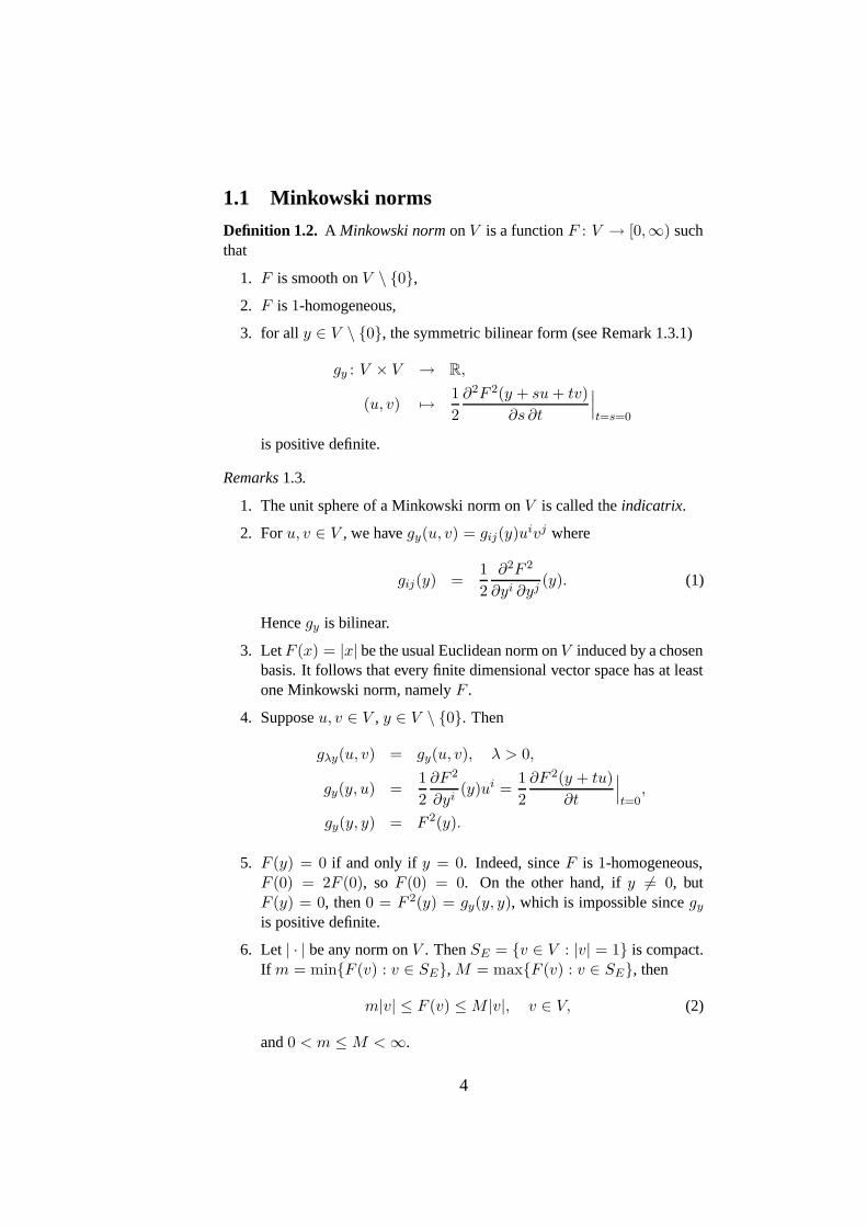
1.1 Minkowski norms

Definition 1.2. A Minkowski norm on V is a function F : V → [0,∞) suchthat

1. F is smooth on V \ 0,

2. F is 1-homogeneous,

3. for all y ∈ V \ 0, the symmetric bilinear form (see Remark 1.3.1)

gy : V × V → R,

(u, v) 7→1

2

∂2F 2(y + su + tv)

∂s ∂t

∣∣∣t=s=0

is positive definite.

Remarks 1.3.

1. The unit sphere of a Minkowski norm on V is called the indicatrix.

2. For u, v ∈ V , we have gy(u, v) = gij(y)uivj where

gij(y) =1

2

∂2F 2

∂yi ∂yj(y). (1)

Hence gy is bilinear.

3. Let F (x) = |x| be the usual Euclidean norm on V induced by a chosenbasis. It follows that every finite dimensional vector space has at leastone Minkowski norm, namely F .

4. Suppose u, v ∈ V , y ∈ V \ 0. Then

gλy(u, v) = gy(u, v), λ > 0,

gy(y, u) =1

2

∂F 2

∂yi(y)ui =

1

2

∂F 2(y + tu)

∂t

∣∣∣t=0

,

gy(y, y) = F 2(y).

5. F (y) = 0 if and only if y = 0. Indeed, since F is 1-homogeneous,F (0) = 2F (0), so F (0) = 0. On the other hand, if y 6= 0, butF (y) = 0, then 0 = F 2(y) = gy(y, y), which is impossible since gy

is positive definite.

6. Let | · | be any norm on V . Then SE = v ∈ V : |v| = 1 is compact.If m = minF (v) : v ∈ SE, M = maxF (v) : v ∈ SE, then

m|v| ≤ F (v) ≤ M |v|, v ∈ V, (2)

and 0 < m ≤ M < ∞.

4

7. F is continuous on V . Since F is differentiable on V \ 0, it isalso continuous there. That F is continuous at 0 follows by taking asequence converging to 0 and using the latter estimate in inequality(2).

8. B = v ∈ V : F (v) ≤ 1 is compact. This follows as B is closedand contained in the compact set v ∈ V : |v| ≤ 1/m.

9. Equation (2) implies that any two Finsler norms F , F on V are equiv-alent. That is, there are constants m,M > 0 such that

mF (v) ≤ F (v) ≤ MF (v), v ∈ V.

The next theorem shows that the unit ball B = v ∈ V : F (v) ≤ 1 isconvex. It also shows that if F is symmetric, then F is a norm in the usualsense.

Proposition 1.4 (Triangle inequality). [She01b] For v, w ∈ V , we have

F (v + w) ≤ F (v) + F (w)

with equality if and only if w = λv for some λ ≥ 0.

Proposition 1.5 (Cauchy-Schwarz inequality). [She01b] For v, y ∈ V ,y 6= 0, we have

gy(y, v) ≤ F (y)F (v),

with equality if and only if v = λy for some λ ≥ 0.

The proofs of the above two propositions are somewhat technical (seee.g. [She01b]) and are therefore omitted.

Proposition 1.6. [She01b] Suppose v, y ∈ V \ 0, and

gv(v, w) = gy(y, w)

for all w ∈ V . Then v = y.

Proof. Setting w = v and w = y yields

F 2(v) = gy(y, v) ≤ F (v)F (y),

F 2(y) = gv(v, y) ≤ F (v)F (y).

Thus F (y) = F (v), so

gv(v, y) = F (v)F (y),

and by the Cauchy-Schwarz inequality, v = y.

5

1.2 Legendre transformation

Definition 1.7 (Dual Minkowski norm). The dual Minkowski norm is thefunction F ∗ : V ∗ → R is defined as

F ∗(ξ) = maxξ(y) : y ∈ V, F (y) = 1, ξ ∈ V ∗.

As y ∈ V : F (y) = 1 is compact, the dual Minkowski norm is welldefined and finite. In what follows, we prove that a dual Minkowski normis a Minkowski norm on V ∗. For this purpose, we introduce the Legendretransformation.

Definition 1.8 (Legendre transformation). The Legendre transformation` : V → V ∗ is defined as `(y) = gy(y, ·) for y ∈ V \ 0, and `(0) = 0.

The first part of the next proposition gives an algebraic relation betweenF, F ∗ and `. The second part is essentially a variant of Riesz’ theorem.

Proposition 1.9.

1. F = F ∗ `.

2. The Legendre transformation is a bijection.

Proof. Property 1 is clear for y = 0, so suppose y 6= 0. Then

F (y) =gy(y, y)

F (y)= `y

(y

F (y)

)≤ F ∗ `(y),

and by the Cauchy-Schwarz inequality we have

F ∗ `(y) = supv 6=0

`y

(v

F (v)

)= sup

v 6=0

gy(y, v)

F (v)≤ F (y),

so property 1 holds. For property 2, let us first note that `(y) = 0 if andonly if y = 0. It therefore suffices to show that ` : V \ 0 → V ∗ \ 0 is abijection. Proposition 1.6 implies injectivity. To prove surjectivity, supposeξ ∈ V ∗ \ 0. Let λ = F ∗(ξ), and let y ∈ V be such that F (y) = 1 andξ(y) = λ. Now ξ(w) = 0, if

w ∈ Wy = w ∈ V : gy(y, w) = 0.

Indeed, if γ is the smooth curve γ : (−ε, ε) → F −1(1),

γ(t) =y + tw

F (y + tw), t ∈ (−ε, ε),

then as y is a stationary point of v 7→ ξ(v), we have

0 =d

dtξ(γ(t))

∣∣∣t=0

= ξ

(w

F (y)−

y

F 2(y)

∂F

∂yi(y)wi

),

6

and as gy(y, w) = 0, the second term vanishes and ξ(w) = 0. For any v ∈ Vwe have decomposition

v = w + gy(y, v)y, w = v − gy(y, v)y ∈ Wy.

This decomposition and ξ(w) = 0 for w ∈ Wy implies that ξ = `(λy).

Next we introduce some more notation. Let gij be the ij:th entry of theinverse matrix of (gij), let θi be the dual basis to ei, and let `i(y) be thei:th component of `(y),

`i(y) = `(y)(ei) =1

2

∂F 2

∂yi(y).

Proposition 1.10.

1. The dual Minkowski norm is a Minkowski norm on V ∗.

2. Let

g∗ij(ξ) =1

2

∂2F ∗2

∂ξi ∂ξj(ξ), ξ ∈ V ∗ \ 0. (3)

Then

`(y) = `j(y)θj = gij(y)yiθj, y ∈ V \ 0, (4)

`−1(ξ) = g∗ij(ξ)ξiej, ξ ∈ V ∗ \ 0, (5)

gij(y) = g∗ij `(y), y ∈ V \ 0. (6)

Proof. Let us first show that F ∗ is smooth on V ∗ \ 0. In view of Propo-sition 1.9.1, it suffices to prove that ` is a diffeomorphism ` : V \ 0 →V ∗ \ 0. By equation (4) (which is trivial), it follows that ` is smooth,and that the Jacobian of ` is (D`)ij = gij . Hence, by the inverse functiontheorem, the inverse of ` is smooth. It is evident that F ∗ is 1-homogeneous,so it remains to check the positive definite condition on F ∗. Differentiating12F 2 = 1

2F ∗2 ` with respect to yi and yj yields for y ∈ V \ 0,

1

2

∂F 2

∂yi(y) =

1

2

∂F ∗2

∂ξk `(y)gki(y), (7)

gij(y) = (g∗kl `)(y)gki(y)glj(y) +1

2

∂F ∗2

∂ξk `(y)

∂gki

∂yj(y). (8)

Equation (7) implies that `i(y) = (g∗kj `)(y)`j(y)gki(y), so

yj = g∗jk `(y)`k(y).

As gij is 0-homogeneous, we have

1

2

∂F ∗2

∂ξk `(y)

∂gki

∂yj(y) = (g∗km `)(y)`m(y)

∂gki

∂yj(y) = yk ∂gij

∂yk(y) = 0,

7

so the second term in equation (8) vanishes, and equation (6) follows. Letus recall that a matrix is positive definite if and only if all eigenvalues arepositive, and eigenvalues are transformed as µ 7→ 1/µ under matrix inver-sion. Therefore equation (6) implies that g∗ij is positive definite, and F ∗ isa Minkowski norm. Equation (5) follows since the mapping `−1 defined bythis equation satisfies `−1 ` = idV , and ` `−1 = idV ∗ .

8

2 Finsler geometry

By an n-dimensional manifold M we mean a topological Hausdorff spacewith countable base that is locally homeomorphic to Rn. In addition we as-sume that all transition functions are C∞-smooth. That is, we only considerC∞-smooth manifolds. The space of differential p-forms on M is denotedby ΩpM , and the tangent space of M is denoted by TM . By X (M) wedenote the set of vector fields on M . When we consider an object at somepoint x ∈ M , we use x as a sub-index on the object. For example, Ω1

xM isthe set of 1-forms originating from x. If f is a diffeomorphism, then by Dfwe mean the tangent map and by f ∗ the pullback of f .

Suppose (xi) are local coordinates around x ∈ M . Then we denote by∂

∂xi |x the standard basis vectors for TxM , and by dxi|x the standard basisvectors for T ∗

xM . When the base point x is clear from context, we simplywrite ∂

∂xi and dxi.

Definition 2.1 (Finsler manifold). A Finsler manifold is a manifold M anda function F : TM → [0,∞) (called a Finsler norm) such that

1. F is smooth on TM\0,

2. F |TxM : TxM → [0,∞) is a Minkowski norm for all x ∈ M .

Here TM\0 is the slashed tangent bundle, that is,

TM\0 =⋃

TxM \ 0 : x ∈ M.

Example 2.2. Let (M, g) be a Riemannian manifold. Then

F (x, y) =√

gx(y, y)

is a Finsler norm on M .

In addition to Finsler norms, we will also study co-Finsler norms. Theseform a special class of Hamiltonian functions.

Definition 2.3 (co-Finsler norm). A co-Finsler norm on a manifold M is afunction H : T ∗M → [0,∞) such that

1. H is smooth on T ∗M \ 0,

2. H|T ∗

x M : T ∗xM → [0,∞) is a Minkowski norm for all x ∈ M .

2.1 The global Legendre transforms

Next we generalize the pointwise Legendre transformations to a global trans-formation between TM and T ∗M . As a result we prove that Finsler andco-Finsler norms are in one-to-one correspondence.

9

The Legendre transform T∗M → TM

Suppose H is a co-Finsler norm on a manifold M . Then for each x ∈ Mwe have the pointwise Legendre transformation

`x : T ∗xM → T ∗∗

x M

induced by the Minkowski norm H|T ∗

x M , and the canonical linear isomor-phism

ι : TxM → T ∗∗x M.

Then we define the global Legendre transformation as

L : T ∗M → TM,

ξ 7→ ι−1 `π(ξ)(ξ),

where π : T ∗M → M is the canonical projection. It is clear that L is welldefined. In local coordinates, let

hij(ξ) =1

2

∂2H2

∂ξi ∂ξj(ξ), ξ ∈ T ∗M \ 0. (9)

Proposition 2.4. Suppose L is the Legendre transformation induced by aco-Finsler norm H .

1. L is a bijection T ∗M → TM and a diffeomorphism T ∗M \ 0 →TM \ 0.

2. F = H L −1 is a Finsler norm on M .

3. If gij is as in equation (1), and hij is the inverse of hij , then

L (ξ) = hij(ξ)ξi∂

∂xj, ξ ∈ T ∗M \ 0, (10)

L−1(y) = gij(y)yi dxj, y ∈ TM \ 0, (11)

gij(y) = hij L−1(y), y ∈ TM \ 0. (12)

Proof. Let us first prove equation (10) in part 3. For a fixed x ∈ M , letei be the usual basis ∂

∂xi induced by some local coordinates, and let θi,∆i be dual bases for T ∗

xM , T ∗∗x M , respectively. That is, θi, ∆i are

defined by conditions θi(ej) = δij and ∆i(θ

j) = δji , whence ι(ei) = ∆i,

ι−1(∆i) = ei, and θi = dxi. By equation (4),

L (ξ) = ι−1(hij(ξ)ξi∆j)

= hij(ξ)ξi∂

∂xj,

10

and equation (10) follows. For equation (11), let us first notice that if wi arecoordinates for T ∗∗

x M , then

gij(y) =1

2

∂2H2 `−1x

∂wi ∂wj(ι(y)),

so by equation (5),

L−1(y) = `−1

x ι(y)

=1

2

∂2H2 `−1x

∂wi ∂wj(ι(y))(ι y)iθj

= gij(y)yidxj ,

and equation (11) follows. Equation (12) follows using equations (6) and(13);

hij(ξ) =1

2

∂2H2 `−1x

∂wi ∂wj `x(ξ)

= gij L (ξ).

In part 1, it is clear that L is a bijection. Equation (10) shows that L issmooth on T ∗M \ 0, and since the Jacobian of L is of the form

DL =

(I 0∗ hij

),

part 1 follows by the inverse function theorem. For property 2, let us firstshow that F is 1-homogeneous. Suppose y ∈ TM . Then y = L (ξ) forsome ξ ∈ T ∗M , and as L is 1-homogeneous we have

L−1(λy) = L

−1(L (λξ)) = λξ = λL−1(y), λ > 0.

Since hij is positive definite, hij is positive definite, and gij is positive defi-nite by equation (12).

The Legendre transform TM → T∗M

Suppose F is a Finsler norm on a manifold M . For each x ∈ M , we canthen introduce a pointwise Legendre transformation

`x : TxM → T ∗xM

induced by the Minkowski norm F |TxM . Then we define the global Legen-dre transformation as

L : TM → T ∗M,

y 7→ `π(y)(y),

where π : TM → M is the canonical projection.

11

Proposition 2.5. Suppose L is the Legendre transformation induced by aFinsler norm F .

1. L is a bijection TM → T ∗M and a diffeomorphism TM \ 0 →T ∗M \ 0.

2. H = F L −1 is a co-Finsler norm.

3. If gij be as in equation (1), hij be as in equation (9), and is hij be theinverse of hij , then

L (y) = gij(y)yi dxj , y ∈ TM \ 0, (13)

L−1(ξ) = hij(ξ)ξi

∂

∂xj, ξ ∈ T ∗M \ 0, (14)

hij(ξ) = gij L−1(ξ), ξ ∈ T ∗M \ 0. (15)

Proof. The proof is completely analogous to the proof of Proposition 2.4,but much simpler since there is no ι mapping.

Example 2.6 (Musical isomorphisms). Suppose (M, g) is a Riemannian man-ifold. Then F (y) =

√g(y, y) makes M into a Finsler manifold. The in-

duced Legendre transformation acts on vectors and co-vectors as follows:

L (y) = gij(x)yidxj , y ∈ TxM,

L−1(ξ) = gij(x)ξi

∂

∂xj, y ∈ TxM.

Here we use standard notation: gij(x) = g( ∂∂xi

∣∣x, ∂

∂xj

∣∣x), and gij(x) is

the inverse of (gij). From the above formulas, we see that in this specialcase, the Legendre transformation reduces to the musical isomorphisms inRiemannian geometry; L (y) = y[, and L −1(ξ) = ξ].

The next two results show that the Legendre transformations are in somesense well behaved.

Proposition 2.7. Suppose LH is the Legendre transformation induced by aco-Finsler norm H , and LF is the Legendre transformation induced by theFinsler norm F = H L

−1H . Then

LF = L−1H . (16)

Similarly, if LF is the Legendre transformation induced by a Finsler normF , and LH is the Legendre transformation induced by the co-Finsler normH = F L

−1F , then equation (16) also holds.

Proof. Both claims follow using equations (11) and (13).

Corollary 2.8. On a fixed manifold, Finsler and co-Finsler norms are inone-to-one correspondence via the two Legendre transformations.

12

Proof. Let T be mapping F 7→ F L−1F that maps a Finsler norm F to a co-

Finsler norm, and let S be mapping H 7→ H L−1H that maps a co-Finsler

norm H to a Finsler norm. If H is a co-Finsler norm, then

T S(H) = T (F ) = F L−1F = H L

−1H L

−1F = H

where F = H L−1H , and similarly, S T = id.

13

14

3 Geodesics

Suppose M is a manifold. Then a curve is a smooth mapping c : (a, b) → Msuch that (Dc)t 6= 0 for all t. Such a curve has a canonical lift c : (a, b) →TM \ 0 defined as c(t) = (Dc)(t), where Dc is the tangent of c. If,furthermore, M is a Finsler manifold with Finsler norm F , we define thelength of c as

L(c) =

∫ b

aF c(t) dt,

and the energy as

E(c) =1

2

∫ b

aF 2 c(t) dt.

A curve c that satisfies F c = 1 is called path-length parameterized.The next proposition shows that every curve can be path-length parametrized,and the length of an oriented curve does not depend on its parametrization.The latter claim need not be true for the energy.

Proposition 3.1. Suppose c is a curve on a Finsler manifold (M,F ).

1. If α : (a′, b′) → (a, b) is a diffeomorphism with α′ > 0, then c α =α′c α, and L(c α) = L(c).

2. There is a diffeomorphism α : (0, L(c)) → (a, b) such that

F c α = 1. (17)

Proof. The first claim follows since F is 1-homogeneous. For the secondclaim, let us define β : (a, b) → (0, L(c)) by

β(s) =

∫ s

aF c(t) dt.

Then β′(s) = F c(s) > 0, so by the inverse function theorem, β is smoothand invertible with smooth inverse. The sought diffeomorphism is α = β−1;

F c α = F ((β−1)′c α)

=1

β′ β−1F c α

= 1.

Definition 3.2 (Variation). Suppose c : (a, b) → M is a curve. Then avariation of c is a continuous mapping H : [a, b] × (−ε, ε) → M for someε > 0 such that

1. H is smooth on (−ε, ε) × (a, b),

15

and with notation cs(·) = H(·, s),

2. c0(t) = c(t), for all t ∈ [a, b],

3. cs(a), cs(b) ∈ M are constants not depending on s ∈ (−ε, ε).

Definition 3.3 (Geodesic). A curve c in a Finsler manifold is a geodesic ifL is stationary at c, that is, for any variation (cs) of c,

d

dsL(cs)

∣∣∣s=0

= 0.

Our next aim is to prove Proposition 3.6 which gives a local condition fora curve to be a geodesic. To do this, we need to operate with vectors on TM ,that is, with elements in T (TM). Let us therefore start by deriving theirtransformation properties. First, if (xi) and xi = xi(x) are local coordinatesaround some x ∈ M , then

∂

∂xi

∣∣∣x

=∂xj

∂xi

∂

∂xj

∣∣∣x. (18)

Here ∂xj

∂xi is the Jacobian of the mapping taking (xi)-coordinates into (xi)-coordinates evaluated at the local xi-coordinates for x.

Next, suppose (xi, yi), (xi, yi) are standard local coordinates around y ∈TxM . That is, xi = xi(x), yi = yi(x, y), and yi are coordinates in the ∂

∂xi

basis. It follows that vectors

∂

∂xi

∣∣∣y,

∂

∂yi

∣∣∣y,

∂

∂xi

∣∣∣y,

∂

∂yi

∣∣∣y∈ T (TM \ 0)

satisfy transformation rules

∂

∂xi

∣∣∣y

=∂xr

∂xi

∂

∂xr

∣∣∣y

+∂2xr

∂xi ∂xsys ∂

∂yr

∣∣∣y, (19)

∂

∂yi

∣∣∣y

=∂xr

∂xi

∂

∂yr

∣∣∣y. (20)

In fact, equation (18) implies that yi = ∂xi

∂xr yr, so

∂

∂xi

∣∣∣y

=∂xr

∂xi

∂

∂xr

∣∣∣y

+∂yr

∂xi

∂

∂yr

∣∣∣y,

and equation (19) follows. The proof of equation (20) is similar.

Lemma 3.4 (Euler equations). Suppose f : TM \ 0 → R is a smoothfunction. Then a smooth curve c : (a, b) → M is stationary for c 7→

∫ ba f

c(t) dt if and only if for each t there are local coordinates around c(t) suchthat

∂f

∂xi c −

d

dt

(∂f

∂yi c

)= 0. (21)

Moreover, condition (21) does not depend on local coordinates.

16

Proof. The last claim follows from equations (19) and (20). Before theproof, let us begin with an observation. Suppose c is a curve, and a = t1 <· · · < tN = b is a partition of the domain of c such that each (ti, ti+1) ismapped into one coordinate chart. Furthermore, suppose H(t, s) = cs(t) isa variation of c and by restricting the value of s, we can assume that eachpartition (ti, ti+1) is mapped into one coordinate chart by H . If K is themapping c 7→

∫ ba f c(t) dt, then

d

dsK(cs)

∣∣∣s=0

=N−1∑

k=1

∫ tk+1

tk

[∂f

∂xi c(t)

∂Hi

∂s(t, 0) +

∂f

∂yi c(t)

∂2Hi

∂t ∂s(t, 0)

]dt

=

N−1∑

k=1

∫ tk+1

tk

[∂f

∂xi c(t) −

d

dt

(∂f

∂yi c(t)

)]∂Hi

∂s(t, 0) dt.

For the actual proof, suppose that c : (a, b) → M is a stationary curve. Thenrestrictions of c to subsets of (a, b) are also stationary, so we can assume thatc is contained in one coordinate chart, and the claim follows from the abovecalculation. On the other hand, if condition (21) holds, then c is stationarysince equation (21) is independent of local coordinates.

One can prove that a stationary curve is smooth if it is piecewise smooth[She01b]. Intuitively, this is easy to understand; if a geodesic has a kink, itcan be shortened by smoothing.

Definition 3.5 (Geodesic coefficients). In a Finsler manifold, the geodesiccoefficients are locally defined functions

Gi(y) =1

4gik(y)

(2∂gjk

∂xl−

∂gjl

∂xk

)yjyl, y ∈ TM \ 0. (22)

Proposition 3.6 (Geodesic equation). A curve c : I → M is stationary forE if and only if for each t ∈ I there are local coordinates such that

d2ci

dt2+ 2Gi c = 0.

Proof. This follows by Lemma 3.4, relations F 2(y) = gij(y)yiyj , ∂F 2

∂yi (y) =

2gijyj , and Euler’s theorem.

Definition 3.7 (Geodesic spray). Geodesic spray G ∈ X (TM \ 0) on aFinsler manifold is locally defined as

G|y = yi ∂

∂xi

∣∣∣y− 2Gi(y)

∂

∂yi

∣∣∣y. (23)

17

In Proposition 7.14 we prove that G is well defined, that is, G does notdepend on local coordinates. Without any circular argument, let us assumethis to be known. (Alternatively, one can prove this by a very long calcu-lation, but there is no need to do that here.) It follows that Gi satisfy thetransformation rule

Gr =∂xr

∂xiGi −

1

2

∂2xr

∂xi ∂xsyiys. (24)

The next proposition is a coordinate independent restatement of Propo-sition 3.6.

Proposition 3.8. Suppose π is the canonical projection π : TM → M . If cis an integral curve of G, then πc is a stationary curve of E, and c = π c.Conversely, if b is a stationary curve for E, then b is an integral curve of G.

It turns out that stationary curves of E and L almost coincide. The firsthalf of this equivalence is contained in the proposition below. After weintroduce some tools from symplectic geometry we also prove the converse(Proposition 7.16); every stationary curve of E is a geodesic. In view ofthis equivalence, it will be convenient to consider only stationary points ofE. Traditionally this is done for two reasons. First, it gives slightly simplerformulas. For example, compare derivatives of F =

√gij(x)yiyj and F 2 =

gij(x)yiyj , and second, stationary curves of E naturally generalize also tothe case when F is non-degenerate (which is not relevant here).

Proposition 3.9. If c is a geodesic, and α is a diffeomorphism such that cαis parameterized with respect to pathlength, then c α is a stationary pointof E.

Proof. Using Lemma 3.4 and the 1-homogeneity of F , it follows that cα isa stationary curve for L. By writing derivatives as ∂F

∂xi = 12F

∂F 2

∂xi and usingLemma 3.4 again the result follows.

18

4 Horizontal and vertical decompositions

In many respects, Finsler geometry is analogous to Riemann geometry. How-ever, a typical difference is that in Finsler geometry objects exist on TMwhereas in Riemann geometry they exist on M . For example, in Finslergeometry, curvature is a tensor on TM \ 0, whereas in Riemannian ge-ometry, it is a tensor on M . For this reason we need to study vectors andco-vectors on TM , that is, elements in T (TM \ 0) and T ∗(TM \ 0).Equations (19)-(20) already give the transformation rules for basis vectorsin T (TM \ 0). In this section we define the horizontal–vertical decom-position in T (TM \ 0) and T ∗(TM \ 0). This decomposition willgreatly simplify calculations in local coordinates. It will also give a certainstructure compatible with the Finsler metric. For example, the tangent ofa geodesic will be a horizontal vector. Also, the derivative of F will be avertical co-vector. Some immediate applications of the horizontal–verticaldecomposition are given in Section 4.1.

In order to introduce the horizontal–vertical decomposition, one needs anon-linear connection, that is, one needs some structure on TM \ 0.

Definition 4.1 (Non-linear connection). A non-linear connection on a man-ifold M is a collection of locally defined 1-homogeneous functions N i

j onTM \ 0 satisfying transformation rules

∂xj

∂xiNh

j =∂xh

∂xjN j

i −∂2xh

∂xi ∂xjyj.

Let Gi be the coefficients for the geodesic spray, and let

N ij =

∂Gi

∂yj. (25)

Then N ij are 1-homogeneous, and by differentiating equation (24) we see

that N ij are coefficients for a non-linear connection. It is the only non-linear

connection we shall use in this work. However, let us emphasize that onecan study non-linear connections also without Finsler geometry. Conceptssuch as covariant derivative, geodesics, and curvature can all be defined fromonly a non-linear connection [MA94].

Decomposition of T (TM \ 0)

Equation (19) shows that the vector subspace span ∂∂xi |y : i = 1, . . . , n

depends on local coordinates. Therefore one can not talk about “ ∂∂xi ”-

directions in T (TM \0). However, when M is equipped with a non-linearconnection N i

j , let

δ

δxi

∣∣∣y

=∂

∂xi

∣∣∣y− Nk

i (y)∂

∂yk

∣∣∣y∈ T (TM \ 0),

19

whenceδ

δxi

∣∣∣y

=∂xr

∂xi

δ

δxr

∣∣∣y.

Thus, the 2n-dimensional vector space Ty(TM\0) has two n-dimensionalsubspaces,

VyTM = span

∂

∂yi

∣∣∣y

, HyTM = span

δ

δxi

∣∣∣y

,

and these are independent of local coordinates. Let us also define

V TM =⋃

y∈TM\0

VyTM, H TM =⋃

y∈TM\0

HyTM,

whence pointwise

T (TM \ 0) = V TM ⊕ H TM.

Vectors in V TM are called vertical vectors, and vectors in H TM arecalled horizontal vectors.

The next example shows that the tangent of a geodesics is always a hor-izontal vector. Thus, in some sense, horizontal vectors are more importantthan vertical vectors. This also motivates that name; one can move horizon-tally, but not vertically.

Example 4.2. The coefficients Gi for the geodesic spray are 2-homogeneous.Hence 2Gi = yj ∂Gi

∂yj = yjN ij , so

G = yi δ

δxi,

and G(y) is horizontal for all y ∈ TM \ 0.

Decomposition of T∗(TM \ 0)

On TM , the 1-forms dxi and dyi satisfy

dxi∣∣y

=∂xi

∂xrdxr

∣∣y, (26)

dyi∣∣y

=∂xi

∂xrdyr

∣∣y

+∂2xi

∂xr ∂xsyrdxs

∣∣y. (27)

These transformation rules follow from transformation rules (19)-(20) andthe following lemma:

Lemma 4.3. Suppose ai, ai are bases for a finite dimensional vectorspace V . Furthermore, suppose that αi, and αi are correspondingdual bases. Say, αi is defined by conditions: αi : V → R is linear, andαi(aj) = δi

j . Then

αj =∑

m

αj(am)αm.

20

Proof. If αj =∑

m Λjmαm, then αj(am) = Λj

m.

Let

δyi|y = dyi|y + N ij(y)dxj |y,

whence

δyi|y =∂xi

∂xrδyr|y.

Thus the 2n-dimensional vector space T ∗y (TM\0) has two n-dimensional

subspaces,

V∗

y TM = spanδyi|y

, H

∗y TM = span

dxi|y

,

and these are independent of local coordinates. Then pointwise

T ∗(TM \ 0) = V∗TM ⊕ H

∗TM.

Co-vectors in V ∗TM are called vertical covectors, and co-vectors in H ∗TMare called horizontal covectors.

Proposition 4.4. Suppose δδxi , ∂

∂yi , dxi, and δyi are defined via the non-linear connection (25). Then

dxi

(δ

δxj

)= δi

j , dxi

(∂

∂yj

)= 0,

δyi

(δ

δxj

)= 0, δyi

(∂

∂yj

)= δi

j , (28)

[δ

δxj,

δ

δxk

]=

(δNm

j

δxk−

δNmk

δxj

)∂

∂ym,

[δ

δxi,

∂

∂yj

]=

[δ

δxj,

∂

∂yi

]=

∂Nkj

∂yi

∂

∂yk, (29)

[∂

∂yi,

∂

∂yj

]= 0.

Proof. The last three equations follow from the definition of the Lie bracket;if X,Y are vector fields, then [X,Y ] is the vector field such that [X,Y ](f) =X(Y (f)) − Y (X(f)). The first equality in equation (29) follows since

∂N ij

∂yk=

∂N ik

∂yj.

Proposition 4.5. If f : TM \ 0 → R is a smooth function, then

df =δf

δxidxi +

∂f

∂yiδyi.

21

4.1 Applications

Suppose M is a manifold with a Finsler metric F . Then two immediateapplications of the horizontal–vertical decomposition are the Sasaki metricand the almost complex structure for T (TM \ 0).

Sasaki metric

Letg = gij(y)dxi ⊗ dxj + gij(y)δyi ⊗ δyj .

Then g is a Riemannian metric on TM \ 0 known as the Sasaki metric.The Legendre transformation induced by g,

[ : T (TM \ 0) → T ∗(TM \ 0)

is given by

[

(δ

δxi

)= gikdxk, [

(∂

∂yi

)= gikδy

k.

Another Riemannian metrics on TM \ 0 is the Cheeger-Gromoll met-ric. For both of these metrics, one can derive explicit expressions for thecovariant derivative and curvature. For example, see [Kap01].

Almost complex structure

Suppose E is a even dimensional manifold, and J : TE → TE is a linearmap in each tangent space. Then J is an almost complex structure if J 2 =− Id [MS97].

Using the horizontal–vertical decomposition we can define an almostcomplex structure J : T (TM \ 0) → T (TM \ 0) by setting

J

(δ

δxi

)=

∂

∂yi, J

(∂

∂yi

)= −

δ

δxi. (30)

Then J2 = − Id, and J does not depend on the local coordinates appearingin the definition. The map J is compatible with the Sasaki metric. That is

g(X,Y ) = g(JX, JY ), X, Y ∈ T (TM \ 0).

The Nijenhuis tensor associated with an almost complex structure J isdefined by

N(X,Y ) = [JX, JY ] − J [JX, Y ] − J [X, JY ] − [X,Y ]

for vector fields X,Y .

Proposition 4.6. Every Nijenhuis tensor N satisfies properties:

22

1. N is bilinear over smooth functions.

2. N is anti-symmetric.

3. N(X, JX) = 0 for any vector field X .

Proof. If f, g are functions and X,Y are vector fields, then the Lie bracketsatisfies

[fX, gY ] = fX(g)Y − gY (f)X + fg[X,Y ].

Using this identity, it follows that

N(fX, gY ) = fgN(X,Y ),

and the first property follows. The latter two properties are immediate.

Proposition 4.7. The Nijenhuis tensor for the almost complex structure (30)is given by

N

(δ

δxi,

δ

δxj

)= −

[δ

δxi,

δ

δxj

],

N

(δ

δxi,

∂

∂yj

)= J

[δ

δxi,

δ

δxj

],

N

(∂

∂yi,

∂

∂yj

)=

[δ

δxi,

δ

δxj

].

The Newlander-Nirenberg theorem states that an almost complex struc-ture is integrable (see [MS97]) if and only if the Nijenhuis tensor vanishesidentically. Thus, for the almost complex structure J : T (TM \ 0) →T (TM \ 0), this is the case if

[δ

δxi ,δ

δxj

]= 0 identically for all i, j. In

Section 6 we will see that this is equivalent to the curvature being zero.

23

24

5 Finsler connections

5.1 Finsler connections

Definition 5.1 (Finsler connection). A Finsler connection is determinedby a triple (N,F,C) where N is a non-linear connection on M and F =(F i

jk), C = (C ijk) are collections of locally defined 0-homogeneous func-

tions F ijk, C

ijk : TM \ 0 → R satisfying the transformation rules

∂xl

∂xiF i

jk =∂2xl

∂xj ∂xk+

∂xr

∂xj

∂xs

∂xkF l

rs, (31)

Cijk =

∂xi

∂xp

∂xq

∂xj

∂xr

∂xkCp

qr. (32)

Suppose π : TM → M is the canonical projection. The Finsler connection(induced by (N,F,C)) is the mapping

∇ : Ty(TM \ 0) × X (M) → Tπ(y)(M), (Y,X) 7→ ∇Y (X)

defined by the properties

1. ∇ is linear over R in X and Y (but not necessarily in y),

2. If f ∈ C∞(M) and y ∈ TxM \ 0, then in local coordinates

∇ δ

δxi |y(f

∂

∂xj

∣∣∣x) = df(

∂

∂xi

∣∣∣x)

∂

∂xj

∣∣∣x

+ fF mij (y)

∂

∂xm

∣∣∣x,

∇ ∂

∂yi |y(f

∂

∂xj

∣∣∣x) = fCm

ij (y)∂

∂xm

∣∣∣x.

From the transformation properties of F ijk and C i

jk it follows that

∇ δ

δxi(X) =

∂xr

∂xi∇ δ

δxr(X),

∇ ∂

∂yi(X) =

∂xr

∂xi∇ ∂

∂yr(X),

for all X ∈ X (M), so ∇ does not depend on the local coordinates.Below are four examples of Finsler connections [Ana96]. Of these, the

Berwald connection depends only on a non-linear connection. All the otherconnections depend on the Finsler norm. Thus, a non-linear connection de-fines a non-linear covariant derivative and a linear Finsler connection.

Chern-Rund connection

Let (M,F ) be a Finsler manifold, and let

Γijk =1

2

(δgik

δxj+

δgij

δxk−

δgjk

δxi

),

Γijk = girΓrjk,

25

be locally defined functions. Then (N ij ,Γ

ijk, 0) is the Chern-Rund connec-

tion.That Γi

jk satisfies the appropriate transformation rule follows from

Γijk =∂xp

∂xi

(∂2xq

∂xj ∂xkgpq +

∂xq

∂xj

∂xr

∂xkΓpqr

), (33)

gij =∂xi

∂xr

∂xj

∂xsgrs. (34)

The latter transformation rule follows from

gij =∂xr

∂xi

∂xs

∂xjgrs. (35)

Berwald connection

Let Gijk =

∂N ij

∂yk , where N ij are given by equation 25. Then (N i

j , Gijk, 0) is

the Berwald connection.

Hashiguchi connection

On a Finsler manifold the Cartan tensor Cijk is defined as

Cijk =1

2

∂gij

∂yk=

1

4

∂3F 2

∂yi ∂yj ∂yk,

C ljk = gliCijk.

Coefficients C ijk satisfy equation (32), and the connection (N i

j , Gijk, C

ijk) is

the Hashiguchi connection.

Cartan connection

The Cartan connection is the Finsler connection (N ij ,Γ

ijk, C

ijk).

5.2 Covariant derivative

Definition 5.2 (Covariant derivative). Suppose M is a manifold with anon-linear connection N i

j . Then the covariant derivative (induced by N ij ) is

a mapping

D : TxM \ 0 × X (M) → TxM \ 0, (y,X) 7→ Dy(X)

determined by the following properties:

1. Dy(X + Y ) = Dy(X) + Dy(Y ) for all X,Y ∈ X (M) and y ∈TM \ 0,

26

2. Dy(fX) = df(y)X + fDy(X) for all X ∈ X (M) and f ∈ C∞(M),

3. in local coordinates, Dy(∂

∂xi

∣∣x) = N j

i (y) ∂∂xj

∣∣x

for all y ∈ TxM \0.

Using the transformation rule for N ij , it follows that

Dy(∂

∂xi

∣∣x) =

∂xj

∂xiDy(

∂

∂xj) + d(

∂xh

∂xi)(y)

∂

∂xh

∣∣∣x

and Dy is well defined. In general, Dy(X) does not need to be linear in thelower argument. This is why N i

j called a non-linear connection.

5.3 Some properties of basic Finsler quantities

Let L : T ∗M → TM be the Legendre transformation induced by a co-Finsler metric h. In local coordinates, let L (ξ) = L i(ξ) ∂

∂xi and L −1(y) =

L−1i (y)dxi for ξ ∈ T ∗M and y ∈ TM , whence

Li(ξ) = hij(ξ)ξj , ξ ∈ T ∗M,

L−1i (y) = gij(y)yj , y ∈ TM.

Properties of Γ

Let Cijkl =∂Cijk

∂yl . Furthermore, let us define Lijk as

Lijk =∂Cijk

∂xsys − 2CijksG

s − N si Csjk − N s

j Csik − N skCsij.

These are components determining the Landsberg tensor [She01b]. Thefunctions Lijk are symmetric in the indices i, j, k; exchanging any two in-dices of i, j, k does not change Lijk. Also, as Cijky

k = 0, and Cijklyl =

−Cijk, it follows that

Lijkyi = Ljiky

i = Ljkiyi = 0. (36)

Lemma 5.3 (Properties of Chern-Rund connection).

Γijk = gimGmjk − Lijk (37)

Γijk = Γikj (38)

Γijky

j = N ik (39)

ΓijkL

−1i = Gi

jkL−1i = Γijky

i (40)

Proof. Let first us prove equation (37). From the definition of Γijk it followsthat

Γijk = γijk − N sj Csik − N s

kCsij + N si Csjk

27

where

γijk =1

2

(∂gik

∂xj+

∂gij

∂xk−

∂gjk

∂xi

).

Differentiating the expression for gisGs (see equation (22)) with respect to

yj and yk and using the identity ∂Cijk

∂yr yi = 0 gives

gisGsjk = γijk +

∂Cijk

∂xsys − 2CijksG

s − 2N sj Csik − 2N s

kCsij,

and equation (37) follows. The other equations follow from equations (36)and (37).

Lemma 5.4 (Derivatives of gij , hij).

∂L−1j

∂xk=

∂gij

∂xkyi = gjsN

sk + Γijky

i (41)

∂L j

∂xk=

∂hij

∂xkξi =

(∂gij

∂xkL

−1i

) L =

(−N j

k − gjsΓrskyr) L(42)

∂h2

∂xk=

∂hij

∂xkξiξj =

(∂gij

∂xkL

−1i L

−1j

) L =

(−2N r

kL−1r

) L(43)

Proof. Equation (41) follows from δgij

δxk = Γijk + Γjik and equation (39).The second equality in equation (42) follows since hij = gij L , and

∂gij

∂yrL

−1j =

∂gij

∂yrgjsy

s

= −gij ∂gjs

∂yrys

= 0.

The third equality in equation (42) follows by a similar calculation for ∂gij

∂xr L−1j .

Equality (43) follows from equations (42), (39), and (40).

28

6 Curvature

In Riemann geometry, the Riemann curvature tensor is a tensor on M . Wenext derive an analogous curvature tensor in a Finsler setting, which will bea tensor on TM \ 0.

Let us first note that[

δ

δxj,

δ

δxk

]= −

(δNm

k

δxj−

δNmj

δxk

)∂

∂ym.

where [·, ·] is the Lie bracket for vector fields. Let us define

Rmjk =

δNmk

δxj−

δNmj

δxk.

Proposition 6.1 (Mo). [She01a] H (M) is a submanifold near y ∈ TM \0 if and only if all the Rm

ij -symbols vanish in a neighbourhood of y.

Proof. This follows from a standard result about commuting vector fields.See for example [Con93], p. 110.

In addition to Rmij , let us furthermore define

Rmijk =

∂Rmjk

∂yi,

and the curvature tensor R, as

R = Rmijkdxi ⊗ dxj ⊗ dxk ⊗

δ

δxm.

To see that R is a tensor, let us first note that on TM , the 1-forms dxi anddyi satisfy

dxi∣∣y

=∂xi

∂xrdxr

∣∣y,

dyi∣∣y

=∂xi

∂xrdyr

∣∣y

+∂2xi

∂xr ∂xsyrdxs

∣∣y.

(Actually, similarly as on the tangent bundle, one can also define horizontaland vertical 1-forms on TM \ 0, but we shall not need these. See forexample [She01b, She01a].) Secondly, on overlapping coordinates,

[δ

δxi,

δ

δxj

]=

∂xr

∂xi

∂xs

∂xj

[δ

δxr,

δ

δxs

],

so Rmij = ∂xr

∂xi∂xs

∂xj∂xm

∂xn Rnrs and R is well defined.

29

Lemma 6.2. The 0-homogeneous functions Rmijk satisfy

0 = Rmijk + Rm

jki + Rmkij , (44)

Rmijk = −Rm

ikj, (45)

Rmijk =

δGmik

δxj−

δGmij

δxk+ Gs

ikGmjs − Gs

ijGmks. (46)

Proof. Equation (45) follows from the definition, equation (46) follows from

Rmjk =

∂Nmk

∂xj− N s

j Gmsk −

(∂Nm

j

∂xk− N s

kGmsj

),

and equation (44) follows from equation (46).

30

7 Symplectic geometry

Next we show that T ∗M \0 and TM \0 are symplectic manifolds, andstudy geodesics and the Legendre transformation in this symplectic setting.

Definition 7.1. Suppose ω is a 2-form on a manifold M . Then ω is non-degenerate, if for each x ∈ M , we have the implication: If a ∈ TxM , andωx(a, b) = 0 for all b ∈ TxM , then a = 0.

Definition 7.2 (Symplectic manifold). Let M be an even dimensional man-ifold, and let ω be a closed non-degenerate 2-form on M . Then (M,ω) is asymplectic manifold, and ω is a symplectic form for M .

Definition 7.3 (Hamiltonian vector field). Suppose (M,ω) is a symplecticmanifold, and suppose H be a function H : M → R. Then the Hamiltonianvector field induced by H is the unique (see next paragraph) vector fieldXH ∈ X (M) determined by the condition dH = ιXH

ω.

In the above, ι is the contraction mapping ιX : ΩrM → Ωr−1M definedby (ιXω)(·) = ω(X, ·). To see that XH is well defined, let us considerthe mapping X 7→ ω(X, ·). By non-degeneracy, it is injective, and by therank-nullity theorem, it is surjective, so the Hamiltonian vector field XH isuniquely determined.

Proposition 7.4 (Conservation of energy). Suppose (M,ω) is a symplecticmanifold, XH is the Hamiltonian vector field XH ∈ X (M) correspondingto a function H : M → R, and c : I → M is an integral curve of XH . Then

H c = constant.

Proof. Let t ∈ I . Since c is an integral curve, we have (Dc)(t, 1) = (XH c)(t), so for τ = (t, 1) ∈ TtI , we have

d(H c)t(τ) = (c∗dH)t(τ)

= (dH)c(t)

((Dc)(τ)

)

= (dH)c(t)

((XH c)(t)

)

= 0,

since ω is antisymmetric. The claim follows since d(H c) is linear.

Definition 7.5 (Symplectic mapping). Suppose (M,ω) and (N, η) are sym-plectic manifolds of the same dimension, and f is a diffeomorphism Φ: M →N . Then Φ is a symplectic mapping if Φ∗η = ω.

Proposition 7.6. Suppose (M,ω) is a symplectic manifold, and XH is aHamiltonian vector field corresponding to a function H : M → R. Further-more, suppose Φ: I ×U → M is the local flow of XH defined in some open

31

U ⊂ M and open interval I containing 0. Then for all x ∈ U , t ∈ I , wehave

(Φ∗t ω)x = ωx,

where Φt = Φ(t, ·).

Proof. As Φ0 = idM , we know that the relation holds, when t = 0. There-fore, let us fix x ∈ U , a, b ∈ TxM , and consider the function r(t) =(Φ∗

t ω)x(a, b) with t ∈ I . Then

r′(t) =d

ds

[r(s + t)

]∣∣∣s=0

=d

ds

[(Φ∗

sω)y(a′, b′)

]∣∣∣s=0

=(LXH

ω)y(a′, b′),

where y = Φt(x), a′ = (DΦt)(a), b′ = (DΦt)(b), and the last line is thedefinition of the Lie derivative. Using Cartan’s formula, LX = ιX d + d ιX , we have

LXHω = ιXH

dω + dιXHω

= ιXH0 + ddH

= 0,

so r′(t) = 0, and r(t) = r(0) = ωx(a, b).

Suppose M,N are manifolds, Ψ: M → N is a diffeomorphism. Thenthe pullback of Ψ for vector fields is the mapping

Ψ∗ : X (N) → X (M) ,

Y 7→ (DΨ−1) Y Ψ.

Proposition 7.7. Suppose (M,ω), (N, η) are symplectic manifolds, Φ: M →N is a symplectic mapping such that Φ∗η = ω, and h : N → R is a smoothfunction. Then

Φ∗(Xh) = XhΦ.

What is more, if c : I → N is an integral curve of Xh ∈ X (N), then Φ−1 cis an integral curve of XhΦ.

Proof. The contraction operator satisfies

ιΦ∗X(Φ∗η) = Φ∗(ιXη)

for all η ∈ Ωk(N), X ∈ X (N). Thus,

ιΦ∗Xhω = Φ∗(ιXh

η)

= Φ∗(dh)

= d(h Φ)

= ιXhΦω,

32

and as ω is non-degenerate, Φ∗Xh = XhΦ. In consequence,

D(Φ−1 c) = DΦ−1 Xh c = (Φ∗Xh)(Φ−1 c) = XhΦ(Φ−1 c),

so Φ−1 c is an integral curve of XhΦ.

7.1 Symplectic structure on T∗M \ 0

For any manifold its cotangent bundle is a symplectic manifold.

Definition 7.8 (Poincare 1-form). Suppose M is an manifold. Then thePoincare 1-form θ ∈ Ω1

(T ∗M \ 0

)is defined as

θ = −ξidxi.

where (xi, ξi) are local coordinates for T ∗M \ 0.

If (xi, ξi) are other standard coordinates for T ∗M \0, then ξi = ∂xr

∂xi ξr,

and ξidxi = ∂xr

∂xi ξr∂xi

∂xl dxl = ξidxi. Hence θ is well defined.

Lemma 7.9 (Coordinate independent expression for θ). Let π be the can-onical projection π : T ∗M → M . Then the Poincare 1-form θ ∈ Ω1(T ∗M)satisfies

θξ(v) = ξ((Dπ)(v)

)

for ξ ∈ T ∗Q and v ∈ Tξ

(T ∗Q

).

Proof. Let (xi, yi) be standard coordinates for T ∗Q near ξ. Then we canwrite ξ = ξidxi|π(ξ) and v = αi ∂

∂xi |ξ+βi ∂∂yi

|ξ , Thus (Dπ)(v) = αi ∂∂xi |π(ξ),

and θξ(v) = yi(ξ)dxi|ξ(v) = ξiαi = ξ

((Dπ)(α)

).

Proposition 7.10. The cotangent bundle T ∗M \ 0 of manifold M is asymplectic manifold with a symplectic form ω given by

ω = dθ = dxi ∧ dξi,

where θ is the Poincare 1-form θ ∈ Ω1(T ∗M \ 0

).

Proof. It is clear that ω is closed. If X = ai ∂∂xi + bi ∂

∂ξi, and Y = vi ∂

∂xi +

wi ∂∂ξi

, then ω(X,Y ) = a ·w− b · v. By setting v = w we obtain a = b, andby setting w = 0 we obtain a = b = 0.

The next example shows that we can always formulate Hamilton’s equa-tions on the cotangent bundle. This motivates the name for XH .

33

Example 7.11 (Hamilton’s equations). Suppose M is a manifold, H is afunction T ∗M → R, and XH ∈ X (T ∗M \ 0) is the correspondingHamiltonian vector field. If (xi, ξi) are standard coordinates for T ∗M \0,then

XH =∂H

∂ξi

∂

∂xi−

∂H

∂xi

∂

∂ξi.

Suppose that γ : I → T ∗M \ 0 is an integral curve to XH and locallyγ = (c, p). Then

dci

dt=

∂H

∂ξi γ,

dpi

dt= −

∂H

∂xi γ,

that is, integral curves of XH are solutions to Hamilton’s equations in localcoordinates of T ∗M .

7.2 Symplectic structure on TM \ 0

The previous section shows that T ∗M \ 0 is always a symplectic mani-fold. No such canonical symplectic structure is known for the tangent bun-dle. However, if M is a Finsler manifold, then TM \ 0 has a canonicalsymplectic structure induced by the Hilbert 1-form on TM \ 0.

Definition 7.12 (Hilbert 1-form). Let F be a Finsler norm on M . Then theHilbert 1-form η ∈ Ω1(TM \ 0) is defined as

η|y = −gij(y)yidxj |y, y ∈ TM \ 0.

The next proposition shows that η is globally defined.

Proposition 7.13. If L : TM → T ∗M is the Legendre transformation in-duced by a Finsler norm, then

L∗θ = η,

dη is a symplectic form for TM \ 0, and L : TM \ 0 → T ∗M \ 0 isa symplectic mapping.

Proof. The first claim follows directly from the definitions by expandingthe left hand side. Since dθ is non-degenerate, it follows that dη is non-degenerate.

The next proposition shows that G is globally defined.

34

Proposition 7.14. In a Finsler space (M,F ), the Hilbert 1-form η and thegeodesic spray G satisfy

dη(G, ·) = d(1

2F 2),

so X 1

2F 2 = G. What is more, XF = G/F .

Proof. Using

dη = −∂gij

∂xryidxr ∧ dxj + gijdxi ∧ dyj,

we obtain

dη(G, ·) =

((∂gij

∂xs−

∂gis

∂xj

)yiyj + 2gisG

i

)dxs +

1

2

∂F 2

∂yidyi

=1

2

∂F 2

∂xidxi +

1

2

∂F 2

∂yidyi.

The second claim follows since ιXFω = dF = 1

F d(12F 2) = 1

F ιGω =ιG/F ω.

Propositions 7.6 and 7.14 state that dη is preserved under the flow of G.Another invariance property is the following:

Proposition 7.15. F is a constant on integral curves of G and G/F .

Proof. If c is in integral curve of G, and L is the symplectic mapping in-duced by F , then L c is an integral curve of X 1

2F 2L −1 . Proposition 7.4

implies that F 2 L −1 L c is constant. The proof of the second claim isanalogous.

Now we can prove the converse of Proposition 3.9.

Proposition 7.16. A stationary curve of E is a geodesic.

Proof. Suppose E is stationary for a curve c. Proposition 3.6 implies that cis a integral curve of G. Hence, by Proposition 7.15, F c is constant, andthe result follows using Lemma 3.4.

The next proposition is analogous to Proposition 3.8.

Proposition 7.17. If γ : I → TM \ 0 is an integral curve of G/F , thenπ γ is a stationary curve for E. Conversely, if c is a stationary curve forE, then λ = F c is constant and c M1/λ (see below) is an integral curveof G/F .

If s > 0, we denote by Ms the mapping Ms : t 7→ st, t ∈ R.

35

Proof. Let c : I → TM \ 0 be an integral curve of G/F . If c = (x, y),then

dxi

dt=

yi

λ,

dyi

dt= −2

Gi c

λ,

where λ = F γ > 0 is constant. The first equation implies that c = λπ γ.Since Gi is 2-homogeneous, it follows that

d2xi

dt2+ 2Gi(π c) = 0,

so π c is a stationary curve for E. Conversely, if c : I → M is a stationarycurve for E, then λ = F c is constant, and c M1/λ is also is a stationary

curve for E. Then γ = c M1/λ is an integral curve of G, and since F γ =1, γ is an integral curve of G/F .

The next proposition shows how the Hamilton equations can be formu-lated using the Legendre transformation and Finsler quantities on the tangentbundle.

Proposition 7.18. Suppose h : T ∗M → R is a co-Finsler norm, L : T ∗M →TM is the induced symplectic mapping, and G is the geodesic spray inducedby the Finsler norm F = h L −1. If γ is an integral curve of Xh, andλ = h γ > 0, then

λπ γ = L γ. (47)

A curve γ = (c, p) : I → T ∗M \ 0 is an integral curve to Xh if and onlyif

dci

dt=

1

λyi L γ, (48)

dpi

dt=

1

λ(Nm

i L−1m ) L γ. (49)

Proof. Equations (48)-(49) follow from Example 7.11 and equation (43).Equation (47) follows from equation (48).

The next proposition shows how stationary curves of E are transformedunder the Legendre transformation.

Proposition 7.19. Suppose h, L , G, and F are as in Proposition 7.18, andπ is the canonical projection π : T ∗M → M .

1. If γ : I → T ∗M \ 0 is an integral curve of Xh, then π γ is astationary curve for E.

36

2. If c : I → M is a stationary curve for E, then λ = F c is constantand L −1 c M1/λ is an integral curve of Xh.

Proof. In the first claim, L γ is an integral curve of XF . Since XF =G/F , the result follows from Proposition 7.17. The other proof is similar.

37

38

References

[AIM94] P. L. Antonelli, R. S. Ingarden, and M. Matsumoto, The theoryof sprays and finsler spaces with applications in physics and bi-ology, Fundamental Theories of Physics, Kluwer Academic Pub-lishers, 1994.

[Ana96] M. Anastasiei, Finsler Connections in Generalized LagrangeSpaces, Balkan Journal of Geometry and Its Applications 1(1996), no. 1, 1–10.

[Con93] L. Conlon, Differentiable manifolds: A first course, Birkhauser,1993.

[DC01] E.N. Dzhafarov and H. Colonius, Multidimensional fechnerianscaling: Basics, Journal of Mathematical Psychology 45 (2001),no. 5, 670–719.

[Ing96] R.S. Ingarden, On physical applications of finsler geometry, Con-temporary Mathematics 196 (1996).

[Kap01] E. Kappos, Natural metrics on tangent bundle, Master’s thesis,Lund University, 2001.

[KT03] L. Kozma and L. Tamassy, Finsler geometry without line ele-ments faced to applications, Reports on Mathematical Physics 51(2003).

[MA94] R. Miron and M. Anastasiei, The geometry of lagrange spaecs:Theory and applications, Kluwer Academic Press, 1994.

[MS97] D. McDuff and D. Salamon, Introduction to symplectic topology,Clarendon Press, 1997.

[Run59] H. Rund, The differential geometry of Finsler spaces, Springer-verlag, 1959.

[She01a] Z. Shen, Differential geometry of spray and Finsler spaces,Kluwer Academic Publishers, 2001.

[She01b] , Lectures on Finsler geometry, World Scientific, 2001.

39