computer algebra and two and three dimensional finsler...

Publ. Math. DebrecenProof-sheets for paper Ref. no.: 2872 (2003), 1–24

Computer algebra and two and three dimensional Finslergeometry

By P. L. ANTONELLI (Edmonton), I. BUCATARU (Iasi)and S. F. RUTZ (Rio de Janeiro)

To Professor L. Tamassy on the occasion of his 80th anniversary

Abstract. After a review of 2- and 3-dimensional Finsler spaces from theBerwald and Cartan connections points-of-view, several tensors are explicitlyworked out by means of Computer Algebra, and Moor frames are also used toobtain information about the almost flat metric

ds2 = dr2 + r2 ∗ dΩ2 − dt2 + εdΩdt,

derived from the Rutz’s 2 parameter family of metrics, an non-Riemannian first-order perturbation of the Schwarzschild solution (to Eintein’s field equations),which solves, up to order ε, a generalized field equation consisting of a trace-freedeviation tensor, Bi

i = 0. It is determined that such spaces are not Landsberg, areof zero curvature and yet are not projectively flat, all results being up to order ε.Also, only one of the three Cartan’s curvature tensor turns out to be null, namelySijkl = 0(ε2), and the link to Brickell’s theorem is mentioned. All calculationsare performed using the Finsler package, based on Maple.

Mathematics Subject Classification: 53C60, 53B40.Key words and phrases: Finsler space, KCC-theory, Berwald frame, Moor frame.Partially supported by NSERC-7667.

2 P. L. Antonelli, I. Bucataru and S. F. Rutz

1. Preliminaries (Finsler spaces and related geometric objects)

In this section we present the most important objects induced by aFinsler space of dimension n. We shall use these in the last two sectionsfor the particular cases of dimension two and three, respectively.

We start with a real, smooth, n-dimensional manifold M , we denoteby (TM, π,M) its tangent bundle, and by TM = TM\0 the tangentbundle with zero section removed. Every local chart

(U,ϕ = (xi)

)of the

C∞-structure on M , induces a local chart(π−1(U), φ = (xi, yi)

)on TM .

As π : TM 7→ M is a submersion, the kernel of the linear map induced byit determines a regular n-dimensional distribution V : u ∈ TM 7→ Vu =Ker(π∗,u) ⊂ TuTM . We call it the vertical distribution. If

∂

∂xi

∣∣u, ∂

∂yi

∣∣u

is the natural basis of TuTM , then

∂∂yi

∣∣u

is a basis for Vu,∀u ∈ TM .

Consider J = ∂∂yi ⊗ dxi, the almost tangent structure (J is also called the

vertical endomorphism of TM), and Γ = yi ∂∂yi the Liouville vector field. A

vector field S on TM is called a semispray (or a second order vector field)if JS = Γ. The local expression of a semispray is S = yi ∂

∂xi − 2Gi ∂∂yi .

The functions Gi(x, y) are called the local coefficients of the semisprayand these are defined on a domain of an induced local chart. If Gi arehomogeneous of degree two with respect to y then S is called a spray.This is equivalent with [Γ, S] = S.

An n-dimensional distribution N : u ∈ TM 7→ Nu ⊂ TuTM that issupplementary to the vertical distribution V is called a nonlinear connec-tion (or horizontal distribution). For every u ∈ TM a nonlinear connec-tion N induces the direct sum

TuTM = Nu ⊕ Vu. (1.1)

An adapted basis to the previous sum is

δδxi = ∂

∂xi − N ji

∂∂yj , ∂

∂yi

. The

functions N ij(x, y) are defined on a domain of an induced local chart, and

they are called the local coefficients of the nonlinear connection N . It iswell known that every semispray S with local coefficients Gi, induces anonlinear connection N with local coefficients N i

j = ∂Gi

∂yj , [7].

Definition 1.1. A Finsler space is a pair (M, F ), where F is a positive-valued function defined on TM , such that:

1 F is of C∞-class on TM , and continuous on the null section;

Computer algebra and two and three dimensional Finsler geometry 3

2 F is positively homogeneous of degree one with respect to y, that isF (x, λy) = |λ|(x, y), ∀λ ∈ R;

3 The matrix with the entries gij = 12

∂2F 2

∂yi∂yj is non–degenerate on TM .

We call (gij) the metric tensor of the Finsler space, it is zero homoge-neous with respect to y and we have that F 2(x, y) = gij(xy)yiyj . A veryimportant tensor on Finsler geometry is

Cijk =14

∂3F 2

∂yi∂yj∂yk=

12

∂gij

∂yk. (1.2)

It is called the Cartan tensor, it is totally symmetric and it vanishesif and only if the metric tensor (gij) depends only on x, that is the Finslerspace reduces to a Riemannian space. Denote by Ci

jk = gi`C`jk. Through-out this paper, we shall rise and down indices using the Finsler metric gij ,and we shall use the summation convention on upper and lower repeatedindices. Consider Ci = Ci

jkgjk, the Cartan vector. As Cijky

i = 0 we havethat Ciyi = Ciyjgij = 0, so the Cartan vector Ci ∂

∂yi and the Liouvillevector yi ∂

∂yi are g-orthogonal.For a Finsler space, there is a canonical spray S, with local coefficients

(Gi) given by [11]

2Gi =12gij

(∂2F 2

∂yj∂xmym − ∂F 2

∂xj

). (1.3)

Next we shall use this canonical spray and the induced nonlinear connec-tion. With respect to this, the spray can be expressed as S = yi δ

δxi , thatis S is a horizontal vector field.

A tensor field of (r, s)-type(T i1,...,ir

j1,...,js(x, y)

)is called a Finsler tensor

field [3] (or a d-tensor field) if under a change of induced local coordinateson TM , it transforms as a (r, s)-type tensor field on the base manifold M .The tensor fields we have met so far are Finsler tensor fields: (gij) is aFinsler tensor field of (0, 2)-type, Cijk of (0, 3)-type and Ci of (1, 0)-type.

Definition 1.2. A linear connection D : (X, Y ) ∈ X(TM)×X(TM) 7→DXY ∈ X(TM) on TM is called a Finsler connection (or a d-connection)if it preserves by parallelism the horizontal distribution and the almosttangent structure is absolutely parallel with respect to it.


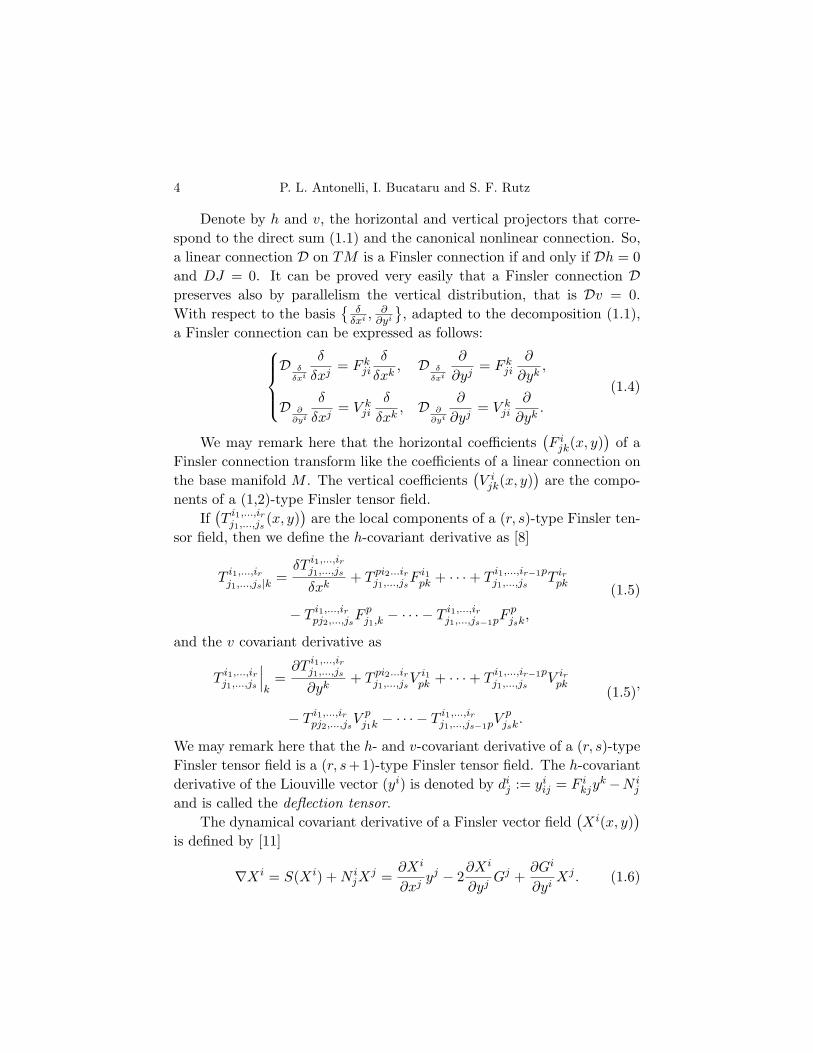
Denote by h and v, the horizontal and vertical projectors that corre-spond to the direct sum (1.1) and the canonical nonlinear connection. So,a linear connection D on TM is a Finsler connection if and only if Dh = 0and DJ = 0. It can be proved very easily that a Finsler connection Dpreserves also by parallelism the vertical distribution, that is Dv = 0.With respect to the basis

δ

δxi ,∂

∂yi

, adapted to the decomposition (1.1),

a Finsler connection can be expressed as follows:

D δ

δxi

δ

δxj= F k

ji

δ

δxk, D δ

δxi

∂

∂yj= F k

ji

∂

∂yk,

D ∂

∂yi

δ

δxj= V k

ji

δ

δxk, D ∂

∂yi

∂

∂yj= V k

ji

∂

∂yk.

(1.4)

We may remark here that the horizontal coefficients(F i

jk(x, y))

of aFinsler connection transform like the coefficients of a linear connection onthe base manifold M . The vertical coefficients

(V i

jk(x, y))

are the compo-nents of a (1,2)-type Finsler tensor field.

If(T i1,...,ir

j1,...,js(x, y)

)are the local components of a (r, s)-type Finsler ten-

sor field, then we define the h-covariant derivative as [8]

T i1,...,irj1,...,js|k =

δT i1,...,irj1,...,js

δxk+ T pi2...ir

j1,...,jsF i1

pk + · · ·+ Ti1,...,ir−1pj1,...,js

T irpk

− T i1,...,irpj2,...,js

F pj1,k − · · · − T i1,...,ir

j1,...,js−1pFpjsk,

(1.5)

and the v covariant derivative as

T i1,...,irj1,...,js

∣∣∣k

=∂T i1,...,ir

j1,...,js

∂yk+ T pi2...ir

j1,...,jsV i1

pk + · · ·+ Ti1,...,ir−1pj1,...,js

V irpk

− T i1,...,irpj2,...,js

V pj1k − · · · − T i1,...,ir

j1,...,js−1pVpjsk.

(1.5)’

We may remark here that the h- and v-covariant derivative of a (r, s)-typeFinsler tensor field is a (r, s+1)-type Finsler tensor field. The h-covariantderivative of the Liouville vector (yi) is denoted by di

j := yiij = F i

kjyk−N i

j

and is called the deflection tensor.The dynamical covariant derivative of a Finsler vector field

(Xi(x, y)

)is defined by [11]

∇Xi = S(Xi) + N ijX

j =∂Xi

∂xjyj − 2

∂Xi

∂yjGj +

∂Gi

∂yiXj . (1.6)


If the deflection tensor of a Finsler connection is zero, then the dy-namical covariant derivative can be expressed as follows:

∇Xi = S(Xi) + F ikjy

kXj = Xi|ky

k. (1.6)’

With respect to the basis(

δδxi ,

∂∂yi

)a Finsler connection has five com-

ponents of torsion ([3], [11]), T kij = F k

ji − F kij , Rk

ij = δN ii

δxj − δNkj

δxi , Ckji,

P kji =

∂N ij

∂yi − F kji, and Sk

ij = V kji − V k

ij . It should be noted that Rkij is called

also the curvature of the nonlinear connection because it is the obstructionfrom being integrable for the nonlinear connection

[δ

δxi ,δ

δxj

]= −Rk

ij∂

∂yk .The only three components of the curvature of a Finsler connection

are given by [3], [10]

Rijk` =

δF ijk

δx`− δF i

j`

δxk+ Fm

jkF im` − Fm

j` F imk + V i

jmRmk`;

P ijk` =

∂F ijk

∂y`− V i

jk|` + V ijmPm

k` ;

Sijk` =

∂V ijk

y`− ∂V i

j`

yk+ V m

jk V im` − V m

j` V imk.

(1.7)

The most important Finsler connections in Finsler geometry are ([3],[9], [11]) the Cartan connection, the Berwald connection, the Chern–Rundconnection, and the Hashiguchi connection. In this paper we shall dealonly with Cartan and Berwald connections.

The Cartan connection is perfectly determined by the axioms [9]:

1 It is metric: gij|k = 0 and gij |k = 0,

2 It is symmetric: T ijk = 0 and Si

jk = 0;

3 The deflection tensor dij vanishes.

The horizontal coefficients of the Cartan connection are given by [11]

F ijk =

12gi`

(δg`j

δxi+

δg`k

δxj− δgjk

δxj

). (1.8)

The vertical coefficients of the Cartan connection are V ijk = Ci

jk, whereCi

jk is the Cartan tensor.


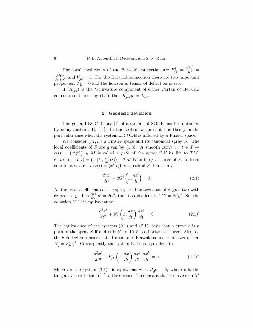
The local coefficients of the Berwald connection are F ijk =

∂N ij

∂yk =∂2Gi

∂yj∂yk and V ijk = 0. For the Berwald connection there are two important

properties: F|i = 0 and the horizontal tensor of deflection is zero.If (Ri

jk`) is the h-curvature component of either Cartan or Berwaldconnection, defined by (1.7), then Ri

jk`yj = Ri

k`.

2. Geodesic deviation

The general KCC-theory [1] of a system of SODE has been studiedby many authors [1], [21]. In this section we present this theory in theparticular case when the system of SODE is induced by a Finsler space.

We consider (M,F ) a Finsler space and its canonical spray S. Thelocal coefficients of S are given by (1.3). A smooth curve c : t ∈ I 7→c(t) =

(xi(t)

) ∈ M is called a path of the spray S if its lift to TM ,c : t ∈ I 7→ c(t) =

(xi(t), dxi

dt (t)) ∈ TM is an integral curve of S. In local

coordinates, a curve c(t) =(xi(t)

)is a path of S if and only if

d2xi

dt2+ 2Gi

(x,

dx

dt

)= 0. (2.1)

As the local coefficients of the spray are homogeneous of degree two withrespect to y, then ∂Gi

∂yj yj = 2Gi, that is equivalent to 2Gi = N ijy

j . So, theequation (2.1) is equivalent to

d2xi

dt2+ N i

j

(x,

dx

dt

)dxj

dt= 0. (2.1)’

The equivalence of the systems (2.1) and (2.1)’ says that a curve c is apath of the spray S if and only if its lift c is a horizontal curve. Also, asthe h-deflection tensor of the Cartan and Berwald connection is zero, thenN i

j = F ijky

k. Consequently the system (2.1)’ is equivalent to

d2xi

dt2+ F i

jk

(x,

dx

dt

)dxj

dt

dxk

dt= 0. (2.1)”

Moreover the system (2.1)” is equivalent with Dec ˙c = 0, where ˙c is thetangent vector to the lift c of the curve c. This means that a curve c on M


is a path of the spray S if and only if c is a geodesic of the Cartan orBerwald connection.

An equivalent invariant form of the system (2.1) is

∇(

dxi

dt

)= 0. (2.2)

Now let c(t) =(xi(t)

)be a path of the spray S and a variation of it into

nearby ones according to

xi(t) = xi(t) + εξi(t). (2.3)

Here ε denotes a scalar parameter with small value |ε|, and ξi(t) are com-ponents of a contravariant vector field along c(t). If we substitute (2.3)into (2.1), ask for c(t) =

(xi(t)

)to be also a path of the spray and let

ε → 0, we get the so-called variational equations

d2ξi

dt2+ 2

∂Gi

∂xjξj + 2

∂Gi

∂yj

dξj

dt= 0. (2.4)

For the variational equation (2.4) we have the equivalent invariant form(Jacobi equation)

∇2ξi + Bijξ

j = 0, where (2.5)

Bij := 2

∂Gi

∂xj− S

(∂Gi

∂yj

)− ∂Gi

∂yk

∂Gk

∂yj= Ri

jkyk. (2.6)

Here (Rijk) is the curvature of the nonlinear connection induced by

canonical spray S. As Rijk = Ri

`jky`, then Bi

j = Ri`jky

`yk. Bij is called the

second invariant of the given SODE, [1] or the Jacobi endomorphism.

Definition 2.1. A Lie symmetry of the spray S is a vector field X onthe base manifold M such that [S,Xc] = 0, where Xc is the complete liftof X and is defined by

if X = Xi(x)∂

∂xi, then Xc = Xi(x)

∂

∂xi+

∂Xi

∂xjyi ∂

∂yj. (2.7)

Theorem 2.1 ([1]). 1. A vector field X = Xi(x) ∂∂xi is a Lie symmetry

of S if and only if

∇2Xi + BijX

j = 0. (2.8)


2. If X = Xi(x) ∂∂xi is a Lie symmetry of S and c(t) =

(xi(t)

)is a

path of S, then the restriction of X along c is a Jacobi vector field.

From (1.6)’ we have that ∇Xi = Xi|jy

j and because yi|j = 0, then the

equation (2.8) is equivalent to

(Xi|j|k + Ri

jmkXm)yjyk = 0. (2.8)’

If we denote by Bij = gikBkj , then Bij = Rìjky

`yk, and consequently Bij

is symmetric with respect to i and j.Let Rìjk the h-curvature component of the Berwald or the Cartan

connection. We define, for a Finsler tensor field Xi(x, y), the flag curva-ture [4]

R(x, y, X) =Rìjky

`ykXiXj

(g`kgij − gìgjk)y`ykXiXj. (2.9)

Denote by ì = 1F yi the normalized supporting element and hij = F ∂2F

∂yi∂yj

the angular metric. It is very easy to prove that the metric tensor and theangular metric are related by gij = hij + ì`j . Then we can rewrite (2.9)as

Bij(x, y)XiXj = R(x, y, X)F 2(x, y)hij(x, y)Xi(x, y)Xj(x, y). (2.10)

Definition 2.2. A Finsler space is said to have scalar curvature R(x, y)if the flag curvature (2.9) does not depend on (Xi) at every point (x, y).From (2.10) we have that a Finsler space has scalar curvature if and onlyif the Jacobi endomorphism can be written as

Bij = RF 2hij . (2.11)

If we denote by hij = gikhkj , then the Jacobi endomorphism of a Finsler

space with scalar curvature can be written as

Bij = RF 2hi

j . (2.11)’

Consequently the Jacobi equation of a Finsler space with scalar curvature,has the form

∇2ξi + RF 2hijξ

j = 0. (2.12)


3. Two dimensional Finsler space

It is well known that every two-dimensional Finsler space has scalarcurvature [9]. Also there is a canonical frame, called the Berwald frame.We shall use this to express the KCC-invariants and study the geodesicdeviation.

Consider (M,F 2) be a two-dimensional Finsler space. Denote by Ci

the length of the Cartan vector Ci and mi = 1C Ci. Then (ì,mi) are uni-

tary vector fields and because ìmi = gij`

imj = 0, then (ì, mi) is an or-thonormal frame, [6]. We call it the Berwald frame of the two-dimensionalFinsler space (M, F 2).

With respect to the Berwald frame, the metric tensor gij and theangular tensor hij are given by

gij = ì`j + mimj , hij = mimj . (3.1)

Proposition 3.1. The local coefficients of the Cartan connection are

given by

F ijk = −`j

δì

δxk−mj

δmi

δxk,

Cijk = −`j

∂ì

yk−mj

∂mi

∂yk+

1F

`jmimk − 1

Fmj`

imk.

(3.2)

Proof. It is known [9] that the h- and v-covariant derivatives of theBerwald frame with respect to the Cartan connection are given by

ì|j = 0; mi

|j = 0;

ì|j =1F

mimj ; mi|j = − 1F

ìmj .(3.3)

¤

If we solve these for F ijk and Ci

jk, then we get (3.2).

Proposition 3.2. The dynamical covariant derivative of the Berwald

frame vanishes identically, that is

∇mi = 0, ∇ì = 0. (3.4)


Proof. According to (1.6)’ the dynamical covariant derivative of ì

is given by ∇ì = ì|jyj , and if we use (3.3) we have (3.4). ¤

Proposition 3.2 says that the Berwald frame is parallel along any pathof the canonical spray.

Let (Xi) be a Finsler vector field, we denote by (X(i)) its scalar com-ponent with respect to the Berwald frame, that is, Xi = X(1)ì + X(2)mi.Then the dynamical covariant derivative of Xi is given by

∇Xi = (X(1))′ì + (X(2))′mi, where (X(1))′ = S(X(1))

and (X(2))′ = S(X(2)).(3.5)

As every two dimensional Finsler space is of scalar curvature we have thatthe Jacobi endomorphism has the form (2.11)’, where R = R1212.

Theorem 3.1. The scalar form of the Jacobi equation (2.5), in a two

dimensional Finsler space with respect to the Berwald frame is given by

(X(1))′′ = 0,

(X(2))′′ + RF 2X(2) = 0.(3.6)

Proof. Let Xi be a Jacobi vector field and denote by (X(i)) its scalarcomponents with respect to the Berwald frame. We have then ∇2Xi =(X(1))′′ì + (X(2))′′mi. Also, as Bi

j = RF 2hij , and hi

j = mimj , then theJacobi equation (2.6) is equivalent to

(X(1))′′ì + (X(2))′′mi + RF 2mimj(X(1)`j + X(2)mj) = 0 ⇐⇒(X(1))′′ì + (X(2))′′mi + RF 2miX(2) = 0 and this is equivalent to (3.6).The equation (3.6) appears also in Rund’s book [13, p. 114], but the wayhe gets it is very complicated.

From (3.6) we can see that the tangential component of every Jacobivector field is of the form (at + b)ì, while the orthogonal component isX(2)mi, where X(2) is the solution of (3.6)2. So if X is a Jacobi vectorfield, then the length squared ‖X(t)‖2 = (at+b)2 +

(X(2)(t)

)2, where X(2)

is the solution of (3.6)2. We can deduce from this that if R > 0 thenthe geodesics are stable (in other words the geodesic rays are bunchingtogether) and if R ≤ 0 then the geodesics are unstable (in other words the


geodesic rays are dispersing). See [4] for more discussion about geodesicstability.

We have to remark here that we can use also (3.6) to find out the Liesymmetries of a two dimensional Finsler space. So a vector field (Xi) is aLie symmetry if and only if its scalar components (X(i)) satisfy (3.6). ¤

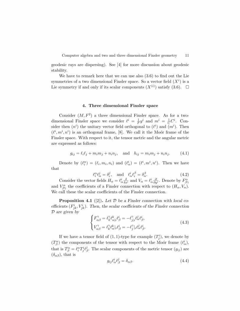
4. Three dimensional Finsler space

Consider (M, F 2) a three dimensional Finsler space. As for a two-dimensional Finsler space we consider ì = 1

F yi and mi = 1C Ci. Con-

sider then (ni) the unitary vector field orthogonal to (ì) and (mi). Then(ì,mi, ni) is an orthogonal frame, [8]. We call it the Moor frame of theFinsler space. With respect to it, the tensor metric and the angular metricare expressed as follows:

gij = ì`j + mimj + ninj , and hij = mimj + ninj . (4.1)

Denote by (`αi ) = (ì,mi, ni) and (ì

α) = (ì,mi, ni). Then we havethat

`αi `j

α = δji , and ì

α`βi = δβ

α. (4.2)Consider the vector fields Hα = ì

αδ

δxi and Vα = ìα

∂∂yi . Denote by Fα

βγ

and V αβγ the coefficients of a Finsler connection with respect to (Hα, Vα).

We call these the scalar coefficients of the Finsler connection.

Proposition 4.1 ([2]). Let D be a Finsler connection with local co-

efficients (F ijk, V

ijk). Then, the scalar coefficients of the Finsler connection

D are given by

F γαβ = `γ

k`kα|i`

iβ = −`γ

j|i`jαì

β,

V γαβ = `γ

k`kα|iì

β = −`γj |i`j

αìβ.

(4.3)

If we have a tensor field of (1, 1)-type for example (T ij ), we denote by

(Tαβ ) the components of the tensor with respect to the Moor frame (ì

α),that is Tα

β = `αi T i

j `jβ. The scalar components of the metric tensor (gij) are

(δαβ), that isgij`

iα`j

β = δαβ . (4.4)


If D is the Cartan connection of the Finsler space, we know that withrespect to it ì

|j = 0, which is the same with ì|j = 0. Then we find from(4.3) that the scalar components Fα

1β vanish.Let us denote by “|α” and “|α” the scalar h-covariant and v-covariant

derivative, respectively. They are given by

Tαβ|γ = Hγ(Tα

β ) + FαδγT δ

β − F δβγTα

δ , and

Tαβ |γ = Vγ(Tα

β ) + V αδγT δ

β −∇δβγTα

δ .(4.5)

The scalar covariant derivative and the covariant derivative are relatedby [2]

Tαβ|γ = T i

j|k`αi `j

β`kγ and Tα

β |γ = T ij |k`α

i `jβ`k

γ . (4.6)

As the fundamental tensor (gij) of a Finsler metric is h- and v-covariantconstant, according to (4.4) and a corresponding formula for (4.5) we havethat

δαβ|γ = gij|kìα`j

β`kγ = 0 and δαβ |γ = gij |kì

α`jβ`k

γ = 0.

From δαβ|γ = 0 we have that δηβF ηαγ+δαηF

ηβγ = 0, so Fα

βγ is skew symmetricwith respect to α and β. As we already have that Fα

1β = 0, then F 1αβ = 0

and Fααβ = 0. The nonzero scalar coefficients of the Cartan connection

are F 32γ = −F 2

3γ . Denote by hj = F 32γ`γ

j . The Finsler vector field hj iscalled the h-connection vector [8]. We denote by T , the scalar FF 3

21, soT = F · F 3

21.

Proposition 4.2. The dynamical covariant derivative of the Moor

frame is given by

∇ì = 0, ∇mi = Tni, and ∇ni = −Tmi. (4.7)

Proof. The h-covariant derivative of the Moor frame with respect toCartan connection is given by [8]

ì|j = 0, mi

|j = nihj , and ni|j = −mihj . (4.8)

As hiyi = F 3

2γ`γi F · ì

1; and `γj `j

1 = δγ1 , we have that hjy

j = FF 321 = T and

(4.7) is true. ¤


Theorem 4.1. A three dimensional Finsler space has scalar curvature

if and only if

Bijmimj = Bijn

inj and Bijminj = 0. (4.9)

Proof. From (2.11) we can see that the Finsler space has scalar cur-vature if and only if Bij = RF 2hij . As Bij is symmetric and Bijy

j = 0,then with respect to Moor frame we have that

Bij = Amimj + B(minj + mjni) + Cninj , where (4.10)

A = Bijmimj , B = Bijm

inj , and C = Bijninj . (4.11)

As hij = mimj + ninj , then a Finsler space has scalar curvature if Bij =RF 2(mimj +ninj). If we compare with (4.10) we have that A = C = RF 2

and B = 0, that is (4.9) is true. ¤

Conversely if (4.9) is true then, Bij = A(mimj + nimj) = Ahij . So,the Finsler space has scalar curvature R = 1

F 2 Bijmimj .

Next we are looking for a scalar version (with respect to Moor frame)of the Jacobi equation (2.5). Consider

(Xi(x, y)

)be a Finsler vector field

with scalar components(X(i)(x, y)

), that is: Xi = X(1)ì + X(2)mi +

X(3)ni. According to Proposition 4.2 we have that the dynamical covariantderivative of (Xi) is given by

∇Xi = (X(1))′ì + [(X(2))′ − T ]mi + [(X(3))′ + T ]ni. (4.12)

Then the second covariant derivative of (Xi) is given by

∇2Xi = (X(1))′′ì + [(X(2))′′ − T ′ − T (X(3))′ − T 2]mi

+ [(X(3))′′ + T ′ + T (X(2))′ − T 2]ni.(4.13)

Theorem 4.2. The scalar form of the Jacobi equation (2.5), in a three

dimensional Finsler space, with respect to Moor frame is given by

(X(1))′′ = 0,

(X(2))′′ − T (X(3))′ + AX(2) + BX(3) − T ′ − T 2 = 0,

(X(3))′′ + T (X(2))′ + BX(2) + CX(3) + T ′ − T 2 = 0.

(4.14)


As for two dimensional Finsler spaces, we can see that the tangentialcomponent of a Jacobi vector field is a solution of (4.14)1, that is (at+b)`i.

If the scalar component F 321 of the Cartan connection vanishes, then

T = 0 and the equations (4.14) become

(X(1))′′ = 0,

(X(2))′′ + AX(2) + BX(3) = 0,

(X(3))′′ + BX(2) + CX(3) = 0.

(4.15)

If the Finsler space has scalar curvature R and F 321 = 0, then we have the

following scalar version of the Jacobi equation (2.5):

(X(1))′′ = 0,

(X(2))′′ + RF 2X(2) = 0,

(X(3))′′ + RF 2X(3) = 0.

(4.16)

In this case we may conclude like in two dimensional case that if the scalarcurvature R is positive, then the geodesics are stable and if R ≤ 0 thenthe geodesics are unstable.

Also we can use the equation (4.14) to determine the Lie symmetriesof a three dimensional Finsler space.

5. Examples(Finsler spaces applied to physics via computer algebra)

Examples of 2 dimensional spaces endowed with a Finsler (non-Rieman-nian) metric, stemming both from applications or pure mathematics, arenot unusual in the literature. We will, therefore, concentrate on providinga higher dimensional example, worked out by means of Computer Algebra,derived from a non-Riemannian version of General Relativity.

A first explicit non-Riemannian solution to a generalized field equation[14] was produced by means of Computer Algebra [15] as the first orderperturbation of the Riemannian 1 parameter family of metrics known as


the Schwarzschild solution (to Einstein’s field equations):

ds2 =dr2

(1− 2m/r)+ r2dΩ2−

(1− 2m

r

)dt2 + ε

(1− 2m

r

)dΩdt, (5.1)

where dΩ =√

dθ2 + sin2 θdφ2 and the perturbation parameter ε is con-sidered small (ε2 ≈ 0). This solution has been obtained by S. F. Rutz in1992 [16].

Both Riemannian (ε = 0) and non-Riemannian (ε 6= 0) families ofmetrics are solutions to vacuum field equations, valid outside matter, andare invariant under SO(3), leading to the so-called spherical symmetry[17], proper to model physical systems such as space-time in the vicinityof massive stars or black holes.

The effect of the parameter m, which stands for the mass of the staror black hole and relates to the curvature of the Riemannian manifold, iswell-known. In order to determine the contribution of the non-Riemannianterm in (5.1), let us take m = 0. In the Riemannian case (ε = 0), thisleads directly to the so-called Minkowski metric, a strictly flat space, withstraight lines as geodesics, a classical model for physical space-time, as de-scribed in Special Relativity. As it is well-known, geodesics represent thetrajectories of test particles or light rays under the action of the gravita-tional field produced by the mass m, is this case, in empty space. But thenotion of straight lines as trajectories of free particles precedes Newton,dating back to Galileo. Nevertheless, just by allowing for non-Riemannianmodels of space-time, one arrives at

ds2 = dr2 + r2dΩ2 − dt2 + εdΩdt, (5.2)

as a possible description for empty space. In what such model differs fromthe classical view? To try to answer this, let us now make use of theComputer Algebra package Finsler [18] to determine the expressions ofsome Finslerian tensors taking (5.2) as input, and considering (ε2 ≈ 0).

5.1. Spray theoretical results. As mentioned before, (5.2) solves a gen-eralized vacuum field equation, this resulting from the fact that Berwald’sdeviation tensor is identically zero up to order ε,

Bij = O(ε2).


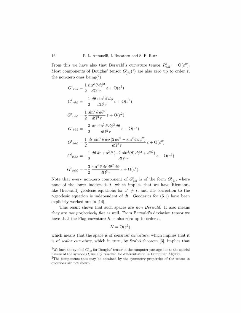
From this we have also that Berwald’s curvature tensor Rijkl = O(ε2).

Most components of Douglas’ tensor Gijkl(

1) are also zero up to order ε,the non-zero ones being(2)

Gtrθθ =

12

sin2 θ dφ2

dΩ3 rε + O(ε2)

Gtrθφ = −1

2dθ sin2 θ dφ

dΩ3 rε + O(ε2)

Gtrφφ =

12

sin2 θ dθ2

dΩ3 rε + O(ε2)

Gtθθθ = −3

2dr sin2 θ dφ2 dθ

dΩ5 rε + O(ε2)

Gtθθφ =

12

dr sin2 θ dφ (2 dθ2 − sin2 θ dφ2)dΩ5 r

ε + O(ε2)

Gtθφφ = −1

2dθ dr sin2 θ (−2 sin2(θ) dφ2 + dθ2)

dΩ5 rε + O(ε2)

Gtφφφ = −3

2sin4 θ dr dθ2 dφ

dΩ5 rε + O(ε2).

Note that every non-zero component of Gijkl is of the form Gt

jkl, wherenone of the lower indexes is t, which implies that we have Riemann-like (Berwald) geodesic equations for xi 6= t, and the correction to thet-geodesic equation is independent of dt. Geodesics for (5.1) have beenexplicitly worked out in [14].

This result shows that such spaces are non Berwald. It also meansthey are not projectively flat as well. From Berwald’s deviation tensor wehave that the Flag curvature K is also zero up to order ε,

K = O(ε2),

which means that the space is of constant curvature, which implies that itis of scalar curvature, which in turn, by Szabo theorem [3], implies that

1We have the symbol Gijkl for Douglas’ tensor in the computer package due to the special

nature of the symbol D, usually reserved for differentiation in Computer Algebra.2The components that may be obtained by the symmetry properties of the tensor inquestions are not shown.


Weyl’s projective tensor is also zero up to order ε, W ijkl = O(ε2). But, as

Douglas’ projective tensor Πijkl = ∂j ∂k∂l(Gi− (1/5)∂aG

axi) is not zero upto order ε, the non-zero components being

Πtrθθ =

12

sin2 θ dφ2

dΩ3 rε + O(ε2)

Πtrθφ = −1

2dθ sin2 θ dφ

dΩ3 rε + O(ε2)

Πtrφφ =

12

sin2 θ dθ2

dΩ3 rε + O(ε2)

Πtθθθ = −3

2dr sin2 θ dφ2 dθ

dΩ5 rε + O(ε2)

Πtθθφ = −1

2dr sin2 θ dφ (−2 dθ2 + sin2 θ dφ2)

dΩ5 rε + O(ε2)

Πtθφφ = −1

2dθ dr sin2 θ (−2 sin2 θ dφ2 + dθ2)

dΩ5 rε + O(ε2)

Πtφφφ = −3

2sin4 θ dr dθ2 dφ

dΩ5 rε + O(ε2),

which implies that these spaces are not projectively Berwald, or not pro-jectively equivalent to a Berwald space.

Finally, the non-zero components of D0jkl = gimxmGi

jkl, are

D0rθθ = −1

2dt sin2 θ dφ2

dΩ3 rε + O(ε2)

D0rθφ =

12

dt dθ sin2 θ dφ

dΩ3 rε + O(ε2)

D0rφφ = −1

2dt sin2 θ dθ2

dΩ3 rε + O(ε2)

D0θθθ =

32

dt dr sin2 θ dφ2 dθ

dΩ5 rε + O(ε2)

D0θθφ =

12

dt dr sin2 θ dφ (−2 dθ2 + sin2 θ dφ2)dΩ5 r

ε + O(ε2)


D0θφφ =

12

dt dθ dr sin2 θ (−2 sin2 θ dφ2 + dθ2)dΩ5 r

ε + O(ε2)

D0φφφ =

32

dt sin4 θ dr dθ2 dφ

dΩ5 rε + O(ε2)

what tells us that such spaces are non Landsberg.So, in a spray-like perspective, we have that the geodesics of (5.2) are

corrected only for the t coordinate, that such correction is independent ofdt, and that the geodesics deviate linearly from one another. In partic-ular this last feature connects our model to the classical intuition abouttrajectories in empty space-time.

We say (5.2) is an almost flat space, since Rijkl = 0 and most compo-

nents of Dijkl are also zero, in the given order of approximation.

5.2. Cartan-type metrical results. In a metrical perspective, usingCartan’s formalism for Finsler spaces, we have, to begin with, that Car-tan’s tensor Cijk is not only nonzero, but actually proportional to theperturbation parameter ε,

Cθθθ = −32

dt sin2 θ dφ2 dθ

dΩ5ε

Cθθφ =12

dt sin2 θ dφ (2 dθ2 − sin2 θ dφ2)dΩ5

ε

Cθθt =12

sin2 θ dφ2

dΩ3ε

Cθφφ = −12

dt dθ sin2 θ (−2 sin2 θ dφ2 + dθ2)dΩ5

ε

Cθφt = −12

dθ sin2 θ dφ

dΩ3ε

Cφφφ = −32

dt sin4 θ dθ2 dφ

dΩ5ε

Cφφt =12

sin2 θ dth2

dΩ3ε.

This tells us that spaces endowed with (5.2) as metric function are notRiemannian. Actually, such spaces would be Riemannian if and only if


ε = 0, when would have a Minkowski metric (in the relativistic sense).The same is true for (5.1), which is Riemannian if and only if ε = 0, whenwe would have the Schwarzschild metric.

The fact that spaces with a metric as (5.2) are non-Landsberg, asstated before, gives us that Cartan’s curvature tensor P i

jkl is not zero upto order ε. But we have that Cartan’s curvature tensor Si

jkl is identicallyzero up to the same order,

Sijkl = O(ε2).

This result implies that the curvature of the tangent spaces to (5.2) is zero,that is, given a fixed point in the manifold one could find yi-coordinatessuch that the tangent space at that point is Euclidean, as in Riemann-ian spaces. Note that such yi-transformations are not allowed in Finslerspaces independently of its correspondent xi-transformations, such beingconsidered as an illustration here.

Note also that Brickell’s theorem [5], that says that Sijkl = 0 impliesthat the space must be Riemannian, does not apply here, since (5.2) isnot positive-definite. The metric (5.2) thus provide an example of howBrickell’s theorem fails if its assumptions, particularly regarding positive-definiteness, are not met.

As for the third Cartan’s curvature tensor, Rijkl, given as RCi

jkl in theoutput below to differ from Berwald’s curvature tensor Ri

jkl, is not zeroup to order ε. For instance, the component

RC rθrθ =

12

dt sin2 θ dφ2

dΩ3 r2ε + O(ε2).

This shows that, although (5.2) is a first order departure of a Riemannianflat space, we have that only 1 among the 3 Cartan’s curvature tensors,namely Sijkl, is zero in the same order of approximation.

The full description of the metrical properties of (5.2) will be givenelsewhere [20].

5.3. Frame fields. In order to express (5.2) in terms of frame fields, ortetrads, as such fields are known in Relativity, let us now first look at the 3dimensional metric produced by taking the coordinate r to be constant,or dr = 0, thereby still preserving the non-Riemannian character in

ds23 = r2dΩ2 − dt2 + εdΩdt. (5.3)


The Moor frame for such 3 dimensional metric is given, up to firstorder of approximation in ε, by

n1 θ =dθ

(r2dΩ2 − dt2)(1/2)− 1

2dθ dΩ dt

(r2dΩ2 − dt2)(3/2)ε + O(ε2)

n1φ =dφ

(r2dΩ2 − dt2)(1/2)− 1

2dφ dΩ dt

(r2dΩ2 − dt2)(3/2)ε + O(ε2)

n1 t =dt

(r2dΩ2 − dt2)(1/2)− 1

2dt2 dΩ

(r2dΩ2 − dt2)(3/2)ε + O(ε2)

n2 θ =− dθ dt dΩr√−r2dΩ2 + dt2 (−dΩ2)

− 12

dθ r (−dΩ2)(−r2dΩ2 + dt2)(3/2)

ε + O(ε2)

n2φ =− dφ dt dΩr√−r2dΩ2 + dt2 (−dΩ2)

− 12

dφ r (−dΩ2)(−r2dΩ2 + dt2)(3/2)

ε + O(ε2)

n2 t =− dΩr

r√−r2dΩ2 + dt2 (−dΩ2)

+12

dt3

(−r2dΩ2 + dt2)(3/2)ε + O(ε2)

n3 θ =− dθ dtr dΩ

√−r2dΩ2 + dt2+

12

√−r2dΩ2 + dt2 (−dΩ) dθ r

(r2dΩ2 − dt2)2ε + O(ε2)

n3φ =− dφ dtr dΩ

√−r2dΩ2 + dt2+

12

√−r2dΩ2 + dt2 (−dΩ) dφ r

(r2dΩ2 − dt2)2ε + O(ε2)

n3 t =− −dΩ2 r

dΩ√−r2dΩ2 + dt2

− 12

√−r2dΩ2 + dt2 − dt3

r(r2dΩ2 − dt2)2ε + O(ε2).

The frame above reproduce the metric (5.3) in the given order of approx-imation, as

ds23 = (n1in1i + n2in2j + n3in3j)dxidxj ,

with dxi = dθ, dφ, dt. In order to produce the actual frame for the 4dimensional metric (5.2), we may use the Collaring theorem from Differ-ential Topology to claim that there exists a vector field in the 4 dimensionalFinsler space given by (5.2) which is normal to its subspace dr = 0, givenby (5.3). It is important to note that the fact that a Finsler metric like(5.2) can be expressed in terms of a frame field, thus pointing out to the


generalization of the powerful calculus in tetrad fields from its usual Rie-mannian framework in General Relativity to Finsler spaces, is of centralimportance to the development of generalized theories of gravity, that mayallow for non straight behavior of particle trajectories in empty space-time,such as has been recently suggested by deep space observations.

As further steps, we want to determine such a frame field, and alsoto similarly work out the (tetrad) frame field for the 4 dimensional met-ric (5.1), and therefore proceed to determine an axially symmetric non-Riemannian solution to the generalized gravitational field equation, in theline described in [19].

Acknowledgement. The second author would like to thankDr. P. L. Antonelli for his support as a Postdoc at the Universityof Alberta. The third author acknowledges the support of the Braziliangovernment research support agency CNPq. The authors would like tothank Mrs. Vivian Spak for her excellent typesetting.

Appendix

A1. If F is the fundamental function of a Finsler space then.

(1) gij := 12

∂2F 2

∂yi∂yj is the metric tensor, (gij) the inverse;

(2) Gi := 14 gij

(∂2F 2

∂yj∂xm ym − ∂F 2

∂xj

)are the local coefficients of the canonical

spray;

(3) N ij := ∂Gi

∂yj are the local coefficients of the canonical nonlinear connec-tion;

(4) δδxi := ∂

∂xi −N ji

∂∂yh is the h-operator of differentiation;

(5) Rijk =

δN ij

δxk − δN ik

δxj is the curvature of the nonlinear connection (if Rijk = 0

the nonlinear connection is integrable);

(6) Bij := Ri

jkyk is the second invariant in KCC-theory;

Bij := gikBkj (should be symmetric, its first eigenvalue is always zero);

(7) hij = F ∂2F∂yi∂yj is the angular metric (determinant of hij is 0) (if Bij

and hij are proportional, then the Finsler space has scalar curvatureR = 1

F 2

Bij

hij);


(8) Cijk = 12

∂gij

∂yk and Cijk = gi`C`jk are Cartan tensors;

(9) Ci = Cijkg

jk is the Cartan vector;

(10) C = (CiCjgij)1/2 is the length of the Cartan vector;

(11) ì = 1F yi is the normalized supporting element; (we have that gij =

hij + ì`j)

A2. Two dimensional Finsler space.

(12) mi = 1C Ci; ì and mi are orthogonal, that is, gij`

imj = 0 (ì,mi) iscalled the Berwald frame;

(13) F ijk = −`j

δì

δxk −mjδmi

xk are the horizontal coefficients of the Cartanconnections (are symmetric): F i

jk = F ikj and ì = gij`

j and mi =gijm

j ;

(14) Cijk = −`j

∂ì

∂yk −mj∂mi

∂yk + 1F `jm

imk − 1F mj`

imk are the verticalcomponents of the Cartan connection.

(15) Here we have that Bij = RF 2hij = RF 2mimj (check), evaluate R. Ifa vector field (Xi) has the components X(1) and X(2) with respect to

Berwald frame then

(X(1))′ = 0,

(X(2))′′ + RF 2X(2) = 0.

A.3. Three dimensional Finsler spaces.

ì and mi are from (11) and (12).

(16) g = det (gij)

(17)

n1 = g−1/2(`2m3 − `3m2)

n2 = g−1/2(`3m1 − `1m3)

n3 = g−1/2(`1m2 − `2m1)(ni) is a unitary vector field: gijn

inj = 1 (ì,mi, ni) is an orthogonalbase, called the Moor base.

(18)

A = Bijmimj

B = Bijminj

C = Bjijninj

if A = C and B = 0 the space has scalar curvature R = 1F 2 A.


(19) T :=(

∂m1

∂xj yj − 2 ∂m1

∂yj Gj)/n1 ( 1

F T = F 321 a scalar component of the

Cartan connection).

(20) If T = 0 then the scalar components (X(i)), with respect to Moorframe, of a Jacobi vector field are solutions of

(X(1))′′ = 0,

(X(2))′′ + AX(2) + BX(3) = 0,

(X(3))′′ + BX(2) + CX(3) = 0.

(21) If T 6= 0 the scalar components of a Jacobi vector field are given by

the system

(X(1))′′ = 0,

(X(2))′′ − T (X(3))′ + AX(2) + BX(3) − T ′ − T 2 = 0,

(X(3))′′ + T (X(2))′ + BX(2) + CX(3) + T ′ − T 2 = 0.

References

[1] P. L. Antonelli and I. Bucataru, New results about the geometric invariantsin KCC-theory, Handbook on Finsler Geometry, (P. L. Antonelli, ed.), KluwerAcademic Press (to appear).

[2] P. L. Antonelli and I. Bucataru, On Holland’s frame for Randers space andits applications in Physics, Steps in Differential Geometry, (Kozma, L., Nagy, P.T.,and Tamassy, L., eds.), Proceedings, Debrecen, 2000.

[3] P. L. Antonelli R. S. Ingarden and M. Matsumoto, The Theory of Spraysand Finsler Spaces with Applications in Physics and Biology, Kluwer AcademicPress, Dordrecht, 1993, 350.

[4] D. Bao, S. Chern and Z. Shen (eds.), Finsler geometry, Seattle Conference, 1995,Vol. 196, Contemporary Mathematics, Series of Amer. Math. Soc., Providence,R.I., 1995.

[5] D. Bao, S. Chern and Z. Shen, An Introduction to Riemann-Finsler Geometry,Springer-Verlag, Berlin, 2000.

[6] L. Berwald, On Finsler and Cartan geometries III, Two-dimensional Finsler spaceswith rectilinear extremals, Ann. of Math. 42 (1941), 84–112.

[7] F. Grifone, Structure prescue-tangente et connexions I, II, Ann. Inst. HenriPoincare 22, 1 (1972), 287–334; 22, 3 (1972), 291–338.

[8] M. Matsumoto, A theory of three-dimensional Finsler spaces in terms of scalars,Demonstratio Matematica VI (1972), 223–225.

[9] M. Matsumoto, Foundations of Finsler Geometry and Special Finsler Spaces,Kaiseisho Press, Japan, 1986.

[10] A. Moor, Quelques remorques sur le generalisation du scalare de courlure et duscalaire principal, Canad. J. Math. 4 (1952), 189–197.

[11] R. Miron and M. Anastasiei, The Geometry of Lagrange Spaces: Theory andApplications, Kluwer Academic Press, Dordrecht, 1994.

24 P. L. Antonelli et. al : Computer algebra and two and three. . .

[12] R. Miron and H. Izumi, Invariant frame in generalized metric spaces, Tensor, N.S.42 (1985), 272–282.

[13] H. Rund, The Differential Geometry of Finsler Spaces, Springer Verlag, Berlin,1959.

[14] S. F. Rutz, A Finsler Generalisation of Einstein’s Vacuum Field Equations, Gen.Rel. Grav. 25 (1993), 1139–1158.

[15] S. F. Rutz, Symmetry and Gravity in Finsler Spaces, thesis, Queen Mary & West-field College, University of London, 1993.

[16] S. F. Rutz, A Finsler Generalisation of Einstein’s Vacuum Field Equations, Rela-tivity Seminars, School of Mathematical Sciences, Queen Mary & Westfield College,University of London, 1992.

[17] S. F. Rutz and P. J. McCarthy, The General Four Dimensional SphericallySymmetric Finsler Metric, Gen. Rel. Grav. 25 (1993), 589–602.

[18] S. F. Rutz and R. Portugal, Finsler: A Computer Algebra Package for FinslerGeometries, Nonlinear Analysis 47 (2001), 6121–6134.

[19] S. F. Rutz and F. M. Paiva, Gravity in Finsler Spaces, Finslerian Geometries: AMeeting of Minds, Kluwer, Dordrecht, 2000, 233–244.

[20] S. F. Rutz and R. Portugal, Finsler: A Computer Algebra Package for FinslerGeometries, Handbook on Finsler Geometry, (Antonelli, P. L., ed.), Kluwer Aca-demic Press (to appear).

[21] Z. Shen, Geometric methods for second order ordinary differential equations,Preprint.

P. L. ANTONELLI

DEPARTMENT OF MATHEMATICAL SCIENCES

UNIVERSITY OF ALBERTA

EDMONTON, ALBERTA

CANADA T6G 2G1

E-mail: [email protected]

I. BUCATARU

FACULTY OF MATHEMATICS

“AL.I.CUZA” UNIVERSITY

IASI 6600

ROMANIA


S. F. RUTZ

COPPE-SISTEMAS, UFRJ

CXP 68511, RIO DE JANEIRO, RJ 21945-970

BRAZIL


(Received October 22, 2002; revised February 3, 2003)

computer algebra and two and three dimensional finsler...

Documents