James Freeman, Klaus Hellgardt, Christos N. Markides

AN ASSESSMENT OF A SOLAR-POWERED

ORGANIC RANKINE CYCLE SYSTEM FOR

COMBINED HEATING AND POWER IN

DOMESTIC APPLICATIONS

SusTEM Special Sessions

on

Thermal Energy Management

Department of Chemical Engineering,

Imperial College London, UK

Background

Organic Rankine Cycle (ORC) is a

proven technology for the generation

of power from low grade solar and

waste heat sources.

Challenges exist to develop this

technology for the small (domestic)

scale, and as part of an integrated

system for the provision of combined

heat and power.

Further specific challenges are

presented by the nature of the UK

climate and solar resource.

• To develop a techno-economic model of a domestic (small-scale)

combined solar heating and power (CSHP) system featuring an organic

Rankine cycle (ORC) with a generalised positive displacement

expander.

• To model the performance of the system in the UK climate over an

annual period.

• To evaluate the levelised cost of electricity produced over the system

lifetime, the additional thermal energy produced, and the potential for

CO2 emissions reduction.

Objectives

Overview of system model

Overview of system model

1 2

3 4

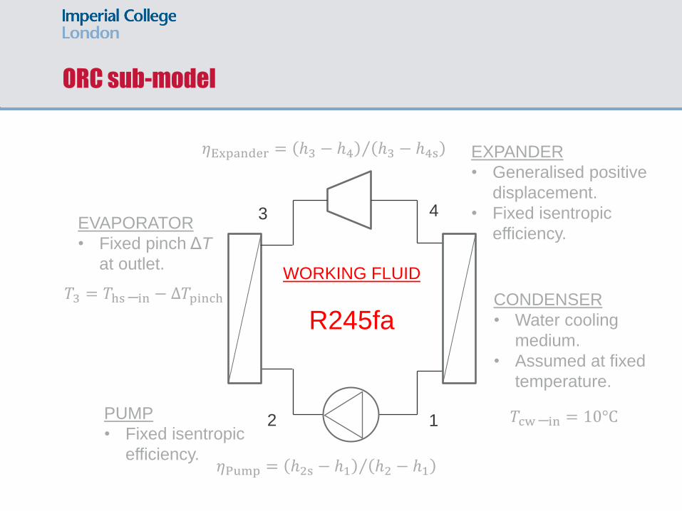
ORC sub-model

1 2

3 4

PUMP

• Fixed isentropic

efficiency. 𝜂Pump = ℎ2s − ℎ1 ℎ2 − ℎ1

ORC sub-model

EVAPORATOR

• Fixed pinch ΔT

at outlet.

1 2

3 4

PUMP

• Fixed isentropic

efficiency. 𝜂Pump = ℎ2s − ℎ1 ℎ2 − ℎ1

𝑇3 = 𝑇hs−in − ∆𝑇pinch

ORC sub-model

EXPANDER

• Generalised positive

displacement.

• Fixed isentropic

efficiency. EVAPORATOR

• Fixed pinch ΔT

at outlet.

1 2

3 4

PUMP

• Fixed isentropic

efficiency. 𝜂Pump = ℎ2s − ℎ1 ℎ2 − ℎ1

𝑇3 = 𝑇hs−in − ∆𝑇pinch

𝜂Expander = ℎ3 − ℎ4 ℎ3 − ℎ4s

ORC sub-model

EXPANDER

• Generalised positive

displacement.

• Fixed isentropic

efficiency. EVAPORATOR

• Fixed pinch ΔT

at outlet.

CONDENSER

• Water cooling

medium.

• Assumed at fixed

temperature.

1 2

3 4

PUMP

• Fixed isentropic

efficiency. 𝜂Pump = ℎ2s − ℎ1 ℎ2 − ℎ1

𝑇3 = 𝑇hs−in − ∆𝑇pinch

𝜂Expander = ℎ3 − ℎ4 ℎ3 − ℎ4s

𝑇cw−in = 10°C

ORC sub-model

EXPANDER

• Generalised positive

displacement.

• Fixed isentropic

efficiency. EVAPORATOR

• Fixed pinch ΔT

at outlet.

CONDENSER

• Water cooling

medium.

• Assumed at fixed

temperature.

1 2

3 4

PUMP

• Fixed isentropic

efficiency.

WORKING FLUID

R245fa

𝜂Pump = ℎ2s − ℎ1 ℎ2 − ℎ1

𝑇3 = 𝑇hs−in − ∆𝑇pinch

𝜂Expander = ℎ3 − ℎ4 ℎ3 − ℎ4s

𝑇cw−in = 10°C

ORC sub-model

𝜂collector = 𝑐0 − 𝑐1 ∙𝑇 𝑐𝑜𝑙𝑙𝑒𝑐𝑡𝑜𝑟 − 𝑇ambient

𝐼𝑠𝑜𝑙ar− 𝑐2 ∙

𝑇 collector − 𝑇𝑎𝑚𝑏𝑖𝑒𝑛𝑡2

𝐼𝑠𝑜𝑙ar

𝑇ambient

𝑇outlet 𝑇inlet

𝐼solar

𝜂𝑐𝑜𝑙𝑙𝑒𝑐𝑡𝑜𝑟 ∙ 𝐼𝑠𝑜𝑙𝑎𝑟 ∙ 𝐴collector = 𝑚 fluid ∙ 𝑐𝑝∙ 𝑇outlet − 𝑇in𝑙𝑒𝑡

𝑚 fluid

𝑇 collector = 𝑇outlet + 𝑇inlet /2

𝐴collector = 15 m2 (DECC)

Solar collector sub-model

Assume quasi-equilibrium:

Non-concentrating collector

• Evacuated tube technology.

• Non-tracking.

• Model using global irradiance data on a tilted

plane.

Concentrating collector

• Parabolic trough technology.

• Tracking and non-tracking case.

• For tracking case use direct-beam irradiance data on

a perfect-tracking plane.

• For non-tracking case use direct-beam on a fixed

plane.

Solar collector data

𝑀tank𝑐p,wd𝑇tankd𝑡

= 𝑞 solar − 𝑞 loss − 𝑞 demand

Capacity = 150 litres.

Dimensions: 1.5 m (height) x 0.36m (ø).

𝑞 solar = 𝑚 coil 𝑐p,w 𝑇coil−in − 𝑇coil−out .

𝑚 coil, 𝑇coil−in

𝑚 coil, 𝑇coil−out

𝑞 demand = 𝑚 coil 𝑐p,w 𝑇supply − 𝑇mains−inlet

𝑞 loss

𝑇room = 20 °C

U-value = 3 W/(m2K).

𝑇coil−out = 𝑇hwc + ∆𝑇pinch .

∆𝑇pinch = 5 °C

𝑞 loss

𝑇tank

Thermal store sub-model

SOLAR THERMAL

COLLECTOR

WATER HEATING

CIRCUIT

ORGANIC

RANKINE CYCLE

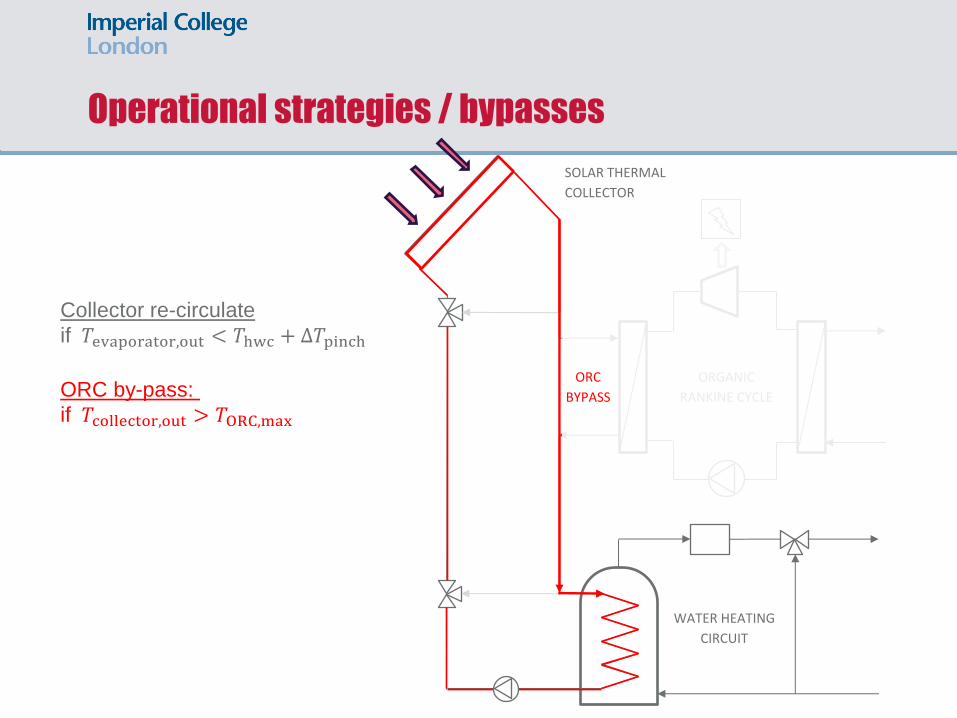
Operational strategies / bypasses

SOLAR THERMAL

COLLECTOR

COLLLECTOR

RECIRCULATE

WATER HEATING

CIRCUIT

ORGANIC

RANKINE CYCLE

Collector re-circulate

if 𝑇evaporator,out < 𝑇hwc + ∆𝑇pinch

Operational strategies / bypasses

SOLAR THERMAL

COLLECTOR

WATER HEATING

CIRCUIT

ORGANIC

RANKINE CYCLE

ORC

BYPASS

Collector re-circulate

if 𝑇evaporator,out < 𝑇hwc + ∆𝑇pinch

ORC by-pass:

if 𝑇collector,out > 𝑇ORC,max

Operational strategies / bypasses

SOLAR THERMAL

COLLECTOR

TANK BYPASS

WATER HEATING

CIRCUIT

ORGANIC

RANKINE CYCLE

Collector re-circulate

if 𝑇evaporator,out < 𝑇hwc + ∆𝑇pinch

ORC by-pass:

if 𝑇collector,out > 𝑇ORC,max

Tank by-pass:

if 𝐹𝑐𝑜𝑖𝑙 < 1

Operational strategies / bypasses

SOLAR THERMAL

COLLECTOR

WATER HEATING

CIRCUIT

ORGANIC

RANKINE CYCLE

Collector re-circulate

if 𝑇evaporator,out < 𝑇hwc + ∆𝑇pinch

ORC by-pass:

if 𝑇collector,out > 𝑇ORC,max

Tank by-pass:

if 𝐹𝑐𝑜𝑖𝑙 < 1

Rejected heat recovery:

if 𝑚 ℎ𝑤,𝑑𝑒𝑚𝑎𝑛𝑑 > 0

RECLAIM

REJECTED HEAT

Operational strategies / bypasses

SOLAR THERMAL

COLLECTOR

WATER HEATING

CIRCUIT

ORGANIC

RANKINE CYCLE

Collector re-circulate

if 𝑇evaporator,out < 𝑇hwc + ∆𝑇pinch

ORC by-pass:

if 𝑇collector,out > 𝑇ORC,max

Tank by-pass:

if 𝐹𝑐𝑜𝑖𝑙 < 1

Rejected heat recovery:

if 𝑚 ℎ𝑤,𝑑𝑒𝑚𝑎𝑛𝑑 > 0

RECLAIM

REJECTED HEAT

Operational strategies / bypasses

• Cycle evaporation pressure (2 – 30 bar)

• Cycle condensation temperature (15 – 25 °C)

• Working fluid mass flow-rate (0.005 – 0.03 kg/s)

• Collector fluid mass flow-rate (0.005 – 0.07 kg/s)

• % bypass of hot-water cylinder (0 – 100%)

• Type of collector (concentrating/non-concentrating)

• Climate data Irradiance, air temperature

• Demand data Electricity, hot water

Model input variables

• Use model to size components based on required flow rates,

pressures, available roof area etc.

• Market survey to obtain costs for:

solar array

ORC components

domestic hot water cyclinder

ancillary plumbing/installation items

• Calculate the installed cost per unit generating capacity

(£/We) and the Levelised Cost of Electricity (LCoE, £/kWhe).

• Calculate additional hot water production available.

Cost analysis

Rotary screw

compressor

Rotating vane air

compressor

HVAC scroll

compressor

Reciprocating

air compressor

Expander/compressor study

Maximum exergy production from solar collector

.

𝑊 max = 𝐻 sc−out − 𝐻 0 −𝑇0 𝑆 sc−out − 𝑆 0

− d𝑊 = 𝜂Carnot 𝑚 𝑐 ∙ d𝑇sc−out 𝑇0

𝑇sc−out

∆𝐻 = ∆𝑄 sc = 𝜂sc𝐼sol𝐴sc

0 100 200 300 4000

100

200

300

400

Collector outlet temperature [C]

wm

ax [

W]

Parabolic trough

Evacuated tube

Isol = 120 W/m2

Asc = 15m2

Exergy analysis: Reversible vs. endo-reversible

Qh

Qc

W

Th

Tc

Qh

Qc

Th,c

Tc,c

Th,r

Tc,r

W

Maximum power for a 15 m2 solar collector array evaluated over an annual period:

𝑊 max = 192 W when evaluated for reversible Carnot engine

(this is the ideal maximum for this collector).

𝑊 max = 106 W when evaluated for endo-reversible Curzon-Ahlborn engine

(this is a practical expectation for this collector).

Difference in annual exergy production between parabolic trough and evacuated

tube is very small!

Parametric analysis

• Comparison between collector types:

PTC fixed = parabolic tough (concentrating) collector, fixed-orientation.

PTC tracking = parabolic trough collector with ideal 2-axis tracking.

ETC fixed = evacuated tube (non-concentrating) collector, fixed orientation.

• Mass flow rates and operating pressures set for maximum power output from

system for a given collector.

• Maximum power settings for the system affected by the choice of collector

e.g. parabolic trough collector operates at higher temperature hence higher ORC

evaporation pressure.

Parametric analysis – ORC evaporation pressure

0 5 10 15 20 25 300

20

40

60

80

ORC evaporation pressure [bar]

PO

RC [

W(e

)] (

ave

rag

e)

PTC. tracking. msc

= 0.02 kg/s. mwf

= 0.01 kg/s

PTC. fixed. msc

= 0.02 kg/s. mwf

= 0.01 kg/s

ETC. fixed. msc

= 0.03kg/s. mwf

= 0.01 kg/s

Parametric analysis – Solar fluid mass flow rate

0 0.01 0.02 0.03 0.04 0.05 0.060

20

40

60

80

Solar collector fluid mass flow rate [kg/s]

PO

RC [

W(e

)] (a

vera

ge)

PTC, tracking. p2= 18 bar. m

wf= 0.01 kg/s

PTC. fixed. p2= 18 bar. m

wf= 0.01 kg/s

ETC. fixed. p2= 10 bar. m

wf= 0.01 kg/s

Parametric analysis – ORC fluid mass flow rate

0.005 0.01 0.015 0.02 0.025 0.030

20

40

60

80

ORC working fluid mass flow rate [kg/s]

PO

RC [

W(e

)] (a

vera

ge)

PTC, tracking. P2= 18 bar. m

sc= 0.02 kg/s

PTC. fixed. P2= 18 bar. m

sc= 0.02 kg/s

ETC. fixed. P2= 10 bar. m

sc= 0.03 kg/s

Parametric analysis – ORC condensation temperature

15 20 25 30 350

20

40

60

80

ORC condensation temperature [C]

PO

RC [

W(e

)] (a

vera

ge)

PTC, tracking. P2= 18 bar. m

sc= 0.02 kg/s. m

wf= 0.01 kg/s.

PTC. fixed. P2= 18 bar. m

sc= 0.02 kg/s. m

wf= 0.01 kg/s.

ETC. fixed. P2= 10 bar. m

sc= 0.03 kg/s. m

wf= 0.01 kg/s.

Parametric analysis – Hot water provision

0 20 40 60 80 1000

20

40

60

80

Collector fluid flow to hot water cylinder heating coil [%]

PO

RC [

W(e

)] (a

vera

ge)

PTC. tracking.

PTC. fixed.

ETC. fixed.

Performance analysis - 24 hour period

4 6 8 10 12 14 16 18 200

100

200

300

400

500

600

Time [hour]

PO

RC [

W(e

)]

PTC. tracking. P2= 18 bar. m

sc= 0.02 kg/s. m

wf= 0.01 kg/s

ETC. fixed. P2= 10 bar. m

sc= 0.03 kg/s. m

wf= 0.01 kg/s

Intermittent operation observed for a fixed flow rate system:

Results of annual simulation with fixed flow rates

PTC tracking

PTC fixed

ETC fixed

Average electrical output We (avg) 75 44 67

Installed cost per We £/We (avg) 61.5 103.8 37.1

Peak electrical output We (peak) 386 384 321

Total annual electrical output kWeh/yr 657 389 588

% annual electrical demand % 19.9 11.8 17.8

ORC switch-on temperature °C 137 137 105

ORC operation time hr/yr 1836 1090 2080

Cooling water consumption m3/yr 834 502 956

Avg solar collector efficiency* % 46.5 31.3 51.5

Avg ORC efficiency % 14.2 14.2 11.9

Initial investment cost £ 4614 4615 2489

Annual incurred (O&M) cost £/yr 46 46 25

Levelised cost of electricity £/kWh 0.80 1.36 0.49

Payback time years 13.9 14.8 9.3

Annual CO2 emission savings kgCO2/yr 391 251 355

*Reported value is the mean solar collector efficiency during ORC operational hours only, and

normalised relative to the global (diffuse + direct) solar irradiance on a horizontal surface.

Summary and conclusions

• Assessment of a small-scale combined solar heat and power system based on

organic Rankine cycle technology for domestic use in the UK.

• System model based on simple component efficiency data, load profiles and

operational control regimes.

• Annual simulation results for a fixed flow-rate system with a 15 m2 solar collector

array show an average power output in the region 65-75 We(avg).

• Installed cost of system in the region £2500-4500.

• Cost per unit power 37-62 £/We(avg) compared to 20-30 £/We(avg) for solar-PV.

• Potential to achieve a further ~30% increase in power output from the system

through optimisation of ORC design and control of system flow rates.

Planned future developments

• Control of system including variable flow rates

• Options for heat rejection

• Consideration of most appropriate working fluid or mixture

• Consideration of appropriate expanders for small-scale ORC

• Further consideration of solar collector design

• Experimental validation of solar collector and ORC sub-models

• Combined levelised-cost comparison with PV and Hybrid PV-T

Next step: variable flow rate control

• Prevent periodic on-off switching of system by not extracting too

much heat from the collector fluid.

• Modify 𝑚 wf so that 𝑄 ORC−in ≤ 𝑄 collector−in.

• 8% increase in annual work production achieved.

6 8 10 12 14 16 180

50

100

150

200

250

300

350

Time [hour]

Pe

l [W

]

Fixed WF flow rate, 0.01 kg/s

Variable WF flow rate

4 6 8 10 12 14 16 18 200

20

40

60

80

100

120

140

160

Time [hour]T

sc-o

ut [ C

]

Fixed WF flow rate, 0.01 kg/s

Variable WF flow rate

Thank you.

S. Canada, G. Cohen, R. Cable, D. Brosseau, and H. Price, “Parabolic trough organic Rankine cycle solar

power plant”, in DOE Solar Energy Technologies Program Review Meeting, (Denver, USA), 2004.

Department for Energy and Climate Change (DECC). 2012. Personal communication with authors.

P. Owen, “Powering the Nation. Household electricity-using habits revealed.” Energy Saving Trust, 2012.

S. Quoilin, M. Orosz, H. Hemond, and V. Lemort, “Performance and design optimization of a low-cost solar

organic Rankine cycle for remote power generation”, Solar Energy, vol. 85, no. 5, pp. 955-966, 2011.

Office of Gas and Electricity Markets, “Typical domestic energy consumption gures factsheet." [Online], 2011.

Available: http://www.ofgem.gov.uk

Solartechnik Prϋfung Forschung, “Collector catalogue." CD, 2002. Produced by Institut fr Solartechnik SPF,

Rapperswil, Berne.

M. Suri, T. A. Huld, E. D. Dunlop, and H. A. Ossenbrink, “Potential of solar electricity generation in the

European Union member states and candidate countries”, Solar Energy, vol. 81, no. 10, pp. 1295-1305, 2007.

W. Weiss and M. Rommel, “Process heat collectors. State of the art within task 33/IV”, IEA Solar Heating and

Cooling Programme, 2008.