am ii basic macroeconomic model - wifa.uni-leipzig.de · institut für theoretische...

Institut für Theoretische VolkswirtschaftslehreMakroökonomik

Prof. Dr. Thomas StegerAdvanced Macroeconomics II | Lecture| SS 2013

1 Basic Macroeconomic Models

Textbook (static) macromodel

1. Basic Macroeconomic Models

Textbook (static) macromodel

Dynamic AS-AD model

Basic dynamic macromodel with expectations

Schools of macroeconomic thoughtg


Basic Macroeconomic Models

P li i i (1)Preliminaries (1)

Macroeconomics: two defining characteristicsMacroeconomics: two defining characteristics studies the economic interactions in society as a whole

aims at understanding empirical regularities in the behavior of aggregate aims at understanding empirical regularities in the behavior of aggregate economic variables such as production, investment, unemployment, price level…

Macroeconomics: three purposes explain the level of the aggregate variables as well as their movement over

time in the short run and the long run

make well founded forecasts possible make well-founded forecasts possible

provide foundations for rational macroeconomic policy

2



P li i i (2)Preliminaries (2)

The short run… concentrates on the behavior of the macroeconomic variables within a time horizon of a few years. focuses on mechanisms that determine how fully an economy uses its productive capacity and are

typically demand dominated. shifts in aggregate demand tend to be accommodated by changes in the produced quantities

rather than in the prices of goods.

Th l The long run… deals with a time horizon long enough such that changes in the capital stock, population, and

technology have a dominating influence on the level of production. uses analytical frameworks which are supply dominated. Variations in the employment rate for

labor and capital due to demand fluctuations are ignored.

The medium run The medium run… medium run models (business cycle models) attempt to understand the pattern of economic

fluctuations. focuses on the dynamic interaction between demand and supply factors

3

focuses on the dynamic interaction between demand and supply factors. equally important is the formation of expectations, and the adjustment of wages and prices.



T tb k ( t ti ) d l t l b k tTextbook (static) macromodel: aggregate labor market

The problem of the typical firm reads

The firm can observe (hence knows) the going price of its own output good (P) and the wage

{ }( , )maxN

PF K N WN−W=Peg(NS)

rate (W).

The demand schedule may be expressed as: W/P=FN(K,N).W=PFN(K,N)

The problem of the typical household is

( ,1 ) s.t.max S e SU C N P C WN− =

The household cannot observe the prices of all consumption goods and hence bases its decision on the expected price level (Pe)

,

( , )maxSC N

on the expected price level (Pe).Optimal NS results from W/Pe=U1-N/UC=:g(NS).The labor supply curve may be expressed as

W=Peg(NS) with g’(NS)>0, i.e. we assume that the

4

substitution effect dominates the income effect.



T tb k ( t ti ) d l t d l (1)Textbook (static) macromodel: aggregate goods supply (1)

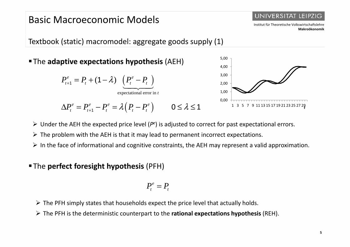
The adaptive expectations hypothesis (AEH)4,00

5,00

( )expectational error in

( )e et t t t

t

P P P Pλ+ = + − −1 1

1,00

2,00

3,00

4,00

Under the AEH the expected price level (Pe) is adjusted to correct for past expectational errors

( )e e e et t t t tP P P P Pλ λ+Δ = − = − ≤ ≤1 0 1

0,001 3 5 7 9 11 13 15 17 19 21 23 25 27 29t

Under the AEH the expected price level (Pe) is adjusted to correct for past expectational errors. The problem with the AEH is that it may lead to permanent incorrect expectations. In the face of informational and cognitive constraints, the AEH may represent a valid approximation.

The perfect foresight hypothesis (PFH)

The PFH simply states that households expect the price level that actually holds.

et tP P=

5

The PFH is the deterministic counterpart to the rational expectations hypothesis (REH).



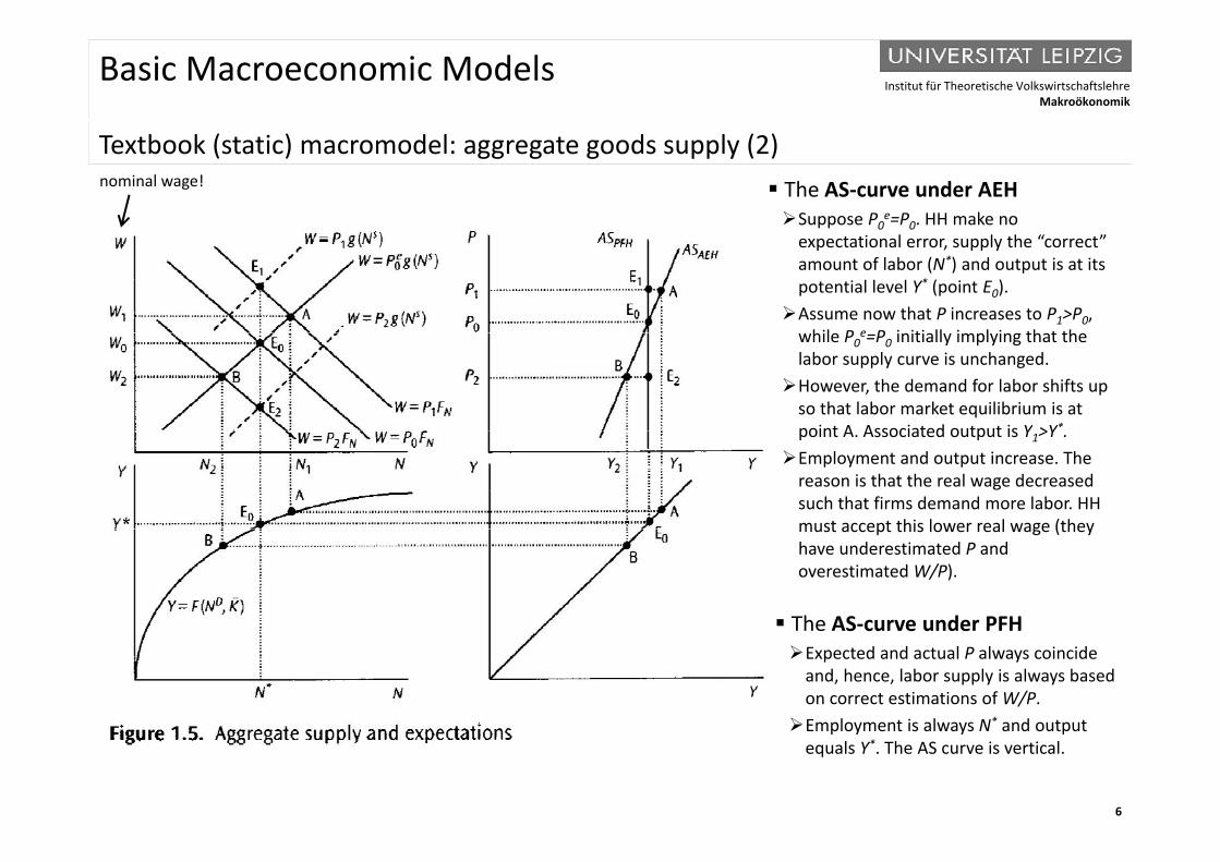
T tb k ( t ti ) d l t d l (2)Textbook (static) macromodel: aggregate goods supply (2) The AS-curve under AEHSuppose P0

e=P0. HH make no i l l h “ ”

nominal wage!

expectational error, supply the “correct” amount of labor (N*) and output is at its potential level Y* (point E0).Assume now that P increases to P1>P0,

hile P e P initiall impl ing that thewhile P0e=P0 initially implying that the

labor supply curve is unchanged. However, the demand for labor shifts up

so that labor market equilibrium is at point A Associated output is Y >Y*point A. Associated output is Y1>Y . Employment and output increase. The

reason is that the real wage decreased such that firms demand more labor. HH must accept this lower real wage (theymust accept this lower real wage (they have underestimated P and overestimated W/P).

The AS-curve under PFHThe AS curve under PFHExpected and actual P always coincide

and, hence, labor supply is always based on correct estimations of W/P.Employment is always N* and output

6

Employment is always N and output equals Y*. The AS curve is vertical.



T tb k ( t ti ) d l t d l (3)Textbook (static) macromodel: aggregate goods supply (3)

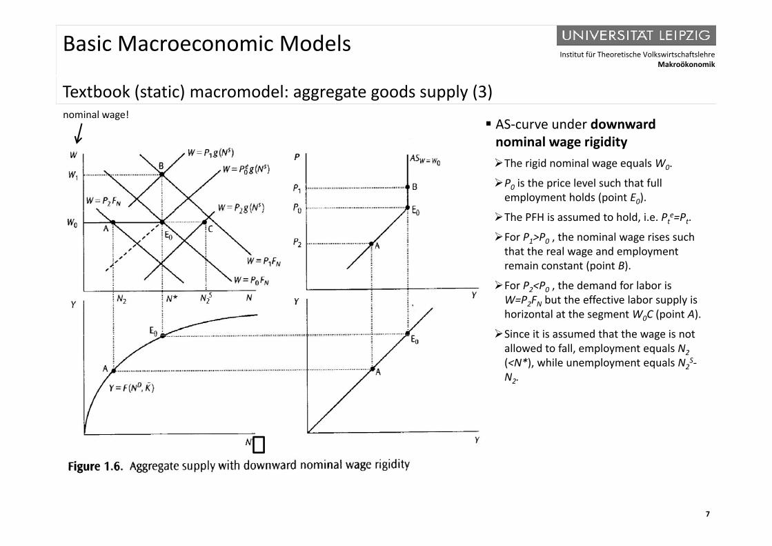
AS-curve under downward nominal wage rigidity

nominal wage!

The rigid nominal wage equals W0.

P0 is the price level such that full employment holds (point E0).

The PFH is assumed to hold, i.e. Pte=Pt.

For P1>P0 , the nominal wage rises such that the real wage and employment remain constant (point B).

For P2<P0 , the demand for labor is W=P2FN but the effective labor supply is horizontal at the segment W0C (point A).

Since it is assumed that the wage is notSince it is assumed that the wage is not allowed to fall, employment equals N2(<N*), while unemployment equals N2

S-N2.

7



T tb k ( t ti ) d l t d d d (1)Textbook (static) macromodel: aggregate goods demand (1)

The demand side of the economy can be described by means of the IS-LM model

t t i

IS : ( ) ( ) ,Y RY C Y T I R G C I= − + + < < ≤ 0 1 0

output=income goods demand

money supply d d

LM : / ( , ) , ,Y RM P L Y R L L= > ≤

0 0

There are two endogenous variables: Y (aggregate demand) and R (interest rate).

money supply money demand

g ( gg g ) ( )

These two equations define Y and R.

U ll th (i ) AD i (Y P) l i ti l l d Usually, the (inverse) AD curve in (Y,P)-plane is negatively sloped.

Provided that LR=-∞ (liquidity trap) and / or IR=0 (investments are insensitive w.r.t. R), the AD curve is vertical in (Y P)-plane (→ goods market equilibrium may not exist)

8

AD curve is vertical in (Y,P) plane (→ goods market equilibrium may not exist).



T tb k ( t ti ) d l t d d d (2)Textbook (static) macromodel: aggregate goods demand (2)

Assume the following specific (linear) functional forms

IS : , ,

LM : / , ,

Y C cY I bR c b

M P kY hR k h

= + + − < < ≥

= − > ≥

0 1 0

0 0

The (inverse) AD-curve then reads

bM

ll h h b l ( ) l ( f l h b h)

[( ) ] ( )bMP

c h bk Y h C I=

− + − +1

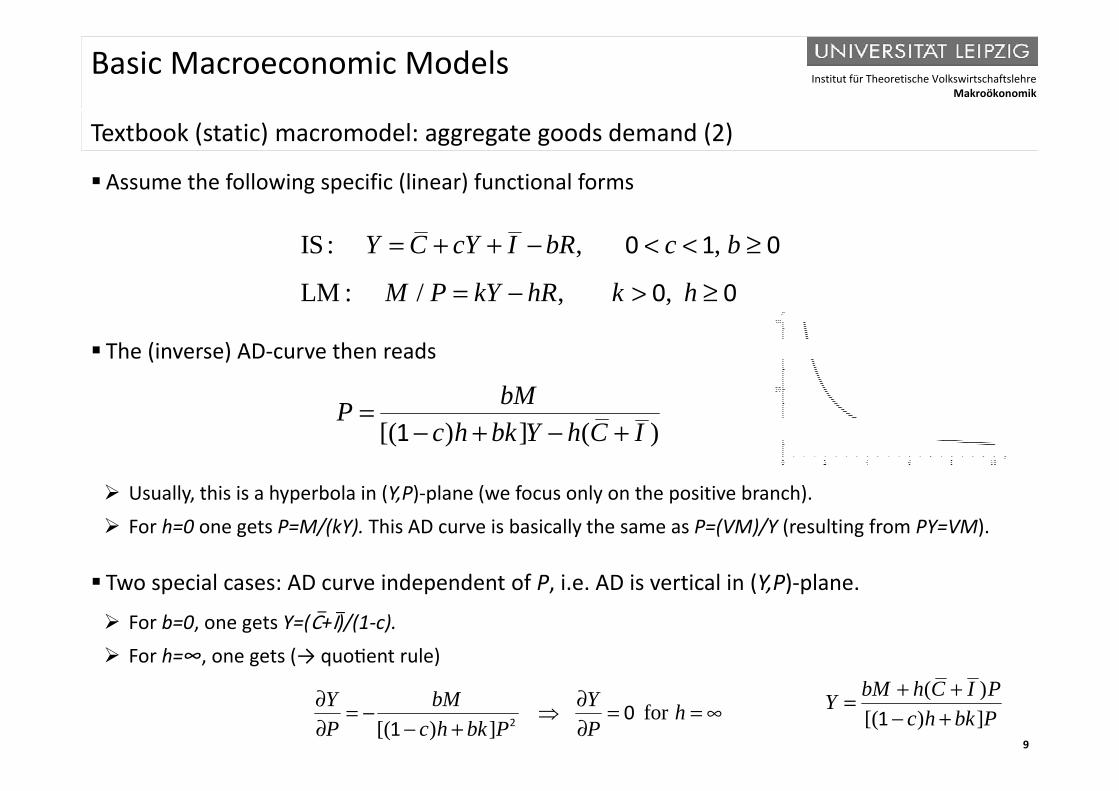
Usually, this is a hyperbola in (Y,P)-plane (we focus only on the positive branch). For h=0 one gets P=M/(kY). This AD curve is basically the same as P=(VM)/Y (resulting from PY=VM).

T i l AD i d d f P i AD i i l i (Y P) l Two special cases: AD curve independent of P, i.e. AD is vertical in (Y,P)-plane.

For b=0, one gets Y=(C+I)/(1-c). For h=∞, one gets (→ quo ent rule)

9

, g ( q )( )

[( ) ]bM h C I PY

c h bk P+ +=

− +1for[( ) ]

Y bM Y hP c h bk P P

∂ ∂= − = = ∞∂ − + ∂2 0

1



D i AS AD d l ADDynamic AS-AD model: AD-curve

The goods market (IS-Curve)

0

0

(1 )( )e

C C b YI I h iY C I G

τπ

= + −

= − −= + +

real interest rate (Fisher-equation)

The money market (LM-Curve)

Y C I G= + +For technical reasons we assume that the demand for real money balances is non-linear.

ln ( )

ln ln ln ( )

kY qid d

s s

M kY qi M eMM M P MP

−= − ⇔ =

= − ⇔ =

The AD-Curveln lns d

PM M=

( )0 0 ln1 (1 )

eh Mq P

h k

C I G hY

bπ

τ ⋅

+ + + ⋅ + ⋅=

− − +

0 00

1

:1 (1 )

/:1 (1 )

h kq

h k

C I Gab

h qab

τ

τ

⋅

⋅

+ +=− − +

=+

10

0 1 2

1 (1 )

(ln ln )

q

e

b

a a M P a

τ

π

+

= + ⋅ − + ⋅ 2

1 (1 )

:1 (1 )

h kq

h kq

b

hab

τ

τ ⋅

− − +

=− − +



D i AS AD d l AS d i fl ti t tiDynamic AS-AD model: AS-curve and inflationary expectations

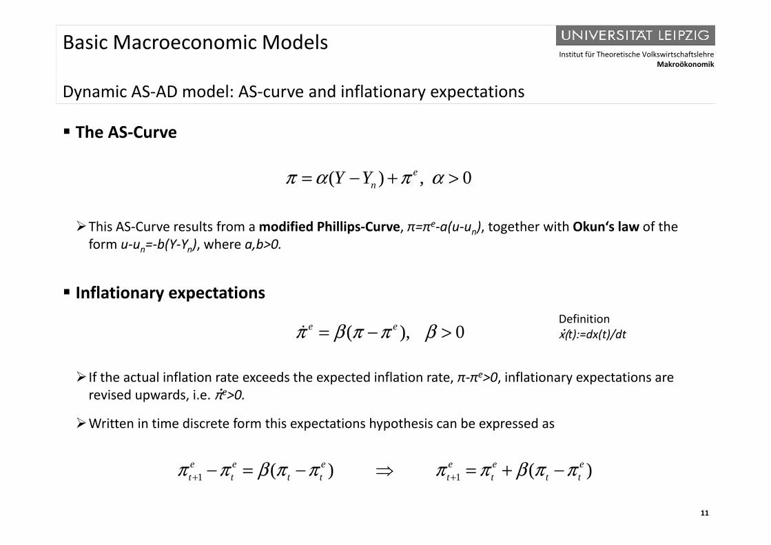
The AS-Curve

( ) , 0enY Yπ α π α= − + >

This AS-Curve results from a modified Phillips-Curve, π=πe-a(u-un), together with Okun‘s law of the form u-un=-b(Y-Yn), where a,b>0.

Inflationary expectations

( ) 0e eπ β π π β= − >Definitionx(t):=dx(t)/dt

If the actual inflation rate exceeds the expected inflation rate, π-πe>0, inflationary expectations are revised upwards i e πe>0

( ), 0π β π π β= > x(t):=dx(t)/dt

revised upwards, i.e. π >0.

Written in time discrete form this expectations hypothesis can be expressed as

11

1 1( ) ( )e e e e e et t t t t t t tπ π β π π π π β π π+ +− = − = + −



D i AS AD d l (3)Dynamic AS-AD model (3)

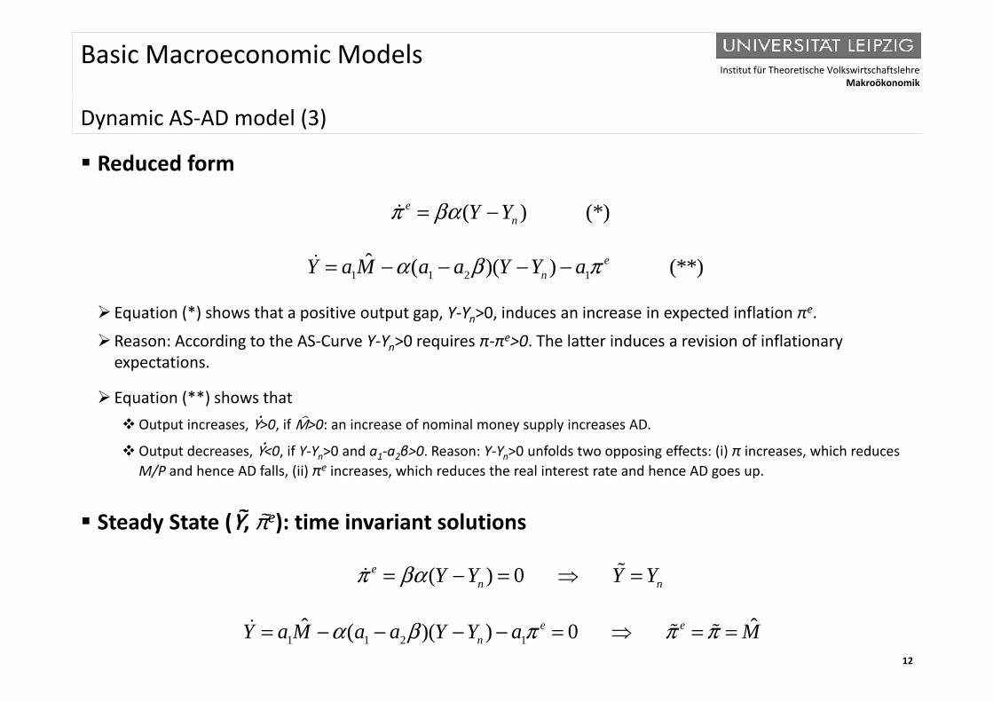
Reduced form

( ) (*)enY Yπ βα= −

1 1 2 1ˆ ( )( ) (**)eY a M a a Y Y aα β π= − − − −

Equation (*) shows that a positive output gap, Y-Yn>0, induces an increase in expected inflation πe.

Reason: According to the AS-Curve Y-Yn>0 requires π-πe>0. The latter induces a revision of inflationary

1 1 2 1( )( ) ( )nY a M a a Y Y aα β π

expectations.

Equation (**) shows that Output increases, Y>0, if M>0: an increase of nominal money supply increases AD.p , , y pp y

Output decreases, Y<0, if Y-Yn>0 and a1-a2β>0. Reason: Y-Yn>0 unfolds two opposing effects: (i) π increases, which reduces M/P and hence AD falls, (ii) πe increases, which reduces the real interest rate and hence AD goes up.

Y Steady State (Y, πe): time invariant solutions

( ) 0en nY Y Y Yπ βα= − = =

12

1 1 2 1ˆ ˆ( )( ) 0e e

nY a M a a Y Y a Mα β π π π= − − − − = = =



D i AS AD d l (3 )Dynamic AS-AD model (3a)

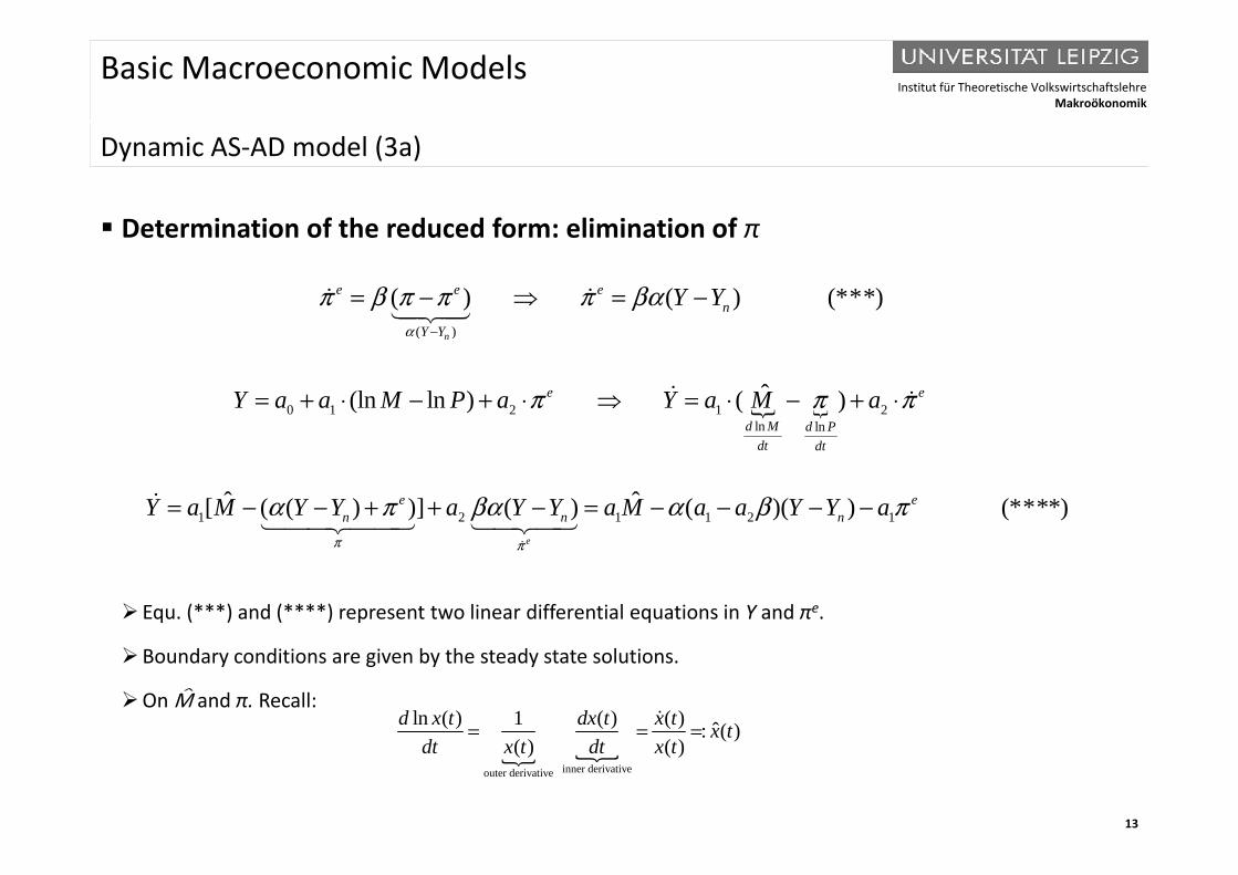
Determination of the reduced form: elimination of π

( )

( ) ( ) (***)n

e e en

Y Y

Y Yα

π β π π π βα−

= − = − ( )n

0 1 2 1 2ln ln

ˆ(ln ln ) ( )e e

d M d P

Y a a M P a Y a M aπ π π= + ⋅ − + ⋅ = ⋅ − + ⋅

dt dt

1 2 1 1 2 1ˆ ˆ[ ( ( ) )] ( ) ( )( ) (****)e e

n n nY a M Y Y a Y Y a M a a Y Y aα π βα α β π= − − + + − = − − − −

Equ. (***) and (****) represent two linear differential equations in Y and πe.

eπ π

Boundary conditions are given by the steady state solutions.

On M and π. Recall: ln ( ) 1 ( ) ( ) ˆ: ( )d x t dx t x t x t= = =

13

inner derivativeouter derivative

: ( )( ) ( )

x tdt x t dt x t



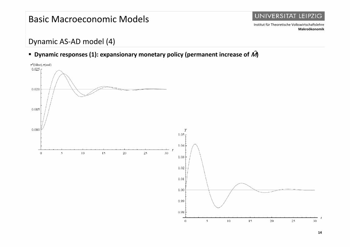
D i AS AD d l (4)Dynamic AS-AD model (4) Dynamic responses (1): expansionary monetary policy (permanent increase of M)

14



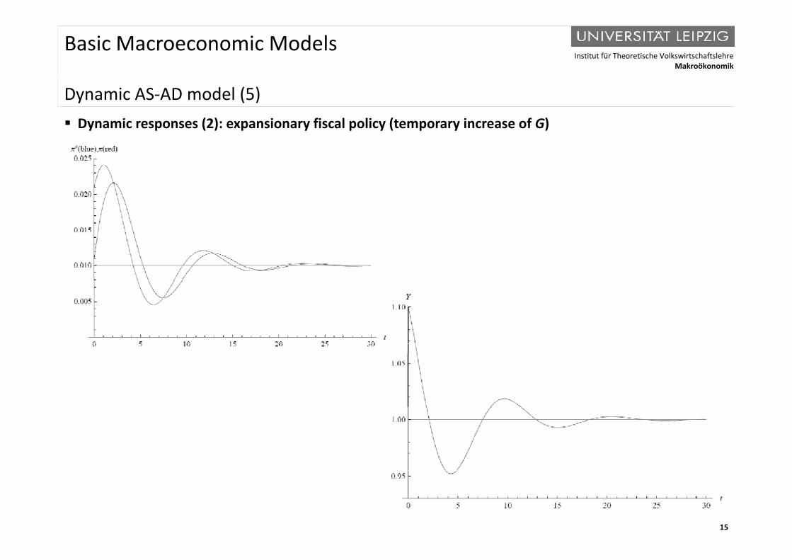
D i AS AD d l (5)Dynamic AS-AD model (5) Dynamic responses (2): expansionary fiscal policy (temporary increase of G)

15



D i AS AD d l (5)Dynamic AS-AD model (5) Dynamic responses (3): negative supply shock (permanent)

16



B i d i d l ith t ti d l t (1)Basic dynamic macromodel with expectations: model setup (1)

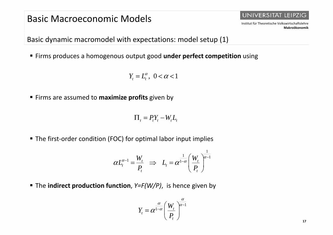
Firms produces a homogenous output good under perfect competition using

, 0 1t tY Lα α= < <

Firms are assumed to maximize profits given by

PY W LΠ =

The first-order condition (FOC) for optimal labor input implies

t t t t tPY W LΠ = −

11 1

1 1t tt t

t t

W WL LP P

αα αα α

−− −

= =

The indirect production function, Y=F(W/P), is hence given by

t t

17

11 t

tt

WYP

αα ααα

−−

=




Labor unions have a target real wage, which is normalized to one, i.e. Wt/Pt=1. Moreover, l b i h th t t W /P 1 H l b i t W ti t d t thlabor unions have the power to set Wt/Pt=1. Hence, labor unions set Wt, negotiated at the beginning of each period t, such that

eW P

There is "substantial unemployment" at Wt/Pt=1. Accordingly, if the real wage falls below one, the additional labor demand by firms can be satisfied

et tW P=

demand by firms can be satisfied. This assumption is compatible with collective bargaining models of unemployment.

The AS-curve can hence be expressed asThe AS curve can hence be expressed as

11 tPY

αα ααα

−−

= t et

YP

α

( )e∗ + Lower case letters denote

18

1 1ln

( )et t ty y a p p

αα

ααα −

=−=

= + − Lower case letters denote (natural) logarithms, i.e. xt:=lnXt.




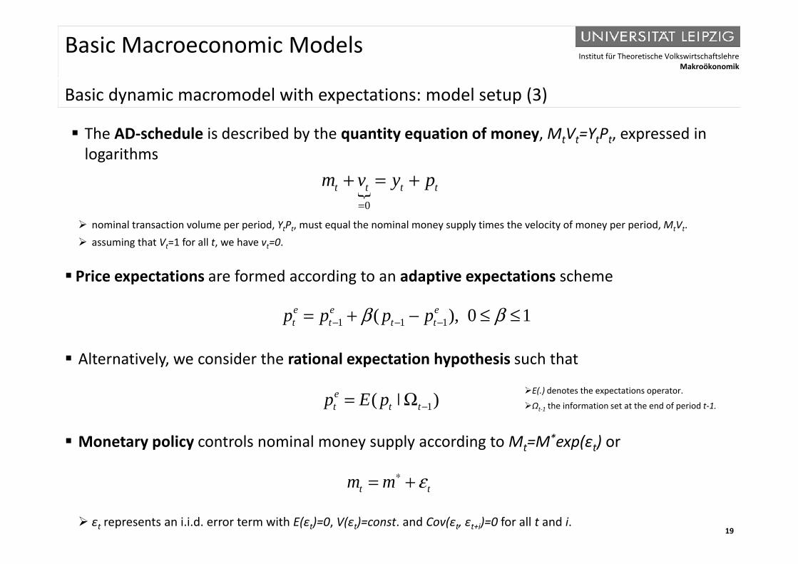
The AD-schedule is described by the quantity equation of money, MtVt=YtPt, expressed in logarithmslogarithms

0

t t t tm v y p=

+ = +

nominal transaction volume per period, YtPt, must equal the nominal money supply times the velocity of money per period, MtVt. assuming that Vt=1 for all t, we have vt=0.

Price expectations are formed according to an adaptive expectations schemep g p p

1 1 1( ), 0 1e e et t t tp p p pβ β− − −= + − ≤ ≤

Alternatively, we consider the rational expectation hypothesis such that

1( )et t tp E p −= Ω E(.) denotes the expectations operator.

Ωt-1 the information set at the end of period t-1.

Monetary policy controls nominal money supply according to Mt=M*exp(εt) or

t 1 p

∗

19 εt represents an i.i.d. error term with E(εt)=0, V(εt)=const. and Cov(εt, εt+i)=0 for all t and i.

t tm m ε∗= +



B i d i d l ith t ti d i t d t d t tBasic dynamic macromodel with expectations: dynamic system and steady state

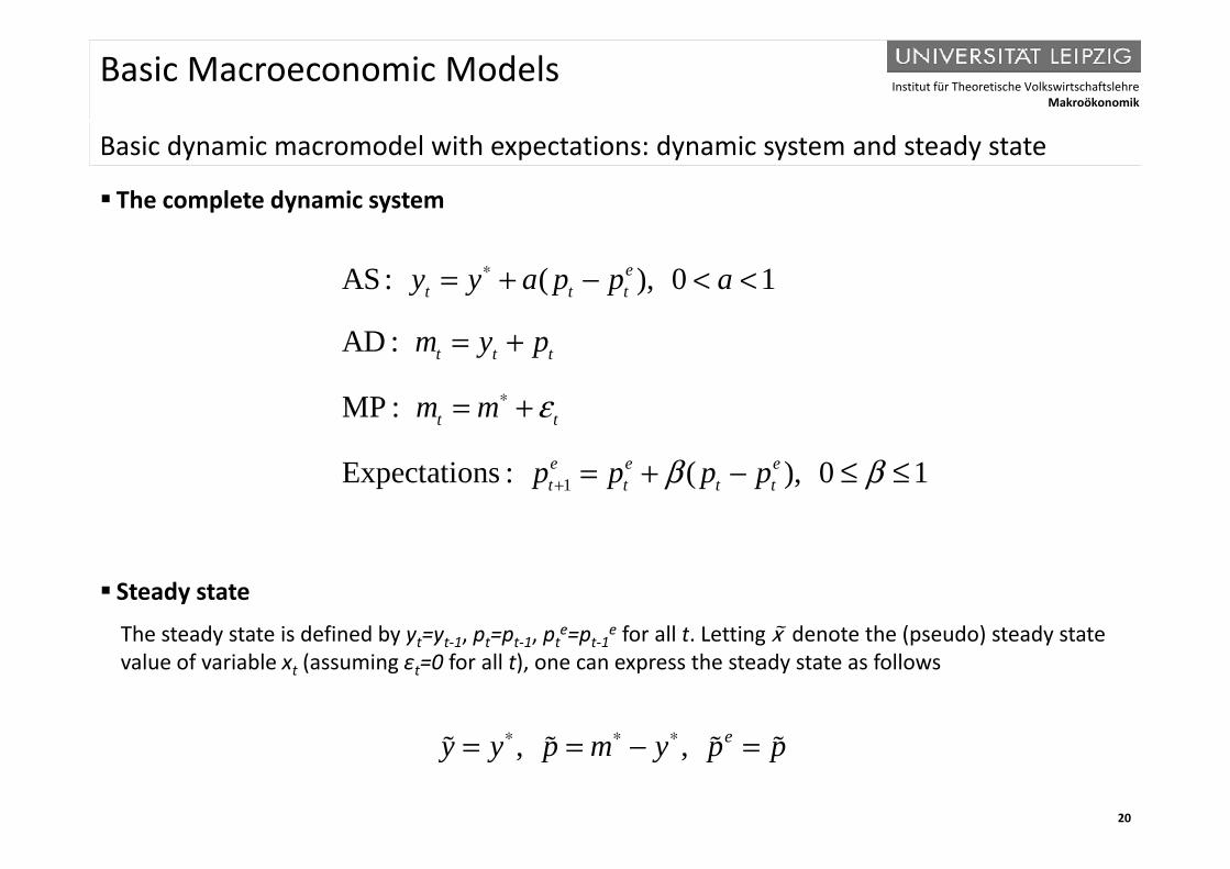
The complete dynamic system

AS: ( ), 0 1

AD

et t ty a p p ay∗= + − < <

+AD :

MP :

t t t

t t

m y p

mm ε∗

= +

= +

1Expectations : ( ), 0 1e e et t t tp p p pβ β+ = + − ≤ ≤

Steady stateThe steady state is defined by y =y p =p p e=p e for all t Letting x denote the (pseudo) steady stateThe steady state is defined by yt=yt-1, pt=pt-1, pt

e=pt-1e for all t. Letting x denote the (pseudo) steady state

value of variable xt (assuming εt=0 for all t), one can express the steady state as follows

20

, , ey y p m y p p∗ ∗ ∗= = − =



B i d i d l ith t ti d d f d i tBasic dynamic macromodel with expectations: reduced-form dynamic system

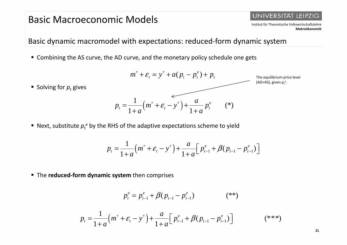
Combining the AS curve, the AD curve, and the monetary policy schedule one gets

Solving for pt gives

( )et t t tm y a p p pε∗ ∗+ = + − + The equilibrium price level

(AD=AS), given pte.

( ) (*)11 1

et t t

ap m y pa a

ε∗ ∗= + − ++ +

Next, substitute pte by the RHS of the adaptive expectations scheme to yield

( ) 1 1 11 ( )e e

t t t t tap m y p p pε β∗ ∗ = + − + + −

The reduced-form dynamic system then comprises

( ) 1 1 1( )1 1t t t t tp m y p p p

a aε β− − − + + + + +

y y p

1 1 1( ) (**)e e et t t tp p p pβ− − −= + −

21

( ) 1 1 11 ( ) (***)

1 1e e

t t t t tap m y p p p

a aε β∗ ∗

− − − = + − + + − + +



B i d i d l ith t ti t li (1)Basic dynamic macromodel with expectations: monetary policy (1)

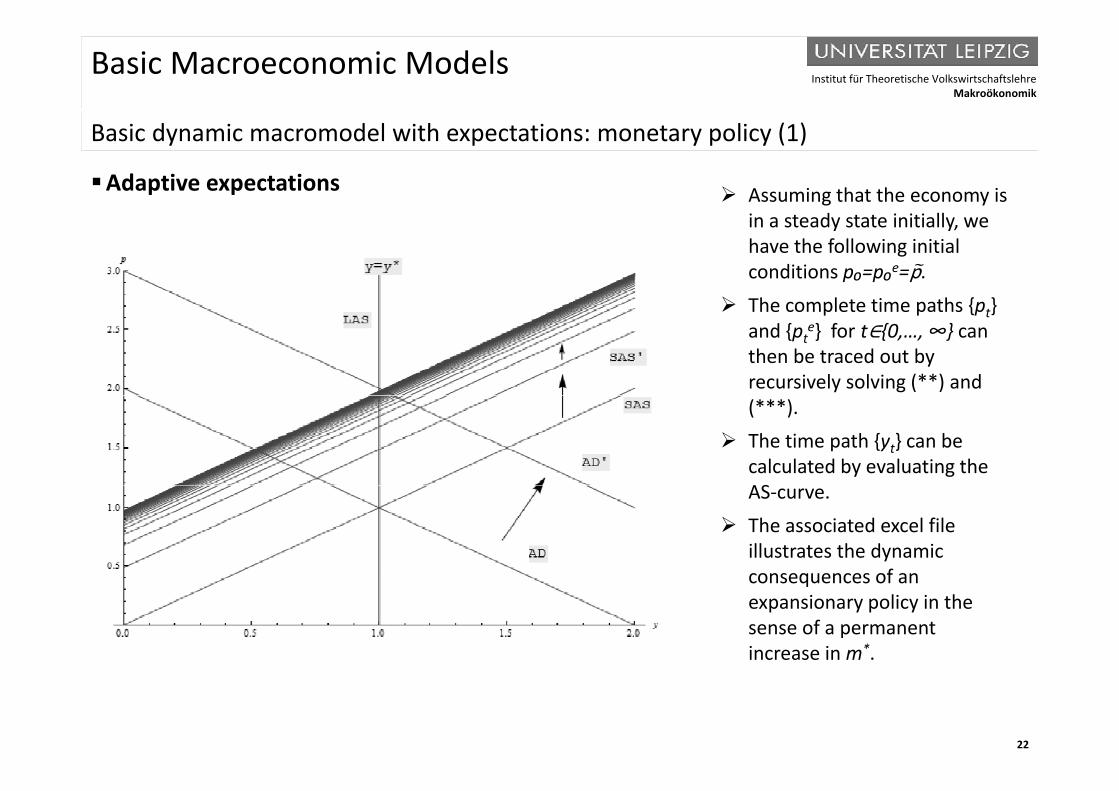
Adaptive expectations Assuming that the economy is i t d t t i iti llin a steady state initially, we have the following initial conditions p₀=p₀e=p.

The complete time paths {p } The complete time paths {pt} and {pt

e} for t∈{0,…, ∞} can then be traced out by recursively solving (**) and (***).

The time path {yt} can be calculated by evaluating the ASAS-curve.

The associated excel file illustrates the dynamic consequences of anconsequences of an expansionary policy in the sense of a permanent increase in m*.

22




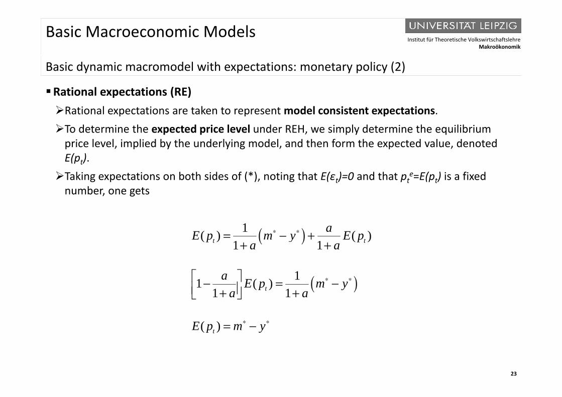
Rational expectations (RE)R ti l t ti t k t t d l i t t t tiRational expectations are taken to represent model consistent expectations.To determine the expected price level under REH, we simply determine the equilibrium

price level, implied by the underlying model, and then form the expected value, denoted ( )E(pt).

Taking expectations on both sides of (*), noting that E(εt)=0 and that pte=E(pt) is a fixed

number, one gets

( )1( ) ( )1 1t t

aE p m y E p∗ ∗= − ++ +

( )

( )

1 1

11 ( )1 1t

a a

a E p m y∗ ∗

+ +

− = − ( )( )

1 1

( )

t

t

p ya a

E p m y∗ ∗

+ +

= −

23




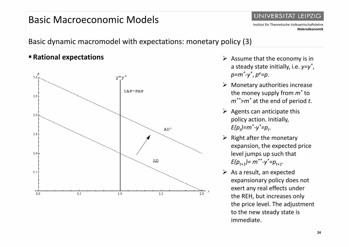
Rational expectations Assume that the economy is in a steady state initially i e y=y*a steady state initially, i.e. y=y , p=m*-y*, pe=p.

Monetary authorities increase the money supply from m* to y pp ym**>m* at the end of period t.

Agents can anticipate this policy action. Initially, E(pt)=m*-y*=pt.

Right after the monetary expansion, the expected price l l j h hlevel jumps up such that E(pt+1)= m**-y*=pt+1.

As a result, an expected expansionary policy does notexpansionary policy does not exert any real effects under the REH, but increases only the price level. The adjustment

24

to the new steady state is immediate.



S h l i M i Cl i l M iSchools in Macroeconomics: Classical Macroeconomics

Demand side: Quantity theory of money implies a demand function like L=kPY. Money demand is not interest sensitive. The velocity of circulation (V=1/k) is constant. The (inverse) AD curve reads: P=M/(kY). The (inverse) AD curve reads: P M/(kY).

Supply side: Strong belief in markets and the efficacy of the price mechanism. Wages and prices are flexible there is perfect foresight Wages and prices are flexible, there is perfect foresight. The labor market clears (at every instant of time), such that N=N*, the AS curve is vertical at Y=Y*. Fiscal and monetary policy cannot affect output and employment.

Policy implications LR=0 implies that the LM-curve is vertical. Expansionary fiscal policy crowds out, via an increase in R, private investment (no shift in AD). Expansionary monetary policy shifts AD, but does not exert any real effects (only P rises).

25



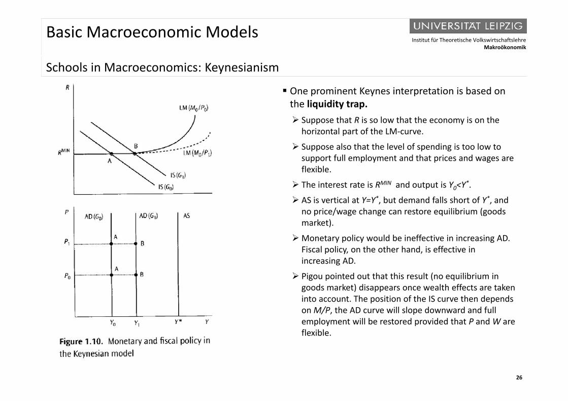
S h l i M i K i iSchools in Macroeconomics: Keynesianism

One prominent Keynes interpretation is based on the liquidity trap. Suppose that R is so low that the economy is on the

horizontal part of the LM-curve.

Suppose also that the level of spending is too low to f ll l d h i dsupport full employment and that prices and wages are

flexible.

The interest rate is RMIN and output is Y0<Y*.

AS is vertical at Y=Y* but demand falls short of Y* and AS is vertical at Y=Y , but demand falls short of Y , and no price/wage change can restore equilibrium (goods market).

Monetary policy would be ineffective in increasing AD. l l h h h d ffFiscal policy, on the other hand, is effective in

increasing AD.

Pigou pointed out that this result (no equilibrium in goods market) disappears once wealth effects are taken g ) ppinto account. The position of the IS curve then depends on M/P, the AD curve will slope downward and full employment will be restored provided that P and W are flexible.

26



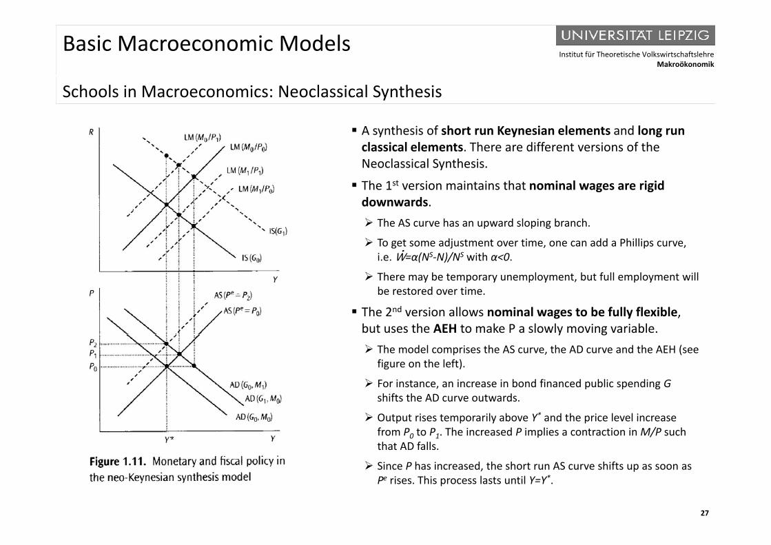
S h l i M i N l i l S th iSchools in Macroeconomics: Neoclassical Synthesis

A synthesis of short run Keynesian elements and long run classical elements There are different versions of theclassical elements. There are different versions of the Neoclassical Synthesis.

The 1st version maintains that nominal wages are rigid downwards. The AS curve has an upward sloping branch.

To get some adjustment over time, one can add a Phillips curve, i.e. W=α(NS-N)/NS with α<0.

h b l b f ll l ll There may be temporary unemployment, but full employment will be restored over time.

The 2nd version allows nominal wages to be fully flexible, but uses the AEH to make P a slowly moving variable. y g The model comprises the AS curve, the AD curve and the AEH (see

figure on the left).

For instance, an increase in bond financed public spending G shifts the AD curve outwardsshifts the AD curve outwards.

Output rises temporarily above Y* and the price level increase from P0 to P1. The increased P implies a contraction in M/P such that AD falls.

27

Since P has increased, the short run AS curve shifts up as soon as Pe rises. This process lasts until Y=Y*.



S h l i M i M t iSchools in Macroeconomics: Monetarism

Monetarism: basic “assumptions and tenets”The interest sensitivity of investment is very high (IR≤0 large in absolute value) so that the IS curve is flat. The interest sensitivity of money demand is very low (LR≈0), i.e. money demand looks like, say, L=kPY.Expectations follow the AEH.p

Monetarism: policy implicationsFiscal policy is largely ineffective in increasing AD An increase in G leads to a strong crowding out ofFiscal policy is largely ineffective in increasing AD. An increase in G leads to a strong crowding out of

private investment.Monetary policy may exert real effects: M=kPY implies that dM>0 leads to d(PY)=(1/k)dM>0.The relative importance of real effects dY and nominal effects dP depends on the assumptions madeThe relative importance of real effects, dY, and nominal effects, dP, depends on the assumptions made

about the labor market and the formation of expectations. Under AEH there are temporary effects on real output and employment. Policy makers may be tempted

to use monetary expansion to combat unemployment Policymakers are however not very good atto use monetary expansion to combat unemployment. Policymakers are, however, not very good at timing monetary policy and there are long and variable lags. As a result, monetary policy is likely to accentuate business cycle fluctuations. Hence, Friedman

suggested that the central bank should follow a constant growth rate rule for some monetary aggregate.

28

gg g y gg g



S h l i M i N Cl i l d N K i E iSchools in Macroeconomics: New Classical and New Keynesian Economics

New Classical Economics: basic “assumptions and tenets” Prices and wages are flexible Prices and wages are flexible. Expectations are formed rational. Macroeconomic theory should be based on microeconomic principles.

New Classical Economics: main implicationsNew Classical Economics: main implications The decentralized allocation of resources is efficient and full employment prevails. Observed fluctuations are not caused by nominal rigidities. Instead rational agents respond to (possibly changing)

economic incentives. Policy ineffectiveness proposition (PIP) applies: Either policy makers cannot (strong version of the PIP) or should not

(weak version of the PIP) use countercyclical policy to smooth business cycle fluctuations.

New Keynesian Economics: basic “assumptions and tenets”New Keynesian Economics: basic assumptions and tenets Markets may not be as perfect as classical economics suggests. Early New Keynesians accepted the REH but stressed nominal wage rigidities (e.g., “multi-period wage contracts”). The most recent wave of New Keynesian economics is more micro-based. y The predominance of imperfect competition, coordination failures and credit constraints are stressed.

New Keynesian Economics: main implications The decentralized allocation of resources may be inefficient and full employment may not prevail

29

The decentralized allocation of resources may be inefficient and full employment may not prevail. The PIP is invalidated: The government can and should stabilize the economy, even under REH.



N t ti d bb i tiNotation and abbreviationsNotation

0<c<1 consumption rateV velocity of circulation

p

0<λ<1 constant parameter

b≥0 sensitivity of I w.r.t. R

β>0 sensitivity of I w.r.t. π

W nominal wage

W :=dW/dt rate of change of W per period dtY output

β>0 sensitivity of I w.r.t. π

C consumption

h≥0 sensitivity of L w.r.t. R

I investment

α>0 constant parameter

I investment

K physical capital

k>0 sensitivity of L w.r.t. Y

L money demand

Abbreviations

AD aggregate demand

AEH adaptive expectations hypothesis L money demand

M money

N labor

NS labor supply

AS aggregate supply

IS goods market equilibrium condition

LM money market equilibrium conditionNS labor supply

P price level

Pe expected price level

t t

PFH perfect foresight hypothesis

PIP policy ineffectiveness proposition

REF rational expectations hypothesis

30

τ tax rate

R interest rate

U utility

am ii basic macroeconomic model - wifa.uni-leipzig.de · institut für theoretische...

Documents