algorithm for optimal winner determination in ...sandholm/oralg.aij.pdf · combinatorial auctions...
TRANSCRIPT
Artificial Intelligence 135 (2002) 1–54
Algorithm for optimal winner determination incombinatorial auctions ✩
Tuomas SandholmComputer Science Department, Carnegie Mellon University, 5000 Forbes Avenue, Pittsburgh, PA 15213, USA
Received 9 March 1999; received in revised form 18 September 2000
Abstract
Combinatorial auctions, that is, auctions where bidders can bid on combinations of items, tend tolead to more efficient allocations than traditional auction mechanisms in multi-item auctions wherethe agents’ valuations of the items are not additive. However, determining the winners so as tomaximize revenue is NP-complete. First, we analyze existing approaches for tackling this problem:exhaustive enumeration, dynamic programming, and restricting the allowable combinations. Second,we study the possibility of approximate winner determination, proving inapproximability in thegeneral case, and discussing approximation algorithms for special cases. We then present our searchalgorithm for optimal winner determination. Experiments are shown on several bid distributionswhich we introduce. The algorithm allows combinatorial auctions to scale up to significantly largernumbers of items and bids than prior approaches to optimal winner determination by capitalizing onthe fact that the space of bids is sparsely populated in practice. The algorithm does this by provablysufficient selective generation of children in the search tree, by using a secondary search for fast childgeneration, by using heuristics that are admissible and optimized for speed, and by preprocessing thesearch space in four ways. Incremental winner determination and quote computation techniques arepresented.
We show that basic combinatorial auctions only allow bidders to express complementarity ofitems. We then introduce two fully expressive bidding languages, called XOR-bids and OR-of-XORs,with which bidders can express general preferences (both complementarity and substitutability). Thelatter language is more concise. We show how these languages enable the use of the Vickrey–Clarke–Groves mechanism to construct a combinatorial auction where each bidder’s dominant strategy is to
✩ This material was first presented as an invited talk at the 1st International Conference on Information andComputation Economies, Charleston, SC, on 10/28/1998. A technical report version of this paper was circulated1/28/1999 (Washington University in St. Louis, Department of Computer Science WUCS-99-01). A conferenceversion of this paper appeared in the International Joint Conference on Artificial Intelligence (IJCAI), Stockholm,Sweden, July 31–August 6, 1999, pp. 542–547. A brief nontechnical overview of different approaches to winnerdetermination appeared in Decision Support Systems 28 (2000) 165–176.
E-mail address: [email protected] (T. Sandholm).
0004-3702/01/$ – see front matter 2001 Elsevier Science B.V. All rights reserved.PII: S0004-3702(01)0 01 59 -X
2 T. Sandholm / Artificial Intelligence 135 (2002) 1–54
bid truthfully. Finally, we extend our search algorithm and preprocessors to handle these languagesas well as arbitrary XOR-constraints between bids. 2001 Elsevier Science B.V. All rights reserved.
Keywords: Auction; Combinatorial auction; Multi-item auction; Multi-object auction; Bidding with synergies;Winner determination; Multiagent systems
1. Introduction
Auctions are popular, distributed and autonomy-preserving ways of allocating items(goods, resources, services, etc.) among agents. They are relatively efficient both in termsof process and outcome. They are extensively used among human bidders in a variety oftask and resource allocation problems. More recently, Internet auction servers have beenbuilt that allow software agents to participate in the auctions as well [61], and some ofthese auction servers even have built-in support for mobile agents [47].
In an auction, the seller wants to sell the items and get the highest possible payments forthem while each bidder wants to acquire the items at the lowest possible price. Auctionscan be used among cooperative agents, but they also work in open systems consistingof self-interested agents. An auction can be analyzed using noncooperative game theory:what strategies are self-interested agents best off using in the auction (and therefore willuse), and will a desirable social outcome—for example, efficient allocation—still follow.Auction mechanisms can be designed so that desirable social outcomes follow even thougheach agent acts based on self-interest.
This paper focuses on auctions with multiple distinguishable items to be allocated,but the techniques could also be used in the special case where some of the items areindistinguishable. These auctions are complex in the general case where the bidders havepreferences over bundles, that is, a bidder’s valuation for a bundle of items need not equalthe sum of his valuations of the individual items in the bundle. This is often the case,for example, in electricity markets, equities trading, bandwidth auctions [34,35], marketsfor trucking services [43,44,48], pollution right auctions, auctions for airport landingslots [40], and auctions for carrier-of-last-resort responsibilities for universal services [27].There are several types of auction mechanisms that could be used in this setting, as thefollowing subsections will discuss.
1.1. Sequential auction mechanisms
In a sequential auction, the items are auctioned one at a time [5,23,48]. Determiningthe winners in such an auction is easy because that can be done by picking the highestbidder for each item separately. However, bidding in a sequential auction is difficult if thebidders have preferences over bundles. To determine her valuation for an item, the bidderneeds to estimate what items she will receive in later auctions. This requires speculationon what the others will bid in the future because that affects what items she will receive.Furthermore, what the others bid in the future depends on what they believe others will bid,etc. This counterspeculation introduces computational cost and other wasteful overhead.Moreover, in auctions with a reasonable number of items, such lookahead in the game
T. Sandholm / Artificial Intelligence 135 (2002) 1–54 3
tree is intractable, and then there is no known way to bid rationally. Bidding rationallywould involve optimally trading off the computational cost of lookahead against the gainsit provides, but that would again depend on how others strike that tradeoff. Furthermore,even if lookahead were computationally manageable, usually uncertainty remains aboutthe others’ bids because agents do not have exact information about each other. This oftenleads to inefficient allocations where bidders fail to get the combinations they want and getones they do not.
1.2. Parallel auction mechanisms
As an alternative to sequential auctions, a parallel auction design can be used [23,36].In a parallel auction the items are open for auction simultaneously, bidders may placetheir bids during a certain time period, and the bids are publicly observable. This has theadvantage that the others’ bids partially signal to the bidder what the others’ bids will endup being so the uncertainty and the need for lookahead is not as drastic as in a sequentialauction. However, the same problems prevail as in sequential auctions, albeit in a mitigatedform.
In parallel auctions, an additional difficulty arises: each bidder would like to wait untilthe end to see what the going prices will be, and to optimize her bids so as to maximizepayoff given the final prices. Because every bidder would want to wait, there is a chancethat no bidding would commence. As a patch to this problem, activity rules have beenused [34]. Each bidder has to bid at least a certain volume (sum of her bid prices) bypredefined time points in the auction, otherwise the bidder’s future rights are reducedin some prespecified manner (for example, the bidder may be barred from the auction).Unfortunately, the game-theoretic equilibrium bidding strategies in such auctions are notknown. It follows that the outcomes of such auctions are unknown for rational bidders.
1.3. Methods for fixing inefficient allocations
In sequential and parallel auctions, the computational cost of lookahead and counter-speculation cannot be recovered, but one can attempt to fix the inefficient allocations thatstem from the uncertainties discussed above.
One such approach is to set up an aftermarket where the bidders can exchange itemsamong themselves after the auction has closed. While this approach can undo someinefficiencies, it may not lead to an economically efficient allocation in general, and evenif it does, that may take an impractically large number of exchanges among the agents [2,3,46].
Another approach is to allow bidders to retract their bids if they do not get thecombinations that they want. For example, in the Federal Communications Commission’sbandwidth auction the bidders were allowed to retract their bids [34]. In case of a retraction,the item was opened for reauction. If the new winning price was lower than the old one,the bidder that retracted the bid had to pay the difference. This guarantees that retractionsdo not decrease the auctioneer’s payoff. However, it exposes the retracting bidder toconsiderable risk because at retraction time she does not know how much the retractionwill end up costing her.

4 T. Sandholm / Artificial Intelligence 135 (2002) 1–54
This risk can be mitigated by using a leveled commitment mechanism [50,51], wherethe decommitting penalties are set up front, possibly on a per item basis. This mechanismallows the bidders to decommit but it also allows the auctioneer to decommit. A biddermay want to decommit, for example, if she did not get the combination that she wantedbut only a subset of it. The auctioneer may want to decommit, for example, if he believesthat he can get a higher price for the item from someone else. The leveled commitmentmechanism has interesting strategic aspects: the agents do not decommit truthfully becausethere is a chance that the other agent will decommit, in which case the former agentis freed from the contract obligations, does not have to pay the decommitment penalty,and will collect a penalty from the latter agent. We showed that despite such strategicbreach, in Nash equilibrium, the mechanism can increase the expected payoff of bothparties and enable contracts which would not be individually rational to both partiesvia any full commitment contract [45,51]. We also developed algorithms for computingthe Nash equilibrium decommitting strategies and algorithms for optimizing the contractparameters [52]. In addition, we experimentally studied sequences of leveled commitmentcontracts and the associated cascade effects [1,4].
Yet another approach would be to sell options for decommitting, where the price of theoption is paid up front whether or not the option is exercised.
Each one of these methods can be used to implement bid retraction before and/or afterthe winning bids have been determined. While these methods can be used to try to fixinefficient allocations, it would clearly be desirable to get efficient allocations right away inthe auction itself so no fixing would be necessary. Combinatorial auctions hold significantpromise toward this goal.
1.4. Combinatorial auction mechanisms
Combinatorial auctions can be used to overcome the need for lookahead and theinefficiencies that stem from the related uncertainties [14,35,40,43,44]. In a combinatorialauction, there is one seller (or several sellers acting in concert) and multiple bidders. 1
The bidders may place bids on combinations of items. This allows a bidder to expresscomplementarities between items so she does not have to speculate into an item’svaluation the impact of possibly getting other, complementary items. For example, theFederal Communications Commission sees the desirability of combinatorial bidding intheir bandwidth auctions, but so far combinatorial bidding has not been allowed—largelydue to perceived intractability of winner determination. 2 This paper focuses on winnerdetermination in combinatorial auctions where each bidder can bid on combinations (thatis, bundles) of indivisible items, and any number of her bids can be accepted.
1 Combinatorial auctions can be generalized to combinatorial exchanges where there are multiple sellers andmultiple buyers [47,53,57].
2 Also, the Commission was directed by Congress in the 1997 Balanced Budget Act to develop a combinatorialbidding system. Specifically, the Balanced Budget Act requires the Commission to “ . . . directly or bycontract, provide for the design and conduct (for purposes of testing) of competitive bidding using a contingentcombinatorial bidding system that permits prospective bidders to bid on combinations or groups of licenses in asingle bid and to enter multiple alternative bids within a single bidding round” [59].
T. Sandholm / Artificial Intelligence 135 (2002) 1–54 5
The rest of the paper is organized as follows. Section 2 defines the winner determinationproblem formally, analyzes its complexity, and discusses different approaches to attackingit. Section 3 presents our new optimal algorithm for this problem. Section 4 discusses thesetup of our winner determination experiments, and Section 5 discusses the experimen-tal results. Section 6 discusses incremental winner determination and quote computationas well as properties of quotes. Section 7 discusses other applications for the algorithm.Section 8 overviews related tree search algorithms. Section 9 discusses substitutability, in-troduces bidding languages to handle it, and develops an algorithm for determining winnersunder those languages. Section 10 presents conclusions and future research directions.
2. Winner determination in combinatorial auctions
We assume that the auctioneer determines the winners—that is, decides which bidsare winning and which are losing—so as to maximize the seller’s revenue. Such winnerdetermination is easy in non-combinatorial auctions. It can be done by picking the highestbidder for each item separately. This takes O(am) time where a is the number of bidders,and m is the number of items.
Unfortunately, winner determination in combinatorial auctions is hard. LetM be the setof items to be auctioned, and let m= |M|. Then any agent, i , can place a bid, bi(S) > 0,for any combination S ⊆M . We define the length of a bid to be the number of items in thebid.
Clearly, if several bids have been submitted on the same combination of items, forwinner determination purposes we can simply keep the bid with the highest price, andthe others can be discarded as irrelevant since it can never be beneficial for the seller toaccept one of these inferior bids. 3 The highest bid price for a combination is
b(S)= maxi∈ bidders
bi(S). (1)
If agent i has not submitted a bid on combination S, we say bi(S)= 0. 4 So, if no bidderhas submitted a bid on combination S, then we say b(S)= 0. 5
Winner determination in a combinatorial auction is the following problem. The goal isto find a solution that maximizes the auctioneer’s revenue given that each winning bidderpays the prices of her winning bids:
maxW∈A
∑S∈W
b(S) (2)
where W is a partition.
3 Ties in the maximization can be broken in any desired way—for example, randomly or by preferring bidsthat are received earlier over ones received later.
4 The assignment bi (S)= 0 need not actually be carried out as long as special care is taken of the combinationsthat received no bids. As we show later, much of the power of our algorithm stems from not explicitly assigning avalue of zero to combinations that have not received bids, and only constructing those parts of the solution spacethat are actually populated by bids.
5 This corresponds to the auctioneer being able to keep items, or analogously, to settings where disposal ofitems is free.
6 T. Sandholm / Artificial Intelligence 135 (2002) 1–54
Definition 2.1. A partition is a set of subsets of items so that each item is included in atmost one of the subsets. Formally, let S = {S ⊆M}. Then the set of partitions is
A= {W ⊆ S | S,S′ ∈W ⇒ S ∩ S′ = ∅}. (3)
Note that in a partition W , some of the items might not be included in any one of thesubsets S ∈W .
We use this notion of a partition for simplicity. It does not explicitly state who the subsetsof items should go to. However, given an partition W , it is trivial to determine which bidsare winning and which are not: every combination S ∈ W is given to the bidder who placedthe highest bid for S. So, a bidder can win more than one combination.
The winner determination problem can also be formulated as an integer programmingproblem where the decision variable xS = 1 if the (highest) bid for combination S is chosento be winning, and xS = 0 if not. Formally:
max�x
∑S∈S
b(S)xS ∀S ∈ S: xS ∈ {0,1} and ∀i ∈M:∑S|i∈S
xS � 1. (4)
The following subsections discuss different approaches to tackling the winner determi-nation problem.
2.1. Enumeration of exhaustive partitions of items
One way to optimally solve the winner determination problem is to enumerate allexhaustive partitions of items.
Definition 2.2. An exhaustive partition is a partition where each item is included in exactlyone subset of the partition.
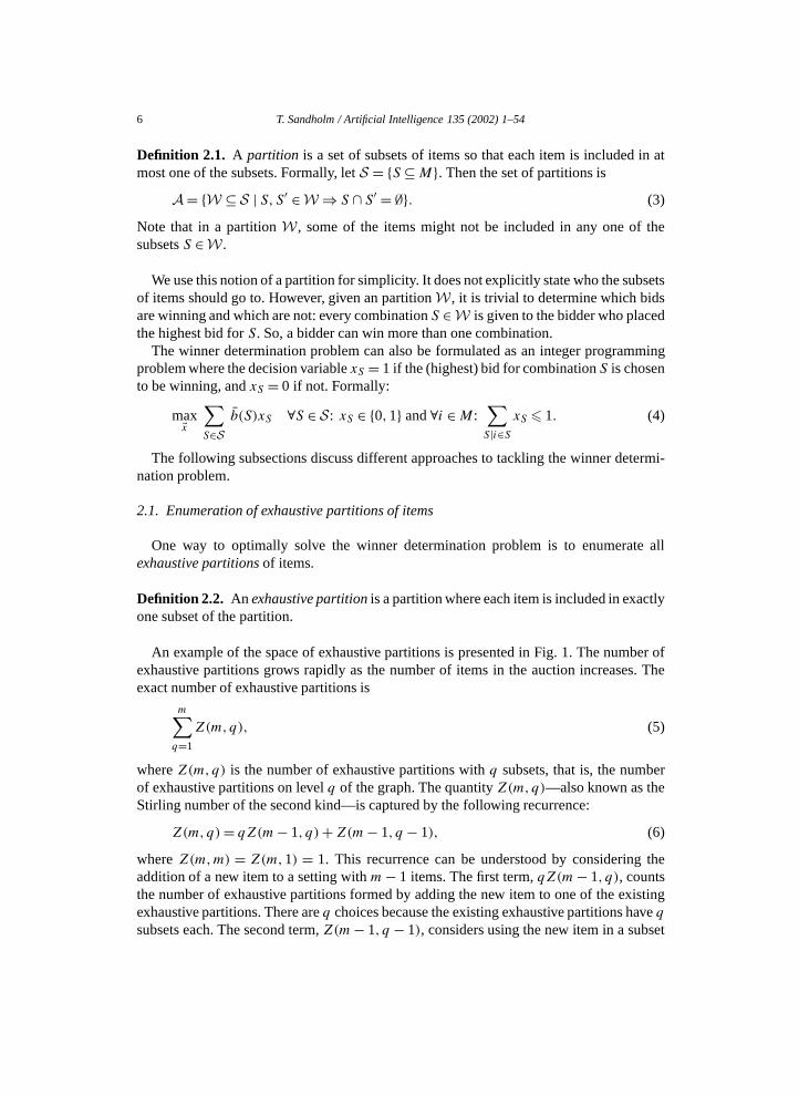
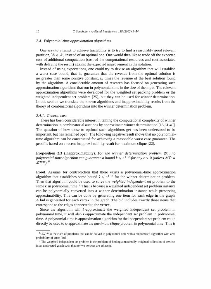
An example of the space of exhaustive partitions is presented in Fig. 1. The number ofexhaustive partitions grows rapidly as the number of items in the auction increases. Theexact number of exhaustive partitions is
m∑q=1
Z(m,q), (5)
where Z(m,q) is the number of exhaustive partitions with q subsets, that is, the numberof exhaustive partitions on level q of the graph. The quantity Z(m,q)—also known as theStirling number of the second kind—is captured by the following recurrence:
Z(m,q)= qZ(m− 1, q)+Z(m− 1, q − 1), (6)
where Z(m,m) = Z(m,1) = 1. This recurrence can be understood by considering theaddition of a new item to a setting with m− 1 items. The first term, qZ(m− 1, q), countsthe number of exhaustive partitions formed by adding the new item to one of the existingexhaustive partitions. There are q choices because the existing exhaustive partitions have qsubsets each. The second term, Z(m− 1, q − 1), considers using the new item in a subset
T. Sandholm / Artificial Intelligence 135 (2002) 1–54 7
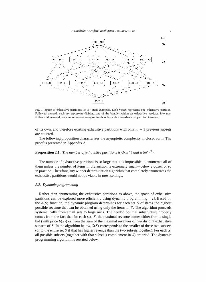
Fig. 1. Space of exhaustive partitions (in a 4-item example). Each vertex represents one exhaustive partition.Followed upward, each arc represents dividing one of the bundles within an exhaustive partition into two.Followed downward, each arc represents merging two bundles within an exhaustive partition into one.
of its own, and therefore existing exhaustive partitions with only m− 1 previous subsetsare counted.
The following proposition characterizes the asymptotic complexity in closed form. Theproof is presented in Appendix A.
Proposition 2.1. The number of exhaustive partitions is O(mm) and ω(mm/2).
The number of exhaustive partitions is so large that it is impossible to enumerate all ofthem unless the number of items in the auction is extremely small—below a dozen or soin practice. Therefore, any winner determination algorithm that completely enumerates theexhaustive partitions would not be viable in most settings.
2.2. Dynamic programming
Rather than enumerating the exhaustive partitions as above, the space of exhaustivepartitions can be explored more efficiently using dynamic programming [42]. Based onthe b(S) function, the dynamic program determines for each set S of items the highestpossible revenue that can be obtained using only the items in S. The algorithm proceedssystematically from small sets to large ones. The needed optimal substructure propertycomes from the fact that for each set, S, the maximal revenue comes either from a singlebid (with price b(S)) or from the sum of the maximal revenues of two disjoint exhaustivesubsets of S. In the algorithm below, C(S) corresponds to the smaller of these two subsets(or to the entire set S if that has higher revenue than the two subsets together). For each S,all possible subsets (together with that subset’s complement in S) are tried. The dynamicprogramming algorithm is restated below.
8 T. Sandholm / Artificial Intelligence 135 (2002) 1–54
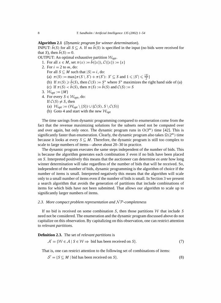
Algorithm 2.1 (Dynamic program for winner determination).INPUT: b(S) for all S ⊆ A. If no b(S) is specified in the input (no bids were received forthat S), then b(S)= 0.OUTPUT: An optimal exhaustive partition Wopt.
1. For all x ∈M , set π(x) := b({x}), C({x}) := {x}2. For i = 2 to m, do:
For all S ⊆M such that |S| = i , do:(a) π(S) := max{π(S \ S′)+ π(S′): S′ ⊆ S and 1 � |S′| � |S|
2 }(b) If π(S)� b(S), then C(S) := S∗ where S∗ maximizes the right hand side of (a)(c) If π(S) < b(S), then π(S) := b(S) and C(S) := S
3. Wopt := {M}4. For every S ∈Wopt, do:
If C(S) �= S, then(a) Wopt := (Wopt \ {S})∪ {C(S), S \ C(S)}(b) Goto 4 and start with the new Wopt
The time savings from dynamic programming compared to enumeration come from thefact that the revenue maximizing solutions for the subsets need not be computed overand over again, but only once. The dynamic program runs in O(3m) time [42]. This issignificantly faster than enumeration. Clearly, the dynamic program also takes �(2m) timebecause it looks at every S ⊆M . Therefore, the dynamic program is still too complex toscale to large numbers of items—above about 20–30 in practice.
The dynamic program executes the same steps independent of the number of bids. Thisis because the algorithm generates each combination S even if no bids have been placedon S. Interpreted positively this means that the auctioneer can determine ex ante how longwinner determination will take regardless of the number of bids that will be received. So,independent of the number of bids, dynamic programming is the algorithm of choice if thenumber of items is small. Interpreted negatively this means that the algorithm will scaleonly to a small number of items even if the number of bids is small. In Section 3 we presenta search algorithm that avoids the generation of partitions that include combinations ofitems for which bids have not been submitted. That allows our algorithm to scale up tosignificantly larger numbers of items.
2.3. More compact problem representation and NP-completeness
If no bid is received on some combination S, then those partitions W that include Sneed not be considered. The enumeration and the dynamic program discussed above do notcapitalize on this observation. By capitalizing on this observation, one can restrict attentionto relevant partitions.
Definition 2.3. The set of relevant partitions is
A′ = {W ∈A | S ∈ W ⇒ bid has been received on S}. (7)
That is, one can restrict attention to the following set of combinations of items:
S ′ = {S ⊆M | bid has been received on S}. (8)
T. Sandholm / Artificial Intelligence 135 (2002) 1–54 9
Let n= |S ′|. This is the number of relevant bids. Recall that for each combination S thathas received a bid, only the highest bid is relevant; all other bids are discarded.
Now, winner determination can be formulated as the following integer program:
max�x
∑S∈S ′
b(S)xS ∀S ∈ S ′: xS ∈ {0,1} and ∀i ∈M:∑S|i∈S
xS � 1. (9)
This integer program has fewer (or an equal number of ) variables and constraints thaninteger program (4) because S ′ ⊆ S . The numbers are the same if and only if everycombination has received a bid.
As discussed above, the complexity of dynamic programming is O(3m). Furthermore,O(3m) = O(2(log2 3)m) = O((2m)log2 3). If each combination of items has received a bid,the input includes O(2m) numbers, which means that the algorithm’s running time,O((2m)log2 3), is polynomial in the size of the input. The following proposition states thegeneral condition under which the dynamic program runs in polynomial time.
Proposition 2.2. If the dynamic program runs in O((n + m)ρ) time for some constantρ > 1, then n ∈ �(2m/ρ). If n ∈ �(2m/ρ) for some constant ρ > 1, then the dynamicprogram runs in O(nρ log2 3) time.
Proof. Since the complexity of the dynamic program f (n,m) ∈ �(2m), there exists aconstant c1 > 0 such that f (n,m) � c12m for large m. If f (n,m) ∈ O((n + m)ρ), thenthere exists a constant c2 > 0 such that f (n,m)� c2(n+m)ρ for large n+m. Therefore,it must be the case that c12m � c2(n+m)ρ . Solving for n we get
n�[c1
c2
(2m
)]1/ρ
−m. (10)
This implies n ∈�(2m/ρ).If n ∈ �(2m/ρ), then there exists a constant c3 > 0 such that n � c32m/ρ for large
m. This means m � ρ(logn − logc3). Since f (n,m) ∈ O(3m), there exists a constantc4 > 0 such that f (n,m)� c43m for large m. Now we can substitute m to get f (n,m)�c43ρ(logn−log c3). Since 3ρ logn = nρ log 3, we get f (n,m) ∈ O(nρ log2 3). ✷
However, the important question is not how complex the dynamic program is, because itexecutes the same steps regardless of what bids have been received. Rather, the importantquestion is whether there exists an algorithm that runs fast in the size of the actual input,which might not include bids on all combinations. In other words, what is the complexityof problem (9)? Unfortunately, no algorithm can, in general, solve it in polynomial timein the size of the input (unless P = NP): the problem is NP-complete [42]. Integerprogramming formulation (9) is the same problem as weighted set packing (once weview each bid as a set (of items) and the price, b(S), as the weight of the set S). NP-completeness of winner determination then follows from the fact that weighted set packingis NP-complete [26].
10 T. Sandholm / Artificial Intelligence 135 (2002) 1–54
2.4. Polynomial-time approximation algorithms
One way to attempt to achieve tractability is to try to find a reasonably good relevantpartition, W ∈ A′, instead of an optimal one. One would then like to trade off the expectedcost of additional computation (cost of the computational resources and cost associatedwith delaying the result) against the expected improvement in the solution.
Instead of using expectations, one could try to devise an algorithm that will establisha worst case bound, that is, guarantee that the revenue from the optimal solution isno greater than some positive constant, k, times the revenue of the best solution foundby the algorithm. A considerable amount of research has focused on generating suchapproximation algorithms that run in polynomial time in the size of the input. The relevantapproximation algorithms were developed for the weighted set packing problem or theweighted independent set problem [25], but they can be used for winner determination.In this section we translate the known algorithms and inapproximability results from thetheory of combinatorial algorithms into the winner determination problem.
2.4.1. General caseThere has been considerable interest in taming the computational complexity of winner
determination in combinatorial auctions by approximate winner determination [15,31,40].The question of how close to optimal such algorithms get has been understood to beimportant, but has remained open. The following negative result shows that no polynomial-time algorithm can be constructed for achieving a reasonable worst case guarantee. Theproof is based on a recent inapproximability result for maximum clique [22].
Proposition 2.3 (Inapproximability). For the winner determination problem (9), nopolynomial-time algorithm can guarantee a bound k � n1−ε for any ε > 0 (unless NP =ZPP). 6
Proof. Assume for contradiction that there exists a polynomial-time approximationalgorithm that establishes some bound k � n1−ε for the winner determination problem.Then that algorithm could be used to solve the weighted independent set problem to thesame k in polynomial time. 7 This is because a weighted independent set problem instancecan be polynomially converted into a winner determination instance while preservingapproximability. This can be done by generating one item for each edge in the graph.A bid is generated for each vertex in the graph. The bid includes exactly those items thatcorrespond to the edges connected to the vertex.
Since the algorithm will k-approximate the weighted independent set problem inpolynomial time, it will also k-approximate the independent set problem in polynomialtime. A polynomial-time k-approximation algorithm for the independent set problem coulddirectly be used to k-approximate the maximum clique problem in polynomial time. This is
6 ZPP is the class of problems that can be solved in polynomial time with a randomized algorithm with zeroprobability of error [38].
7 The weighted independent set problem is the problem of finding a maximally weighted collection of verticesin an undirected graph such that no two vertices are adjacent.

T. Sandholm / Artificial Intelligence 135 (2002) 1–54 11
because the maximum clique problem is the independent set problem on the complementgraph. But Håstad recently showed that no polynomial-time algorithm can establish ak � n1−ε for any ε > 0 for the maximum clique problem (unless NP = ZPP) [22].Contradiction. ✷
From a practical perspective the question of polynomial-time approximation with worstcase guarantees has been answered since algorithms that come very close to the boundof the inapproximability result have been constructed. The asymptotically best algorithmestablishes a bound k ∈ O(n/(logn)2) [19].
One could also ask whether randomized algorithms would help in the winner determina-tion problem. It is conceivable that randomization could provide some improvement overthe k ∈ O(n/(logn)2) bound. However, Proposition 2.3 applies to randomized algorithmsas well, so no meaningful advantage could be gained from randomization.
A bound that depends only on the number of items, m, can be established in polynomialtime. The following algorithm, originally devised by Halldórsson for weighted set packing,establishes a bound k = 2
√m/c [19]. The auctioneer can choose the value for c. As c
increases, the bound improves but the running time increases. Specifically, steps 1 and 2are O((nc )) which is O(nc), step 3 is O(n), step 4 is O(1), step 5 can be naively implementedto be O(m2n2), and step 6 is O(1). So, overall the algorithm is O(max(nc,m2n2)), whichis polynomial for any given c.
Algorithm 2.2 (Greedy winner determination).INPUT: S ′, and b(S) for all S ∈ S ′, and an integer c, 1 � c�m.OUTPUT: An approximately optimal relevant partition Wapprox ∈ A′.
1. A′c := {W ⊆ S ′: S,S′ ∈W ⇒ S ∩ S′ = ∅, |W| � c}
2. W∗c := arg maxW∈A′
c
∑S∈W b(S)
3. S ′′ := {S ∈ S ′: |S| � √m/c}
4. t := 0, S ′′0 := S ′′
5. Repeat(a) t := t + 1(b) Xt := arg maxS∈S ′′
t−1b(S)
(c) Zt := {S ∈ S ′′t−1: Xt ∩ S �= ∅}
(d) S ′′t := S ′′
t−1 −Ztuntil S ′′
t = ∅6. If
∑S∈{X1,X2,...,Xt } b(S) >
∑S∈W∗
cb(S)
then return {X1,X2, . . . ,Xt }else return W∗
c
Another greedy algorithm for winner determination simply inserts bids into theallocation in largest b(S)/
√|S| first order (if the bid shares items with another bidthat is already in the allocation, the bid is discarded) [32]. This algorithm establishes abound k = √
m. If c > 4, the bound that Algorithm 2.2 establishes is better than thatof this algorithm (2
√m/c <
√m). On the other hand, the computational complexity of
Algorithm 2.2 quickly exceeds that of this algorithm as c grows.
12 T. Sandholm / Artificial Intelligence 135 (2002) 1–54
If the number of items is small compared to the number of bids (2√m/c < n or
√m<
n), as will probably be the case in most combinatorial auctions, then these algorithmsestablish a better bound than that of Proposition 2.3. The bound that Algorithm 2.2establishes is about the best that one can obtain: Halldórsson et al. showed (using [22])that a bound k � m1/2−ε cannot be established in polynomial time for any positive ε(unless NP = ZPP) [20]. However, the bound k = m1/2−ε is so high that it is likelyto be of limited value for auctions. Similarly, the bound k = 2
√m/c � 2. Even a bound
k = 2 would mean that the algorithm might only capture 50% of the available revenue. Tosummarize, the approach of constructing polynomial-time approximation algorithms withworst case guarantees seems futile in the general winner determination problem.
2.4.2. Special casesWhile the general winner determination problem (9) is inapproximable in polynomial
time, one can do somewhat better in special cases where the bids have special structure.For example, there might be some cap on the number of items per bid, or there might be acap on the number of bids with which a bid can share items.
The desired special structure could be enforced on the bidders by restricting theallowable bids. However, that can lead to the same inefficiencies as non-combinatorialauctions because bidders may not be allowed to bid on the combinations they want.Alternatively, the auctioneer can allow general bids and use these special case algorithmsif the bids happen to exhibit the desired special structure.
This section reviews the best polynomial-time algorithms for the known special cases.These algorithms were developed for the weighted independent set problem or theweighted set packing problem. Here we show how they apply to the winner determinationproblem:
1. If the bids have at most w items each, a bound k = 2(w + 1)/3 can be establishedin O(nw2∆w) time, where ∆ is the number of bids that any given bid can shareitems with (note that ∆ < n) [6]. First, bids are greedily inserted into the solutionon a highest-price-first basis. Then local search is used to improve the solution, andthis search is terminated after a given number of steps. At each step, one new bidis inserted into the solution, and the old bids that share items with the new bid areremoved from the solution. These improvements are chosen so as to maximize theratio of the new bid’s price divided by the sum of the prices of the old bids that wouldhave to be removed.
2. Several algorithms have been developed for the case where each bid shares itemswith at most ∆ other bids. A bound k = �(∆ + 1)/3� can be established in lineartime in the size of the input by partitioning the set of bids into �(∆+ 1)/3� subsetssuch that ∆ � 2 in each subset, and then using dynamic programming to solve theweighted set packing problem in each subset [18]. Other polynomial-time algorithmsfor this setting establish bounds k =∆/2 [24] and k = (∆+ 2)/3 [21].
3. If the bids can be colored with c colors so that no two bids that share items have thesame color, then a bound k = c/2 can be established in polynomial time [24].
4. The bids have a κ-claw if there is some bid that shares items with κ other bidswhich themselves do not share items. If the bids are free of κ-claws, a bound
T. Sandholm / Artificial Intelligence 135 (2002) 1–54 13
k = κ − 2 + ε can be established with local search in nO(1/ε) time [18]. Anotheralgorithm establishes a bound k = (4κ + 2)/5 in nO(κ) time [18].
5. Let D be the largest d such that there is some subset of bids in which every bidshares items with at least d bids in that subset. Then, a bound k = (D + 1)/2 can beestablished in polynomial time [24].
Approximation algorithms for these known special cases have been improved repeatedly.There is also the possibility that probabilistic algorithms could improve upon thedeterministic ones. In addition, it is possible that additional special cases with desirableapproximability properties will be found. For example, while the current approximationalgorithms are based on restrictions on the structure of bids and items, a new family ofrestrictions that will very likely lend itself to approximation stems from limitations on theprices. For example, if the function b(S) is close to additive, approximation should be easy.Unfortunately it does not seem reasonable for the auctioneer to restrict the bid prices or todiscard outlier bids. Setting an upper bound could reduce the auctioneer’s revenue becausehigher bids would not occur. Setting a lower bound above zero would disable bidders withlower valuations from bidding, and if no bidder has a valuation above the bound, no bidson those combinations would be placed. That can again reduce the auctioneer’s revenue.Although forcing such special structure does therefore not make sense, the auctioneer couldcapitalize on special price structure if such structure happens to be present.
Put together, considerable work has been done on approximation algorithms for specialcases of combinatorial problems, and these algorithms can be used for special cases ofthe winner determination problem. However, the worst case guarantees provided by thecurrent algorithms are so far from optimum that they are of limited importance for auctionsin practice.
2.5. Restricting the combinations to guarantee optimal winner determination inpolynomial time
If even more severe restrictions apply to the bids, winner determination can be carriedout optimally in polynomial time. To capitalize on this idea in practice, the restrictionswould have to be imposed by the auctioneer since they—at least the currently knownones—are so severe that it is unlikely that they would hold by chance. In this sectionwe review the bid restrictions that have been suggested for achieving polynomial winnerdetermination:
1. If the bids have at most 2 items each, the winners can be optimally determined inO(m3) time using an algorithm for maximum-weight matching [42]. The problem isNP-complete if the bids can have 3 items (this can be proven via a reduction from3-set packing).
2. If the bids are of length 1, 2, or greater than m/c, then the winners can be optimallydetermined in O((nlong)
c−1m3) time, where nlong is the number of bids of lengthgreater than m/c [42]. The (nlong)
c−1 factor comes from exhaustively trying allcombinations of c − 1 long bids. Because each long bid uses up a large numberof items, a solution can include at most c− 1 long bids. The m3 factor follows fromsolving the rest of the problem according to case 1 above. This part of the problemuses bids of length 1 and 2 on the items that were not allocated to the long bids.

14 T. Sandholm / Artificial Intelligence 135 (2002) 1–54
Fig. 2. Left: Allowable bids in a tree structure. Right: Interval bids.
3. If the allowable combinations are in a tree structure such that leaves correspondto items and bids can be submitted on any node (internal or leaf ), winners can beoptimally determined in O(m2) time [42]. For example, in Fig. 2 left, a bid on 4 and5 would be allowed while a bid for 5 and 6 would not. In tree structures the winnerscan be optimally determined by propagating information once up the tree. At everynode, the best decision is to accept either a single bid for all the items in that node orthe best solutions in the children of that node.
4. The items can be ordered and it can be required that bids are only placed onconsecutive items [42]. For example, in Fig. 2 right, a bid on 5, 6, 1, and 2 wouldbe allowed while a bid on 5 and 1 would not. Without wrap-around, the winnerscan be optimally determined using dynamic programming. The algorithm starts fromitem 1, then does 1 and 2, then 1, 2, and 3, etc. The needed optimal substructureproperty comes from the fact that the highest revenue that can be achieved fromitems 1,2, . . . , h can be achieved either by picking a bid that has been placed on thatentire combination, or by picking a bid that has been placed on the combinationg, . . . , h and doing what was best for 1, . . . , g − 1 (all choices 1 < g � h aretried). The algorithm runs in O(m2) time. Recently, Sandholm and Suri developeda faster dynamic program for this problem that runs in O(m+ n) time [53]. This isasymptotically the best one can hope for.If wrap-around is allowed, the winners can be optimally determined in O(m3) timeby rerunning the O(m2) algorithm m times, each time cutting the chain at a differentpoint [42]. Using the faster algorithm of Sandholm and Suri for each of these runs,this takes only O(m(n+m)) time [53].
5. One could introduce families of combinations of items where the winner determi-nation is easy within each family, and any two combinations from different familiesintersect. The winner determination problem can then be solved within each familyseparately, and the solution from the family with the highest revenue chosen [42].For example, one could lay the items in a rectangular grid. One family could then becolumns and another family could be rows.
6. One could lay the items in a tree structure, and allow bidding on any subtree. Thiscan be solved in O(nm) time using a dynamic program [53]. The problem becomesNP-complete already if the items are structured in a directed acyclic graph, and bidsare allowed on any directed subtree.
Imposing restrictions on the bids introduces some of the same inefficiencies that arepresent in non-combinatorial auctions because the bidders may be barred from bidding onthe combinations that they want. There is an inherent tradeoff here between computationalspeed and economic efficiency. Imposing certain restrictions on bids achieves provablypolynomial-time winner determination but gives rise to economic inefficiencies.
T. Sandholm / Artificial Intelligence 135 (2002) 1–54 15
3. Our optimal search algorithm
We generated another approach to optimal winner determination. It is based on highlyoptimized search. The motivation behind our approach is to
• allow bidding on all combinations—unlike the approach above that restricts thecombinations. This is in order to avoid all of the inefficiencies that occur in non-combinatorial auctions. Recall that those auctions lead to economic inefficiency andcomputational burden for the bidders that need to look ahead in a game tree andcounterspeculate each other.
• find the optimal solution (given enough time), unlike the approximation algorithms.This maximizes the revenue that the seller can obtain from the bids. Optimal winnerdetermination also enables auction designs where every bidder has incentive to bidtruthfully regardless of how others bid (this will be discussed later in the paper). Thisremoves the bidder’s motivation to counterspeculate and to bid strategically. If thebidders truthfully express their preferences through bids, revenue-maximizing winnerdetermination also maximizes welfare in the system since the goods end up in thehands of the agents that value them the most.
• completely avoid loops and redundant generation of vertices, that are natural concernsfor algorithms that would try to search the graph of exhaustive partitions (Fig. 1)directly. Our algorithm does not search in that space directly, but instead searches ina more fruitful space.
• capitalize heavily on the sparseness of bids—unlike the dynamic program which usesthe same amount of time irrespective of the number of bids. In practice the spaceof bids is likely to be extremely sparsely populated. For example, even if there areonly 100 items to be auctioned, there are 2100 − 1 combinations, and it would takelonger than the life of the universe to bid on all of them even if every person inthe world submitted a bid per second, and these people happened to bid on differentcombinations. 8 Sparseness of bids implies that the relevant partitions are a smallsubset of all partitions. Unlike the dynamic program, our algorithm only searches inthe space of relevant partitions. It follows that the run time of our algorithm dependson the number of bids received, while in the dynamic program it does not.
3.1. Search space (SEARCH1)
We use tree search to achieve these goals. The input (after only the highest bid is keptfor every combination of items for which a bid was received—all other bids are deleted) isa list of bids, one for each S ∈ S ′:
{B1, . . . ,Bn} = {(B1.S,B1.b), . . . , (Bn.S,Bn.b)
}(11)
where Bj .S is the set of items in bid j , and Bj .b is the price in bid j .
8 However, in some settings there might be compact representations that the bidders can make that expand to alarge number of bids. For example, a bidder may state that she is ready to pay $20 for any 5 items in some set S
of items. This would expand to ( |S|5 ) bids.
16 T. Sandholm / Artificial Intelligence 135 (2002) 1–54
Each path in our search tree consists of a sequence of disjoint bids, that is, bids that donot share items with each other (Bj .S ∩ Bk.S = ∅ for all bids j and k on the same path).So, at any point in the search, a path corresponds to a relevant partition.
Let U be the set of items that are already used on the path:
U =⋃
j |Bj is on the path
Bj .S (12)
and let F be the set of free items:
F =M −U. (13)
A path ends when no bid can be added to the path. This occurs when for every bid, someof its items have already been used on the path (∀j,Bj .S ∩U �= ∅).
As the search proceeds down a path, a tally g is kept of the sum of the prices of the bidson the path:
g =∑
j |Bj is on the path
Bj .b. (14)
At every search node, the revenue from the path, that is, the g-value, is compared to thebest g-value found so far in the search tree to determine whether the current solution (path)is the best one so far. If so, it is stored as the best solution found so far. Once the searchcompletes, the stored solution is an optimal solution.
However, care has to be taken to correctly treat the possibility that the auctioneer maybe able to keep items:
Proposition 3.1. The auctioneer’s revenue can increase if she can keep items, that is, ifshe does not have to allocate all items to the bidders. Keeping items increases revenue onlyif there is some item such that no bids (of positive price) have been submitted on that itemalone.
Proof. Consider an auction of two items: 1 and 2. Say there is no bid for item 1, a $5 bidfor item 2, and a $3 bid for the combination of 1 and 2. Then it is more profitable (revenue$5) for the auctioneer to keep 1 and to allocate 2 alone than it would be to allocate both 1and 2 together (revenue $3).
If there are bids of positive price for each item alone, the auctioneer would receive apositive revenue by allocating each item alone to a bidder (regardless of how the auctioneerallocates the other items). Therefore, the auctioneer’s revenue would be strictly lower if hekept items. ✷
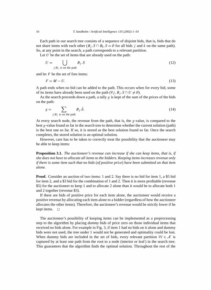
The auctioneer’s possibility of keeping items can be implemented as a preprocessingstep to the algorithm by placing dummy bids of price zero on those individual items thatreceived no bids alone. For example in Fig. 3, if item 1 had no bids on it alone and dummybids were not used, the tree under 1 would not be generated and optimality could be lost.When dummy bids are included in the set of bids, every relevant partition W ∈ A′ iscaptured by at least one path from the root to a node (interior or leaf ) in the search tree.This guarantees that the algorithm finds the optimal solution. Throughout the rest of the
T. Sandholm / Artificial Intelligence 135 (2002) 1–54 17
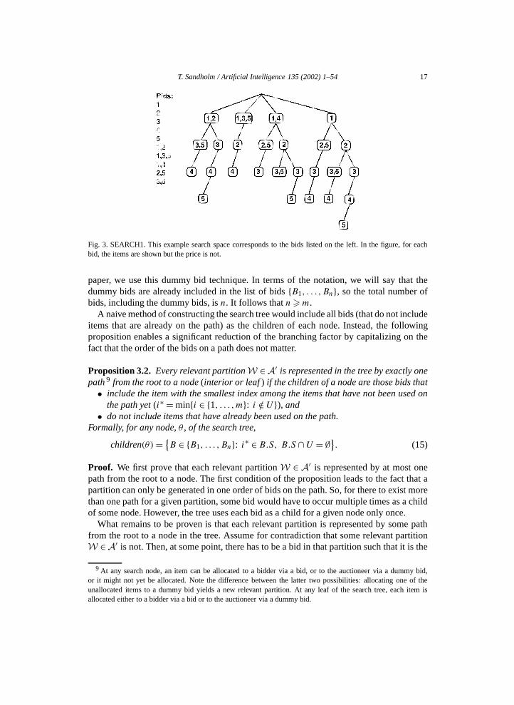
Fig. 3. SEARCH1. This example search space corresponds to the bids listed on the left. In the figure, for eachbid, the items are shown but the price is not.
paper, we use this dummy bid technique. In terms of the notation, we will say that thedummy bids are already included in the list of bids {B1, . . . ,Bn}, so the total number ofbids, including the dummy bids, is n. It follows that n�m.
A naive method of constructing the search tree would include all bids (that do not includeitems that are already on the path) as the children of each node. Instead, the followingproposition enables a significant reduction of the branching factor by capitalizing on thefact that the order of the bids on a path does not matter.
Proposition 3.2. Every relevant partition W ∈A′ is represented in the tree by exactly onepath 9 from the root to a node (interior or leaf ) if the children of a node are those bids that
• include the item with the smallest index among the items that have not been used onthe path yet (i∗ = min{i ∈ {1, . . . ,m}: i /∈U}), and
• do not include items that have already been used on the path.Formally, for any node, θ , of the search tree,
children(θ)= {B ∈ {B1, . . . ,Bn}: i∗ ∈B.S, B.S ∩U = ∅}
. (15)
Proof. We first prove that each relevant partition W ∈ A′ is represented by at most onepath from the root to a node. The first condition of the proposition leads to the fact that apartition can only be generated in one order of bids on the path. So, for there to exist morethan one path for a given partition, some bid would have to occur multiple times as a childof some node. However, the tree uses each bid as a child for a given node only once.
What remains to be proven is that each relevant partition is represented by some pathfrom the root to a node in the tree. Assume for contradiction that some relevant partitionW ∈A′ is not. Then, at some point, there has to be a bid in that partition such that it is the
9 At any search node, an item can be allocated to a bidder via a bid, or to the auctioneer via a dummy bid,or it might not yet be allocated. Note the difference between the latter two possibilities: allocating one of theunallocated items to a dummy bid yields a new relevant partition. At any leaf of the search tree, each item isallocated either to a bidder via a bid or to the auctioneer via a dummy bid.

18 T. Sandholm / Artificial Intelligence 135 (2002) 1–54
bid with the item with the smallest index among those not on the path, but that bid is notinserted to the path. Contradiction. ✷
Our search algorithm restricts the children according to Proposition 3.2. This can beseen, for example, at the first level of Fig. 3 because all the bids considered at the first levelinclude item 1. Fig. 3 also illustrates the fact that the minimal index, i∗, does not coincidewith the depth of the search tree in general.
To summarize, in the search tree, a path from the root to a node (interior or leaf )corresponds to a relevant partition. Each relevant partition W ∈ A′ is represented byexactly one such path. The other partitions W ∈ A − A′ are not generated. We call thissearch SEARCH1.
3.1.1. Size of the tree in SEARCH1In this section we analyze the worst case size of the tree in SEARCH1.
Proposition 3.3. The number of leaves in SEARCH1 is no greater than (n/m)m. Also, thenumber of leaves in SEARCH1 is no greater than
∑mq=1Z(m,q) ∈ O(mm) (see Eqs. (5)
and (6) for the definition of Z). Furthermore, the number of leaves in SEARCH1 is nogreater than 2n.
The number of nodes in SEARCH1 (excluding the root) is no greater than m times thenumber of leaves. The number of nodes in SEARCH1 is no greater than 2n.
Proof. We first prove that the number of leaves is no greater than (n/m)m. The depth ofthe tree is at most m since every node on a path uses up at least one item. Let Ni be the setof bids that include item i but no items with a smaller index than i . Let ni = |Ni |. Clearly,∀i, j, Ni ∩Nj = ∅, so n1 + n2 + · · · + nm = n. An upper bound on the number of leavesin the tree is given by n1 ·n2 · · · · ·nm because the branching factor at a node is at most ni∗ ,and i∗ increases strictly along every path in the tree. The maximization problem
max n1 · n2 · · · · · nm s.t. n1 + n2 + · · · + nm = nis solved by n1 = n2 = · · · = nm = n/m. Even if n is not divisible by m, the value of themaximization is an upper bound. Therefore, the number of leaves in the tree is no greaterthan (n/m)m.
Now we prove that the number of leaves in SEARCH1 is no greater than∑mq=1Z(m,q)∈ O(mm). Since dummy bids are used, each path from the root to a leaf corresponds
to a relevant exhaustive partition. Therefore the number of leaves is no greater than thenumber of exhaustive partitions (and is generally lower since not all exhaustive partitionsare relevant). In Section 2.1 we showed that that the number of exhaustive partitions is∑mq=1Z(m,q). By Proposition 2.1, this is O(mm).Next we prove that the number of nodes (and thus also the number of leaves) is no greater
than 2n. There are 2n combinations of bids (including the one with no bids). In the searchtree, each path from a root to a node corresponds to a unique combination of bids (thereverse is not true because in some combinations bids share items, so those combinationsare not represented by any path in the tree). Therefore, the number of nodes is no greaterthan 2n.
T. Sandholm / Artificial Intelligence 135 (2002) 1–54 19
Because there are at most m nodes on a path (excluding the root), the number of nodesin the tree (excluding the root) is no greater than m times the number of leaves. ✷Proposition 3.4. The bound (n/m)m is always tighter (lower) than the bound 2n.
Proof.(n
m
)m< 2n ⇔ m log
n
m< n ⇔ log
n
m<n
m
which holds for all positive numbers n and m. ✷The bound (n/m)m shows that the number of leaves (and nodes) in SEARCH1 is
polynomial in the number of bids even in the worst case if the number of items is fixed. Onthe other hand, as the number of items increases, the number of bids also increases (n�mdue to dummy bids), so in the worst case, the number of leaves (and nodes) in SEARCH1remains exponential in the number of items m.
3.2. Fast generation of children (SEARCH2)
At any given node, θ , of the tree, SEARCH1 has to determine children(θ). In otherwords, it needs to find those bids that satisfy the two conditions of Proposition 3.2. A naiveapproach is to loop through a list of all bids at every search node, and accept a bid as achild if it includes i∗, and does not include items in U . This takes *(nm) time per searchnode because it loops through the list of bids, and for each bid it loops through the list ofitems. 10
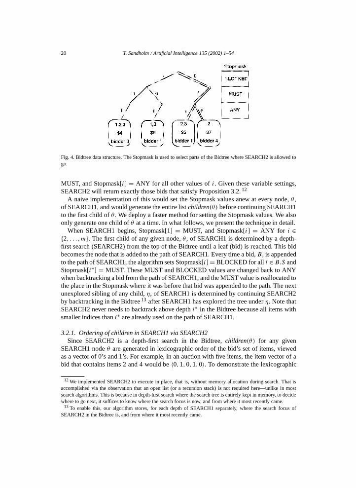
We use a more sophisticated scheme to make child generation faster. Our versionof SEARCH1 uses a secondary depth-first search, SEARCH2, to quickly determine thechildren of a node. SEARCH2 takes place in a different space: a data structure which wecall the Bidtree. It is a binary tree in which the bids are inserted up front as the leaves (onlythose parts of the tree are generated for which bids are received) (Fig. 4).
The use of a Stopmask differentiates the Bidtree from a classic binary tree. The Stopmaskis a vector with one variable for each item, i ∈M . Stopmask[i] can take on any one of threevalues: BLOCKED, MUST, or ANY. If Stopmask[i] = BLOCKED, SEARCH2 will neverprogress left at depth i . 11 This has the effect that those bids that include item i are prunedinstantly and in place. If, instead, Stopmask[i] = MUST, then SEARCH2 cannot progressright at depth i . This has the effect that all other bids except those that include item i arepruned instantly and in place. Stopmask[i] = ANY corresponds to no pruning based onitem i: SEARCH2 may go left or right at depth i . Fig. 4 illustrates how particular values inthe Stopmask prune the Bidtree.
SEARCH2 is used to generate children in SEARCH1. The basic principle is that at anygiven node of SEARCH1, Stopmask[i] = BLOCKED for all i ∈ U , and Stopmask[i∗] =
10 On a k-bit architecture, this time can be reduced by a factor of k by representing B.S as a bitmask of items,and by representing U as a bitmask of items. The machine can then compute B.S XOR U on the bitmasks k bitsat a time. If this does not return 0, then the bid includes items in U .
11 The root of the tree is at depth 1.
20 T. Sandholm / Artificial Intelligence 135 (2002) 1–54
Fig. 4. Bidtree data structure. The Stopmask is used to select parts of the Bidtree where SEARCH2 is allowed togo.
MUST, and Stopmask[i] = ANY for all other values of i . Given these variable settings,SEARCH2 will return exactly those bids that satisfy Proposition 3.2. 12
A naive implementation of this would set the Stopmask values anew at every node, θ ,of SEARCH1, and would generate the entire list children(θ) before continuing SEARCH1to the first child of θ . We deploy a faster method for setting the Stopmask values. We alsoonly generate one child of θ at a time. In what follows, we present the technique in detail.
When SEARCH1 begins, Stopmask[1] = MUST, and Stopmask[i] = ANY for i ∈{2, . . . ,m}. The first child of any given node, θ , of SEARCH1 is determined by a depth-first search (SEARCH2) from the top of the Bidtree until a leaf (bid) is reached. This bidbecomes the node that is added to the path of SEARCH1. Every time a bid, B , is appendedto the path of SEARCH1, the algorithm sets Stopmask[i] = BLOCKED for all i ∈ B.S andStopmask[i∗] = MUST. These MUST and BLOCKED values are changed back to ANYwhen backtracking a bid from the path of SEARCH1, and the MUST value is reallocated tothe place in the Stopmask where it was before that bid was appended to the path. The nextunexplored sibling of any child, η, of SEARCH1 is determined by continuing SEARCH2by backtracking in the Bidtree 13 after SEARCH1 has explored the tree under η. Note thatSEARCH2 never needs to backtrack above depth i∗ in the Bidtree because all items withsmaller indices than i∗ are already used on the path of SEARCH1.
3.2.1. Ordering of children in SEARCH1 via SEARCH2Since SEARCH2 is a depth-first search in the Bidtree, children(θ) for any given
SEARCH1 node θ are generated in lexicographic order of the bid’s set of items, viewedas a vector of 0’s and 1’s. For example, in an auction with five items, the item vector of abid that contains items 2 and 4 would be 〈0,1,0,1,0〉. To demonstrate the lexicographic
12 We implemented SEARCH2 to execute in place, that is, without memory allocation during search. That isaccomplished via the observation that an open list (or a recursion stack) is not required here—unlike in mostsearch algorithms. This is because in depth-first search where the search tree is entirely kept in memory, to decidewhere to go next, it suffices to know where the search focus is now, and from where it most recently came.
13 To enable this, our algorithm stores, for each depth of SEARCH1 separately, where the search focus ofSEARCH2 in the Bidtree is, and from where it most recently came.
T. Sandholm / Artificial Intelligence 135 (2002) 1–54 21
order, let i∗ = 2 for the current θ , and let there be two other bids that include item 2. Lettheir item vectors be
〈0,1,0,1,1〉 and 〈0,1,1,0,0〉.Now, the children of θ would be generated in the following order of item vectors:
〈0,1,1,0,0〉, 〈0,1,0,1,1〉, 〈0,1,0,1,0〉.Since the children are generated—and the subtrees under them explored—one by one, thisorder of generating the children is also the order in which the search branches are explored.One implication of this ordering is that a bid with only one item is always the last child tobe explored (Fig. 3).
Alternatively, one could generate all the children of a SEARCH1 node one after theother using SEARCH2, and store them (for example, in a linked list) before exploring anyof them. This would allow the children to be ordered based on additional considerations.Exploring more promising children first could improve the performance of SEARCH1because good solutions would be found earlier. This has two main advantages. First,if SEARCH1 needs to be terminated before it has completed, a better solution will beavailable. Second, finding good solutions earlier allows more pruning of later search pathsin SEARCH1 based on a bounding technique, discussed later in Section 3.5.
3.2.2. Complexity of SEARCH2As discussed in the beginning of the previous section, the naive approach to generating
children(θ) takes *(nm) time in the worst case. As desired, the use of SEARCH2 togenerate children(θ) reduces this complexity, even in the worst case. For any given θ ,finding the entire set children(θ), one at a time, corresponds to conducting a depth-firstsearch (SEARCH2) in the Bidtree. The complexity of SEARCH2 is no greater than thenumber of edges in the Bidtree times two (to account for backtracks). The followingproposition gives a tight upper bound on the number of edges in the Bidtree.
Proposition 3.5. In a tree that has uniform depth m + 1 (under the convention that theroot is at depth 1), n leaves, and where any node has at most two children (as is the casein SEARCH2), the number of edges is at most
nm− n�logn� + 2 · 2�logn� − 2. (16)
This bound is tight. Under the innocuous assumption that m− logn� c for some constantc > 0, this is
O(n · (m− logn)
). (17)
On the other hand, under the assumption that m− logn < c, this is
O(n). (18)
The proof of Proposition 3.5 is given in Appendix B.While the complexity reduction from using SEARCH2 instead of the naive method is
only moderate in the worst case, in many cases, the complexity reduction is significantlygreater. As an extreme example, in the best case SEARCH2 only takes O(1) time (for
22 T. Sandholm / Artificial Intelligence 135 (2002) 1–54
example, if all bids include item 1 and item 1 is already used on the path), while thecomplexity of the naive approach remains *(nm). Another good case for SEARCH2 is awide-late-tree (Fig. B.1 right), where the upper part has O(m− logn) edges and the lowerpart has O(2logn)= O(n) edges, so the overall complexity is O(max(m− logn,n)).
Also, the analysis in this section pertains to a single SEARCH1 node. Due to substantialpruning using the Stopmask, all nodes in SEARCH1 cannot suffer this worst case inchild generation. Future research should further study the complexity of child generationwhen amortized over all SEARCH1 nodes. As will be discussed later in this paper,some of the SEARCH1 nodes will be pruned. Therefore, a sophisticated analysis ofchild generation would only amortize over those SEARCH1 nodes for which children areactually generated.
3.3. Anytime winner determination: Using a depth-first search strategy for SEARCH1
We first implemented the main search (SEARCH1) as depth-first search. It runs inlinear space (not counting the statically allocated Bidtree data structure that uses slightlymore memory as shown in Proposition 3.5). Feasible solutions are found quickly. The firstrelevant exhaustive partition is found at the end of the first search path (that is, at the left-most leaf ). In fact, even a path from the root to an interior node could be converted into afeasible solution by having the auctioneer keep the items F that have not been allocated onthe path so far.
The solution improves monotonically since our algorithm keeps track of the best solutionfound so far. This implements the anytime feature: if the algorithm does not complete inthe desired amount of time, it can be terminated prematurely, and it guarantees a feasiblesolution that improves monotonically. When testing the anytime feature, it turned outthat in practice most of the revenue was generated early on as desired, and there werediminishing returns to computation.
3.4. Preprocessing
Our algorithm preprocesses the bids in four ways to make the main search faster withoutcompromising optimality. The preprocessors could also be used in conjunction withapproaches to winner determination other than our search algorithm. The next subsectionspresent the preprocessors in the order in which they are executed.
3.4.1. PRE1: Keep only the highest bid for a combinationWhen a bid arrives, it is inserted into the Bidtree. If a bid for the same set of items S
already exists in the Bidtree (that is, the leaf that would have been created for the new bidalready exists), only the bid with the higher price is kept, and the other bid is discarded.Ties can be broken randomly or, for example, in favor of the bid that was received earlier.Inserting a bid into the Bidtree is *(m) because insertion involves following or creatinga path of length m. There are n bids to insert. So, the overall time complexity of PRE1 is*(mn).
T. Sandholm / Artificial Intelligence 135 (2002) 1–54 23
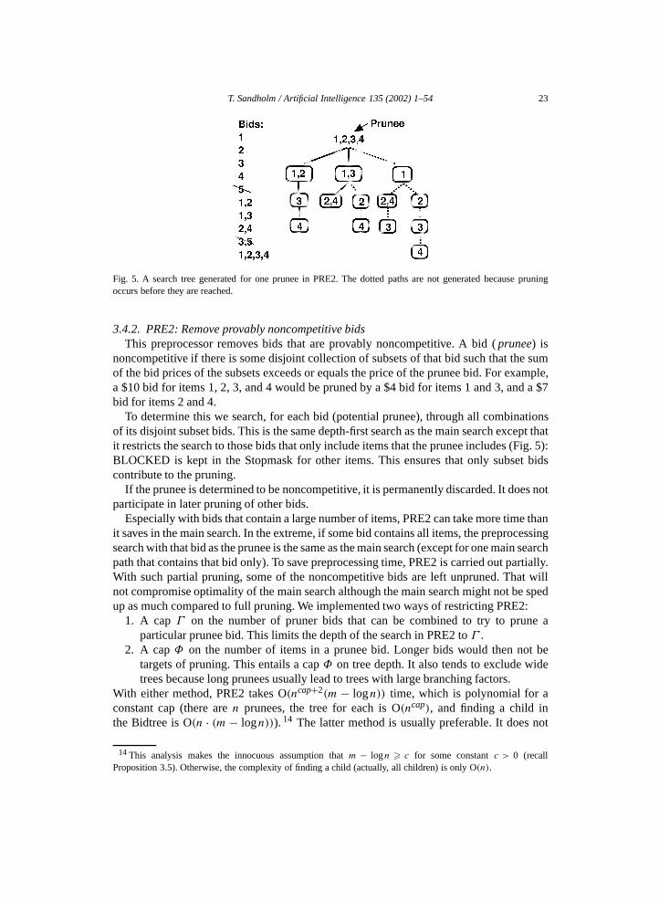
Fig. 5. A search tree generated for one prunee in PRE2. The dotted paths are not generated because pruningoccurs before they are reached.
3.4.2. PRE2: Remove provably noncompetitive bidsThis preprocessor removes bids that are provably noncompetitive. A bid ( prunee) is
noncompetitive if there is some disjoint collection of subsets of that bid such that the sumof the bid prices of the subsets exceeds or equals the price of the prunee bid. For example,a $10 bid for items 1, 2, 3, and 4 would be pruned by a $4 bid for items 1 and 3, and a $7bid for items 2 and 4.
To determine this we search, for each bid (potential prunee), through all combinationsof its disjoint subset bids. This is the same depth-first search as the main search except thatit restricts the search to those bids that only include items that the prunee includes (Fig. 5):BLOCKED is kept in the Stopmask for other items. This ensures that only subset bidscontribute to the pruning.
If the prunee is determined to be noncompetitive, it is permanently discarded. It does notparticipate in later pruning of other bids.
Especially with bids that contain a large number of items, PRE2 can take more time thanit saves in the main search. In the extreme, if some bid contains all items, the preprocessingsearch with that bid as the prunee is the same as the main search (except for one main searchpath that contains that bid only). To save preprocessing time, PRE2 is carried out partially.With such partial pruning, some of the noncompetitive bids are left unpruned. That willnot compromise optimality of the main search although the main search might not be spedup as much compared to full pruning. We implemented two ways of restricting PRE2:
1. A cap Γ on the number of pruner bids that can be combined to try to prune aparticular prunee bid. This limits the depth of the search in PRE2 to Γ .
2. A cap Φ on the number of items in a prunee bid. Longer bids would then not betargets of pruning. This entails a cap Φ on tree depth. It also tends to exclude widetrees because long prunees usually lead to trees with large branching factors.
With either method, PRE2 takes O(ncap+2(m − logn)) time, which is polynomial for aconstant cap (there are n prunees, the tree for each is O(ncap), and finding a child inthe Bidtree is O(n · (m− logn))). 14 The latter method is usually preferable. It does not
14 This analysis makes the innocuous assumption that m − logn � c for some constant c > 0 (recallProposition 3.5). Otherwise, the complexity of finding a child (actually, all children) is only O(n).
24 T. Sandholm / Artificial Intelligence 135 (2002) 1–54
waste computation on long prunees which take a lot of preprocessing time and do notsignificantly increase the main search time. This is because the main search is shallowalong the branches that include long bids due to the fact that each item can occur only onceon a path and a long bid uses up many items. Second, if the bid prices are close to additive,the former method does not lead to pruning when a path is cut prematurely based on thecap.
3.4.3. PRE3: Decompose the set of bids into connected componentsThe bids are divided into sets such that no item is shared by bids from different sets. The
sets are determined as follows. We define a graph where bids are vertices, and two verticesshare an edge if the bids share items. We generate an adjacency list representation of thegraph in O(mn2) time. Let e be the number of edges in the graph. Clearly, e� (n2 − n)/2.
We use depth-first search to generate a depth-first forest of the graph in O(n + e)
time [12]. Each tree in the forest is then a set with the desired property. PRE4 and themain search are then done in each set of bids independently, and using only items includedin the bids of the set. In the presentation that follows we will denote by m′ the numberof items in the connected component in question, and by n′ the number of bids in theconnected component in question.
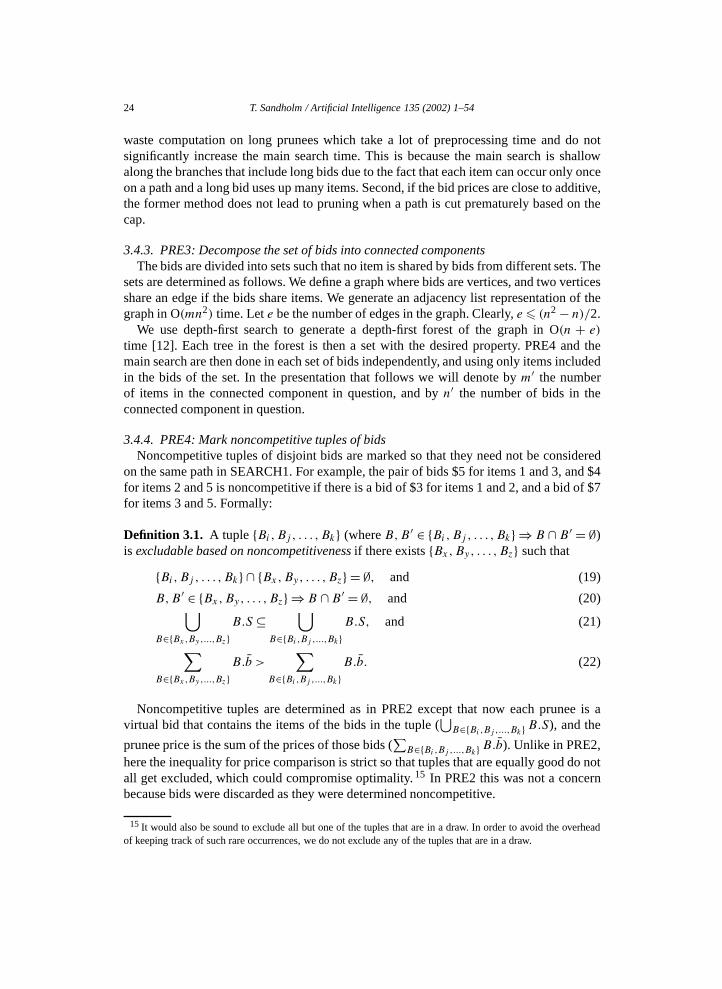
3.4.4. PRE4: Mark noncompetitive tuples of bidsNoncompetitive tuples of disjoint bids are marked so that they need not be considered
on the same path in SEARCH1. For example, the pair of bids $5 for items 1 and 3, and $4for items 2 and 5 is noncompetitive if there is a bid of $3 for items 1 and 2, and a bid of $7for items 3 and 5. Formally:
Definition 3.1. A tuple {Bi,Bj , . . . ,Bk} (where B,B ′ ∈ {Bi,Bj , . . . ,Bk} ⇒ B ∩B ′ = ∅)is excludable based on noncompetitiveness if there exists {Bx,By, . . . ,Bz} such that
{Bi,Bj , . . . ,Bk} ∩ {Bx,By, . . . ,Bz} = ∅, and (19)
B,B ′ ∈ {Bx,By, . . . ,Bz} ⇒ B ∩B ′ = ∅, and (20)⋃B∈{Bx,By,...,Bz}
B.S ⊆⋃
B∈{Bi ,Bj ,...,Bk}B.S, and (21)
∑B∈{Bx,By,...,Bz}
B.b >∑
B∈{Bi ,Bj ,...,Bk}B.b. (22)
Noncompetitive tuples are determined as in PRE2 except that now each prunee is avirtual bid that contains the items of the bids in the tuple (
⋃B∈{Bi ,Bj ,...,Bk}B.S), and the
prunee price is the sum of the prices of those bids (∑B∈{Bi ,Bj ,...,Bk}B.b). Unlike in PRE2,
here the inequality for price comparison is strict so that tuples that are equally good do notall get excluded, which could compromise optimality. 15 In PRE2 this was not a concernbecause bids were discarded as they were determined noncompetitive.
15 It would also be sound to exclude all but one of the tuples that are in a draw. In order to avoid the overheadof keeping track of such rare occurrences, we do not exclude any of the tuples that are in a draw.
T. Sandholm / Artificial Intelligence 135 (2002) 1–54 25
For computational speed, we only determine the noncompetitiveness of 2-tuples, thatis, pairs of bids. PRE4 is used as a partial preprocessor like PRE2, with caps Γ ′ or Φ ′instead of Γ or Φ . PRE4 runs in O(n′ cap+3(m′ − logn′)) time. This is because consideringall pairs of bids is O(n′2), the tree for each such pair is O(n′ cap), and finding a child inthe Bidtree is O(n′ · (m′ − logn′)). 16 Handling 3-tuples would increase the complexity toO(n′ cap+4(m′ − logn′)), etc. Handling large tuples also slows the main search because itneeds to ensure that noncompetitive tuples do not exist on the path.
As a bid is appended to the path in SEARCH1, it excludes from the rest of the paththose other bids that constitute a noncompetitive pair with it, and those bids that shareitems with it. Our algorithm determines this quickly as follows. For each bid, a list of bidsto exclude is determined in PRE4. In SEARCH1, an exclusion count is kept for each bid,starting at 0. As a bid is appended to the path, the exclusion counts of those bids that itexcludes are incremented. As a bid is backtracked from the path, those exclusion countsare decremented. Then, when searching for bids to append to the SEARCH1 path from theBidtree, only bids with exclusion count 0 are accepted. 17
3.5. Iterative deepening A∗ and heuristics
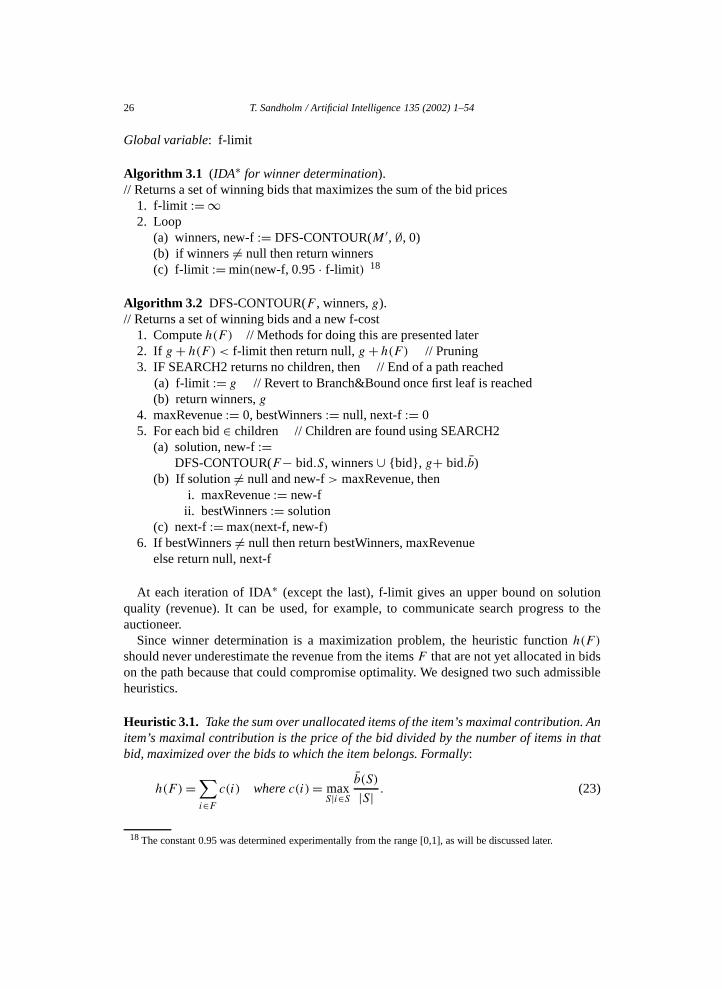
We sped up the main search by using an iterative deepening A∗ (IDA∗) searchstrategy [28] instead of depth-first search. The search tree, use of SEARCH2 in the Bidtreeto generate children of a SEARCH1 node, and the preprocessors stay the same. In practice,IDA∗ finds the provably optimal solution while searching a very small fraction of the entiresearch tree of SEARCH1 (Fig. 3). The following pseudocode shows how we applied theIDA∗ search strategy to the winner determination problem. The function h(F ), discussedin detail later, gives an upper bound on how much revenue the items F that are not yetallocated on the current search path can contribute. As defined earlier in this paper, g isthe sum of the prices of the bids that are on the current search path. At any search node, anupper bound on the total revenue that can be obtained by including that search node in thesolution is given by f = g+ h(F ).
Instead of using basic IDA∗ throughout the search, on the last IDA∗ iteration we keepincrementing the f-limit to equal the revenue of the best solution found so far in order toavoid futile search. In other words, once the first solution is found, our algorithm convertsto branch-and-bound with the same heuristic function, h. This modification is included inthe pseudocode below.
16 This analysis makes the innocuous assumption that m′ − logn′ � c for some constant c > 0 (recallProposition 3.5). Otherwise, the complexity of finding a child (actually, all children) is only O(n′).
17 PRE2 and PRE4 could be converted into anytime preprocessors without compromising optimality by startingwith a small cap, conducting the searches, increasing the cap, reconducting the searches, etc. Preprocessing wouldstop when it is complete (cap = n′), the user decides to stop it, or some other stopping criterion is met. PRE2 andPRE4 could also be converted into approximate preprocessors by allowing pruning when the sum of the pruners’prices exceeds a fixed fraction of the prunee’s price. This would allow more bids to be pruned which can makethe main search faster, but it can compromise optimality.
26 T. Sandholm / Artificial Intelligence 135 (2002) 1–54
Global variable: f-limit
Algorithm 3.1 (IDA∗ for winner determination).// Returns a set of winning bids that maximizes the sum of the bid prices
1. f-limit := ∞2. Loop
(a) winners, new-f := DFS-CONTOUR(M ′, ∅, 0)(b) if winners �= null then return winners(c) f-limit := min(new-f, 0.95 · f-limit) 18
Algorithm 3.2 DFS-CONTOUR(F , winners, g).// Returns a set of winning bids and a new f-cost
1. Compute h(F ) // Methods for doing this are presented later2. If g + h(F ) < f-limit then return null, g + h(F ) // Pruning3. IF SEARCH2 returns no children, then // End of a path reached
(a) f-limit := g // Revert to Branch&Bound once first leaf is reached(b) return winners, g
4. maxRevenue := 0, bestWinners := null, next-f := 05. For each bid ∈ children // Children are found using SEARCH2
(a) solution, new-f :=DFS-CONTOUR(F− bid.S, winners ∪ {bid}, g+ bid.b)
(b) If solution �= null and new-f > maxRevenue, theni. maxRevenue := new-f
ii. bestWinners := solution(c) next-f := max(next-f, new-f)
6. If bestWinners �= null then return bestWinners, maxRevenueelse return null, next-f
At each iteration of IDA∗ (except the last), f-limit gives an upper bound on solutionquality (revenue). It can be used, for example, to communicate search progress to theauctioneer.
Since winner determination is a maximization problem, the heuristic function h(F )should never underestimate the revenue from the items F that are not yet allocated in bidson the path because that could compromise optimality. We designed two such admissibleheuristics.
Heuristic 3.1. Take the sum over unallocated items of the item’s maximal contribution. Anitem’s maximal contribution is the price of the bid divided by the number of items in thatbid, maximized over the bids to which the item belongs. Formally:
h(F )=∑i∈Fc(i) where c(i)= max
S|i∈Sb(S)
|S| . (23)
18 The constant 0.95 was determined experimentally from the range [0,1], as will be discussed later.
T. Sandholm / Artificial Intelligence 135 (2002) 1–54 27
Proposition 3.6. h(F ) from Heuristic 3.1 gives an upper bound on how much revenue theunallocated items F can contribute.
Proof. For any set S ∈ F , if a bid for S is determined to be winning, then each of the itemsin S contributes b(S)/|S| toward the revenue. Every item can be in only one winning bid.Therefore, the revenue contribution of any one item i can be at most maxS|i∈S(b(S)/|S|).To get an upper bound on how much all the unallocated items F together can contribute,simply sum maxS|i∈S(b(S)/|S|) over all i ∈ F . ✷Heuristic 3.2. Identical to Heuristic 3.1 except that accuracy is increased by recomputingc(i) every time a bid is appended to the path since some other bids may now be excluded.A bid is excluded if some of its items are already used on the current path in SEARCH1,or if it constitutes a noncompetitive pair (as determined in PRE4) with some bid on thecurrent path in SEARCH1.
Proposition 3.7. h(F ) from Heuristic 3.2 gives an upper bound on how much revenue theunallocated items F can contribute.
Proof. Excluded bids cannot affect the revenue because they cannot be designated aswinning. Therefore, c(i) can be recomputed without the excluded bids, and the proof ofProposition 3.6 holds. ✷
We use Heuristic 3.2 with several methods for speeding it up. A tally of h is kept, andonly some of the c(i) values in h need to be updated when a bid is appended to the path.In PRE4 we precompute for each bid the list of items that must be updated: items includedin the bid and in bids that are on the bid’s exclude list. To make the update even faster, wekeep for each item a list of the bids in which it belongs. The c(i) value is computed bytraversing that list and choosing the highest b(S)/|S| among the bids that have exclusioncount 0. So, recomputing h takes O(m′n′) time, wherem′ is the number of items that needto be updated, and n′ is the (average or greatest) number of bids in which those itemsbelong. 19
3.6. Time complexity of the main search (SEARCH1)
The worst case time complexity of the main search is polynomial in bids and exponentialin items. This is desirable since the auctioneer can control the number of items forsale, but usually cannot control (and does not want to restrict) the number of bidsreceived.
19 PRE2 and PRE4 use depth-first search because due to the caps their execution time is negligible comparedto the main search time. Alternatively they could use IDA∗. Unlike in the main search, the c(i) values should becomputed using only combinations S that are subsets of the prunee. The f-limit in IDA∗ can be set to equal theprunee bid’s price (or a fraction thereof in the case of approximation), so IDA∗ will complete in one iteration.Finally, care needs to be taken that the heuristic and the tuple exclusion are handled correctly since they are basedon the results of the preprocessing itself.
28 T. Sandholm / Artificial Intelligence 135 (2002) 1–54
Specifically, by Proposition 3.3 the number of SEARCH1 nodes is O(m′ · (n′/m′)m′)
even without pruning. The time per each SEARCH1 node is O(n′m′) because each ofthe per node activities (child generation, h-function updating, etc.) is O(n′m′). IDA∗generates some nodes multiple times because all of the nodes generated in one iterationare regenerated in the next iteration. However, given that the new f-limit is loweredto the maximum f -value that was lower than the f-limit in the previous iteration (orto an even lower value), each iteration generates at least one more search node thanthe previous iteration. Therefore, if the number of nodes in a search tree is x , thenIDA∗ will generate at most x 1+x
2 search nodes. In practice it will generate significantlyfewer because the f-limit is decreased more across iterations, as was presented in thepseudocode and as will be discussed further in the section on experimental results.Nevertheless, even in the hypothetical worst case, the overall worst case complexityremains polynomial in bids because the regeneration of nodes in IDA∗ only increases thecomplexity polynomially.
The complexity in the number of bids is complexity in the number of bids actuallyreceived. This is in contrast to approaches such as the dynamic program which executesthe same steps independent of the bids that have been received.
4. Experimental setup
To determine the efficiency of the algorithm in practice, we ran experiments on a general-purpose uniprocessor workstation (450 MHz Sun Ultra 80 with 1 Gigabyte of RAM) inC++ with four different bid distributions:
• Random: For each bid, pick the number of items randomly from 1,2, . . . ,m.Randomly choose that many items without replacement. Pick the price randomly from[0,1].
• Weighted random: As above, but pick the price between 0 and the number of items inthe bid.
• Uniform: Draw the same number of randomly chosen items for each bid. Pick theprices from [0,1].
• Decay: Give the bid one random item. Then repeatedly add a new random item withprobability α until an item is not added or the bid includes all m items. Pick the pricebetween 0 and the number of items in the bid.
If the same bid was generated twice, the new version was deleted and regenerated. So, forexample, if the generator was asked to produce 500 bids, it produced 500 different bids.
We let all the bids have the same bidder. This conservative method causes PRE1 to pruneno bids. This is a good model of reality if the number of items is large and bidders placetheir bids on randomly chosen combinations, because then the chance that two agents bidon the same combination is small due to the number of combinations being large (2m− 1).However, in some cases PRE1 is very effective. In the extreme, it prunes all of the bidsexcept one if all bids are placed on the same combination by different bidders. When PRE1is effective, our algorithm will run faster than suggested by the conservative experimentsof this paper.

T. Sandholm / Artificial Intelligence 135 (2002) 1–54 29
5. Experimental results
We focus on IDA∗ (with branch-and-bound on the last iteration after the first leaf hasbeen reached) because it was two orders of magnitude faster than depth-first search. Welower the f-limit between iterations to 95% of the previous f-limit or to the highest valueof f that was lower than the f-limit in the previous IDA∗ iteration, whichever is smaller(as shown in the pseudocode of the previous section). Clearly, there is never any reason touse an f-limit that is higher than the highest value of f that was lower than the f-limit inthe previous IDA∗ iteration. The 95% criterion is used to decrease the f-limit even faster.Experimentally, this tended to be a good rate of decreasing the f-limit. If it is decreasedtoo fast, the overall number of search nodes increases because the last iteration will leadto a large number of search nodes in DFS-CONTOUR. If it is decreased too slowly, theoverall number of search nodes increases because new iterations repeat a large portion ofthe search from previous iterations.
For PRE2, the cap Φ = 8 gave a good compromise between preprocessing time andmain search time. For PRE4, Φ ′ = 5 led to a good compromise. These values are used inthe rest of the experiments. With these caps, the hard problem instances with short bids getpreprocessed completely, and PRE2 and PRE4 tend to take negligible time compared tothe main search because the trees under such short prunees are small. The caps only takeeffect in the easy cases with long bids. In the uniform distribution all bids are the samelength, so PRE2 does not prune any bids because no bid is a subset of another.
As expected, PRE3 saved significant time on the uniform and decay distributions bypartitioning the bids into connected components when the number of bids was smallcompared to the number of items, and the bids were short. On the other hand, in almostall of the experiments on the random and weighted random distributions, the bids fell intothe same connected component because the bids were long. In real world combinatorialauctions it is likely that the number of bids will significantly exceed the number of itemswhich would suggest that PRE3 does not help. However, in many practical settings the bidswill most likely be short, and the bidders’ interests often have special structure which leadsto some items being independent of each other, and PRE3 will automatically capitalize onthat.
The main search generated 35,000–40,000 nodes per second when the number of itemswas small (25) and the bids were short (3 items per bid). This rate decreased slightlywith the number of bids, but significantly with the number of items and bid size. With theweighted random distribution with 400 items and 2,000 bids, the search generated only12 nodes per second. However, the algorithm solved these cases easily because the searchpaths were short and the heuristic focused the search well. Long bids make the heuristic andexclusion checking slower but the search tree shallower which makes them easier for ouralgorithm than short bids overall. This observation is further supported by the results below.Each point in each graph represents an average over 15 problem instances. The executiontimes presented include all preprocessing times. For the problem sizes that we consider,previous optimal winner determination approaches (exhaustive enumeration and dynamicprogramming) cannot be used at all in practice because they would take prohibitively long,as was discussed earlier in this paper.
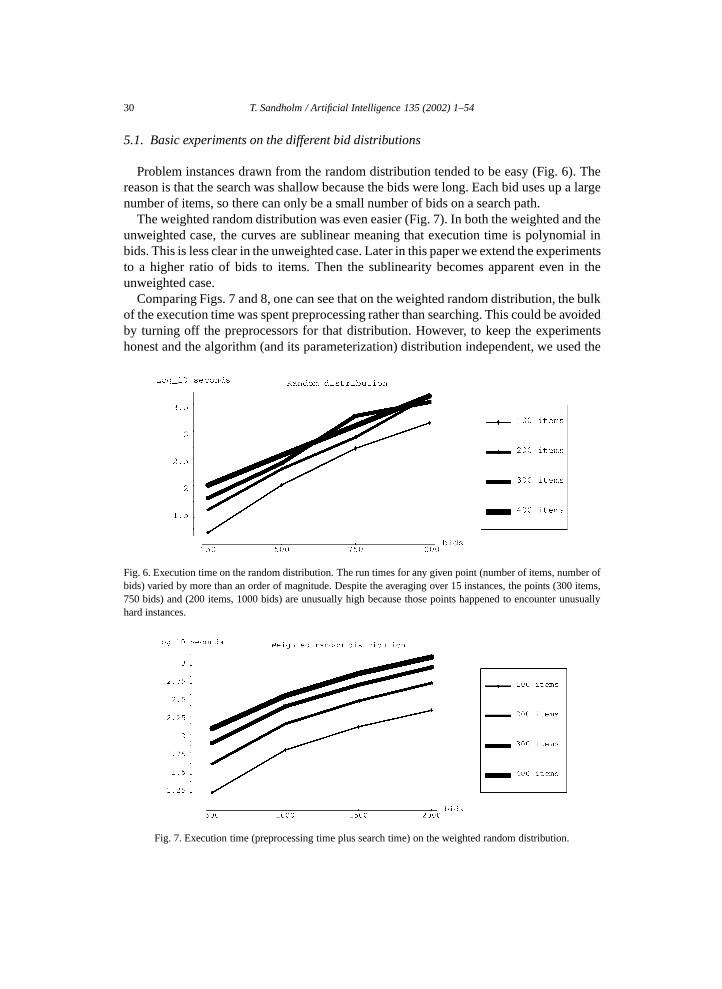
30 T. Sandholm / Artificial Intelligence 135 (2002) 1–54
5.1. Basic experiments on the different bid distributions
Problem instances drawn from the random distribution tended to be easy (Fig. 6). Thereason is that the search was shallow because the bids were long. Each bid uses up a largenumber of items, so there can only be a small number of bids on a search path.
The weighted random distribution was even easier (Fig. 7). In both the weighted and theunweighted case, the curves are sublinear meaning that execution time is polynomial inbids. This is less clear in the unweighted case. Later in this paper we extend the experimentsto a higher ratio of bids to items. Then the sublinearity becomes apparent even in theunweighted case.
Comparing Figs. 7 and 8, one can see that on the weighted random distribution, the bulkof the execution time was spent preprocessing rather than searching. This could be avoidedby turning off the preprocessors for that distribution. However, to keep the experimentshonest and the algorithm (and its parameterization) distribution independent, we used the
Fig. 6. Execution time on the random distribution. The run times for any given point (number of items, number ofbids) varied by more than an order of magnitude. Despite the averaging over 15 instances, the points (300 items,750 bids) and (200 items, 1000 bids) are unusually high because those points happened to encounter unusuallyhard instances.
Fig. 7. Execution time (preprocessing time plus search time) on the weighted random distribution.
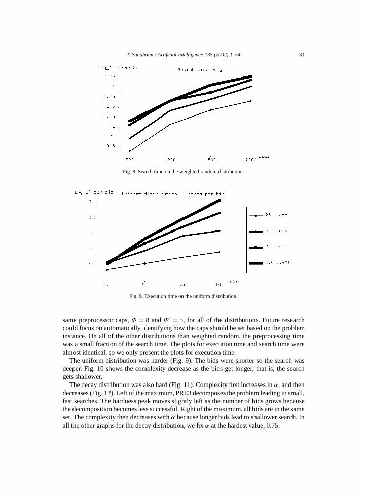
T. Sandholm / Artificial Intelligence 135 (2002) 1–54 31
Fig. 8. Search time on the weighted random distribution.
Fig. 9. Execution time on the uniform distribution.
same preprocessor caps, Φ = 8 and Φ ′ = 5, for all of the distributions. Future researchcould focus on automatically identifying how the caps should be set based on the probleminstance. On all of the other distributions than weighted random, the preprocessing timewas a small fraction of the search time. The plots for execution time and search time werealmost identical, so we only present the plots for execution time.
The uniform distribution was harder (Fig. 9). The bids were shorter so the search wasdeeper. Fig. 10 shows the complexity decrease as the bids get longer, that is, the searchgets shallower.
The decay distribution was also hard (Fig. 11). Complexity first increases in α, and thendecreases (Fig. 12). Left of the maximum, PRE3 decomposes the problem leading to small,fast searches. The hardness peak moves slightly left as the number of bids grows becausethe decomposition becomes less successful. Right of the maximum, all bids are in the sameset. The complexity then decreases with α because longer bids lead to shallower search. Inall the other graphs for the decay distribution, we fix α at the hardest value, 0.75.
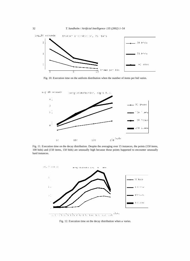
32 T. Sandholm / Artificial Intelligence 135 (2002) 1–54
Fig. 10. Execution time on the uniform distribution when the number of items per bid varies.
Fig. 11. Execution time on the decay distribution. Despite the averaging over 15 instances, the points (150 items,100 bids) and (150 items, 150 bids) are unusually high because those points happened to encounter unusuallyhard instances.
Fig. 12. Execution time on the decay distribution when α varies.

T. Sandholm / Artificial Intelligence 135 (2002) 1–54 33
5.2. Scaling up to larger numbers of bids
In practice, the auctioneer usually can control the number of items that are being sold in acombinatorial auction, but cannot control the number of bids that end up being submitted.Therefore, it is particularly important that the winner determination algorithm scales upwell to large numbers of bids. In this section we test how our algorithm scales to largenumbers of bids when we fix the number of items (m= 50).
Fig. 13 shows that on the random and weighted random distributions, the algorithmscales very well to large numbers of bids. The complexity is clearly polynomial in bids,and once the number of bids reaches a certain level, additional bids increase the complexityonly slightly.
The uniform and decay distributions were again harder (Fig. 14). However, even on thesedistribution, the curves are sublinear, meaning that execution time is polynomial in bids.
Fig. 13. Execution time on the random and weighted random distributions.
Fig. 14. Execution time on the uniform and decay distributions.
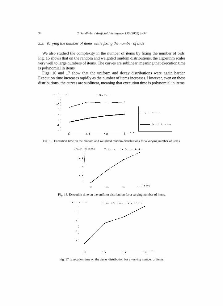
34 T. Sandholm / Artificial Intelligence 135 (2002) 1–54
5.3. Varying the number of items while fixing the number of bids
We also studied the complexity in the number of items by fixing the number of bids.Fig. 15 shows that on the random and weighted random distributions, the algorithm scalesvery well to large numbers of items. The curves are sublinear, meaning that execution timeis polynomial in items.
Figs. 16 and 17 show that the uniform and decay distributions were again harder.Execution time increases rapidly as the number of items increases. However, even on thesedistributions, the curves are sublinear, meaning that execution time is polynomial in items.
Fig. 15. Execution time on the random and weighted random distributions for a varying number of items.
Fig. 16. Execution time on the uniform distribution for a varying number of items.
Fig. 17. Execution time on the decay distribution for a varying number of items.

T. Sandholm / Artificial Intelligence 135 (2002) 1–54 35
5.4. Fixing the ratio of bids to items
From a practical perspective it seems reasonable that the number of bids grows as thenumber of items grows. Therefore, an additional experiment was called for where neitherthe number of items nor the number of bids was fixed. In this experiment we fixed the ratioof bids to items (n/m= 10).
Fig. 18 presents the execution times for the random and weighted random distributions.The curves are sublinear, which means that the execution time is polynomial in bids and initems.
Fig. 19 presents the execution times for the uniform and decay distributions. These wereagain significantly harder than the random and weighted random distributions.
Fig. 18. Execution time on the random and weighted random distributions.
Fig. 19. Execution time on the uniform and decay distributions.

36 T. Sandholm / Artificial Intelligence 135 (2002) 1–54
6. Incremental computations
In many auction settings it is important to provide results while the auction is still open.Motivated by this need, we designed incremental methods for computing results. Thefollowing subsections discuss incremental winner determination and incremental quotecomputation.
6.1. Incremental winner determination
In some auction settings it is important to be able to compute optimal solutions in theinterim after some bids have been received while others are still to be received. This allowsthe bidders to be told who the current winners would be if no further bids were to bereceived. This information can be naively produced by running the preprocessors and themain search from scratch every time a new bid arrives. However, the amount of redundantcomputation can be reduced by using the following observations.
1. Say that a new bid B = (B.S,B.b) has arrived since the winner determination waslast carried out. If PRE1 or PRE2 prune the new bid, that bid will not affect thesolution. It follows that the solution that was optimal before the new bid arrivedremains optimal, so PRE3, PRE4, and the main search need not be executed again.If the new bid is noncompetitive, it can be permanently discarded. Other bids thatarrive later on cannot make it competitive. Neither can this bid prune later bids thatwould not be pruned anyway.
2. If PRE1 and PRE2 do not prune the new bid B , then the winners can be determinedas follows. Let r∗old be the old optimal revenue without the new bid B . Now, conductthe winner determination with the items M −B.S, and with bids that do not includeany items in B.S. Call the new optimal revenue r∗M−B.S . If r∗M−B.S + B.S > r∗old ,then the optimal revenue is r∗M−B.S +B.S and the optimal solution includes the newbid B and the winning bids from this new winner determination. Otherwise, the oldrevenue r∗old and the corresponding bids are optimal.The winner determination with items M − B.S can be done in one IDA∗ iterationby setting the f-limit to r∗old − B.S. If IDA∗ returns no solution, then the old optimalsolution is best. On the other hand, if IDA∗ returns a solution, then that solution—together with bid B—is best.That single IDA∗ iteration can involve unnecessary search if the price of the newbid, B.b, is high relative to the prices of the old bids, because in such scenariosnew solutions that are better than the old solution can be found even while using ahigher f-limit, leading to more pruning in the search. One can reduce the numberof nodes generated in the last iteration by starting IDA∗ with a higher f-limit, andthen lowering it between iterations if a solution is not found. There is never a needto lower it below r∗old − B.S. One can start lowering the f-limit from some upperbound on r∗M−B.S . An upper bound, UB, UB � r∗M−B.S , is given by the revenue ofthe old optimum minus the highest revenue that could have been obtained from non-overlapping old bids whose items are contained in the new bid. Formally,
UB = r∗old − r∗old(B.S) (24)
T. Sandholm / Artificial Intelligence 135 (2002) 1–54 37
where
r∗old(B.S)= max{T |∀Ti,Tj∈T , Ti ,Tj⊆B.S and Ti∩Tj=∅}
∑T ∈T
b(T ), (25)
where b(T ) is computed using the old bids only.3. Incremental winner determination can be used even if several bids have arrived since
the most recent winner determination.Observation 1 from above can be extended to this setting. Both the old bids and newbids are used to prune new bids in PRE1 and PRE2. To determine whether the oldsolution is optimal, only new bids are pruned. If some of them do not get pruned, sothe solution needs to be recomputed, then old bids are also targets of pruning. An oldbid that was not pruned before might now be prunable in light of the new bids.Observation 2 from above can also be extended to this setting. If observation 1 fails,so PRE3, PRE4, and the main search do need to be executed, the old optimal revenue,r∗old , provides a lower bound on the new optimal revenue, r∗new. This lower boundcan be used as the initial f-limit in the main search so that IDA∗ completes in oneiteration. If IDA∗ returns a solution with that f-limit, then a new optimal solution hasbeen found that includes some of the new bids. Otherwise, the old optimal solutionremains best.That single IDA∗ iteration can involve unnecessary search if the prices of the newbids are high relative to the prices of the old bids, because in such a scenario a higherf-limit (leading to more pruning) can suffice for finding a new optimal solution thatis better than the old optimal solution. One can reduce the number of search nodes inthe last iteration by starting IDA∗ with a higher f-limit, and then lowering it betweeniterations if a solution is not found. There is never need to lower it below r∗old becauser∗new � r∗old. One can start lowering the f-limit from some upper bound on r∗new. Anupper bound, UBS , UBS � r∗new, is given by
UBS = max[r∗old, r
∗old + r∗(S)− r∗old(S)
], (26)
where
S =⋃
i∈ new bids
Bi.S, (27)
r∗(S) is the maximal revenue that can be obtained from the items S using the old andthe new bids, and r∗old(S) is the maximal revenue that can be obtained from the itemsS using the old bids only. These revenues can be determined using the preprocessingand search techniques of this paper, and if |S|< |M|, computing them is faster thancarrying out the overall winner determination.
6.2. Incremental quote computation
In some settings it is also important to be able to tell a prospective bidder how much shewould have to bid on any given combination, S, so that she would become the winner ofS given the other bids so far. For example, a bidder may post the following query: “How
38 T. Sandholm / Artificial Intelligence 135 (2002) 1–54
much would I have to bid to obtain the set of items S = {2,3,7} (assuming that no furtherbids will be submitted)?”. We developed several methods for computing such quotes:
1. Exact quote. Let r∗ be the revenue of the current optimal solution. Now, removethe items S and all bids that include items in S, and determine the winners againoptimally. Call the new revenue r∗reduced. Now, an exact quote on S is given byr∗ − r∗reduced.
2. Quote bounds. An upper bound on a quote (“If you bid $x, you will certainly get S(assuming that no further bids will be submitted)”) can be computed as an upperbound on (or exact value) r∗ minus a lower bound on (or exact value) r∗reduced.Similarly, a lower bound on a quote (“If you bid only $y, you will certainly notget S (assuming that no further bids will be submitted)”) can be computed as a lowerbound on (or exact value) r∗ minus an upper bound on (or exact value) r∗reduced.A lower bound can be computed using an approximation algorithm (such as thosediscussed earlier in this paper), or by running the anytime search algorithm of thispaper for some amount of time. An earlier solution that was obtained without some ofthe newest bids can also be used as a lower bound. This allows winner determinationto run only occasionally while still supporting approximate quotes in the meantime.One can also compute several of these lower bounds and provide the highestone.An upper bound can be computed using a linear programming relaxation of theproblem (discussed further in Section 8), or by using the h-function value directlyas the upper bound. Alternatively, the f-limit in IDA∗ can be used as an upperbound. Since the f-limit does not provide an upper bound on the last IDA∗ iteration,and one does not know in advance whether the current iteration will be the last,one can use the highest value of f that was lower than the f-limit in the previousiteration. As yet another alternative, one can use the incrementally computed upperbound, UBS , from the previous subsection. This allows winner determination torun only occasionally while still supporting approximate quotes in the meantime.One can also compute several of these upper bounds and provide the lowestone.
3. Binary search for a quote and quote bounds. A hypothetical bid is placed oncombination S. Binary search is carried out on the price of that new bid, runningthe preprocessors and the main search algorithm for each price that the binary searchgenerates for the new bid. Observations 1 and 2 from the previous subsection canbe directly used to speed up the execution within each such price point. If theprice is very low, the preprocessors can quickly determine that the hypotheticalbid is not competitive. This provides a lower bound on the quote and let’s thebinary search proceed further. If the price is very high, the search will quickly findsolutions that include the new bid and give revenue that exceeds the revenue that wasobtainable without that bid. When this occurs, the search can be interrupted becausean upper bound on the quote has been established, and the binary search can proceedfurther.
T. Sandholm / Artificial Intelligence 135 (2002) 1–54 39
6.2.1. Properties of quotesQuotes (even exact quotes) in combinatorial auctions have some interesting properties.
First, the quote on a combination is not necessarily the sum of the quotes on individualitems:
Proposition 6.1. Quotes in a combinatorial auction are not always additive.
Proof. Consider an auction of two items: 1 and 2. Say that three bids have been submitted:$4 for item 1, $1 for item 2, and $6 for the combination {1,2}. Now, the quote for item 1is $5, the quote for item 2 is $2, and the quote for the combination {1,2} is $6. But $5 +$2 �= $6. ✷
This means that providing quotes on individual items does not provide enoughinformation for a bidder who prefers combinations.
In usual single-item auctions, the quote can increase (or stay the same) as a new bidarrives. New bids cannot reduce the quote. However, this monotonicity ceases to hold incombinatorial auctions:
Proposition 6.2. As a bid is submitted on some combination (or individual item) in acombinatorial auction, the quotes on other combinations (and individual items) mightincrease or decrease.
Proof. Consider the example from the proof of Proposition 6.1. Say that a new bid of $7 issubmitted on combination {1,2}. Now, the quote on item 1 increases to $6, and the quoteon item 2 increases to $3.
If, instead, a bid of $4.5 is submitted for item 1, then the quote on item 2 decreases to$1.5. ✷
Finally, if a bid is currently a winner, then the quote on the set of items of that bid issimply the price of that bid.
7. Other applications for the algorithms
The algorithms for winner determination can be directly used to solve weighted setpacking, weighted independent set, and weighted maximum clique because they are infact analogous problems. In addition they can be used for coalition structure generation incharacteristic function games. The characteristic function assigns a value to each potentialcoalition of agents. The objective is to partition the agents exhaustively into disjoint coali-tions so as to maximize the sum of the values of those coalitions. The agents correspondto items, coalitions to combinations, and coalition values to bid prices. This problem isanalogous to the winner determination problem if the coalitions have nonnegative values.This can usually be achieved by normalizing if it does not hold up front. However, coalitionstructure generation differs from winner determination in two major ways.
First, the values of most coalitions are usually nonzero so the space of “bids” is denselypopulated. That reduces the usefulness of algorithms that capitalize on the sparseness ofbids. This speaks in favor of using the dynamic program. However, that will not scale uppast small numbers of agents either.
40 T. Sandholm / Artificial Intelligence 135 (2002) 1–54
Second, in coalition structure generation the values of coalitions might not be known toany party, and only values of complete coalition structures might be known, or they becomeknown during a search process. Sandholm et al. [49] recently proved inapproximabilityresults and devised an anytime approximation algorithm with worst case guarantees forthis case which is harder than the case where the values of coalitions are observed.
8. Related tree search algorithms
A significant amount of work in the field of operations research has focused on problemsthat are analogous to the combinatorial auction winner determination problem, particularlyweighted set packing and weighted independent set. The approximation approaches werediscussed in detail earlier in this paper. In addition, considerable research has been doneon exact algorithms for these problems. These algorithms typically use a branch-and-bound search strategy where an h-function value (that is, an upper bound on how muchrevenue the yet unallocated items can contribute) is computed from the linear programmingproblem that is obtained by taking the winner determination problem (with the items andbids that are still usable given the bids that are already on the search path) and changing theconstraints xS ∈ {0,1} to xS � 1. This linear program at each search node can be solvedin polynomial time in the size of the input (which itself is *(nm)) using interior pointmethods, or fast on average using the simplex method [11,60]. The upper bound that thelinear programming relaxation provides can be tightened (lowered) by introducing cuts.These are additional constraints that do not affect the solution of the integer program,but which constrain the linear programming polytope. Major research questions in thesealgorithms include inventing new sound cuts, constructing fast algorithms for constructingcuts, as well as experimenting on the tradeoff between the time spent on generating cutsand the time saved due to the reduction in search tree size that stems from the tighterupper bounds. This is a vast literature (see, for example, [16,33,39]). There are severalmodern books on this approach [11,60], and good overviews of applying this approach tocombinatorial auctions have been written very recently [13,37]. Generally this approachleads to a smaller number of search nodes than our approach (due to tighter upper bounds),but spends more time per search node. Which is faster overall depends on the probleminstance distribution. Instead of viewing these two approaches as mutually exclusive,they can be viewed as complementary. A hybrid algorithm could use techniques bothfrom our approach (the preprocessors, fast child generation methods, the combination ofIDA∗ and branch-and-bound that we use, the h-function that is fast to compute, etc.) andthe traditional integer programming approach (using a linear programming relaxation toprovide upper bounds, introducing cuts, etc.). For example, a hybrid algorithm could usethe slow but relatively accurate linear programming relaxation only occasionally, whileusing our fast h-function to provide upper bounds for most search nodes. Also, it is alwayssound to compute both types of upper bounds, and to use the lowest of them.
After this paper was circulated as a technical report, and while it was under review forArtificial Intelligence, a very similar algorithm, called CASS, was published by Fujishimaet al. [15]. In fact, they present two algorithms, VSA and CASS. Here we focus on CASSbecause VSA does not generally find the optimal solution. Despite significant similarities,CASS differs from our algorithm in certain ways. CASS uses a branch-and-bound search

T. Sandholm / Artificial Intelligence 135 (2002) 1–54 41
strategy while we use IDA∗ combined with branch-and-bound. Neither search strategyalways dominates the other. IDA∗ can lead to fewer search nodes because the f-limit allowspruning of parts of the search space that branch-and-bound would search. On the otherhand, branch-and-bound can lead to fewer search nodes because IDA∗ searches the nodesthat are close to the root multiple times.
CASS uses a basic O(mn) child generation technique while we developed a moreelaborate method for O(n · (m− logn)) child generation. CASS uses binning to improvethe average case speed of child generation. Specifically, CASS keeps m lists of bids. Ineach list are all those bids that include item i , i ∈ {1, . . . ,m}. Then, to find the children ofa node, the algorithm only needs to loop through one of these list: the one where i = i∗(recall that i∗ is the smallest index among the items that are not on the path yet). Thisbinning technique has also been used by Garfinkel and Nemhauser [16].
CASS uses a rough approximation of our h-function, but one which supports computingthe h-function values in advance rather than during search. CASS also uses caching whilewe do not. Caching could be directly incorporated into our algorithm as well.
CASS relabels the items before the search so that promising bids are tried early inthe search. This relabeling could be directly incorporated into our algorithm as well.Experimentally it proved to be very effective in CASS. CASS also uses child orderingheuristics (which determine the order in which children of a node are considered).Incorporating child ordering heuristics into our algorithm is not as straightforward becauseour incremental child generation using the Bidtree imposes a particular order of thechildren as was discussed in Section 3.2.1. However, child ordering heuristics could beincorporated into our algorithm by generating all of the children of a node in a batch usingthe Bidtree, and then ordering the children before the search proceeds to any of them.Finally, CASS does not use as sophisticated preprocessing as we do. Our preprocessorscould be used in conjunction with CASS as well.
9. Substitutability, XOR-bids, and OR-of-XORs bidding
The methods for winner determination that were reviewed early in this paper, and mostother work on combinatorial auctions (see for example [14,42]), are based on a settingwhere each bidder can bid on combinations of items, any number of a bidder’s bids can beaccepted. This works well when bids are superadditive: b(S∪S′)� b(S)+ b(S′). However,when some of the bids are not superadditive, this can lead to problems. For example,what happens if agent 1 bids b1({1})= $5, b1({2}) = $4, and b1({1,2})= $7, and thereare no other bidders? The auctioneer could allocate items 1 and 2 to agent 1 separately,and that agent’s bid for the combination would value at $5 + $4 = $9 instead of $7. So,the current techniques focus on capturing synergies (complementarities) among items. Inpractice, local substitutability (subadditivity of the bid prices) can occur as well. As asimple example, when bidding for a landing slot for an airplane, the bidder is willing totake any one of a host of slots, but does not want more than one.
We address this issue in our Internet auction house prototype which is part ofour electronic commerce server called eMediator (see http://www.cs.cmu.edu/˜amem/eMediator). We developed a bidding language where the bidders can submit XOR-bids,
42 T. Sandholm / Artificial Intelligence 135 (2002) 1–54
that is, bids on combinations such that only one of the bids can get accepted. This allowsthe bidders to express general preferences with both complementarity and substitutability(see also [47] and [40]). In other words, the bidder can express any value functionv : 2m → R. 20 For example, a bidder in a 4-item auction may submit the following inputto the auctioneer:
({1},$4) XOR ({2},$4) XOR ({3},$2) XOR ({4},$2) XOR
({1,2},$8) XOR ({1,3},$6) XOR ({1,4},$6) XOR
({2,3},$6) XOR ({2,4},$6) XOR ({3,4},$3) XOR
({1,2,3},$10) XOR ({1,2,4},$10) XOR ({1,3,4},$7) XOR
({2,3,4},$7) XOR ({1,2,3,4},$11).
Such fully expressive bidding languages have several advantages. First, each bidder canexpress her preferences rather than having to approximate them with an utterance in someless expressive bidding language. This extra expressiveness generally also increases theeconomic efficiency of the allocation because the winner determination algorithm takesas input the fully expressive bids rather than approximations. Second, a fully expressivebidding languages enables the auctioneer to extract truthful valuation revelations as thebids. With a fully expressive bidding language, bidding truthfully can be made incentivecompatible (a dominant strategy) by using the Vickrey–Clarke–Groves mechanism [7,17,58]. This means that each bidder is motivated to bid truthfully regardless of how othersbid. This renders counterspeculation unnecessary. The Vickrey–Clarke–Groves mechanismcan be applied to the combinatorial auction setting as follows, assuming that a fullyexpressive bidding language is being used. Winning bids are determined so as to maximizethe auctioneer’s revenue under the constraint that each item can be allocated to at mostone bid. The amount that an agent needs to pay is the sum of the others’ winning bidshad the agent not submitted any bids, minus the sum of the others’ winning bids in theactual optimal allocation. Therefore, the winner determination problem has to be solvedonce overall, and once per winning agent without any of that agent’s bids. This makesfast winner determination even more crucial. Note that, for example, just removing onewinning bid at a time would not constitute an incentive compatible mechanism. Incentivecompatibility can also be lost if either winner determination or price determination is doneapproximately.
While XOR-bids are fully expressive, representing one’s preferences in that languageoften leads to large numbers of bids that are all combined with XOR. To maintainfull expressiveness, but at the same time to make the representation more concise, wepropose another bidding language which we call OR-of-XORs. This is also supportedin eMediator. In this language, a set of bids can be combined with XOR, forming andXOR-disjunct. These XOR-disjuncts can then be combined with non-exclusive ORs torepresent independence. For example, a bidder who wants to submit the same offer asin the example above, can do so by submitting the following more concise input to theauctioneer:
20 By default, the bid for the empty set of items is 0.
T. Sandholm / Artificial Intelligence 135 (2002) 1–54 43
[({1},$4)]OR
[({2},$4)]OR
[({3},$2) XOR ({4},$2) XOR ({3,4},$3)].Note that the simple XOR-bidding language is a special case of the OR-of-XORs language.Therefore, the shortest way to represent any particular value function in the OR-of-XORslanguage is never longer than in the simple XOR-bidding language.
Since the traditional winner determination problem with no XORs is a special caseof winner determination in the OR-of-XORs bidding language, the NP-completenessand inapproximability results apply to winner determination in the OR-of-XORs biddinglanguage as well. 21
9.1. Winner determination with XORs
Our winner determination algorithm can be easily adapted to handle XOR-constraintsbetween bids, be it in the simple XOR-bidding language, in the OR-of-XORs language, orin a language where the bidder can place XOR-constraints arbitrarily between bids. If twobids are in the same XOR-disjunct, and one of these bids is appended to the search pathin SEARCH1, then the other one should be excluded from being appended to that searchpath. As discussed earlier in this paper, exclusion also occurs if two bids share items, orif two bids constitute a noncompetitive pair (as determined in PRE4). Therefore, as wasdiscussed, an exclusion mechanism is already part of the algorithm. For each bid, a list ofbids to exclude is kept. Then, when a bid is appended to the search path in SEARCH1, theexclusion counts of all the bids that this bid excludes are incremented (and decrementedonce this bid is backtracked from the search path). At any point of the search, only bidswith exclusion count 0 are considered for appending to the search path.
Now, handling XORs in the algorithm is easy. Whenever two bids are in the same XOR-disjunct, they are simply added to each others’ exclusion lists, and the algorithm will handleXORs correctly. XOR-constraints reduce the size of the search space, so the search can befaster with such constraints than without.
9.2. Preprocessing with XORs
The preprocessors do not work directly with XOR-constraints. In this section we uncoverwhat the issues are, and design modifications to the preprocessors so that they correctlyhandle XOR-constraints.
21 After this paper was circulated as a technical report, and while it was under review for Artificial Intelligence,another fully expressive input method was proposed [15]. In that approach, whenever bids are to be mutuallyexclusive, a dummy item is created that is included in those bids. Therefore, the bids cannot ever occur togetherin a solution because they share an item.
44 T. Sandholm / Artificial Intelligence 135 (2002) 1–54
9.2.1. First preprocessor (PRE1)Consider a 2-item auction where bidder one has submitted
[({1},$4) XOR ({2},$3)]and bidder two has submitted
[({1},$2)].Now, the naive application of PRE1 would use the bid ({1},$4) to permanently remove thebid ({1},$2), and the maximal revenue would then be $4. However, by accepting the bids({2},$3) and ({1},$2), the auctioneer can achieve a revenue of $5. In other words, PRE1discarded a bid when it should not have.
PRE1 can be easily modified to correctly handle XOR-constraints between bids. This isachieved by having PRE1 discard bids less aggressively. First, a bid can be used to pruneanother bid (for the same set of items) if the bids are in the same XOR-disjunct. 22 Second,a bid can be used to prune a bid (for the same set of items) from another XOR-disjunct ifthe former bid is alone in its XOR-disjunct.
9.2.2. Second preprocessor (PRE2)Consider a 4-item auction where bidder one has submitted
[({1,2,3,4},$10)]and bidder two has submitted
[({1,3},$4) XOR ({2,4},$7)].Now, the naive application of PRE2 would use the bids ({1,3},$4) and ({2,4},$7) to prunethe bid ({1,2,3,4},$10). However, after that pruning the maximal revenue will be only $7while it should be $10. In other words, PRE2 discarded a bid when it should not have.
PRE2 can be easily modified to correctly handle XOR-constraints between bids. This isachieved by having PRE2 discard bids less aggressively. First, when pruning a bid withinone XOR-disjunct, only allow one bid to prune another (when the former bid’s item setis a subset of the latter bid’s, and the former bid’s price is higher or equal to the latterbid’s price) rather than allowing a set of bids to prune a bid as PRE2 does without XOR-constraints. This is because the bids in the set cannot actually occur together because theyare combined with XOR. Second, bids can be used to prune a bid from a different XOR-disjunct, given that each of the former bids is alone in its XOR-disjunct.
9.2.3. Third preprocessor (PRE3)Consider a 2-item auction where a bidder has submitted
[({1},$4) XOR ({2},$3)].Now, the naive application of PRE3 would decompose the problem into two connectedcomponents, each with one bid. Then, the winner determination would run independently
22 This is likely to be of limited value in practice since there seems to be no reason for having multiple bids forthe same set of items in one XOR-disjunct.
T. Sandholm / Artificial Intelligence 135 (2002) 1–54 45
on each connected component with a total revenue of $7, while the actual maximal revenueis only $4. In other words, PRE3 decomposed the problem when it should not have.
PRE3 can be easily modified to correctly handle XOR-constraints between bids. Thisis achieved by having PRE3 decompose the problem less aggressively. Specifically, in thegraph that PRE3 constructs for the purpose of identifying connected components, an extraedge is added between every pair of bids that are in the same XOR-disjunct. Then, asbefore, the connected components are identified in the graph, and PRE4 as well as themain search are carried out on each connected component separately.
9.2.4. Fourth preprocessor (PRE4)Consider an auction where bidder one has submitted
[({1,3},$5)],bidder two has submitted
[({2,5},$4)],and bidder three has submitted
[({1,2},$3) XOR ({3,5},$7)].Now, the naive application of PRE4 would use the bids ({1,2},$3) and ({3,5},$7) to markthe pair of bids ({1,3},$5) and ({2,5},$4) noncompetitive together. This would lead to amaximal revenue of only $7, while the actual maximal revenue is $9.
PRE4 can be easily modified to correctly handle XOR-constraints between bids. Thisis achieved by having PRE4 mark tuples of bids noncompetitive less aggressively. First, ifbids are in the same XOR-disjunct, they never need to be marked noncompetitive togetherbecause the XOR-constraint already ensures that they will never be on the same searchpath in SEARCH1. Second, bids can be used to mark bids from different XOR-disjunctsnoncompetitive together, given that each of the former bids is alone in its XOR-disjunct.
9.3. Incremental winner determination and quotes with XORs
The incremental techniques for determining winners and computing quotes, discussedin Section 6, can easily be used even when XOR-constraints between bids are allowed.The only modification to the incremental techniques is that the main search and thepreprocessors have to be adjusted as discussed in the previous subsections.
10. Conclusions and future research
Combinatorial auctions, that is, auctions where bidders can bid on combinations ofitems, tend to lead to more efficient allocations than traditional auction mechanisms inmulti-item auctions where the agents’ valuations of the items are not additive. This is be-cause the users can express complementarities in their bids, and the winner determinationalgorithm will take these into account. This paper tackled winner determination in com-binatorial auctions where each bidder can bid on unrestricted combinations of items. In
46 T. Sandholm / Artificial Intelligence 135 (2002) 1–54
such settings, determining the winners so as to maximize the auctioneer’s revenue is NP-complete.
The space of partitions of items was first explicated, and closed form asymptotic upperand lower bounds on the number of exhaustive partitions were derived. That number isso large that enumeration will only work with a very small number of items. Dynamicprogramming avoids some of the redundancy, but it does not scale beyond auctions witha small number of items because it generates the entire search space independent of whatbids have actually been received. We showed under what conditions the running time scalespolynomially.
The approach of compromising optimality to achieve polynomial-time winner deter-mination is futile if one is interested in worst case approximation guarantees: using therecently proven inapproximability of maximum clique, we proved that the winner deter-mination problem is inapproximable. If the combinations are restricted, somewhat betterguarantees can be established by known approximation algorithms for the weighted inde-pendent set problem and the weighted set packing problem, but the guarantees remain soweak that they are unlikely to be useful in the domain of auctions in practice. The mainhope for practical approximations for special cases lies in new forms of special structure—especially on bid prices.
By imposing severe restrictions on the allowable combinations, optimal winnerdetermination can be guaranteed in polynomial time. However, these restrictions introducesome of the same economic inefficiencies that are present in non-combinatorial auctions.
To tackle the limitations of the existing approaches to winner determination, wedeveloped a search algorithm for optimal winner determination. Via experiments on severaldifferent bid distributions that we introduced, we showed that our algorithm significantlyenlarges the envelope of inputs for which combinatorial auctions with optimal winnerdetermination are computationally feasible. The highly optimized algorithm achieves thismainly by capitalizing on the fact that the space of bids is often sparsely populated inpractice. Unlike dynamic programming, it generates only the populated parts of the searchspace. The algorithmic methods to implement this include provably sufficient selectivegeneration of children in the search tree, a secondary search to find children quickly, andheuristics that are admissible and optimized for speed. The algorithm also preprocessesthe search space by keeping only the highest bid for each combination, by removingbids that are provably noncompetitive (this is determined via search), by decomposingthe problem into independent parts, and by marking noncompetitive tuples of bids (this isagain determined via search).
The IDA∗ search algorithm, used in our main search, can easily be distributed acrossmultiple computers for additional speed [41]. The burden of search could also be imposedon the bidders by giving each bidder a portion of the search space to explore. Thisintroduces two risks. First, a bidder may only search her portion partially so as to savecomputational effort. Such free-riding can be desirable to her since the other bidders arelikely to find good solutions anyway—assuming that they themselves do not free-ride.Second, a bidder may report a suboptimal solution if that solution leads to a higher payofffor her. To prevent these problems, the auctioneer can randomly select one or more biddersafter they have reported the best solutions that they found, and re-search their portions. If,in some portion, the auctioneer finds a better solution than the reported one, the bidder gets
T. Sandholm / Artificial Intelligence 135 (2002) 1–54 47
caught of fraudulent searching, and a penalty can be imposed. If the penalty is high enoughcompared to the cost of computation and compared to the maximal gain from reportinginsincerely, and if the probability of getting checked upon is sufficiently high, each bidderis motivated to search her portion truthfully.
The algorithms for winner determination can be directly used to solve weighted setpacking, weighted independent set, and weighted maximum clique because they are in factthe analogous problem. Coalition structure generation in characteristic function games isalso a very similar problem, but it often has differing features as we discussed.
We presented techniques for incremental winner determination and quote computation.We also showed that quotes are nonadditive, and that a new bid may increase or decreasethe quotes on other combinations.
We showed that basic combinatorial auctions only allow bidders to express complemen-tarity of items. We then proposed a bidding language called XOR-bids. It is fully expressiveso the bidders can express both complementarity and substitutability. We discussed howthis bidding language enables the use of the Vickrey–Clarke–Groves mechanism to con-struct a combinatorial auction where every bidder’s dominant strategy is to bid truthfullyrather than strategically. We then introduced another fully expressive bidding languagecalled OR-of-XORs. It has all the advantages of XOR-bids, and is more concise. Finally,we extended our search algorithm and preprocessors to handle both of these languages andlanguages where XOR-constraints can be arbitrarily inserted between bids.
Our search algorithm can easily be extended to settings where the auctioneer cannotkeep items. This is accomplished by not using dummy bids and by considering a solutionfeasible (at any search node) if and only if all of the items are allocated to bidders. In suchsettings, some bids with negative (and zero) prices may have to be accepted.
In our current work we are developing even faster winner determination algorithmsfor combinatorial auctions [53,56], and algorithms for clearing combinatorial reverseauctions and exchanges [47,53,57]. We are also studying the impact of side constraintsand non-price attributes on the complexity of clearing combinatorial markets [55]. In thedirection of more restricted market designs, we are studying the complexity of clearingmarkets where the goods that are for sale are identical, and the bidders may use differentbidding languages such as supply/demand curves [54]. Finally, we are studying selectivebid elicitation in combinatorial auctions [9,10] and are designing optimal bidding agentsthat may not know their own valuations for bundles ex ante, but rather have to computethem [29,30,44,48].
Acknowledgements
I thank Kate Larson who significantly contributed to the proof of Proposition 2.1. I alsothank two anonymous reviewers for their helpful comments.
Appendix A. Proof of Proposition 2.1
Proof. We first prove that the number of exhaustive partitions is O(mm). Let there be mitems in the auction. Let there be a set of locations where combinations of items can form,
48 T. Sandholm / Artificial Intelligence 135 (2002) 1–54
at most one combination per location. Let the number of locations be m. Let any stateof all m locations together be a candidate for an exhaustive partition. This allows for anyexhaustive partition to form since an exhaustive partition can have at mostm combinations.Now, say that the items get placed in locations one item at a time. Each item could beplaced in m different locations, and there are m items to place. Therefore, the number ofcandidates is mm. Thus, the number of exhaustive partitions is O(mm). 23
What remains to be proven is that the number of exhaustive partitions is ω(mm/2). Weuse the following lemma in the proof.
Lemma A.1. Let a and b be positive integers. Then⌈a
b
⌉! �
(a
b
)a/bfora
b� 2.
Proof.
� ab�!
( ab)a/b
�ab
+ 1ab
·abab
·ab
− 1ab
· · · 2ab
�ab
+ 1ab
·ab
− 1ab
=(
1 + b
a
)(1 − b
a
)
= 1 −(b
a
)2
� 1.
Therefore � ab�! � ( a
b)a/b. ✷
One way to count the number of exhaustive partitions is to use Bell numbers. TheBell number βm is equal to the number of exhaustive partitions that can be generatedwith m items. There are several ways of calculating Bell numbers, including Dobinski’sformula [8]:
βm = 1
e
∞∑i=0
im
i! .
To show that the number of exhaustive partitions is ω(mm/2) it suffices to show that
limm→∞
βm
mm/2= ∞.
Since each term in the series of Dobinski’s formula is positive, it suffices to take one term,im/i! and show that
limm→∞
im/i!mm/2
= ∞.
23 The number of candidates, mm, overestimates the number of exhaustive partitions. Some exhaustive partitionsare counted multiple times because for any given combination in the exhaustive partition, the exhaustive partitionis counted once for each location where the combination can form (although it should be counted only once).
T. Sandholm / Artificial Intelligence 135 (2002) 1–54 49
Set i = �m/b� for some constant b, where b > 2. Then the expression we are interested inis
(�mb�)m
(�mb�)!mm/2 �
(mb)m
(�mb�)!mm/2 �
(mb)m
(mb)m/bmm/2
= mm(b−2)/2b
bm(b−1)/b.
We now calculate
limm→∞
mm(b−2)/2b
bm(b−1)/b.
Since the natural logarithm and exponential functions are continuous, we can calculate thelimit as follows. Let
φ(m) = lnmm(b−2)/2b
bm(b−1)/b
= m(b− 2)
2blnm− m(b− 1)
blnb
= m
b
[b− 2
2lnm− (b− 1) lnb
].
Then
limm→∞
mm(b−2)/2b
bm(b−1)/b= limm→∞ eφ(m)
= limm→∞ em/be((b−2)/2) lnm−(b−1) lnb
= limm→∞ em/b lim
m→∞ e((b−2)/2) lnm−(b−1) lnb
= ∞ · ∞= ∞.
Thus, we have shown that βm ∈ ω(mm/2). ✷
Appendix B. Proof of Proposition 3.5
Proof. Throughout the proof, when we use the term “tree”, we mean a tree that has nleaves, all at depth m+ 1, and has nodes with 1 or 2 children each. Because the numberof leaves in the tree is n, the number of binary nodes (nodes with two children) has to ben− 1. The rest of the nodes have to be unary (nodes with one child each). The claim isthat a worst case (case with the largest number of edges given n) can be constructed byhaving all of the binary nodes as close to the root as possible. Specifically, depths 1 to�logn� of the tree consist of binary nodes only, and the remaining binary nodes, if any, areat depth �logn� + 1. We will call any such tree a wide-early-tree. Fig. B.1 (left) illustratesa wide-early-tree where n is a power of 2 so there are no binary nodes at depth �logn�+ 1.For any given n, all wide-early-trees (which differ only based on how the binary nodes aredistributed at depth �logn�+ 1) have the same number of edges. Assume, to contradict theclaim, that there is some tree T that has n leaves, all at depthm+1, and T has n−1 binary
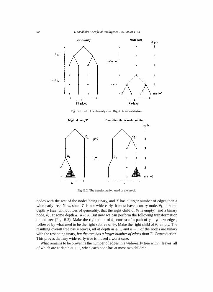
50 T. Sandholm / Artificial Intelligence 135 (2002) 1–54
Fig. B.1. Left: A wide-early-tree. Right: A wide-late-tree.
Fig. B.2. The transformation used in the proof.
nodes with the rest of the nodes being unary, and T has a larger number of edges than awide-early-tree. Now, since T is not wide-early, it must have a unary node, θ1, at somedepth p (say, without loss of generality, that the right child of θ1 is empty), and a binarynode, θ2, at some depth q , p < q . But now we can perform the following transformationon the tree (Fig. B.2). Make the right child of θ1 consist of a path of q − p new edges,followed by what used to be the right subtree of θ2. Make the right child of θ2 empty. Theresulting overall tree has n leaves, all at depth m+ 1, and n− 1 of the nodes are binarywith the rest being unary, but the tree has a larger number of edges than T . Contradiction.This proves that any wide-early-tree is indeed a worst case.
What remains to be proven is the number of edges in a wide-early tree with n leaves, allof which are at depth m+ 1, when each node has at most two children.
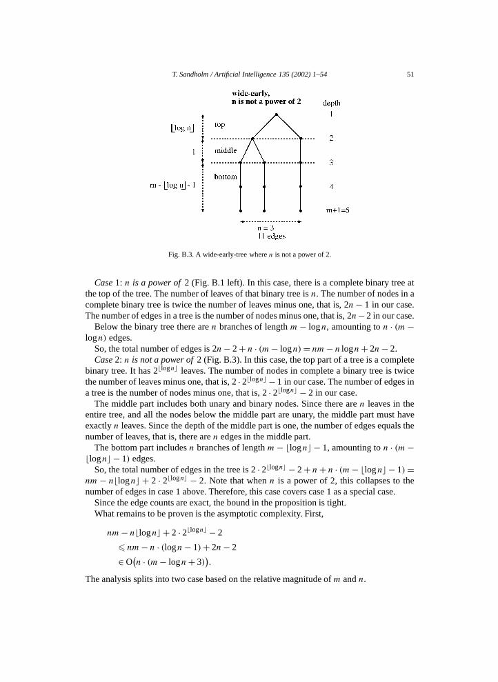
T. Sandholm / Artificial Intelligence 135 (2002) 1–54 51
Fig. B.3. A wide-early-tree where n is not a power of 2.
Case 1: n is a power of 2 (Fig. B.1 left). In this case, there is a complete binary tree atthe top of the tree. The number of leaves of that binary tree is n. The number of nodes in acomplete binary tree is twice the number of leaves minus one, that is, 2n− 1 in our case.The number of edges in a tree is the number of nodes minus one, that is, 2n− 2 in our case.
Below the binary tree there are n branches of length m− logn, amounting to n · (m−logn) edges.
So, the total number of edges is 2n− 2 + n · (m− logn)= nm− n logn+ 2n− 2.Case 2: n is not a power of 2 (Fig. B.3). In this case, the top part of a tree is a complete
binary tree. It has 2�logn� leaves. The number of nodes in complete a binary tree is twicethe number of leaves minus one, that is, 2 · 2�logn� − 1 in our case. The number of edges ina tree is the number of nodes minus one, that is, 2 · 2�logn� − 2 in our case.
The middle part includes both unary and binary nodes. Since there are n leaves in theentire tree, and all the nodes below the middle part are unary, the middle part must haveexactly n leaves. Since the depth of the middle part is one, the number of edges equals thenumber of leaves, that is, there are n edges in the middle part.
The bottom part includes n branches of length m− �logn� − 1, amounting to n · (m−�logn� − 1) edges.
So, the total number of edges in the tree is 2 · 2�logn� − 2 + n+ n · (m− �logn� − 1)=nm − n�logn� + 2 · 2�logn� − 2. Note that when n is a power of 2, this collapses to thenumber of edges in case 1 above. Therefore, this case covers case 1 as a special case.
Since the edge counts are exact, the bound in the proposition is tight.What remains to be proven is the asymptotic complexity. First,
nm− n�logn� + 2 · 2�logn� − 2
� nm− n · (logn− 1)+ 2n− 2
∈ O(n · (m− logn+ 3)
).
The analysis splits into two case based on the relative magnitude of m and n.

52 T. Sandholm / Artificial Intelligence 135 (2002) 1–54
Case A: m− logn � c. In this case, n · (m − logn+ 3) � (1 + 3/c)n · (m− logn) ∈O(n · (m− logn)).
Case B: m− logn < c. Note that always m− logn � 0 because n � 2m. In this case,n · (m− logn+ 3)� n · (c+ 3) ∈ O(n). ✷
References
[1] M.R. Andersson, T. Sandholm, Leveled commitment contracting among myopic individually rationalagents, in: Proc. Third International Conference on Multi-Agent Systems (ICMAS), Paris, France, 1998,pp. 26–33.
[2] M.R. Andersson, T. Sandholm, Time-quality tradeoffs in reallocative negotiation with combinatorialcontract types, in: Proc. AAAI-99, Orlando, FL, 1999, pp. 3–10.
[3] M. Andersson, T. Sandholm, Contract type sequencing for reallocative negotiation, in: Proc. TwentiethInternational Conference on Distributed Computing Systems, Taipei, Taiwan, 2000.
[4] M.R. Andersson, T. Sandholm, Leveled commitment contracts with myopic and strategic agents, J.Economic Dynamics and Control (Special Issue on Agent-Based Computational Economics.) 25 (2001)615–640; early version appeared in: Proc. AAAI-98, Madison, WI, 1998, pp. 38–45.
[5] C. Boutilier, M. Goldszmidt, B. Sabata, Sequential auctions for the allocation of resources withcomplementarities, in: Proc. IJCAI-99, Stockholm, Sweden, 1999, pp. 527–534.
[6] B. Chandra, M.M. Halldórsson, Greedy local search and weighted set packing approximation, in: Proc. 10thAnnual SIAM-ACM Symposium on Discrete Algorithms (SODA), Baltimore, MD, 1999, pp. 169–176.
[7] E.H. Clarke, Multipart pricing of public goods, Public Choice 11 (1971) 17–33.[8] L. Comtet, Advanced Combinatorics, D. Reidel, Dordrecht, 1974.[9] W. Conen, T. Sandholm, Minimal preference elicitation in combinatorial auctions, in: Proc. IJCAI-2001
Workshop on Economic Agents, Models, and Mechanisms, Seattle, WA, 2001, pp. 71–80.[10] W. Conen, T. Sandholm, Preference elicitation in combinatorial auctions: Extended abstract, in: Proc. ACM
Conference on Electronic Commerce (ACM-EC), Tampa, FL, 2001.[11] W.J. Cook, W.H. Cunningham, W.R. Pulleyblank, A. Schrijver, Combinatorial Optimization, Wiley, New
York, 1998.[12] T.H. Cormen, C.E. Leiserson, R.L. Rivest, Introduction to Algorithms, MIT Press, Cambridge, MA, 1990.[13] S. de Vries, R. Vohra, Combinatorial auctions: A survey. Draft, August 28th, 2000.[14] C. DeMartini, A. Kwasnica, J. Ledyard, D. Porter, A new and improved design for multi-object iterative
auctions, Technical Report 1054, California Institute of Technology, Social Science, 1998.[15] Y. Fujishima, K. Leyton-Brown, Y. Shoham, Taming the computational complexity of combinatorial
auctions: Optimal and approximate approaches, in: Proc. IJCAI-99, Stockholm, Sweden, 1999, pp. 548–553.
[16] R. Garfinkel, G. Nemhauser, The set partitioning problem: Set covering with equality constraints, Oper.Res. 17 (5) (1969) 848–856.
[17] T. Groves, Incentives in teams, Econometrica 41 (1973) 617–631.[18] M.M. Halldórsson, Approximations of independent sets in graphs, in: K. Jansen, J. Rolim (Eds.), The
First International Workshop on Approximation Algorithms for Combinatorial Optimization Problems(APPROX), Aalborg, Denmark, Lecture Notes in Computer Science, Vol. 1444, Springer, Berlin, 1998,pp. 1–14.
[19] M.M. Halldórsson, Approximations of weighted independent set and hereditary subset problems, in:Computing and Combinatorics, J. Graph Algorithms Appl. 4 (1) (2000) 1–16; early versions appearedin: Computing and Combinatorics, Proceedings of the 5th Annual International Conference (COCOON),Tokyo, Japan 1999; and in: Lecture Notes in Computer Science, Vol. 1627, Springer, Berlin, 1999, pp. 261–270.
[20] M.M. Halldórsson, J. Kratochvíl, J.A. Telle, Independent sets with domination constraints, Discrete Appl.Math. (1998); also appeared in: Proceedings of the 25th International Conference on Automata, Languages,and Programming (ICALP), Aalborg, Denmark, Springer Lecture Notes in Computer Science, Vol. 1443,July 1998.
T. Sandholm / Artificial Intelligence 135 (2002) 1–54 53
[21] M.M. Halldórsson, H.C. Lau, Low-degree graph partitioning via local search with applications to constraintsatisfaction, max cut, and 3-coloring, J. Graph Algorithm Appl. 1 (3) (1997) 1–13.
[22] J. Håstad, Clique is hard to approximate within n1−ε , Acta Mathematica 182 (1999) 105–142.[23] D.B. Hausch, Multi-object auctions: Sequential vs. simultaneous sales, Management Sci. 32 (1986) 1599–
1610.[24] D.S. Hochbaum, Efficient bounds for the stable set, vertex cover, and set packing problems, Discrete Appl.
Math. 6 (1983) 243–254.[25] D.S. Hochbaum, Approximation Algorithms for NP-hard Problems, PWS Publishing Company, Boston,
MA, 1997.[26] R.M. Karp, Reducibility among combinatorial problems, in: R.E. Miller, J.W. Thatcher (Eds.), Complexity
of Computer Computations, Plenum Press, New York, 1972, pp. 85–103.[27] F. Kelly, R. Steinberg, A combinatorial auction with multiple winners for universal services, Management
Sci. 46 (4) (2000) 586–596.[28] R.E. Korf, Depth-first iterative-deepening: An optimal admissible tree search, Artificial Intelligence 27 (1)
(1985) 97–109.[29] K. Larson, T. Sandholm, Computationally limited agents in auctions, in: Proc. AGENTS-01 Workshop of
Agents for B2B, Montreal, Canada, 2001, pp. 27–34.[30] K. Larson, T. Sandholm, Costly valuation computation in auctions: Deliberation equilibrium, in: Proc.
Theoretical Aspects of Reasoning about Knowledge (TARK), Siena, Italy, 2001, pp. 169–182.[31] J. Ledyard, Personal communications at the National Science Foundation Workshop on Research Priorities
in Electronic Commerce, Austin, TX, 1998.[32] D. Lehmann, L.I. O’Callaghan, Y. Shoham, Truth revelation in rapid, approximately efficient combinatorial
auctions, in: Proc. ACM Conference on Electronic Commerce (ACM-EC), Denver, CO, 1999, pp. 96–102.[33] E. Loukakis, C. Tsouros, An algorithm for the maximum internally stable set in a weighted graph, Internat.
J. Comput. Math. 13 (1983) 117–129.[34] R. Preston McAfee, J. McMillan, Analyzing the airwaves auction, J. Economic Perspectives 10 (1) (1996)
159–175.[35] J. McMillan, Selling spectrum rights, J. Economic Perspectives 8 (3) (1994) 145–162.[36] P. Milgrom, Putting auction theory to work: The simultaneous ascending auction, Technical Report, Stanford
University, Department of Economics, 1997. Revised 4/21/1999.[37] N. Nisan, Bidding and allocation in combinatorial auctions, in: Proc. ACM Conference on Electronic
Commerce (ACM-EC), Minneapolis, MN, 2000, pp. 1–12.[38] C.H. Papadimitriou, Computational Complexity, Addison-Wesley, Reading, MA, 1995.[39] P.M. Pardalos, N. Desai, An algorithm for finding a maximum weighted independent set in an arbitrary
graph, Internat. J. Comput. Math. 38 (1991) 163–175.[40] S.J. Rassenti, V.L. Smith, R.L. Bulfin, A combinatorial auction mechanism for airport time slot allocation,
Bell J. Econom. 13 (1982) 402–417.[41] A. Reinefeld, V. Schnecke, AIDA*—Asynchronous parallel IDA*, in: Proc. 10th Canadian Conf. on AI,
Banff, Alberta, 1994, pp. 295–302.[42] M.H. Rothkopf, A. Pekec, R.M. Harstad, Computationally manageable combinatorial auctions, Manage-
ment Sci. 44 (8) (1998) 1131–1147.[43] T. Sandholm, A strategy for decreasing the total transportation costs among area-distributed transportation
centers, in: Nordic Operations Analysis in Cooperation (NOAS): OR in Business, Turku School ofEconomics, Finland, 1991.
[44] T. Sandholm, An implementation of the contract net protocol based on marginal cost calculations, in: Proc.AAAI-93, Washington, DC, 1993, pp. 256–262.
[45] T. Sandholm, Negotiation among self-interested computationally limited agents, Ph.D. Thesis, Universityof Massachusetts, Amherst, MA, 1996. Available at http://www.cs.cmu.edu/~sandholm/dissertation.ps.
[46] T. Sandholm, Contract types for satisficing task allocation, I: Theoretical results, in: Proc. AAAI SpringSymposium Series: Satisficing Models, Stanford University, CA, 1998, pp. 68–75.
[47] T. Sandholm, eMediator: A next generation electronic commerce server, in: Proc. Fourth InternationalConference on Autonomous Agents (AGENTS), Barcelona, Spain, 2000, pp. 73–96; early version appearedin: Proc. AAAI-99 Workshop on AI in Electronic Commerce, Orlando, FL, July 1999, pp. 46–55, and as:
54 T. Sandholm / Artificial Intelligence 135 (2002) 1–54
Washington University, St. Louis, Dept. of Computer Science Technical Report WU-CS-99-02, January1999.
[48] T. Sandholm, Issues in computational Vickrey auctions, Internat. J. Electronic Commerce 4 (3) (2000) 107–129. Special Issue on Applying Intelligent Agents for Electronic Commerce. A short, early version appearedat the Second International Conference on Multi-Agent Systems (ICMAS), 1996, pp. 299–306.
[49] T. Sandholm, K.S. Larson, M.R. Andersson, O. Shehory, F. Tohmé, Coalition structure generation withworst case guarantees, Artificial Intelligence 111 (1–2) (1999) 209–238; early version appeared in: Proc.AAAI-98, Madison, WI, 1998, pp. 46–53.
[50] T. Sandholm, V.R. Lesser, Issues in automated negotiation and electronic commerce: Extending the contractnet framework, in: Proc. First International Conference on Multi-Agent Systems (ICMAS), San Francisco,CA, 1995, pp. 328–335. Reprinted in: M.N. Huhns and M.P. Singh (Eds.), Readings in Agents, MorganKaufmann, San Mateo, CA, 1997, pp. 66–73.
[51] T. Sandholm, V.R. Lesser, Leveled commitment contracts and strategic breach, Games and EconomicBehavior (Special issue on AI and Economics) 35 (2001) 212–270. Short early version appeared as‘Advantages of a Leveled Commitment Contracting Protocol’ in: Proc. AAAI-96, Portland, OR, 1996,pp. 126–133. Extended version: University of Massachusetts at Amherst, Computer Science Department,Technical Report 95-72.
[52] T. Sandholm, S. Sikka, S. Norden, Algorithms for optimizing leveled commitment contracts, in: Proc.IJCAI-99, Stockholm, Sweden, 1999, pp. 535–540. Extended version: Washington University, Departmentof Computer Science, Technical Report WUCS-99-04.
[53] T. Sandholm, S. Suri, Improved algorithms for optimal winner determination in combinatorial auctions andgeneralizations, in: Proc. AAAI-00, Austin, TX, 2000, pp. 90–97.
[54] T. Sandholm, S. Suri, Market clearability, in: Proc. IJCAI-01, Seattle, WA, 2001, pp. 1145–1151.[55] T. Sandholm, S. Suri, Side constraints and non-price attributes in markets, in: Proc. IJCAI-2001 Workshop
on Distributed Constraint Reasoning, Seattle, WA, 2001, pp. 55–61.[56] T. Sandholm, S. Suri, A. Gilpin, D. Levine, CABOB: A fast optimal algorithm for combinatorial auctions,
in: Proc. IJCAI-01, Seattle, WA, 2001, pp. 1102–1108.[57] T. Sandholm, S. Suri, A. Gilpin, D. Levine, Winner determination in combinatorial auction generalizations,
in: Proc. AGENTS-01 Workshop on Agent-Based Approaches to B2B, Montreal, Canada, 2001, pp. 35–41.[58] W. Vickrey, Counterspeculation, auctions, and competitive sealed tenders, J. Finance 16 (1961) 8–37.[59] Wireless Telecommunications Bureau, Federal Communications Commission, Wireless telecommunica-
tions action WT 98-35, September 1998.[60] L.A. Wolsey, Integer Programming, Wiley, New York, 1998.[61] P.R. Wurman, M.P. Wellman, W.E. Walsh, The Michigan Internet AuctionBot: A configurable auction
server for human and software agents, in: Proc. Second International Conference on Autonomous Agents(AGENTS), Minneapolis/St. Paul, MN, 1998, pp. 301–308.