alex kesselman, mpi internet algorithms: design and analysis minicourse, oct. 2004
TRANSCRIPT

Alex Kesselman, MPIHigh PerformanceSwitching and RoutingTelecom Center Workshop: Sept 4, 1997.
Internet Algorithms: Design and Analysis
MiniCourse, Oct. 2004

2
Algorithms for Networks
• Networking provides a rich new context for algorithm design
– algorithms are used everywhere in networks– at the end-hosts for packet transmission– in the network: switching, routing, caching, etc.
– many new scenarios – and very stringent constraints
– high speed of operation– large-sized systems– cost of implementation
– require new approaches and techniques

3
Methods
In the networking context– we also need to understand the
“performance” of an algorithm: How well does a network or a component that uses a particular algorithm perform, as perceived by the user?
– performance analysis is concerned with metrics like delay, throughput, loss rates, etc
– metrics of the designer and of the theoretician not necessarily the same
4
Recent Algorithm Design Methods
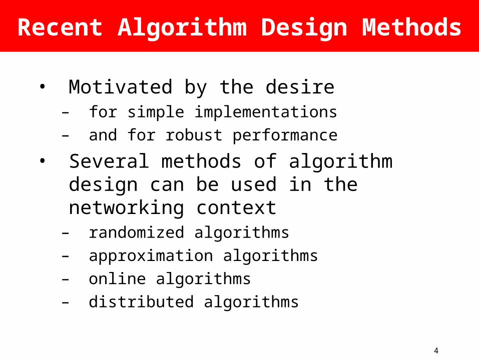
• Motivated by the desire – for simple implementations– and for robust performance
• Several methods of algorithm design can be used in the networking context
– randomized algorithms– approximation algorithms– online algorithms– distributed algorithms

5
In this Mini Course…
• We will consider a number of problems in networking
• Show various methods for algorithm design and for performance analysis

6
Network Layer Functions
• transport packet from sending to receiving hosts
• network layer protocols in every host, router
important functions:• path determination:
route taken by packets from source to dest.
• switching: move packets from router’s input to appropriate router output
networkdata linkphysical
networkdata linkphysical
networkdata linkphysical
networkdata linkphysical
networkdata linkphysical
networkdata linkphysical
networkdata linkphysical
networkdata linkphysical
application
transportnetworkdata linkphysical
application
transportnetworkdata linkphysical

7
The Internet
The Internet Core
Edge Router

Internet Routing Algorithms
High PerformanceSwitching and RoutingTelecom Center Workshop: Sept 4, 1997.
Balaji Prabhakar
9
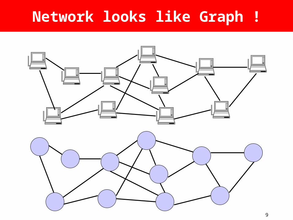
Network looks like Graph !

10
Routing
Graph abstraction for routing algorithms:
• graph nodes are routers
• graph edges are physical links– link cost: delay, $ cost,
or congestion level
Goal: determine “good” path
(sequence of routers) thru network from source to
dest.
Routing protocol
A
ED
CB
F
2
2
13
1
1
2
53
5
• “good” path:– typically means
minimum cost path– other def’s possible

11
Routing Algorithms Classification
Global or decentralized information?
Global:• all routers have complete
topology, link cost info• “link state” algorithmsDecentralized: • router knows physically-
connected neighbors, link costs to neighbors
• iterative process of info exchange with neighbors
• “distance vector” algorithms
Static or dynamic?Static: • routes change slowly
over timeDynamic: • routes change more
quickly– periodic update– in response to link
cost changes

12
Link-State Routing Algorithms: OSPF
Compute least cost paths from a node to all other nodes using Dijkstra’s algorithm.– advertisement carries one entry per neighbor
router– advertisements disseminated via flooding

13
Dijkstra’s algorithm: example
Step012345
start NA
ADADE
ADEBADEBC
ADEBCF
D(B),p(B)2,A2,A2,A
D(C),p(C)5,A4,D3,E3,E
D(D),p(D)1,A
D(E),p(E)infinity
2,D
D(F),p(F)infinityinfinity
4,E4,E4,E
A
ED
CB
F
2
2
13
1
1
2
53
5

14
Route Optimization
Improve user performance and network efficiency by tuning OSPF weights to the prevailing traffic demands.
AT&T
customers orpeers
customers orpeers
backbone

15
Route Optimization
• Traffic engineering – Predict influence of weight changes on traffic flow– Minimize objective function (say, of link utilization)
• Inputs– Networks topology: capacitated, directed graph– Routing configuration: routing weight for each link– Traffic matrix: offered load each pair of nodes
• Outputs– Shortest path(s) for each node pair– Volume of traffic on each link in the graph– Value of the objective function

16
Example
A
B
C
D
1
1 2
1
E
2
Links AB and BD are overloaded
Change weight of CD to 1 to improve routing (load balancing) !

17
References
1. Anja Feldmann, Albert Greenberg, Carsten Lund, Nick Reingold, Jennifer Rexford, and Fred True, "Deriving traffic demands for operational IP networks: Methodology and experience," IEEE/ACM Transactions on Networking, pp. 265-279, June 2001.
2. Bernard Fortz and Mikkel Thorup, "Internet traffic engineering by optimizing OSPF weights," in Proc. IEEE INFOCOM, pp. 519-528, 2000.

18
Distance Vector Routing: RIP
• Based on the Bellman-Ford algorithm– At node X, the distance to Y is updated by
where DX(Y) denote the distance at X currently from X to Y,N(X) is set of the neighbors of node X, and c(X, Z) is the distance of the direct link from X to Z
))(),((min)( )( YDZXcYD ZXNZ
X

19
Distance Table: ExampleA
E D
CB7
8
1
2
1
2
D ()
A
B
C
D
A
0
7
1c(E,A)
B
7
0
1
8c(E,B)
D
2
0
2c(E,D)
E
distance tables from neighbors
dest
inat
ions
A
1
8
B
15
8
9
D
4
2
computation E’sdistance
table
1, A
8, B
4, D
2, D
distance table E sends to its neighbors
A: 1
B: 8
C: 4
D: 2
E: 0
Below is just one step! The algorithm repeats for ever!

20
Link Failure and Recovery
• Distance vectors: exchanged every 30 sec
• If no advertisement heard after 180 sec --> neighbor/link declared dead– routes via neighbor invalidated– new advertisements sent to neighbors– neighbors in turn send out new
advertisements (if tables changed)– link failure info quickly propagates to entire
net
21
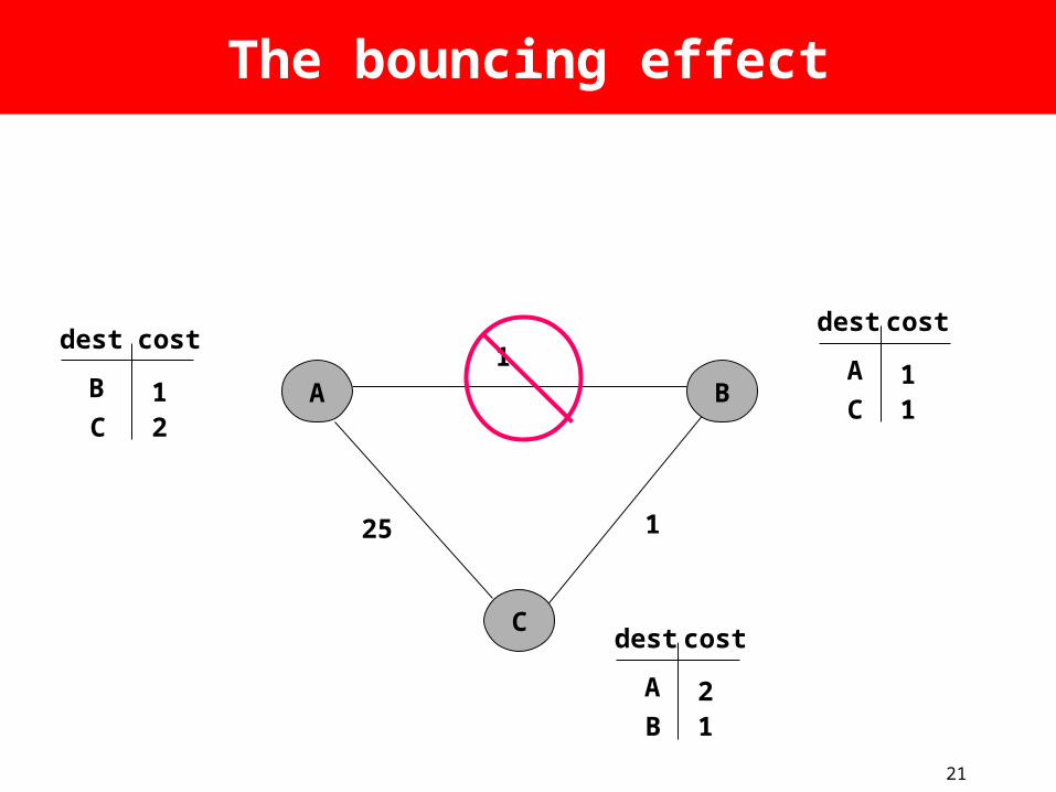
The bouncing effect
A
25
1
1
B
C
B
C 21
dest costA
C 11
dest cost
A
B 12
dest cost

22
C sends routes to B
A
25 1
B
C
B
C 21
dest costA
C 1~
dest cost
A
B 12
dest cost

23
B updates distance to A
A
25 1
B
C
B
C 21
dest costA
C 13
dest cost
A
B 12
dest cost

24
B sends routes to C
A
25 1
B
C
B
C 21
dest costA
C 13
dest cost
A
B 14
dest cost

25
How are these loops caused?
• Observation 1:– B’s metric increases
• Observation 2:– C picks B as next hop to A– But, the implicit path from C to A includes
itself!

26
Solutions
• Split horizon/Poisoned reverse– B does not advertise route to C or advertises it
with infinite distance (16)
• Works for two node loops– does not work for loops with more nodes
27
Example where Split Horizon fails
1
11
1
A B
C
D
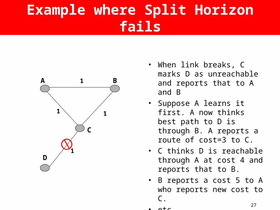
• When link breaks, C marks D as unreachable and reports that to A and B
• Suppose A learns it first. A now thinks best path to D is through B. A reports a route of cost=3 to C.
• C thinks D is reachable through A at cost 4 and reports that to B.
• B reports a cost 5 to A who reports new cost to C.
• etc...

28
Comparison of LS and DV algorithms
Message complexity• LS: with n nodes, E links,
O(nE) msgs sent• DV: exchange between
neighbors only– larger msgs
Speed of Convergence• LS: requires O(nE) msgs
– may have oscillations
• DV: convergence time varies– routing loops– count-to-infinity problem
Robustness: what happens if router malfunctions?
LS: – node can advertise
incorrect link cost– each node computes
only its own table
DV:– DV node can advertise
incorrect path cost– error propagates thru
network

29
Hierarchical Routing
scale: with 50 million destinations:
• can’t store all dest’s in routing tables!
• routing table exchange would swamp links!
administrative autonomy• internet = network of
networks• each network admin may
want to control routing in its own network
Our routing study thus far - idealization • all routers identical• network “flat”… not true in practice
30
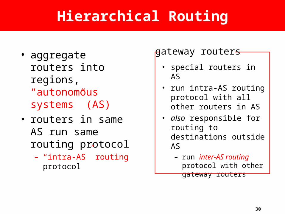
Hierarchical Routing
• aggregate routers into regions, “autonomous systems” (AS)
• routers in same AS run same routing protocol– “intra-AS” routing
protocol
• special routers in AS• run intra-AS routing
protocol with all other routers in AS
• also responsible for routing to destinations outside AS– run inter-AS routing
protocol with other gateway routers
gateway routers

31
Internet AS Hierarchy
Inter-AS border (exterior gateway) routers
Intra-AS interior (gateway) routers

32
Intra-AS and Inter-AS routing
Host h2
a
b
b
aaC
A
Bd c
A.a
A.c
C.bB.a
cb
Hosth1
Intra-AS routingwithin AS A
Inter-AS routingbetween A and B
Intra-AS routingwithin AS B

Peer-to-Peer Networks: Chord
High PerformanceSwitching and RoutingTelecom Center Workshop: Sept 4, 1997.
Balaji Prabhakar

34
A peer-to-peer storage problem
• 1000 scattered music enthusiasts• Willing to store and serve replicas• How do you find the data?

35
The Lookup Problem
Internet
N1
N2 N3
N6N5
N4
Publisher
Key=“title”Value=MP3 data…
ClientLookup(“title”)
?

36
Centralized lookup (Napster)
Publisher@
Client
Lookup(“title”)
N6
N9 N7
DB
N8
N3
N2N1SetLoc(“title”, N4)
Simple, but O(N) state and a single point of failure
Key=“title”Value=MP3 data…
N4

37
Flooded queries (Gnutella)
N4Publisher@
Client
N6
N9
N7N8
N3
N2N1
Robust, but worst case O(N) messages per lookup
Key=“title”Value=MP3 data…
Lookup(“title”)

38
Routed queries (Freenet, Chord, etc.)
N4Publisher
Client
N6
N9
N7N8
N3
N2N1
Lookup(“title”)
Key=“title”Value=MP3 data…

39
Chord Distinguishing Features
•Simplicity•Provable Correctness•Provable Performance

40
Chord Simplicity
• Resolution entails participation by O(log(N)) nodes
• Resolution is efficient when each node enjoys accurate information about O(log(N)) other nodes
41
Chord Algorithms
•Basic Lookup•Node Joins•Stabilization•Failures and Replication

42
Chord Properties
• Efficient: O(log(N)) messages per lookup– N is the total number of servers
• Scalable: O(log(N)) state per node• Robust: survives massive failures

43
Chord IDs
• Key identifier = SHA-1(key)• Node identifier = SHA-1(IP address)• Both are uniformly distributed• Both exist in the same ID space
• How to map key IDs to node IDs?

44
Consistent Hashing[Karger 97]
• Target: web page caching• Like normal hashing, assigns items to
buckets so that each bucket receives roughly the same number of items
• Unlike normal hashing, a small change in the bucket set does not induce a total remapping of items to buckets

45
Consistent Hashing [Karger 97]
N32
N90
N105
K80
K20
K5
Circular 7-bitID space
Key 5Node 105
A key is stored at its successor:node with next higher ID

46
Basic lookup
N32
N90
N105
N60
N10N120
K80
“Where is key 80?”
“N90 has K80”

47
Simple lookup algorithm
Lookup(my-id, key-id)n = my successorif my-id < n < key-id
call Lookup(id) on node n // next hop
elsereturn my successor // done
• Correctness depends only on successors

48
“Finger table” allows log(N)-time lookups
N80
½¼
1/8
1/161/321/641/128
49
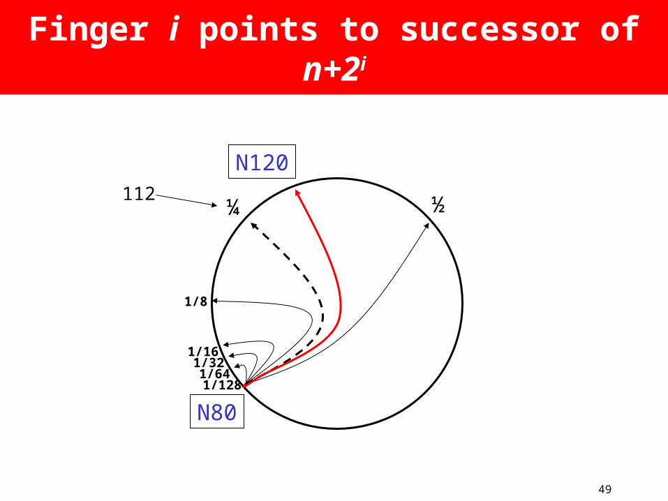
Finger i points to successor of n+2i
N80
½¼
1/8
1/161/321/641/128
112
N120

50
Lookup with fingers
Lookup(my-id, key-id)look in local finger table for
highest node n s.t. my-id < n < key-idif n exists
call Lookup(id) on node n // next hop
elsereturn my successor // done

51
Lookups take O(log(N)) hops
N32
N10
N5
N20
N110
N99
N80
N60
Lookup(K19)
K19

52
Node JoinLinked List Insert
N36
N40
N25
1. Lookup(36)K30K38

53
Node Join (2)
N36
N40
N25
2. N36 sets its ownsuccessor pointer
K30K38

54
Node Join (3)
N36
N40
N25
3. Copy keys 26..36from N40 to N36
K30K38
K30

55
Node Join (4)
N36
N40
N25
4. Set N25’s successorpointer
Update finger pointers in the backgroundCorrect successors produce correct lookups
K30K38
K30

56
Stabilization
• Case 1: finger tables are reasonably fresh• Case 2: successor pointers are correct;
fingers are inaccurate• Case 3: successor pointers are inaccurate
or key migration is incomplete• Stabilization algorithm periodically verifies
and refreshes node knowledge– Successor pointers– Predecessor pointers– Finger tables
57
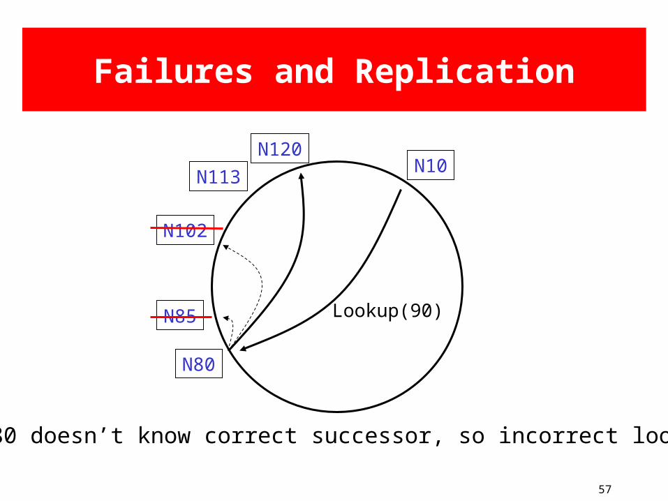
Failures and Replication
N120
N113
N102
N80
N85
N80 doesn’t know correct successor, so incorrect lookup
N10
Lookup(90)

58
Solution: successor lists
• Each node knows r immediate successors• After failure, will know first live successor• Correct successors guarantee correct lookups
• Guarantee is with some probability

59
Choosing the successor list length
• Assume 1/2 of nodes fail• P(successor list all dead) = (1/2)r
– I.e. P(this node breaks the Chord ring)– Depends on independent failure
• P(no broken nodes) = (1 – (1/2)r)N
– r = 2log(N) makes prob. = 1 – 1/N

60
References
Ion Stoica, Robert Morris, David Liben-Nowell, David R. Karger, M. Frans Kaashoek, Frank Dabek, Hari Balakrishnan, ``Chord: A Scalable Peer-to-peer Lookup Protocol for Internet Applications,'‘IEEE/ACM Transactions on Networking, Vol. 11, No. 1, pp. 17-32, February 2003.

Switch Scheduling Algorithms
High PerformanceSwitching and RoutingTelecom Center Workshop: Sept 4, 1997.
Balaji Prabhakar

62
Basic Architectural Components
ForwardingDecision
ForwardingDecision
ForwardingDecision
RoutingTable
RoutingTable
RoutingTable
Interconnect
OutputScheduling
1.
2.
3.

63
Switching Fabrics
Output Queued
InputQueued
Combined Input and
Output Queued ParallelPacket
Switches37526014
72356104
75231064
70513426
74560312
76453202
76543210
000001
010011
100101
110111
Batcher Sorter Self-Routing Network
Multistage

64
Input Queueing
configuration
Data
In
Data Out
Scheduler

65
Background
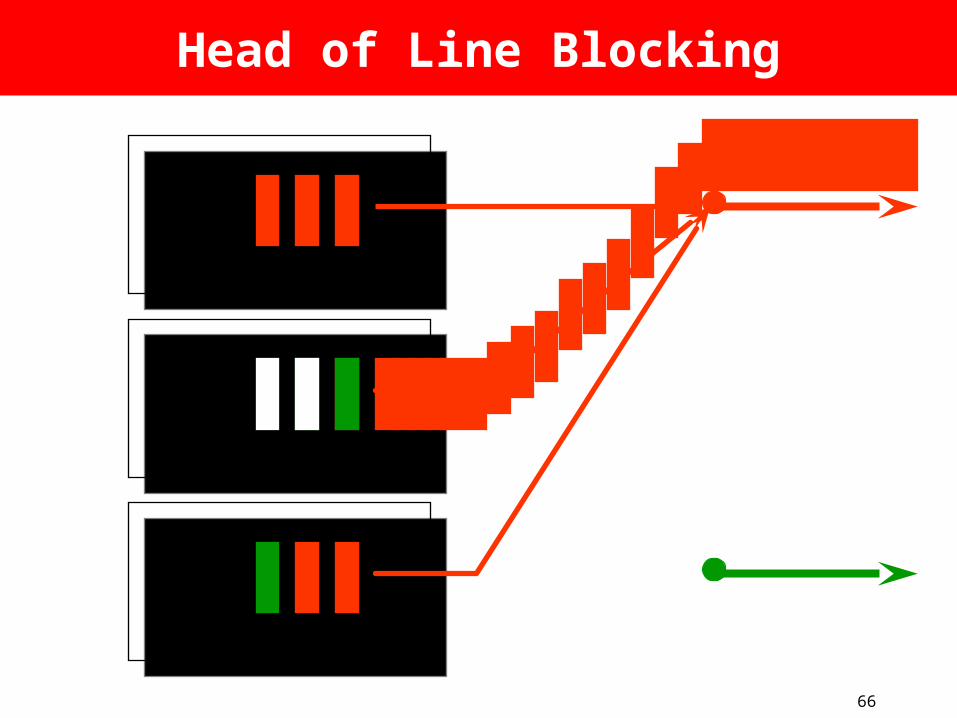
1. [Karol et al. 1987] Throughput limited to by head-of-line blocking for Bernoulli IID uniform traffic.
2. [Tamir 1989] Observed that with “Virtual Output Queues” (VOQs) Head-of-Line blocking is reduced and throughput goes up.
%5822
66
Head of Line Blocking

67

68

69
Input QueueingVirtual output queues

70
Background Scheduling via Matching
3. [Anderson et al. 1993] Observed analogy to maximum size matching in a bipartite graph.
4. [McKeown et al. 1995] (a) Maximum size match can not guarantee 100% throughput.(b) But maximum weight match can – O(N3).
Matching
O(N2.5)

71
BackgroundSpeedup
5. [Chuang, Goel et al. 1997] Precise emulation of a central shared memory switch is possible with a speedup of two and a “stable marriage” scheduling algorithm.
6. [Prabhakar and Dai 2000] 100% throughput possible for maximal matching with a speedup of two.

72
Simulation
Input Queueing Output Queueing

73
Using Speedup
1
1
1
2
2

74
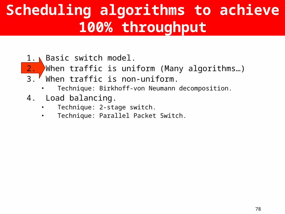
Scheduling algorithms to achieve 100% throughput
1. Basic switch model.2. When traffic is uniform (Many algorithms…)3. When traffic is non-uniform.
• Technique: Birkhoff-von Neumann decomposition.
4. Load balancing.• Technique: 2-stage switch.• Technique: Parallel Packet Switch.
75
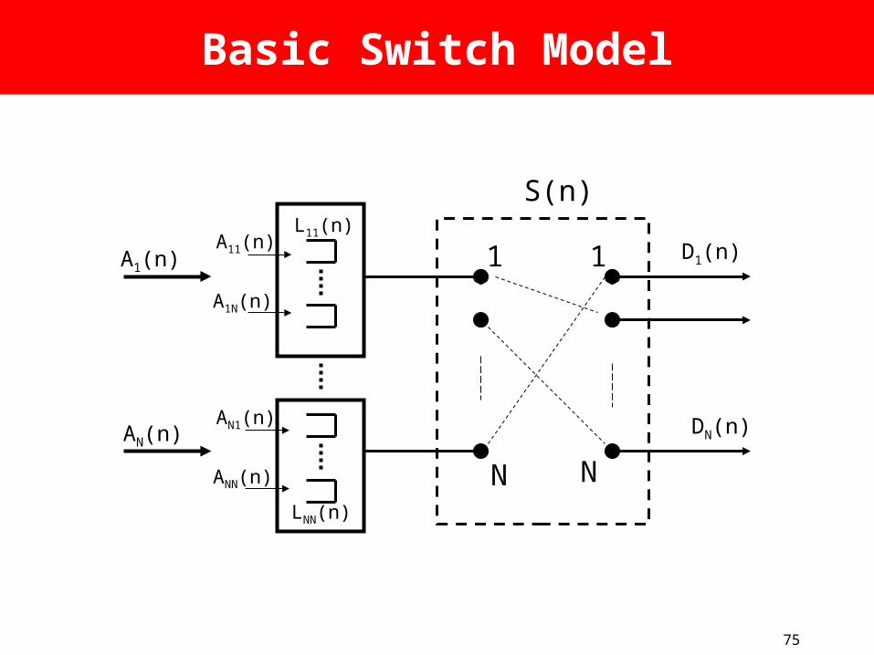
Basic Switch Model
A1(n)
S(n)
N NLNN(n)
A1N(n)
A11(n)L11(n)
1 1
AN(n)
ANN(n)
AN1(n)
D1(n)
DN(n)

76
Some Definitions
matrix. npermutatio a is and :where
:matrix Service 2.
".admissible" is traffic the say we If
where
:matrix Traffic 1.
SssS
nAE
ijij
jij
iij
ijijij
1,0],[
1,1
)]([:,
3. Queue occupancies:
Occupancy
L11(n) LNN(n)

77
Some possible performance goals
?metrics... Other 6
5
4
3.
"throughput "100% 2.
onconservati Work 1.
.
)(lim
)(lim.
,)]([.
,)(
ij
ij
n
ij
n
ij
ij
n
nA
n
nD
CnLE
nCnL
When traffic is
admissible
78
Scheduling algorithms to achieve 100% throughput
1. Basic switch model.2. When traffic is uniform (Many algorithms…)3. When traffic is non-uniform.
• Technique: Birkhoff-von Neumann decomposition.
4. Load balancing.• Technique: 2-stage switch.• Technique: Parallel Packet Switch.

79
Algorithms that give 100% throughput for uniform traffic
• Quite a few algorithms give 100% throughput when traffic is uniform
• “Uniform”: the destination of each cell is picked independently and uniformly and at random (uar) from the set of all outputs.

80
Maximum size bipartite match
• Intuition: maximizes instantaneous throughput
• Gives 100% throughput for uniform traffic.
L11(n)>0
LN1(n)>0
“Request” Graph Bipartite Match
MaximumSize Match

81
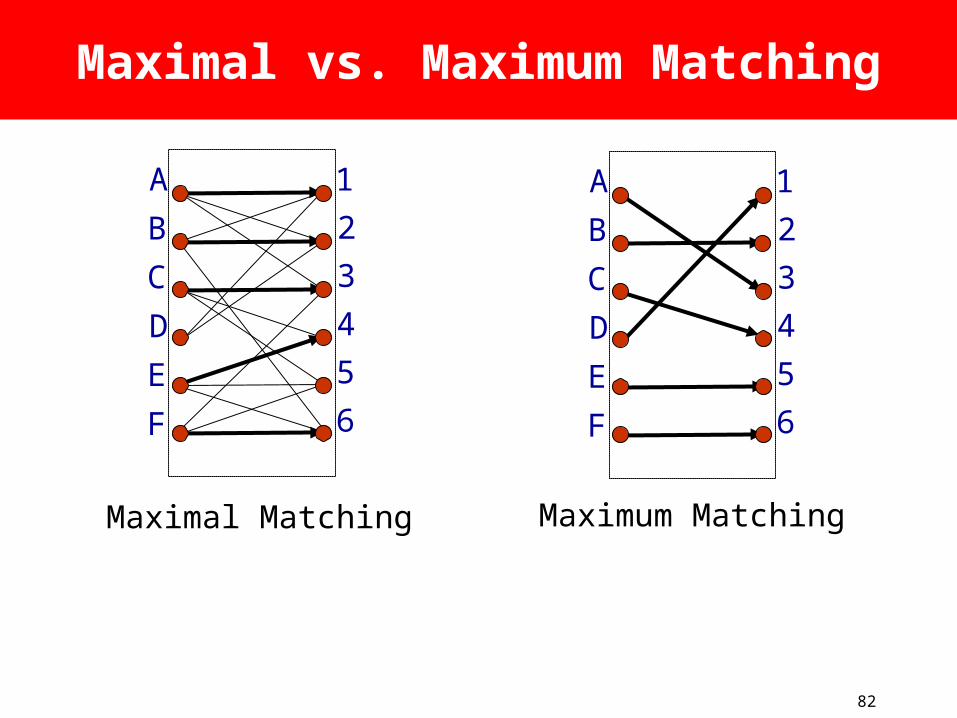
Some Observations
• A maximum size match (MSM) maximizes instantaneous throughput.
• But a MSM is complex – O(N2.5).• In general, maximal matching is much
simpler to implement, and has a much faster running time.
• A maximal size matching is at least half the size of a maximum size matching.
82
Maximal vs. Maximum Matching
A 1
B
C
D
E
F
2
3
4
5
6
A 1
B
C
D
E
F
2
3
4
5
6
Maximal Matching Maximum Matching

83
TDM Scheduling Algorithm
If arriving traffic is i.i.d with destinations picked uar across outputs, then a “TDM” schedule gives 100% throughput.
A 1
B
C
D
2
3
4
B
C
D
2
3
4
B
C
D
2
3
4
A 1 A 1
Permutations are picked uar from the set of N! permutations.

84
Why doesn’t maximizing instantaneous throughput give 100% throughput for non-
uniform traffic?
2/1
2/1
2/1
32
21
1211Three possiblematches, S(n):
100%). t(throughpu stable not is switch 0.0358 if so And
But
most at is served is 1 input which at rate total The
. w.p. serviced is 1 Input ) w.p.( arrivals have
both and and , time at that Assume
.)21(31121
.)21(311
)21(11)21(32
32)21(
)()(0)(0)(
21
2
22
2
32211211
-δ// - -λ
//
/-//
/-δ/
nQnQ n, L nn, L

85
Scheduling algorithms to achieve 100% throughput
1. Basic switch model.2. When traffic is uniform (Many algorithms…)3. When traffic is non-uniform.
• Technique: Birkhoff-von Neumann decomposition.
4. Load balancing.• Technique: 2-stage switch.• Technique: Parallel Packet Switch.

86
Example:With random arrivals, but known traffic matrix
• Assume we know the traffic matrix, and the arrival pattern is random:
• Then we can simply choose:
1000
0100
002/12/1
002/12/1
1000
0100
0001
0010
)(,
1000
0100
0010
0001
)( evenSoddS

87
Birkhoff - von Neumann Decomposition
rate. arrival the exceeds rate
departure the and words, other In
is period in of soccurrence of# the that So
:matrices service of sequence the pick Then
element) by (element
:that such matrices, service of set and
constants of set some pick can we y,Intuitivel
,0))((
.
),,,,,,,()(
.,
),(
),,(
1
13221
1
1
1
T
i
ii
r
r
iii
r
r
iS
aTM
T
MMMMMMnS
Ma
MM
aa
Turns out, any can always be decomposed into a linear (convex) combination of matrices, (M1, …, Mr) by Birkhoff-von Neumann.

88
Birkhoff ‘1946 Decomposition Example
4.05.01.0
5.02.03.0
1.03.06.0~R
2.05.01.0
5.003.0
1.03.04.0
100
010
001
= 0.2 +
=
010
100
001
0.40.2
100
010
001
+
2.01.01.0
1.003.0
1.03.00
+
010
001
100
1.0
001
100
010
1.0
100
001
010
2.0
010
100
001
4.0
100
010
001
2.0~R

89
In practice…
• Unfortunately, we usually don’t know traffic matrix a priori, so we can:– measure or estimate , or– use the current queue occupancies.

90
Scheduling algorithms to achieve 100% throughput
1. Basic switch model.2. When traffic is uniform (Many algorithms…)3. When traffic is non-uniform.
• Technique: Birkhoff-von Neumann decomposition.
4. Load balancing.• Technique: 2-stage switch.• Technique: Parallel Packet Switch.

91
2-stage Switch
Motivation:1. If traffic is uniformly distributed, then
even a simple TDM schedule gives 100% throughput.
2. So why not force non-uniform traffic to be uniformly distributed?

92
2-stage Switch
S2(n)
N NLNN(n)
L11(n)
1 1 D1(n)
DN(n)
N N
1 1 A’1(n)
A’N(n)
S1(n)
A1(n)
AN(n)
BufferlessLoad-balancing
Stage
BufferedSwitching
Stage

93
2-stage Switch
ˆ( ) ,
ˆ mod
nn
n n N
1. Consider a periodic sequence of permutation matrices:
where is a one-cycle permutation matrix
(f or example, a TDM sequence), and .
2. I f 1st stage is
Main Result [Chang et al.]:
1 1
1
2 2
( ) ( ),
( ) ( ),
n n
n n
scheduled by a sequence of permutation
matrices:
where is a random starting phase, and
3. The 2nd stage is scheduled by a sequence of permutation
matrices:
4. Then the switch gives 100% throughput f or a very broad
range of traffi c types.
1st stage makes non-unif orm traffi c unif orm,
and breaks up burstiness. For bursty traffi c, delay can be
lower than f or an ou
Observation 1:
tput queued switch!
Cells can become mis-sequenced.Observation 2:

94
Parallel Packet Switches
Definition:
A PPS is comprised of multiple identical lower-speed packet-switches operating independently and in parallel. An incoming stream of packets is spread, packet-by-packet, by a demultiplexor across the slower packet-switches, then recombined by a multiplexor at the output.
We call this “parallel packet switching”

95
Architecture of a PPS
OQ Switch
OQ Switch
OQ Switch
1
2
3
N=4
R
R
R
R
1
2
3
N=4
R
R
R
R
MultiplexorDemultiplexor
Demultiplexor
Demultiplexor
Demultiplexor
Multiplexor
Multiplexor
Multiplexor
(sR/k) (sR/k)
k=3
1
2
(sR/k) (sR/k)

96
Parallel Packet SwitchesResults
[Iyer et al.] If S >= 2 then a PPS can precisely emulate a FIFO output queued switch for all traffic patterns, and hence achieves 100% throughput.

97
References
1. C.-S. Chang, W.-J. Chen, and H.-Y. Huang, "Birkhoff-von Neumann input buffered crossbar switches," in Proceedings of IEEE INFOCOM '00, Tel Aviv, Israel, 2000, pp. 1614 – 1623.
2. N. McKeown, A. Mekkittikul, V. Anantharam, and J. Walrand. Achieving 100% Throughput in an Input-Queued Switch. IEEE Transactions on Communications, 47(8), Aug 1999.
3. A. Mekkittikul and N. W. McKeown, "A practical algorithm to achieve 100% throughput in input-queued switches," in Proceedings of IEEE INFOCOM '98, March 1998.
4. L. Tassiulas, “Linear complexity algorithms for maximum throughput in radio networks and input queued switchs,” in Proc. IEEE INFOCOM ‘98, San Francisco CA, April 1998.
5. C.-S. Chang, D.-S. Lee, Y.-S. Jou, “Load balanced Birkhoff-von Neumann switches,” Proceedings of IEEE HPSR ‘01, May 2001, Dallas, Texas.
6. S. Iyer, N. McKeown, "Making parallel packet switches practical," in Proc. IEEE INFOCOM `01, April 2001, Alaska.

Competitive Analysis: Theory and Applications in Networking
High PerformanceSwitching and RoutingTelecom Center Workshop: Sept 4, 1997.
Balaji Prabhakar

99
Decision Making Under Uncertainty:
Online Algorithms and Competitive Analysis
• Online Algorithm:– Inputs arrive online (one by one)– Algorithm must process each input as it arrives– Lack of knowledge of future arrivals results in
inefficiency
• Malicious, All-powerful Adversary:– Omniscient: monitors the algorithm– Generates “worst-case” inputs
• Competitive Ratio:– Worst ratio of the “cost” of online algorithm to
the “cost” of optimum algorithm

100
Competitive Analysis: Discussion
• Very Harsh Model– All powerful adversary
• But..– Can often still prove good competitive ratios– Really tough Testing-Ground for Algorithms– Often leads to good rules of thumb which can
be validated by other analyses– Distribution independent: doesn’t matter
whether traffic is heavy-tailed or Poisson or Bernoulli

101
Competitive Analysis in Networking: Outline
• Shared Memory Switches• Multicast Trees
– The Greedy Strategy
• Routing and Admission Control– The Exponential Metric
• More Restricted Adversaries– Adversarial Queueing Theory
• Congestion Control
102
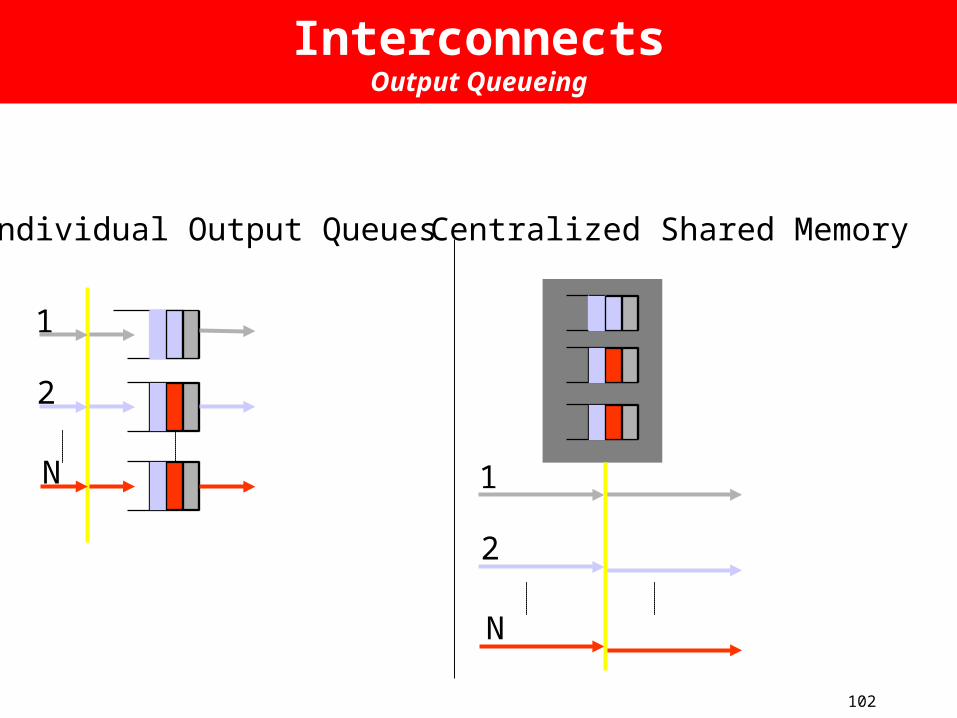
InterconnectsOutput Queueing
Individual Output Queues Centralized Shared Memory
1
2
N 1
2
N

103
Buffer Model
• We consider NxN switch• Shared memory able to hold M bytes• Packets may be either:
– accepted/rejected– preempted
• All packets have the same size
M

104
Shared Memory Example

105
Competitive Analysis
Aim: maximize the total number of packets transmitted
For each packet sequence S denote,• VOPT(S): value of best possible solution,
• VA(S): value obtained by algorithm A
Throughput-Competitive Ratio: MAXS {VOPT(S) / VA(S)}
Uniform performance guarantee

106
Longest Queue Drop Policy
When a packet arrives:– Always accept if the buffer is not full– Otherwise we accept the packet and drop
a packet from the tail of the longest queue

107
Longest Queue Drop Policy
M = 9

108
LQD Policy Analysis
Theorem 1 (UB): The competitive ratio of the LQD Policy is at most 2.
Theorem 2 (LB): The competitive ratio of the LQD policy is at least 2.
Theorem 3 (LB): The competitive ratio of any online policy is at least 4/3.

109
Proof Outline (UB)
EXTRA
OPT LQD
Definition: An OPT packet p sent at time t is an extra packet if the LQD port is idle.
Claim: There exists a matching between each packet from EXTRA to a packet in LQD.

110
Matching Construction
• For each unmatched OPT packet p in a higher position than the LQD queue length:
• When p arrives and it is accepted by both OPT and LQD then match p to itself • Otherwise, match p to any unmatched packet in LQD
• If a matched LQD packet p is preempted, then the preempting packet replaces p.

111
Proof Outline (UB)
OPT LQD
112
Proof Outline (UB)
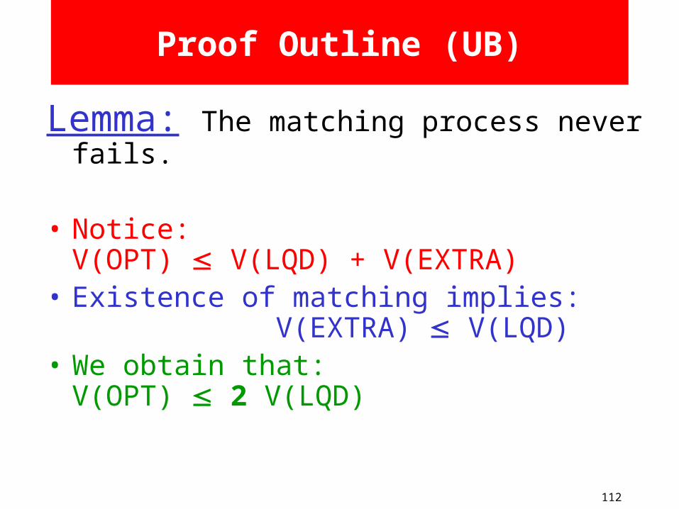
Lemma: The matching process never fails.
• Notice:V(OPT) V(LQD) + V(EXTRA)
• Existence of matching implies:V(EXTRA) V(LQD)
• We obtain that:V(OPT) 2 V(LQD)

113
Proof Outline (LB)
Scenario (active ports 1 & 2):
• At t = 0 two bursts of M packets to 1 & 2 arrive. • The online retains at most M/2, say 1’s packets.• During the following M time slots one packet destined to 2 arrives. • The scenario is repeated.

114
Proof Outline (LB-LQD)
Scenario:
• the switch memoryM = A2/2 + A
• the number of output ports N = 3A
AActive
Ovld.
IdleA
A

115
Proof Outline (LB-LQD)
Active output ports: • have an average load of 1 with period A • the bursts to successive ports are evenly staggered in time
Overloaded output ports: • receive exactly 2 packets every time slot
116
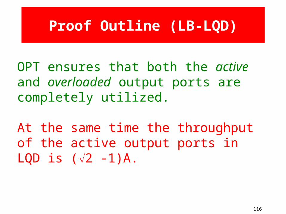
Proof Outline (LB-LQD)
OPT ensures that both the active and overloaded output ports are completely utilized.
At the same time the throughput of the active output ports in LQD is (2 -1)A.
117
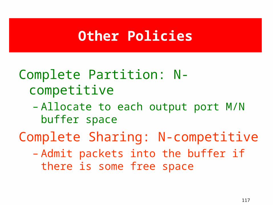
Other Policies
Complete Partition: N-competitive– Allocate to each output port M/N buffer
space
Complete Sharing: N-competitive– Admit packets into the buffer if there is
some free space

118
Other Policies Cont.
Static Threshold: N-competitive– Set the threshold for a queue length to M/N– A packet is admitted if the threshold is not
violated and there is a free space
Dynamic Threshold: open problem– Set the threshold for a queue length to the
amount of the free buffer space– All packets above the threshold are rejected

119
Competitive Analysis in Networking: Outline
• Shared Memory Switches• Multicast Trees
– The Greedy Strategy
• Routing and Admission Control– The Exponential Metric
• More Restricted Adversaries– Adversarial Queueing Theory
• Congestion Control
120
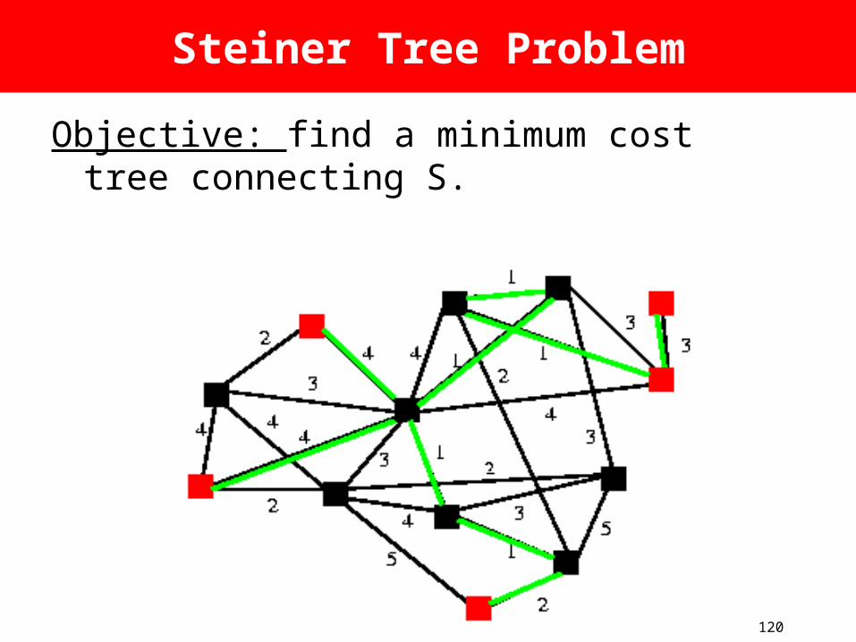
Steiner Tree Problem
Objective: find a minimum cost tree connecting S.

121
• Step 1: Construct a complete directed distance graph G1=(V1,E1,c1).
• Step 2: Find the min spanning tree T1 of G1.
• Step3: Construct a subgraph GS of G by replacing each edge in T1 by its corresponding shortest path in G.
• Step 4: Find the min spanning tree TS of GS.
• Step 5: Construct a Steiner tree TH from TS by deleting edges in TS if necessary, so that all the leaves in TH are Steiner points.
KMB Algorithm (Offline)Due to [Kou, Markowsky and Berman 81’]

122
Worst case time complexity O(|S||V|2).
Cost no more than 2(1 - 1/l) *optimal cost where l = number of leaves in the steiner
tree.
KMB Algorithm Cont.

123
KMB Example
A
C
D4
4
444 4
B
A
C
D4
4
4
B
A
B
C D
EF
G
HI
10
1
1
2
9
8
1 1
1/2
2
1/2
1
B
C D
EF
G
HI
1
1
2
1 1
1/2
2
1/2
1
A
Destination Nodes
Intermediate Nodes

124
KMB Example Cont.
B
C D
EF
G
HI
1
1
2
1 1
1/2
2
1/2
A
B
C D
EF
I
1
1
2
1 1
2
A
Destination Nodes
Intermediate Nodes

125
Incremental Construction of Multicast Trees
• Fixed Multicast Source s– K receivers arrive one by one– Must adapt multicast tree to each new arrival
without rerouting existing receivers– Malicious adversary generates bad requests– Objective: Minimize total size of multicast tree
s r1
a
b
r1r1
bb
C=3/2
Can create worse sequences

126
Dynamic Steiner Tree (DST)
• G=(V,E) weighted, undirected, connected graph.
• Si V is the set of terminal nodes to be connected at step i.
127
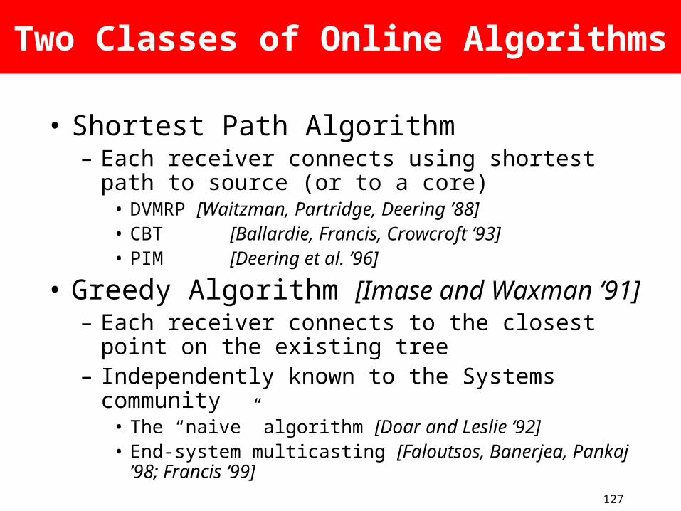
Two Classes of Online Algorithms
• Shortest Path Algorithm– Each receiver connects using shortest path to
source (or to a core)• DVMRP [Waitzman, Partridge, Deering ’88]• CBT [Ballardie, Francis, Crowcroft ‘93]• PIM [Deering et al. ’96]
• Greedy Algorithm [Imase and Waxman ‘91]– Each receiver connects to the closest point on
the existing tree– Independently known to the Systems community
• The “naive” algorithm [Doar and Leslie ‘92]• End-system multicasting [Faloutsos, Banerjea, Pankaj
’98; Francis ‘99]

128
Shortest Path Algorithm: Example
• Receivers r1, r2, r3, … , rK join in order
N
s
r1
r2
r3
rK

129
Shortest Path Algorithm
• Cost of shortest path tree K N
N
s
r1
r2
r3
rK

130
Shortest Path AlgorithmCompetitive Ratio
• Optimum Cost K + N• If N is large, the competitive ratio is K
s
r1
r2
r3
rK

131
Greedy Algorithm
• Theorem 1: For the greedy algorithm, competitive ratio = O(log K)
• Theorem 2: No algorithm can achieve a competitive ratio better than log K
[Imase and Waxman ’91]
Greedy algorithm is the optimum strategy

132
Proof of Theorem 1
[Alon and Azar ’93]
• L = Size of the optimum multicast tree
• pi = amount paid by online algorithm for ri
– i.e. the increase in size of the greedy multicast tree as a result of adding receiver ri
• Lemma 1: The greedy algorithm pays 2L/j or more for at most j receivers– Assume the lemma– Total Cost 2L (1 + 1/2 + 1/3 + … 1/K) ¼ 2L
log K

133
Proof of Lemma 3
Suppose towars a contradiction that there are more than j receivers for which the greedy algorithm paid more than 2L/j– Let these be r1, r2, … , rm, for m larger than j
– Each of these receivers is at least 2L/j away from each other and from the source

134
rm
Tours and Trees
s
r1 r2
r3
r4
Each segment 2L/j,Tour cost > 2L
s
r1 r2r3
r4
rm
One can construct tour from tree by repeating edges at most twice, Tour cost 2L

135
Competitive Analysis in Networking: Outline
• Shared Memory Switches• Multicast Trees
– The Greedy Strategy
• Routing and Admission Control– The Exponential Metric
• More Restricted Adversaries– Adversarial Queueing Theory
• Congestion Control

136
The Exponential Cost Metric
• Consider a resource with capacity C• Assume that a fraction of the resource has
been consumed• Exponential cost “rule of thumb”: The cost of the
resource is given by for appropriately chosen • Intuition: Cost increases steeply with
– Bottleneck resources become expensive
Cost

137
Applications of Exponential Costs
• Exponential cost “rule of thumb” applies to– Online Routing– Online Call Admission Control– Stochastic arrivals– Stale Information– Power aware routing

138
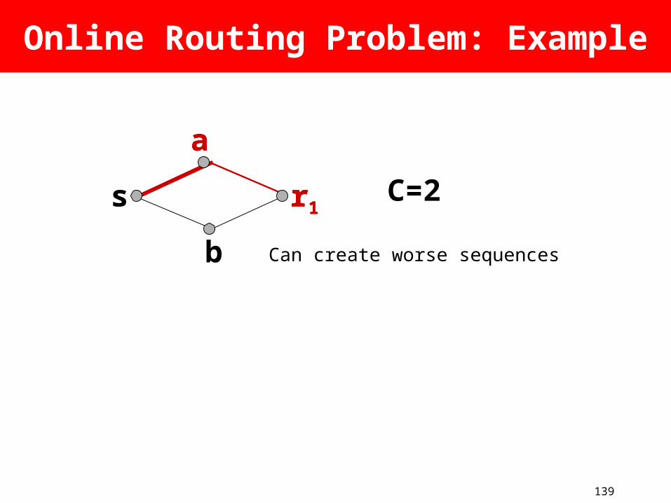
The Online Routing Problem
• Connection establishment requests arrive online in a VPN (Virtual Private Network)
• Must assign a route to each connection and reserve bandwidth along that route– PVCs in ATM networks– MPLS + RSVP in IP networks
• Oversubscribing is allowed– Congestion = the worst oversubscribing on a link
• Goal: Assign routes to minimize congestion• Assume all connections have identical b/w
requirement, all links have identical capacity
139
Online Routing Problem: Example
s r1
b
r1r1C=2
Can create worse sequences
aaa

140
Online Algorithm for Routing
• L = Fraction of bandwidth of link L that has been already reserved
• = N, the size of the network
• The Exponential Cost Algorithm:– Route each incoming connection on current
cheapest path from src to dst– Reserve bandwidth along this path[Aspnes et al. ‘93]
141
Online Algorithm for Routing
• Theorem 1: The exponential cost algorithm achieves a competitive ratio of O(log N) for congestion
• Theorem 2: No algorithm can achieve competitive ratio better than log N in asymmetric networks
This simple strategy is optimum!

142
Applications of Exponential Costs
• Exponential cost “rule of thumb” applies to– Online Routing– Online Call Admission Control– Stochastic arrivals– Stale Information– Power aware routing

143
Online Admission Control and Routing
• Connection establishment requests arrive online
• Must assign a route to each connection and reserve bandwidth along that route
• Oversubscribing is not allowed– Must perform admission control
• Goal: Admit and route connections to maximize total number of accepted connections (throughput)

144
Exponential Metric and Admission Control
• When a connection arrives, compute the cheapest path under current exponential costs
• If the cost of the path is less than then accept the connection; else reject[Awerbuch, Azar, Plotkin ’93]
• Theorem: This simple algorithm admits at least O(1/log N) as many calls as the optimum

145
Applications of Exponential Costs
• Exponential cost “rule of thumb” applies to– Online Routing– Online Call Admission Control– Stochastic arrivals– Stale Information– Power aware routing
146
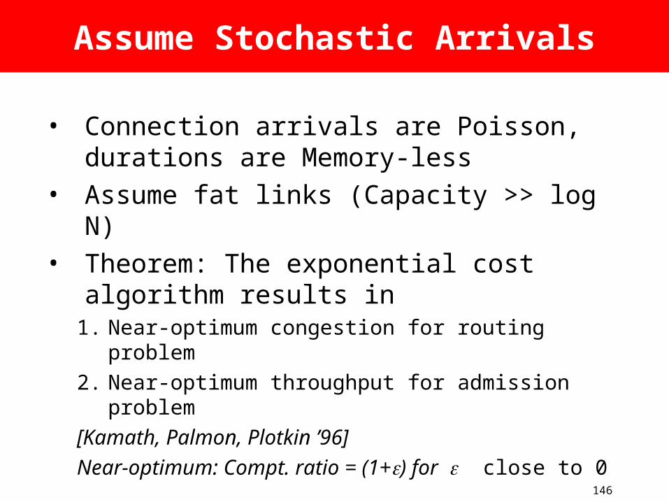
Assume Stochastic Arrivals
• Connection arrivals are Poisson, durations are Memory-less
• Assume fat links (Capacity >> log N)• Theorem: The exponential cost
algorithm results in1. Near-optimum congestion for routing problem 2. Near-optimum throughput for admission
problem[Kamath, Palmon, Plotkin ’96]Near-optimum: Compt. ratio = (1+) for close
to 0

147
Versatility of Exponential Costs
• Guarantees of log N for Competitive ratio against malicious adversary
• Near-optimum for stochastic arrivals• Near-optimum given fixed traffic matrix
[Young ’95; Garg and Konemann ’98]

148
Applications of Exponential Costs
• Exponential cost “rule of thumb” applies to– Online Routing– Online Call Admission Control– Stochastic arrivals– Stale Information– Power aware routing
149
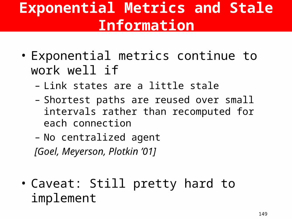
Exponential Metrics and Stale Information
• Exponential metrics continue to work well if– Link states are a little stale– Shortest paths are reused over small intervals
rather than recomputed for each connection– No centralized agent[Goel, Meyerson, Plotkin ’01]
• Caveat: Still pretty hard to implement

150
Applications of Exponential Costs
• Exponential cost “rule of thumb” applies to– Online Routing– Online Call Admission Control– Stochastic arrivals– Stale Information– Power aware routing

151
Power Aware Routing
• Consider a group of small mobile nodes eg. sensors which form an adhoc network– Bottleneck Resource: Battery– Goal: Maximize the time till the network partitions
• Assign a cost to each mobile node which is where = fraction of battery consumed– Send packets over the cheapest path under this cost
measure
• O(log n) competitive against an adversary– Near-optimum for stochastic/fixed traffic

152
Competitive Analysis in Networking: Outline
• Shared Memory Switches• Multicast Trees
– The Greedy Strategy
• Routing and Admission Control– The Exponential Metric
• More Restricted Adversaries– Adversarial Queueing Theory
• Congestion Control

153
• Malicious, all-knowing adversary– Injects packets into the network– Each packet must travel over a specified route
• Suppose adversary injects 3 packets per second from s to r– Link capacities are one packet per second
– No matter what we do, we will have unbounded queues and unbounded delays
– Need to temper our definition of adversaries
Adversarial Queueing TheoryMotivation
sr

154
Adversarial Queueing TheoryBounded Adversaries
• Given a window size W, and a rate r < 1– For any link L, and during any interval of
duration T > W, the adversary can inject at most rT packets which have link L in their route
• Adversary can’t set an impossible task!!– More gentle than competitive analysis
• Will study packet scheduling strategies– Which packet to forward if more than one
packets are waiting to cross a link?

155
Some Interesting Scheduling Policies
• FIFO: First In First Out• LIFO: Last In First Out• NTG: Nearest To Go
– Forward a packet which is closest to destination
• FTG: Furthest To Go– Forward a packet which is furthest from its destination
• LIS: Longest In System– Forward the packet that got injected the earliest– Global FIFO
• SIS: Shortest In System– Forward the packet that got injected the last– Global LIFO

156
Stability in the Adversarial Model
• Consider a scheduling policy (eg. FIFO, LIFO etc.)
• The policy is universally stable if for networks and all “bounded adversaries”, the packet delays and queue sizes remain bounded
• FIFO, LIFO, NTG are not universally stable [Borodin et al. ‘96]
• LIS, SIS, FTG are universally stable[Andrews et al. ‘96]

157
Adversarial Queueing Model: Routing
Using the Exponential Cost Metric
• Adversary injects packets into the network but gives only the src, dst– The correct routes are hidden
• Need to compute routes– Again, use the exponential cost metric– Reset the cost periodically to zero– Use any stable scheduling policy
• Theorem: The combined routing and scheduling policy is universally stable[Andrews et al. ’01]
158
Competitive Analysis in Networking: Outline
• Shared Memory Switches• Multicast Trees
– The Greedy Strategy
• Routing and Admission Control– The Exponential Metric
• More Restricted Adversaries– Adversarial Queueing Theory
• Congestion Control
159
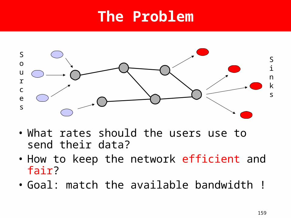
The Problem
• What rates should the users use to send their data?
• How to keep the network efficient and fair?
• Goal: match the available bandwidth !
Sources
Sinks

160
Model Description
• Model– Time divided into steps– Oblivious Adversary– Source select xi
• Severe cost function
Time
Available Bandwidth bichosen by the Adversary
Algorithm picks and sends xi

161
Competitive Ratio
• An Algorithm achieves
• Optimal (offline) achieves
• Seek to minimize

162
Adversary Model
• Unrestricted Adversary– Has too much power
• Fixed Range Adversary
• µ-multiplicative adversary
• {α,β}-additive adversary
163
Fixed Range Model
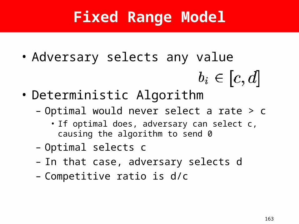
• Adversary selects any value
• Deterministic Algorithm– Optimal would never select a rate > c
• If optimal does, adversary can select c, causing the algorithm to send 0
– Optimal selects c– In that case, adversary selects d– Competitive ratio is d/c

164
Fixed range – Randomized Algorithm
• No randomized algorithm can achieve competitive ratio better than 1+ln(d/c) in the fixed range model with range [c,d]
• Proof :– Yao’s minimax principle– Consider a randomized adversary against
deterministic algorithms– Adversary can choose g(y) = c/y^2 in [c,d)– With probability c/d chooses d
165
Proof continued ….
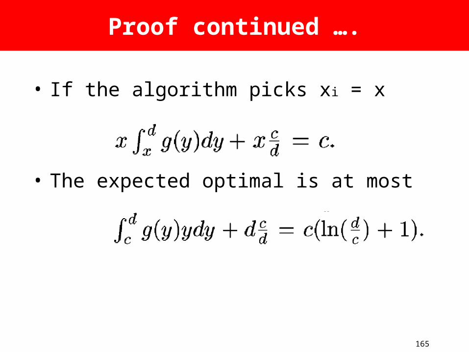
• If the algorithm picks xi = x
• The expected optimal is at most

166
µ-multiplicative model – Randomized Algorithm
• No randomized algorithm can achieve competitive ratio better than ln(µ) + 1
• Proof:– Adversary can always choose bi in [bi, µbi]

167
Randomized Algorithm 4 log(µ) + 12
• Assumptions –relaxed later-– µ is a power of 2– b1 is in the range [1,2µ)
• Algorithm (MIMD)– At step 1, pick at random x1 power of 2
between 1 and 2µ– On failure, xi+1 = xi/2;
– On success, xi+1 = 2µxi;
• Claim:– Competitive ratio of 4 log(µ) + 12

168
Proof outline
• Think about choosing one deterministic algorithm from log(2µ) + 1 choices
• Think about the algorithms as an ensemble running in parallel
• Will show that the ensemble manages to send at least opt/4. [A bit of work]
• Once this is done, picking one algorithm gives opt/4(log(µ)+2)
169
Proof (1/3)
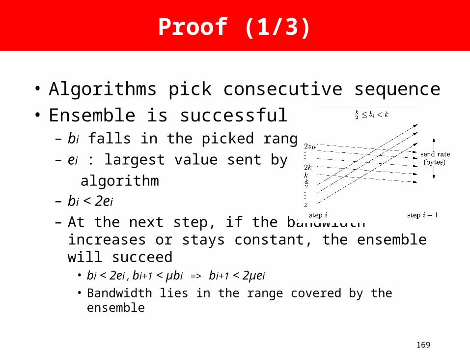
• Algorithms pick consecutive sequence• Ensemble is successful
– bi falls in the picked range– ei : largest value sent by any algorithm – bi < 2ei
– At the next step, if the bandwidth increases or stays constant, the ensemble will succeed
• bi < 2ei , bi+1 < µbi => bi+1 < 2µei
• Bandwidth lies in the range covered by the ensemble

170
Proof (2/3)
• Need to worry about decreasing bandwidth– May decrease very fast– Ensemble achieved ei at step i– Now it was unsuccessful at step i + 1
• Could not have been more than ei available
– At step i+2, they all divide their rates by 2• Could not have been more than ei/2 available
– By induction, one can show that :• ei + ei/2 + ei/4 + …. = 2ei

171
Proof (3/3)
• Optimal algorithm could have achieved at most 4ei
– Up to 2ei in at step I because it is not constrained to choose a power of 2
– 2ei when the ensemble were not successful
• Summing over all time steps, at least we can transmit opt/4
• µ- assumption -> round µ to the next power of 2. Result in log(µ) + 3 algorithms

172
References
1. N. Alon and Y. Azar. On-line Steiner trees in the Euclidean plane. Discrete and Computational Geometry, 10(2), 113-121, 1993.
2. M. Andrews, B. Awerbuch, A. Fernandez, J. Kleinberg, T. Leighton, and Z. Liu. Universal stability results for greedy contention-resolution protocols. Proceedings of the 37th IEEE Conference on Foundations of Computer Science, 1996.
3. M. Andrews, A. Fernandez, A. Goel, and L. Zhang. Source Routing and Scheduling in Packet Networks. To appear in the proceedings of the 42nd IEEE Foundations of Computer Science, 2001.
4. J. Aspnes, Y. Azar, A. Fiat, S. Plotkin, and O. Waarts. On-line load balancing with applications to machine scheduling and virtual circuit routing. Proceedings of the 25th ACM Symposium on Theory of Computing, 1993.
5. B. Awerbuch, Y. Azar, and S. Plotkin. Throughput competitive online routing. Proceedings of the 34th IEEE symposium on Foundations of Computer Science, 1993.
6. A. Ballardie, P. Francis, and J. Crowcroft. Core Based Trees(CBT) - An architecture for scalable inter-domain multicast routing. Proceedings of the ACM SIGCOMM, 1993.
173
References [Contd.]
7. A. Borodin, J. Kleinberg, P. Raghavan, M. Sudan, and D. Williamson. Adversarial queueing theory. Proceedings of the 28th ACM Symposium on Theory of Computing, 1996.
8. S. Deering, D. Estrin, D. Farinacci, V. Jacobson, C. Liu, and L. Wei. The PIM architecture for wide-area multicast routing. IEEE/ACM Transactions on Networking, 4(2), 153-162, 1996.
9. M. Doar and I. Leslie. How bad is Naïve Multicast Routing? IEEE INFOCOM, 82-89, 1992.
10. M. Faloutsos, A. Banerjea, and R. Pankaj. QoSMIC: quality of service sensitive multicast Internet protocol. Computer Communication Review, 28(4), 144-53, 1998.
11. P. Francis. Yoid: Extending the Internet Multicast Architecture. Unrefereed report, http://www.isi.edu/div7/yoid/docs/index.html .
12. N. Garg and J. Konemann. Faster and simpler algorithms for multicommodity flow and other fractional packing problems. Proceedings of the 39th IEEE Foundations of Computer Science, 1998.
174
References [Contd.]
13. A. Goel, A. Meyerson, and S. Plotkin. Distributed Admission Control, Scheduling, and Routing with Stale Information. Proceedings of the 12th ACM-SIAM Symposium on Discrete Algorithms, 2001.
14. A. Goel and K. Munagala. Extending Greedy Multicast Routing to Delay Sensitive Applications. Short abstract in proceedings of the 11th ACM-SIAM Symposium on Discrete Algorithms, 2000. Long version to appear in Algorithmica.
15. M. Imase and B. Waxman. Dynamic Steiner tree problem. SIAM J. Discrete Math., 4(3), 369-384, 1991.
16. C. Intanagonwiwat, R. Govindan, and D. Estrin. Directed diffusion: A scalable and robust communication paradigm for sensor networks. Proceedings of the 6th Annual International Conference on Mobile Computing and Networking (MobiCOM), 2000.
17. A. Kamath, O. Palmon, and S. Plotkin. Routing and admission control in general topology networks with Poisson arrivals. Proceedings of the 7th ACM-SIAM Symposium on Discrete Algorithms, 1996.
18. D. Waitzman, C. Partridge, and S. Deering. Distance Vector Multicast Routing Protocol. Internet RFC 1075, 1988.
19. N. Young. Randomized rounding without solving the linear program. Proceedings of the 6th ACM-SIAM Symposium on Discrete Algorithms, 1995.

175
References [Contd.]
20. R. Karp, E. Koutsoupias, C. Papadimitriou, and S. Shenker, “Optimization problems in congestion control”. In Proceedings of the 41st Annual IEEE Symposium of Foundation of Computer Science.
21. S. Arora, B. Brinkman, “A Randomized Online Algorithm for Bandwidth Utilization ”

Non-Preemptive Scheduling of Optical Switches
High PerformanceSwitching and RoutingTelecom Center Workshop: Sept 4, 1997.
Balaji Prabhakar

177
Optical Fabric
Switching is achieved by tuning lasers to different wavelengths
The time to tune the lasers can be much longer than the duration of a cell
Tunable Lasers
.
.
.
.
.
.
Receivers

178
Model Description
Input-queued switch. Scheduler picks a new configuration
(matching). There is a configuration delay C. Then the configuration is held for a
pre-defined period of time.

179
The Bipartite Scheduling Problem
The makespan of the schedule: • total holding time +• the configuration overhead.
Goal: minimize the makespan. Preemptive: cells from a single queue can
be scheduled in different configurations. Non-preemptive: all cells from a single
queue are scheduled in just one configuration.

180
Non-Preemptive Scheduling
Minimizes the number of reconfigurations.
Allows to design low complexity schedulers,
which can operate at high speeds.
Handles efficiently variable size packets: no
need to keep packet reassembly buffers.

181
Greedy Algorithm
The weight of each edge is the occupancy of the corresponding input queue.
1. Create a new matching.2. Go over uncovered edges in order of
non-decreasing weight. Add the edge to the matching if possible marking it as covered.
3. If there are uncovered edges, goto Step 1.

182
25
243
7
Greedy Algorithm Example
7
4
5
2
1
3
1
2
Total holding time: 7+3+2Configuration overhead: 3C

183
Theorem 1: Greedy needs at most 2N-1 configurations.
Proof outline: • Consider all VOQi* and all VOQ*j
• There can be at most 2N-1 such queues• At each iteration, at least one of the
corresponding edges is covered• Thus, after 2N-1 iterations VOQij
must be served.
Analysis of Greedy: Complexity
184
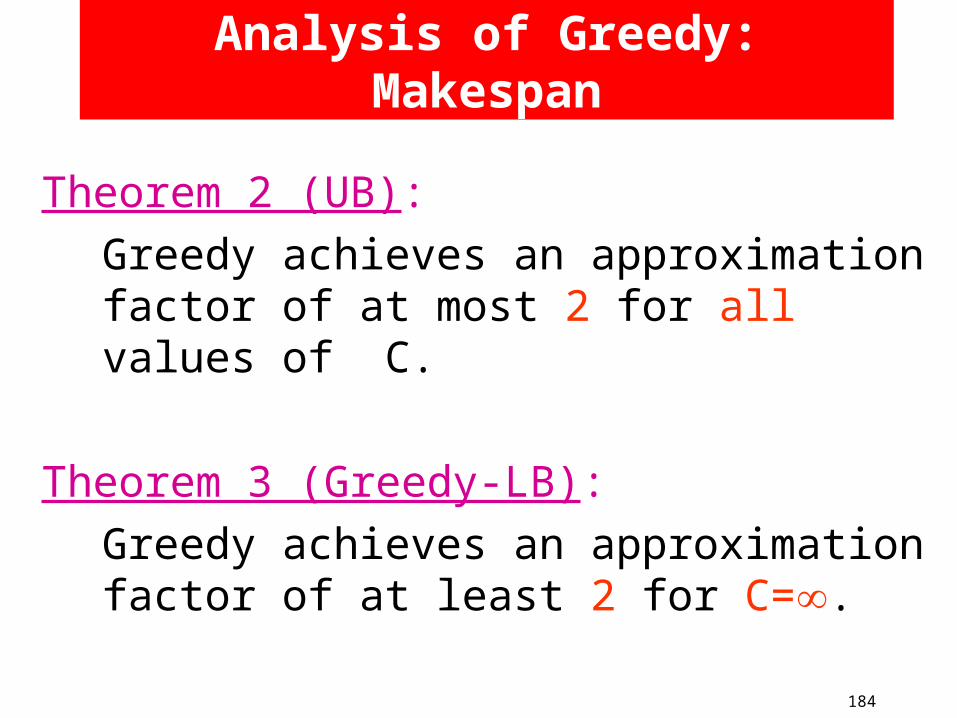
Theorem 2 (UB): Greedy achieves an approximation factor of at most 2 for all values of C.
Theorem 3 (Greedy-LB): Greedy achieves an approximation factor of at least 2 for C=.
Analysis of Greedy: Makespan

185
Consider the k-th matching and let (i,j) be the heaviest edge of weight w.
Lemma 1: There are at least k/2 edges of weight w incident to either input i or output j.
Proof outline: In all iterations 1,...,k-1 Greedy chosen edge of weight w incident to i or j.
Proof of Theorem 2

186
Observation 1: OPT’s schedule contains at least k/2 configurations.
Observation 2: The k/2-th largest holding time in OPT’s schedule is at least w.
The theorem follows !
Proof of Theorem 2 Cont.

187
Theorem 4 (General-LB): The NPBS problem is NP-hard for all values of C and hard to approximate within a factor better than 7/6.
Proof outline: [GW85, CDP01]• Reduction from the Restricted Timetable
Design problem, asg. of teachers for 3 hrs.
• Encoding as a demand matrix, C=.• There is an optimal non-preemptive
schedule that contains 3 matchings.• Works for all values of C !
Hardness Results
188
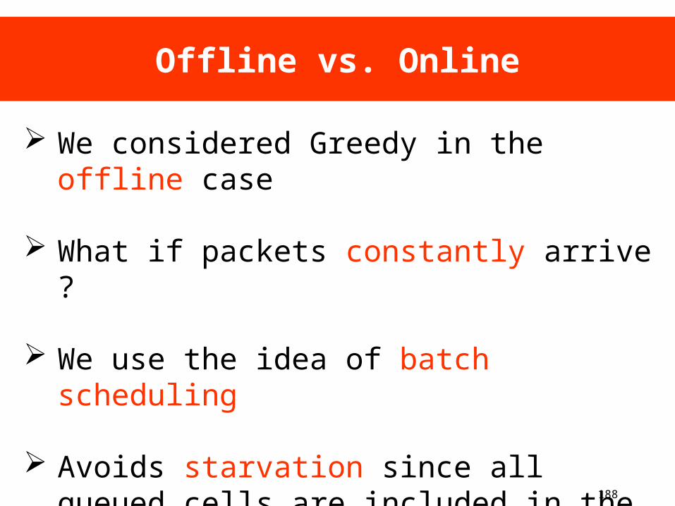
Offline vs. Online
We considered Greedy in the offline case
What if packets constantly arrive ?
We use the idea of batch scheduling
Avoids starvation since all queued cells are included in the next batch

189
Batch Scheduling
N N
1 1R
R
Crossbar
R
R
1
N
1
N
Batch-(k+1)
Batch-(k)
190
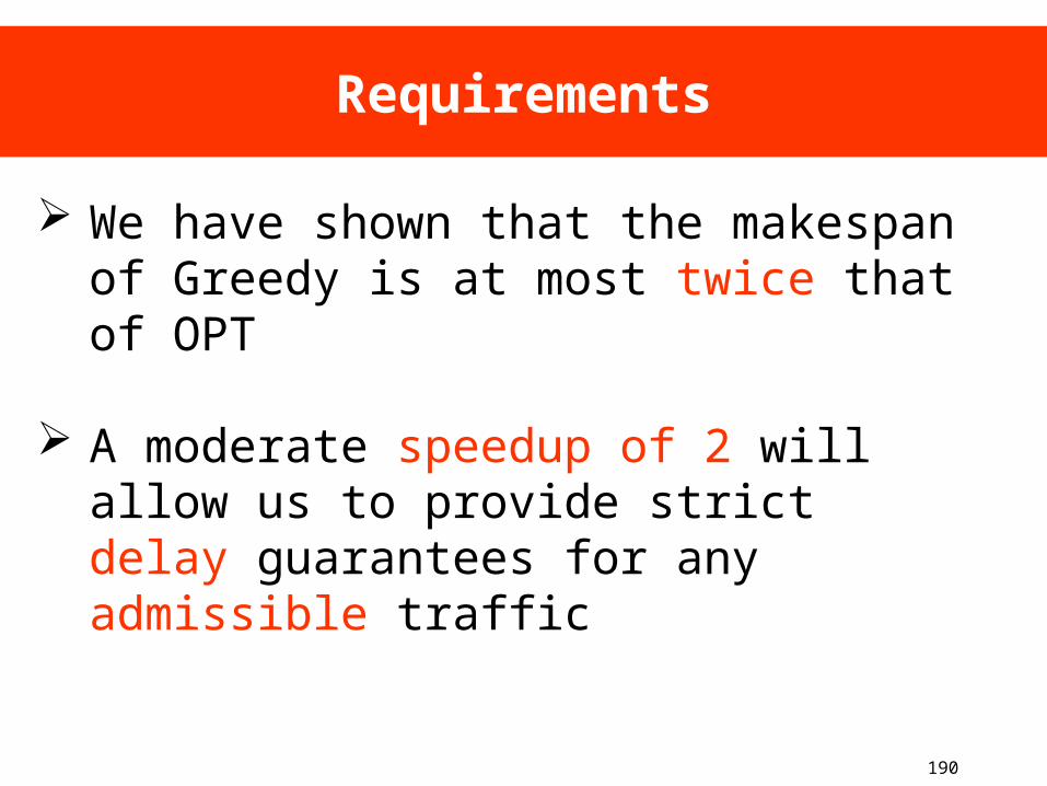
Requirements
We have shown that the makespan of Greedy is at most twice that of OPT
A moderate speedup of 2 will allow us to provide strict delay guarantees for any admissible traffic

191
Open Problems
•Close the gap between the upper and the lower bound (2 vs. 7/6),
•Consider packet-mode scheduling

192
Literature Preemptive scheduling:
[Inukai79] Inukai. An Efcient SS/TDMA Time Slot Assignment Algorithm. IEEE Trans. on Communication, 27:1449-1455, 1979.
[GW85] Gopal and Wong. Minimizing the Number of Switchings in a SS/TDMA System. IEEE Trans. Communication, 33:497-501, 1985.
[BBB87] Bertossi, Bongiovanni and Bonuccelli. Time Slot Assignment in SS/TDMA systems with intersatellite links. IEEE Trans. on Communication, 35:602-608. 1987.
[BGW91] Bonuccelli, Gopal and Wong. Incremental Time Slot Assignement in SS/TDMA satellite systems. IEEE Trans. on Communication, 39:1147-1156. 1991.
[GG92] Ganz and Gao. Efficient Algorithms for SS/TDMA scheduling. IEEE Trans. on Communication, 38:1367-1374. 1992
[CDP01] Crescenzi, Deng and Papadimitriou. On Approximating a Scheduling Problem, Journal of Combinatorial Optimization, 5:287-297, 2001.
[TD02] Towles and Dally. Guaranteed Scheduling for Switches with Conguration Overhead. Proc. of INFOCOM'02.
[LH03] Li and Hamdi, -Adjust Algorithm for Optical Switches with Reconguration Delay. Proc. of ICC'03.
... many others Non-preemptive scheduling:
[PR00] Prais and Ribeiro. Reactive GRASP: An Application to a Matrix Decomposition Problem in TDMA Trafc Assignment. INFORMS Journal on Computing, 12:164-176, 2000.