alabama-coosa-tallapoosa (act) and ... district federal storage reservoir critical yield analyses...

Mobile District

FEDERAL STORAGE RESERVOIR CRITICAL YIELD ANALYSES

ALABAMA-COOSA-TALLAPOOSA (ACT) AND

APALACHICOLA- CHATTAHOOCHEE-FLINT (ACF) RIVER BASINS

February 2010

i

TABLE OF CONTENTS PAGE TITLE NUMBER

EXECUTIVE SUMMARY .................................................................................................1 Scope and Purpose ...................................................................................................1 Critical Yield............................................................................................................2 Methodology............................................................................................................3

Unimpaired Flow Data Set ...............................................................................3 Droughts ...........................................................................................................4 Models ..............................................................................................................4 Method A (Without Diversions).......................................................................5 Method B (With Diversions) ............................................................................6 Method C (River System Yield) .......................................................................6 Assumptions .....................................................................................................7

Critical Yield Analyses Results ...............................................................................8 ACF Basin ........................................................................................................8 ACT Basin ........................................................................................................9

Summary ................................................................................................................10 Acronyms...............................................................................................................11

LIST OF FIGURES FIGURE DESCRIPTION

1 Federal Reservoir Projects in the ACF and ACT Basins.................2 2 Critical Yield Method A (Without Diversions) ...............................5 3 Critical Yield Method B (With Diversions).....................................6 4 Critical Yield Method C (River System Yield) ...............................7

LIST OF TABLES TABLE DESCRIPTION

1 Drought Periods ...............................................................................4 2 Method A, ACF Project Yield (Without Diversions) ......................8 3 Method B, ACF Project Critical Yield (With Diversions) ..............9 4 Method C, ACF (River System Yield) ............................................9 5 Method A, ACT Project Critical Yield (Without Diversions).........9 6 Method B, ACT Project Critical Yield (With Diversions) ............10

ii

Appendix A - Critical Yield Methodology PAGE TITLE NUMBER

1. INTRODUCTION ..................................................................................................... A-1 1.1 Diversions .................................................................................................... A-1

1.1.1 Unimpaired Flow Data Set ................................................................ A-1 1.2 Drought Period Utilized in Critical Yield.................................................... A-2 1.3 Models.......................................................................................................... A-3 1.4 Methods Employed in Critical Yield Analysis ............................................ A-4

1.4.1 Method A (Without Diversions)........................................................ A-5 1.4.2 Method B (With Diversions) ............................................................. A-6 1.4.3 Method C (River System Yield) ........................................................ A-6 1.4.4 Seasonal Storage................................................................................ A-7


A-1 Lake Lanier Pool Elevation 2005-2009...................................... A-3 A-2 Critical Yield Method A (Without Diversions) .......................... A-5 A-3 Critical Yield Method B (With Diversions) ............................... A-6 A-4 Critical Yield Method C (System Critical Yield) ....................... A-7


A-1 Drought Periods .......................................................................... A-2 A-2 Seasonal Conservation Storage Reduction ................................. A-7

iii

Appendix B – Alabama-Coosa-Tallapoosa (ACT) Basin PAGE TITLE NUMBER

1. ACT BASIN................................................................................................................B-1 1.1 Description of Basin .....................................................................................B-1

1.1.1 Climate................................................................................................B-3 1.1.2 Precipitation........................................................................................B-3 1.1.3 Storms and Floods ..............................................................................B-3 1.1.4 Runoff Characteristics ........................................................................B-4

1.2 Reservoirs .....................................................................................................B-7 1.2.1 Reservoir Storage................................................................................B-7 1.2.2 Reservoirs Selected for Yield .............................................................B-8

1.3 Allatoona Dam (Allatoona Lake)..................................................................B-9 1.3.1 Drainage Area.....................................................................................B-9 1.3.2 General Features ...............................................................................B-12

1.3.2.1 Dam ........................................................................................B-12 1.3.2.2 Reservoir.................................................................................B-12

1.3.3 Top of Conservation Pool.................................................................B-14 1.3.4 Regulation Plan.................................................................................B-14 1.3.5 Surface Water Inflows ......................................................................B-15 1.3.6 Unimpaired Flow..............................................................................B-15

1.4 Carters Dam (Carters Lake) ........................................................................B-23 1.4.1 Drainage Area...................................................................................B-23 1.4.2 General Features ...............................................................................B-24

1.4.2.1 Main Dam...............................................................................B-24 1.4.2.2 Reservoir.................................................................................B-26

1.4.3 Top of Conservation Pool.................................................................B-27 1.4.4 Regulation Plan.................................................................................B-28 1.4.5 Surface Water Inflows ......................................................................B-28 1.4.6 Unimpaired Flow..............................................................................B-28

1.5 ResSim Modeling........................................................................................B-36 1.6 Results.........................................................................................................B-37


B-1 ACT Basin ...................................................................................B-1 B-2 Basin Rainfall and Runoff above Rome, Georgia .......................B-5 B-3 Basin Rainfall and Runoff between Claiborne, Alabama and Rome, Georgia ..................................................................B-6 B-4 ACT Basin Reservoir Conservation Storage Percent by Acre-Feet............................................................................B-8

iv

LIST OF FIGURES (Cont’d) PAGE FIGURE DESCRIPTION NUMBER

B-5 Allatoona Dam.............................................................................B-9 B-6 Allatoona Basin Map .................................................................B-10 B-7 Drainage Areas for Projects on the ACT ...................................B-11 B-8 Allatoona Area – Capacity Curves ............................................B-12 B-9 Top and Bottom of Allatoona Conservation Pool......................B-14 B-10 Allatoona Inflow-Outflow-Pool Elevation (Jan 51 – Dec 2009) ................................................................B-16 B-11 Allatoona Unimpaired Annual Inflow Jan 1939 – Dec 2008 .....B-17 B-12 Allatoona Unimpaired Inflow - 1939 – 1943 Drought; 75th Percentile, Average and 25th Percentile Flow...................B-18 B-13 Allatoona Unimpaired Inflow - 1954–1958 Drought; 75th Percentile, Average and 25th Percentile Flow...................B-19 B-14 Allatoona Unimpaired Inflow - 1984–1989 Drought; 75th Percentile, Average and 25th Percentile Flow...................B-20 B-15 Allatoona Unimpaired Inflow - 1998–2003 Drought; 75th Percentile, Average and 25th Percentile Flow...................B-21 B-16 Allatoona Unimpaired Inflow - 2006–2008 Drought; 75th Percentile, Average and 25th Percentile Flow...................B-22 B-17 Carters Dam and Reregulation Dam...........................................B-23 B-18 Carters Basin Map.......................................................................B-24 B-19 Drainage Areas For Projects on the ACT ..................................B-25 B-20 Carters Area – Capacity Curves.................................................B-26 B-21 Top and Bottom of Carters Conservation Pool..........................B-28 B-22 Carters Inflow-Outflow-Pool Elevation (Jul 1975 – Dec 2009).............................................................B-29 B-23 Carters Unimpaired Annual Inflow Jan 1939 – Dec 2008..........B-30 B-24 Carters Unimpaired Inflow – 1940’s Drought; 75th Percentile, Average and 25th Percentile Flow...................B-31 B-25 Carters Unimpaired Inflow – 1950’s Drought; 75th Percentile, Average and 25th Percentile Flow...................B-32 B-26 Carters Unimpaired Inflow – 1980’s Drought; 75th Percentile, Average and 25th Percentile Flow...................B-33 B-27 Carters Unimpaired Inflow - 2000 Drought; 75th Percentile, Average and 25th Percentile Flow...................B-34 B-28 Carters Unimpaired Inflow - 2007 Drought; 75th Percentile, Average and 25th Percentile Flow...................B-35 B-29 ACT ResSim Model Schematic ..................................................B-36 B-30 Allatoona Critical Yield Result, Method A (No Diversions) .....B-38 B-31 Carters Critical Yield Result, Method A (No Diversions)..........B-39 B-32 Allatoona Critical Yield Result, Method A (With Diversions) ..B-40 B-33 Carters Critical Yield Result, Method B (With Diversions).......B-41

v

LIST OF TABLES PAGE TABLE DESCRIPTION NUMBER

B-1 Average Monthly Runoff at Rome, Georgia................................B-5 B-2 Average Monthly Runoff at Claiborne, Alabama........................B-6 B-3 ACT Basin Conservation Storage Percent by Acre-Feet .............B-7 B-4 Lake Allatoona Area and Capacity ............................................B-13 B-5 Carters Reservoir Area and Capacity.........................................B-27 B-6 ACT Project Yield Analysis without River Diversions, Method A ..............................................................................B-38 B-7 ACT Yield Drawdown Period ...................................................B-39 B-8 ACT Projects Yield Analysis with River Diversions, Method B ..............................................................................B-40

vi

Appendix C – Apalachicola-Chattahoochee-Flint (ACF) Basin Detailed Analysis

PAGE TITLE NUMBER

1. ACF BASIN................................................................................................................C-1 1.1 Description of Basin .....................................................................................C-1

1.1.1 Physical Description ...........................................................................C-2 1.1.2 Climate................................................................................................C-3 1.1.3 Precipitation........................................................................................C-3 1.1.4 Storms and Floods ..............................................................................C-4 1.1.5 Runoff Characteristics ........................................................................C-4

1.2 Reservoirs .....................................................................................................C-8 1.2.1 Reservoir Storage................................................................................C-8 1.2.2 Reservoirs Selected for Yield .............................................................C-9

1.3 Buford Dam (Lake Sidney Lanier) ...............................................................C-9 1.3.1 Drainage Area.....................................................................................C-9 1.3.2 Features.............................................................................................C-11

1.3.2.1 Dam ........................................................................................C-12 1.3.2.2 Reservoir.................................................................................C-12

1.3.3 Top of Conservation Pool.................................................................C-14 1.3.4 Regulation Plan.................................................................................C-14 1.3.5 Surface Water Inflows ......................................................................C-15 1.3.6 Unimpaired Flow..............................................................................C-15

1.4 West Point Dam (West Point Lake)............................................................C-23 1.4.1 Drainage Area...................................................................................C-23 1.4.2 Features.............................................................................................C-26

1.4.2.1 Non-Overflow Section............................................................C-26 1.4.2.2 Spillway Section.....................................................................C-26 1.4.2.3 Powerhouse and Intake...........................................................C-26 1.4.2.4 Reservoir.................................................................................C-26


1.5 Walter F. George Dam (Lake Eufaula).......................................................C-38 1.5.1 Drainage Area...................................................................................C-38 1.5.2 General Features ...............................................................................C-41

1.5.2.1 Dam ........................................................................................C-41 1.5.2.2 Reservoir.................................................................................C-41


1.6 ResSim Modeling........................................................................................C-52 1.7 Results.........................................................................................................C-54

vii

LIST OF FIGURES PAGE FIGURE DESCRIPTION NUMBER

C-1 ACF Basin....................................................................................C-1 C-2 Basin Rainfall and Runoff above Atlanta, Georgia .....................C-5 C-3 Basin Rainfall and Runoff between Columbus and Atlanta, Georgia.....................................................................................C-6 C-4 Basin Rainfall and Runoff between Blountstown, FL and Columbus, GA .........................................................................C-7 C-5 ACF Basin Federal Reservoir Conservation Storage Percent By Acre-Feet..........................................................................C-8 C-6 Buford Dam .................................................................................C-9 C-7 Buford Basin Map......................................................................C-10 C-8 Incremental Drainage Basin Map for Federal Projects on the ACF..................................................................................C-11 C-9 Buford Area – Capacity Curves.................................................C-12 C-10 Top and Bottom of Buford Conservation Pool ..........................C-14 C-11 Buford Inflow-Outflow-Pool Elevation (Jul 1957-Dec 2009)...C-16 C-12 Buford Unimpaired Annual Inflow Jan 1939 – Dec 2008.........C-17 C-13 Buford Unimpaired Inflow – 1940’s Drought ...........................C-18 C-14 Buford Unimpaired Inflow – 1950’s Drought ...........................C-19 C-15 Buford Unimpaired Inflow – 1980’s Drought ...........................C-20 C-16 Buford Unimpaired Inflow – 2000 Drought ..............................C-21 C-17 Buford Unimpaired Inflow – 2007 Drought ..............................C-22 C-18 West Point Dam .........................................................................C-23 C-19 West Point Basin Map ...............................................................C-24 C-20 Incremental Drainage Basin Map for Federal Projects on the ACF.................................................................................C-25 C-21 West Point Area – Capacity Curves...........................................C-28 C-22 Top and Bottom of West Point Conservation Pool....................C-29 C-23 West Point Inflow-Outflow-Pool Elevation (Jan 1975-Dec 2009)............................................................C-31 C-24 West Point Unimpaired Annual Inflow Jan 1939 to Dec 2008 .C-32 C-25 West Point Unimpaired Inflow – 1940’s Drought; 75th Percentile, Average and 25th Percentile Flow................C-33 C-26 West Point Unimpaired Inflow – 1950’s Drought; 75th Percentile, Average and 25th Percentile Flow................C-34 C-27 West Point Unimpaired Inflow – 1980’s Drought; 75th Percentile, Average and 25th Percentile Flow................C-35 C-28 West Point Unimpaired Inflow – 2000 Drought; 75th Percentile, Average and 25th Percentile Flow................C-36 C-29 West Point Unimpaired Inflow – 2007 Drought; 75th Percentile, Average and 25th Percentile Flow................C-37 C-30 Walter F. George Dam..............................................................C-38 C-31 Walter F. George Basin Map ....................................................C-39

viii

LIST OF FIGURES (Cont’d) PAGE FIGURE DESCRIPTION NUMBER

C-32 Incremental Drainage Basin Map for Federal Projects on the ACF.................................................................................C-40 C-33 Walter F. George Area - Capacity Curves ................................C-41 C-34 Top and Bottom of Walter F. George Conservation Pool ........C-43 C-35 Walter F. George Inflow-Outflow-Pool Elevation (Jan 1964-Dec 2009)............................................................C-45 C-36 Walter F. George Unimpaired Annual Inflow Jan 1939 to Dec 2008............................................................C-46 C-37 Walter F. George Unimpaired Inflow – 1940’s Drought; 75th Percentile, Average and 25th Percentile Flow................C-47 C-38 Walter F. George Unimpaired Inflow – 1950’s Drought; 75th Percentile, Average and 25th Percentile Flow................C-48 C-39 Walter F. George Unimpaired Inflow – 1980’s Drought; 75th Percentile, Average and 25th Percentile Flow................C-49 C-40 Walter F. George Unimpaired Inflow – 2000 Drought; 75th Percentile, Average and 25th Percentile Flow................C-50 C-41 Walter F. George Unimpaired Inflow – 2007 Drought; 75th Percentile, Average and 25th Percentile Flow................C-51 C-42 ACF ResSim Model Schematic .................................................C-52 C-43 Buford Critical Yield Result, Method A (No Diversions).........C-54 C-44 West Point Critical Yield Result, Method A (No Diversions)...C-55 C-45 Walter F. George Critical Yield Result, Method A (No Diversions).....................................................................C-55 C-46 Buford Critical Yield Result, Method B (With Diversions) ......C-57 C-47 West Point Critical Yield Result, Method B (With Diversions)..................................................................C-57 C-48 Walter F. George Critical Yield Result, Method B (With Diversions)..................................................................C-58 C-49 System Critical Yield Result, Method C (No Diversions).........C-59 C-50 System Critical Yield Result, Method C (With Diversions)......C-60


C-1 Basin Rainfall and Runoff above Atlanta ....................................C-5 C-2 Basin Rainfall and Runoff between Columbus Atlanta...............C-6 C-3 Basin Rainfall and Runoff between Blountstown, FL and Columbus, GA .........................................................................C-7 C-4 ACF Basin Conservation Storage by Project...............................C-8 C-5 Buford Reservoir Area and Capacity Data ................................C-13 C-6 West Point Reservoir Area and Capacity...................................C-27

ix

LIST OF TABLES (Cont’d) PAGE TABLE DESCRIPTION NUMBER

C-7 Walter F. George Reservoir Area and Capacity ........................C-42 C-8 ACF Yield Drawdown Period....................................................C-53 C-9 ACF Yield Analysis Without River Diversions, Method A ......C-54 C-10 ACF Yield Drawdown Period....................................................C-56 C-11 ACF Projects Yield Analysis With River Diversions, Method B ..............................................................................C-56 C-12 ACF System Yield Analysis, Method C....................................C-58

Appendix D – Prior Reports and References TITLE

1. PRIOR REPORTS AND REFERENCES ................................................................. D-1


D-1 Prior Reports................................................................................ D-1

Appendix E – Drought Description TITLE NUMBER

1. DROUGHT DESCRIPTIONS....................................................................................E-1 1.1 2006 - 2008 ...................................................................................................E-1 1.2 1998 – 2003...................................................................................................E-1 1.3 1984 – 1989...................................................................................................E-1 1.4 1954 – 1958...................................................................................................E-1 1.5 1939 – 1943...................................................................................................E-1

1

FEDERAL STORAGE RESERVOIR CRITICAL YIELD ANALYSES

EXECUTIVE SUMMARY

Alabama-Coosa-Tallapoosa and

Apalachicola-Chattahoochee-Flint River Basins

SCOPE AND PURPOSE

The Federal Storage Reservoir Critical Yield Analyses, Alabama-Coosa-Tallapoosa and Apalachicola-Chattahoochee-Flint Basins (Critical Yield Report) provides information and technical analysis in response to Congressional direction in reports accompanying the Energy and Water Development and Related Agencies Appropriations Act, 2010 (H.R. 3183; Public Law 111-85) which includes the following language: “Alabama-Coosa-Tallapoosa [ACT], Apalachicola-Chattahoochee- Flint [ACF] Rivers, Alabama, Florida, and Georgia.—The Secretary of the Army, acting through the Chief of Engineers, is directed to provide an updated calculation of the critical yield of all Federal projects in the ACF River Basin and an updated calculation of the critical yield of all Federal projects in the ACT River Basin within 120 days of enactment of this Act.” Pursuant to this language, the U.S. Army Corps of Engineers (Corps), Mobile District, developed updated critical yields for the Federal projects in the ACF and ACT Basins. Federal reservoirs in the ACF Basin that are included in these analyses are Buford Dam, West Point Dam, and Walter F. George Lock and Dam (reference Figure 1), because they hold the majority of water storage on the ACF System. George Andrews Lock and Dam and Jim Woodruff Lock and Dam are Federal projects on the ACF System that are excluded from the critical yield analyses. These projects are excluded from the analyses because they are ‘run of river’ impoundments with little or no usable water storage, and cannot significantly contribute to critical yield. Federal reservoirs in the ACT River Basin that are included in these analyses are Carters Dam and Allatoona Dam (reference Figure 1), because they hold the majority of water storage in the Federal projects on the ACT System. The Carters Dam System consists of two dams: the main dam and a small, downstream dam impounding discharges from the main dam for pump back purposes. Only the main dam is included in the critical yield evaluations. R.F. Henry Lock and Dam, Millers Ferry Lock and Dam and Claiborne Lock and Dam are Federal reservoirs on the ACT System that are excluded from the critical yield analyses. These reservoirs are excluded from the analyses because they are ‘run of river’ impoundments with little or no usable water storage and cannot significantly contribute to critical yield.

2

Detailed critical yield analyses for the ACF and ACT Basins are presented in separate appendices.

Figure 1. Federal Reservoir Projects in the ACF and ACT Basins

CRITICAL YIELD

Critical yield is the maximum amount of water that can be consistently removed from a reservoir through releases from the dam and/or withdrawals from the reservoir during the most severe drought in the period of record (1939-2008), without depleting the reservoir conservation

3

storage. Conservation storage is the amount of water available in a reservoir to meet project purposes other than flood control. Critical yield is the amount of water available from a reservoir at any time under any conditions described in the hydrologic period of record. The Corps cannot guarantee critical yield will always be available because future droughts may be worse than droughts of the period of record, requiring more conservative operation of reservoirs. Critical yield is important because it is the basis from which water stored in a reservoir is allocated to various project purposes. The amount or volume of water stored in a reservoir can be allocated to a specific project purpose, such as hydropower or water supply, based on a percent of critical yield. A change in critical yield could result in modifications of the allocations for a project purpose. Critical yield can be expressed in cubic feet of water per second (cfs), representing the rate at which water can be removed. Critical yield can also be expressed in millions of gallons per day (mgd) or acre-feet per year (ac-ft/yr), representing the volume of water that can be removed from a reservoir. The conversions between rate and volume are:

1 cfs = 0.6464 mgd = 722.7 ac-ft/yr The analyses in this critical yield report to Congress expresses critical yield in cfs.

METHODOLOGY

This section briefly describes how the Corps determined critical yield and crucial datasets that significantly affect analyses results. A more detailed description of this process is provided in Appendix A - Critical Yield Methodology.

Unimpaired Flow Data Set

The unimpaired flow data set is historically observed flows, adjusted for some of the human influence within the river basins. Man-made changes in the river basins influence water flow characteristics and are reflected in measured flow records. Determining critical yield requires removing identifiable and quantifiable man-made changes such as municipal and industrial water withdrawals and returns, agricultural water use, and increased evaporation and runoff due to the construction of Federal surface water reservoirs, from the observed flow measurements. These quantities are used to extrapolate diversions. The difference between water withdrawn and water returned is defined as a diversion. Diversions are a net volume or quantity assumed to be permanently lost from the water system. The unimpaired flow dataset is not a perfectly replicated flow dataset representing conditions that would exist without the influence of human activities or a precise measure of natural flow conditions. This is because all human influences, such as land use changes, cannot be accounted for, and many flow set adjustments are estimates based upon assumptions, not direct measurements of the human influences.

4

The original unimpaired flow data set developed as part of the Alabama-Coosa-Tallapoosa and Apalachicola Chattahoochee Flint (ACT/ACF) River Basins Comprehensive Water Resources Study, ACT/ACF Comprehensive Water Resources Study, Surface Water Availability Volume I: Unimpaired Flow, July 8, 1997 included data at over 50 locations for the 1939 to 1993 period of record. This data set has recently been extended through 2008 and is available from the Corps. Because of the occurrence of negative flows in the daily values, the data has been smoothed using 3-, 5-, or 7-day averaging. This preserves the volume of the flow and eliminates most of the small negative flows in some of the daily flow data.

Droughts

Several drought periods have been identified from the historic record and from previous yield analyses (reference Appendix D – Prior Reports and References). Drought periods were identified in 1940-41; 1954-58; 1984-89; 1999-2003, and 2006-2008. These are shown below in Table 1. Each period is referenced in accordance to the decade or most severe year of occurrence. Critical yield was computed for each of the drought periods and the lowest value selected as the critical yield value for this report.

Table 1. Drought Periods Drought Periods Label

1940-1941 1940 1954-1958 1950 1984-1989 1980 1999-2003 2000 2006-2008 2007

Models

A computer simulation model is a computer program that simulates a simplified model of a system. The U.S. Army Corps of Engineers’ Hydrologic Engineering Center’s (HEC) Reservoir System Simulation (HEC-ResSim) is a computer program comprised of a graphical user interface (GUI) and a computational engine to simulate reservoir operations. HEC-ResSim was developed to aid engineers and planners performing water resources studies by representing the behavior of reservoirs and to help reservoir operators plan releases in real-time during day-to-day and emergency operations. The HEC-ResSim model has a Firm Yield subroutine which calculates the largest, consistent release that can be reliably supplied during the flow record. The subroutine works by adjusting an operation rule which represents a reservoir management action. The subroutine computes a model simulation run through the period of record with a suggested release toward yield, then recomputes, interating that release until the largest release that can always be successfully made is found. The ResSim ACT and ACF yield models include a net precipitation-evaporation rate for each reservoir that utilizes evaporation values developed for National Oceanic and Atmospheric Administration (NOAA) Technical Reports, monthly pan evaporation rates and National

5

Weather Service (NWS) reports of rainfall and flow rates. The net evaporation losses, evaporation minus precipitation, were computed in inches at the projects. The NOAA report was used because historic monthly evaporation data is not available at the projects. Historic monthly precipitation data was obtained from the NWS. It is important to be aware that the most severe drought event at one reservoir may not be the most severe drought event at another reservoir in the same river system. For the purposes of computing critical yield on the ACF System, the lowest critical yield value (typically associated with the most severe drought event) at an upstream reservoir will be used to calculate a downstream reservoir’s critical yield. This is because on the ACF System, the amount of water exiting an upstream reservoir influences the amount of water available in a downstream reservoir. This is germane to Methods A and B described below.

Method A (Without Diversions)

Method A assumes that there are no withdrawals from or returns to the lake and there are no withdrawals from or returns to the river as it flows between projects. This condition results in the maximum yield possible from the Federal projects. Critical yield from an upstream reservoir is assumed to be permanently removed from the system and does not contribute to the inflow at downstream reservoirs.

Figure 2. Critical Yield Method A (Without Diversions)

6

Method B (With Diversions)

Method B assumes net river withdrawals and returns are occurring; this method does not include withdrawals from the Corps reservoirs. Critical yield from an upstream reservoir is assumed to be permanently diverted from the system and does not contribute to the inflow at downstream reservoirs. This condition results in the most severe downstream impact. The results of Method B represent a conservative assessment of the critical yield available from Federal projects controlled by the Corps of Engineers. Method B used the most severe drought events documented during the hydrologic period of record and the year of maximum river withdrawals (2006 for the ACT; 2007 for the ACF) to make the calculations.

Figure 3. Critical Yield Method B (With Diversions)

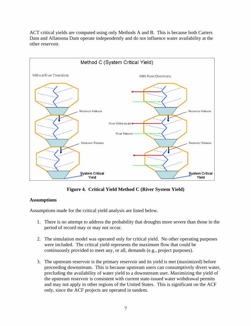
Method C (River System Yield)

Method C computes a system yield for diversion from the most downstream storage reservoir. It assumes upstream reservoirs operate in tandem to maximize the critical yield at the most downstream reservoir. Method C computes critical yield for the ACF River System with and without net river withdrawals. The with net river withdrawals condition results represent the Corps’ yield. The without net river withdrawals condition results represent the system theoretical maximum yield. Method C calculates the theoretical critical yield that might be observed if the upstream projects were operated solely to maximize yield at Walter F. George Lake. However, in reality the results could not be achieved because the Corps must operate in a balanced manner to achieve all authorized project purposes.

7

ACT critical yields are computed using only Methods A and B. This is because both Carters Dam and Allatoona Dam operate independently and do not influence water availability at the other reservoir.

Figure 4. Critical Yield Method C (River System Yield)

Assumptions

Assumptions made for the critical yield analysis are listed below.

1. There is no attempt to address the probability that droughts more severe than those in the period of record may or may not occur.

2. The simulation model was operated only for critical yield. No other operating purposes

were included. The critical yield represents the maximum flow that could be continuously provided to meet any, or all, demands (e.g., project purposes).

3. The upstream reservoir is the primary reservoir and its yield is met (maximized) before

proceeding downstream. This is because upstream users can consumptively divert water, precluding the availability of water yield to a downstream user. Maximizing the yield of the upstream reservoir is consistent with current state-issued water withdrawal permits and may not apply in other regions of the United States. This is significant on the ACF only, since the ACF projects are operated in tandem.

8

4. Yield analysis is based on currently authorized conservation storage elevations.

5. Projects are full at the beginning of the drought period simulation. The pool level at the beginning of a drought simulation is important because it is a variable that directly affects the quantity or volume of water available as critical yield.

6. None of the critical yield is returned to the system. Critical yield is permanently diverted

from the system and assumed to be consumptively used. For example: Buford Dam critical yield is not counted as inflow to West Point Lake. Inflows to West Point Lake are assumed to derive only from the West Point Lake drainage basin. This methodology determines the conservative individual project yield. The assumption is applicable to Methods A and B. The assumption is not applicable to Method C.

7. Existing area capacity curves as shown in the latest water control manuals were used.

CRITICAL YIELD ANALYSES RESULTS

A summary of model results is presented below for each basin. A more detailed description of basin-specific methods, modeling and results is presented in the Appendix B - ACT Basin and Appendix C - ACF Basin.

ACF Basin

Tables 2 and 3 list the critical yield of each federal reservoir on the ACF System and the critical drought period used in the calculations.

Table 2. Method A, ACF Project Yield (Without Diversions)

Project Critical Yield (cfs) Critical Drought

Buford Dam 1,465 1980

West Point Dam 1,167 2007

Walter F. George Lock and Dam 572 2007

The ACF River System diversions are municipal, industrial and agricultural withdrawals and returns from the Chattahoochee River and its tributaries located upstream of Lake Sidney Lanier, West Point Lake and Walter F. George Lake. Maximum river withdrawals occurred in 2007 and are reflected in the critical yield calculation for each drought period. Computation of Method A, ACF Project Yield (Without Diversions) did not include these withdrawals.

9

Table 3. Method B, ACF Project Critical Yield (With Diversions)

Project

Critical Yield (cfs)

Critical Drought

Critical Yield Reduction

Attributable To Diversions Buford Dam 1,460 1980's 0.4% West Point Dam 891 2007 24% Walter F. George Lock and Dam 470 2007 18%

Comparing the critical yield results from the Method A (Without Diversions) and Method B (With Diversions) allows us to quantify the impacts of the river withdrawals. The 2007 river withdrawals had a measurable impact, reducing critical yield as much as 23 percent at West Point and 17 percent at Walter F. George. Table 4 below lists the Method C (River System Yield) results of operating the three ACF reservoirs together for a system yield at Walter F. George. When all reservoirs are operated for yield optimization at Walter F. George, the system yield obtained is greater than the sum of the individual reservoir yields. Method C (River System Yield) was computed with and without river diversions. The 2007 river diversions reduce the critical yield at Walter F. George by 16 percent. This figure represents the percentage difference between 4,370 cfs (ACF System Without Divisions) and 3,683 cfs (ACF System With Diversions).

Table 4. Method C, ACF (River System Yield)

Project System Critical Yield

(cfs) Critical Drought

ACF System (Without Diversions) 4,370 2007

ACF System (With Diversions) 3,683 2007

ACT Basin

Tables 5 and 6 list the critical yield of each project and the critical drought period used in the calculations.

Table 5. Method A, ACT Project Critical Yield (Without Diversions) Project Critical Yield (cfs) Critical Drought

Allatoona Dam 729 2007 Carters Dam 390 2007

The ACT River System diversions are municipal, industrial and agricultural withdrawals and returns from the Coosawattee River and it tributaries upstream of Carters Lake and from the Etowah River and its tributaries upstream of Allatoona Lake. Maximum diversions occurred in 2006 and are reflected in the critical yield calculation for each drought period.

10

Table 6. Method B, ACT Project Critical Yield (With Diversions)

Project Critical Yield (cfs) Critical Drought Critical Yield Reduction

Attributable To Diversions

Allatoona Dam 693 2007 4.9%

Carters Dam 387 2007 0.8%

Comparing the yield results from the Method A (Without Diversions) and Method B (With Diversions) allows us to quantify the impacts of the river withdrawals. The 2006 river diversions have a measurable impact on the critical yield, as much as five percent at Allatoona Lake (reference Table 5).

SUMMARY

The results of Method B (With Diversions) (reference Tables 3 and 6) for both basins represent a realistic assessment of the critical yield from Federal projects controlled by the Corps. Historical critical yield determinations are referenced in Appendix D - Prior Reports and References. The reader should be cautioned that there is not a direct correlation between the finding of historical critical yields and the findings of this Critical Yield Report. This is due to differences in the drought periods used in each set of analyses and methods employed to calculate the critical yield.

11

ACRONYMS Acres ac acre-feet ac-ft acre-feet per year ac-ft/yr Alabama-Coosa-Tallapoosa ACT Apalachicola-Chattahoochee-Flint ACF cubic feet per second cfs elevation Elev Federal Energy Regulatory Commission FERC graphical user interface GUI Hydrologic Engineer Center HEC Hydrologic Engineering Center’s, Reservoir Simulation Model HEC-ResSim Kilowatt kW Million gallons per day mgd Mean Sea Level msl Megawatt MW National Geodetic Vertical Datum of 1929 NGVD 29 National Oceanic and Atmospheric Administration NOAA National Weather Service NWS Revised Interim Operating Plan RIOP U.S. Army Corps of Engineers Corps United States Geological Survey USGS

Appendix A

Critical Yield Methodology

A-1

Appendix A - Critical Yield Methodology

1 INTRODUCTION The methodology describing how the Corps determined critical yield and crucial datasets that significantly affect analyses results is detailed below.

1.1 RIVER DIVERSIONS

The difference between water withdrawn from a river and water returned to the river is defined as a diversion. Diversions are a net volume or quantity assumed to be permanently lost from the river.

1.1.1 Unimpaired Flow Data Set

The unimpaired flow data set is historically observed flows, adjusted for some of the human influence within the river basins. Man-made changes in the river basins influence water flow characteristics and are reflected in measured flow records. Determining critical yield requires removing identifiable and quantifiable man-made changes such as municipal and industrial water withdrawals and returns, agricultural water use, and increased evaporation and runoff due to the presence of surface water reservoirs, from the observed flow measurements. The daily unimpaired flow data set is used as the input flow series for all yield model simulations and represents the Corps’ best estimate of a pre-development flow series. By making these flow adjustments for man-made activities, any combination of water demands input to the ResSim model and modeled over the entire flow record (1939 – 2008), produces a consistent basis for comparing yield results. Yield simulations are computed for with no water diversion and with current water diversion scenarios using current river diversions to compute yield accounts for existing conditions. The unimpaired flow dataset is not an exact replication of a flow dataset representing conditions that would exist without the influence of human activities or a precise measure of natural flow conditions. This is because all human influences, such as land use changes, cannot be accounted for, and many flow set adjustments are estimates based upon assumptions, not direct measurements of the human influences. The original unimpaired flow data set developed as part of the Alabama-Coosa-Tallapoosa and Apalachicola Chattahoochee Flint (ACT/ACF) River Basins Comprehensive Water Resources Study, ACT/ACF Comprehensive Water Resources Study, Surface Water Availability Volume I: Unimpaired Flow, July 8, 1997 . The Comprehensive Study was study conducted by the States of Alabama, Florida and Georgia and the Corps pursuant to a Memorandum of Understanding. One purpose of the study was to identify available water resources and water demands in the ACT and ACF Basins, and recommend a coordination mechanism for the equitable allocation of water resources between the States. Several technical modeling and assessment tools were developed to support this process, including the unimpaired flow dataset and the HEC-5 hydrological model.

A-2

The process accumulated data at over 50 locations for the 1939 to 1993 period of record. Because of the occurrence of negative flows in the daily values, the data has been smoothed using 3-, 5-, or 7-day averaging. This preserves the volume of the flow and eliminates most of the small negative flows in some of the daily flow data. The Mobile District modeling team develops the unimpaired flow data sets every 1 - 3 years employing water use data provided by the States of Alabama, Florida and Georgia. The unimpaired flow datasets are reviewed by the states before finalizing. All supporting data and the final results of the analyses are provided to the states. This data set has recently been extended through 2008 and is available from the Corps of Engineers.

1.2 DROUGHT PERIOD UTILIZED IN CRITICAL YIELD

Several drought periods have been identified from the historic record and from previous yield analyses (reference Appendix D - References and Prior Reports). Drought periods were identified in 1940-41; 1954-58; 1984-89; 1999-2003, and 2006-2008. These are shown below in Table A-1 and described in more detail at Appendix E - Drought Descriptions. Each period is referenced in accordance to the decade or most severe year of occurrence. Critical yield was computed for each of the drought periods and the lowest value selected as the critical yield value for this report.

Table A-1. Drought Periods

Drought Periods Label

1940-1941 1940

1954-1958 1950

1984-1989 1980

1999-2003 2000

2006-2008 2007

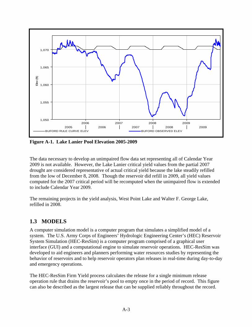
The most recent drought and recovery period extend beyond 2008. Lake Lanier reached a historic low elevation of 1050.79 feet NGVD on December 28, 2007, and nearly again on December 8, 2008, when the pool reached elevation 1051 feet NGVD. A return to almost normal rainfall and conservative management allowed the reservoir to refill 20 feet over the next 10 months. Lake Lanier recovery was marked by reaching full pool elevation of 1071 feet NGVD on October 14, 2009. Figure A-1 shows the most recent critical period for Lake Lanier and includes the drawdown and refill period through 2009.

A-3

Figure A-1. Lake Lanier Pool Elevation 2005-2009 The data necessary to develop an unimpaired flow data set representing all of Calendar Year 2009 is not available. However, the Lake Lanier critical yield values from the partial 2007 drought are considered representative of actual critical yield because the lake steadily refilled from the low of December 8, 2008. Though the reservoir did refill in 2009, all yield values computed for the 2007 critical period will be recomputed when the unimpaired flow is extended to include Calendar Year 2009. The remaining projects in the yield analysis, West Point Lake and Walter F. George Lake, refilled in 2008.

1.3 MODELS

A computer simulation model is a computer program that simulates a simplified model of a system. The U.S. Army Corps of Engineers’ Hydrologic Engineering Center’s (HEC) Reservoir System Simulation (HEC-ResSim) is a computer program comprised of a graphical user interface (GUI) and a computational engine to simulate reservoir operations. HEC-ResSim was developed to aid engineers and planners performing water resources studies by representing the behavior of reservoirs and to help reservoir operators plan releases in real-time during day-to-day and emergency operations. The HEC-ResSim Firm Yield process calculates the release for a single minimum release operation rule that drains the reservoir’s pool to empty once in the period of record. This figure can also be described as the largest release that can be supplied reliably throughout the record.

2006 2007 2008 2009

2005 2006 2007 2008 2009

Ele

v (ft)

1,050

1,055

1,060

1,065

1,070

BUFORD RULE CURVE ELEV BUFORD OBSERVED ELEV

A-4

The process involves computing a simulation run with an estimate of the largest release, and recomputing iteratively with successive estimates until the correct release is found. The user enters the maximum number of iterations that will be run and two tolerance values. The Storage Test Tolerance value shares the same units as the reservoir storage and is the value the reservoir must decrease in order to be considered empty. It will be used as the tolerance for all the zone storage values listed in the reservoir table. The Rule Test Tolerance value will share the same units as the minimum release rule and is used in the calculations as a test for violations of the minimum release rule. The ResSim ACT and ACF yield models include a net precipitation-evaporation rate for each reservoir that utilizes evaporation values developed for National Oceanic and Atmospheric Administration (NOAA) Technical Reports, monthly pan evaporation rates and National Weather Service (NWS) reports of rainfall and flow rates. The net evaporation losses, evaporation minus precipitation, were computed in inches at the projects. The NOAA report was used because historic monthly evaporation data is not available at the projects. Historic monthly precipitation data was obtained from the NWS.

1.4 METHODS EMPLOYED IN CRITICAL YIELD ANALYSIS

There are several ways of computing critical yield. Sequential analysis is currently the most accepted method. This method uses the conservation of mass principles to account for the water in the reservoir inflows and releases. The fundamental equation is:

I - O = ∆ S Where: I = Total inflow during the time period, in volume units O = Total outflow during the time period, in volume units ∆ S = Change in storage during the time period, in volume units Sequential routing uses an iterative form of the above equation:

St = St-1 + It - Ot Where: St = Storage at the end of time t, volume units St-1 = Storage at the end of time t-1, volume units It = Average inflow during time step ∆, in volume units Ot = Average outflow during time step ∆, in volume units

A-5

The HEC-ResSim computer application uses sequential analysis and the sequential routing method with the application’s Firm Yield routine to maximize yield from a specified amount of storage. It is important to be aware that the most severe drought event at one reservoir may not be the most severe drought event at another reservoir in the same river system. For the purposes of computing critical yield on the ACF System, the lowest critical yield value (typically associated with the most severe drought event) at an upstream reservoir will be used to calculate a downstream reservoir’s critical yield. This is because on the ACF System, the amount of water exiting an upstream reservoir influences the amount of water available in a downstream reservoir. This is germane to Methods A and B described below.

1.4.1 Method A (Without Diversions)

Method A assumes that there are no withdrawals from or returns to the lake or the river as it flows between projects. This condition results in the maximum yield possible from the Federal projects. Critical yield from an upstream reservoir is assumed to be permanently removed from the system and does not contribute to the inflow at downstream reservoirs.

Figure A-2. Critical Yield Method A (Without Diversions)

A-6

1.4.2 Method B (With Diversions)

Method B assumes net river withdrawals and returns are occurring; this method does not include withdrawals from the Corps reservoirs. Critical yield from an upstream reservoir is assumed to be permanently diverted from the system and does not contribute to the inflow at downstream reservoirs. This condition results in the most severe downstream impact. The results of Method B represent a realistic assessment of the critical yield available from Federal projects controlled by the Corps. Method B used the most severe drought events documented during the hydrologic period of record and the year of maximum river withdrawals (2006 for the ACT; 2007 for the ACF) to make the calculations.

Figure A-3. Critical Yield Method B (With Diversions)

1.4.3 Method C (River System Yield)

Method C computes a system yield for diversion from the most downstream storage reservoir. It assumes upstream reservoirs operate in tandem to maximize the critical yield at the most downstream reservoir. Method C computes critical yield for the ACF River System with and without net river withdrawals. The with net river withdrawals condition results represent the Corps’ yield. The without net river withdrawals condition results represent the system theoretical maximum yield.

A-7

ACT critical yields are computed using only Methods A and B. This is because both Carters Dam and Allatoona Dam operate independently and do not influence water availability at the other reservoir.

Figure A-4. Critical Yield Method C (System Critical Yield)

1.4.4 Seasonal Storage

The amount of conservation storage is seasonal at federal projects because of the seasonal drawdown to support flood reduction operations. Table A-2 lists the elevation difference in the guide curve and reduction in conservation storage for the federal projects.

Table A-2. Seasonal Conservation Storage Reduction

Project

Elevation Difference (feet)

Storage Difference (ac-ft)

Percent Reduction In Conservation Storage

Allatoona 17 = 840-823 164,702 58% Carters 2 = 1074-1072 6,492 5% Buford 1 = 1071 – 1070 38,200 4% West Point 7 = 635 – 628 162,232 53% Walter F. George 2 = 190 – 188 87,300 36%

A-8

For Allatoona, West Point and Walter F. George, the yield of these projects is highly dependent on the beginning of the critical dry period. In other words, does it begin during the winter level, summer level or transition level of the guide curve? Although all three projects have a high probability of refill to summer pool from a low winter level, extreme rare events will prevent the project from refilling. Consequently, if the critical period begins before the reservoir reaches full summer level the critical yield will be lower than when compared to starting at full summer level. For the determination of critical yields, the yield simulation begins approximately one year before the drought period begins. The analyses assume about one year of normal flows prior to the beginning of the drought period. Drawdown could start whenever flows were low enough for the lake to fall below a target level, be it winter, summer or transition. For the efficiency of computations, separate drought periods were run, always considering the prior year average flows and assuming the highest possible elevation on the guide curve as the target level.

Appendix B

Alabama-Coosa-Tallapoosa (ACT) Basin

B-1

Appendix B - Alabama-Coosa-Tallapoosa (ACT) Basin

1 ACT BASIN

1.1 DESCRIPTION OF BASIN

The headwater streams of the Alabama-Coosa-Tallapoosa (ACT) System rise in the Blue Ridge Mountains of Georgia and Tennessee and flow southwest, combining at Rome, Georgia, to form the Coosa River. The confluence of the Coosa and Tallapoosa Rivers in central Alabama forms the Alabama River, which flows through Montgomery and Selma and joins with the Tombigbee River at the bottom of the ACT Basin about 45 miles above Mobile to form the Mobile River. The Mobile River flows into Mobile Bay at an estuary of the Gulf of Mexico. The total drainage area of the ACT Basin is approximately 22,800 square miles. Progressing downstream from the headwater are the Cities of Rome, Georgia, Gadsden, and Montgomery, Alabama in the central portion of Alabama. The largest metropolitan area in the basin is Montgomery, Alabama.

Figure B-1. ACT Basin

B-2

Beginning in the headwaters of northeast Georgia with spring fed mountain streams the slope is steep, with rapid runoff during rainstorms. Some of the most upstream tributaries are the Oostanaula River, the Conasauga River, Ellijay River, the Cartecay River and Etowah River. The Etowah River, which joins the Oostanaula River at Rome, Georgia, to form the Coosa River, lies entirely within Georgia. It is formed by several small mountain creeks which rise on the southern slopes of the Blue Ridge Mountains at an elevation of about 3,250 feet. The river flows southerly, southwesterly, and then northwesterly for 150 miles to Rome, Georgia. The drainage basin of 1,860 square miles has a maximum width of about 40 miles and a length of about 70 miles. Allatoona Dam is located on the Etowah River near Cartersville, Georgia. It is a multiple-purpose Corps project placed in operation early in 1950 and provides storage for power and flood control. Principal tributaries of the Etowah River are Amicalola, Settingdown, Shoal, Allatoona, Pumpkinvine and Euharlee Creeks and Little River. Three of these, Allatoona and Shoal Creeks, and Little River drain into Lake Allatoona. The Coosawattee River is 45 miles long; and has a fall of 650 feet, an average of 14.4 feet per mile. The Carters Project is located on the Coosawattee River at river mile 26.8. This federal project consists of an earth-fill dam, and a downstream re-regulation reservoir that accommodates pump-back operations. The Conasauga River, with its tributary Jacks River, rises on the northern slopes of the Cohutta Mountains in Fanning County, Georgia, at an elevation of about 3,150 feet. Its drainage basin, 727 square miles, has a maximum width of 25 miles and a length of 40 miles. The eastern and northern portions of the basin are rugged and mountainous, containing peaks over 4,000 feet in elevation. The river flows 90 miles from the headwater to join the Coosawattee River to form the Oostanaula River. From its source at the confluence of the Coosawattee and Conasauga Rivers at Newtown Ferry, Georgia., the Oostanaula River meanders southwesterly through a broad plateau for 47 miles to its mouth at Rome, Georgia. Its total drainage area is 2,160 square miles. The Coosa River, which is formed by the Etowah and Oostanaula Rivers at Rome, Georgia, flows first westerly, then southwesterly and finally southerly a total distance of 286 miles to its mouth, 11 miles below Wetumpka, Alabama, where it joins the Tallapoosa to form the Alabama River. The drainage area of the Coosa River is approximately 10,200 square miles. Alabama Power Company operates eleven dams with seven on the Coosa River. These are Weiss Dam, H. Neely Henry Dam, Logan Martin Dam, Lay Dam, Mitchell Dam, and Jordan-Bouldin Dams. The Tallapoosa River, with a drainage area of 4,680 square miles, rises in northwestern Georgia at an elevation of about 1,250 feet, and flows westerly and southerly for 268 miles, joining the Coosa River south of Wetumpka, Alabama to form the Alabama River. There are four large power dams owned by the Alabama Power Company on the Tallapoosa River. These are Harris Dam, Martin Dam, Yates Dam, and Thurlow Dam. The Alabama River meanders from the head near Wetumpka through the Coastal Plain westerly for about 100 miles to Selma, Alabama. From there it flows southwesterly 214 miles to its

B-3

mouth near Calvert, Alabama. There are three Corps projects on the Alabama River. Robert F. Henry Lock and Dam and Millers Ferry Lock and Dam provide for hydropower and navigation. Claiborne Lock and Dam provides for navigation only.

1.1.1 Climate

The chief factors that control the climate of the Alabama-Coosa-Tallapoosa Basin are its geographical position in the southern end of the Temperate Zone, its proximity to the Gulf of Mexico and South Atlantic Ocean, and its range in altitude from almost sea level at the southern end to over 4,000 feet in the Blue Ridge Mountains to the north. The proximity of the warm South Atlantic and the semitropical Gulf of Mexico insures a warm, moist climate. Extreme temperatures range from near 110 degrees in the summer to values below zero in the winter. Severe cold weather rarely lasts longer than a few days. The summers, while warm, are usually not oppressive. In the southern end of the basin the average maximum January temperature is 60 degrees and the average minimum January temperature is 37 degrees. The Maximum average July temperature is 91 degrees; in the southern end of the basin the corresponding minimum value is 69 degrees. The frost-free season varies in length from about 200 days in the northern valleys to about 250 days in the southern part of the basin. Precipitation is mostly in the form of rain, but some snow falls in the mountainous northern region on an average of twice a year.

1.1.2 Precipitation

The entire ACT Watershed lies in a region which ordinarily receives an abundance of precipitation. The watershed receives a large amount of rain and it is well distributed throughout the year. Winter and spring are the wettest periods and early fall the driest. Light snow is not unusual in the northern part of the watershed, but constitutes only a very small fraction of the annual precipitation and has little effect on runoff. Intense flood producing storms occur mostly in the winter and spring. They are usually of the frontal-type, formed by the meeting of warm moist air masses from the Gulf of Mexico with the cold, drier masses from the northern regions, and may cause heavy precipitation over large areas. The storms that occur in summer or early fall are usually of the thunderstorm type with high intensities over smaller areas. Tropical disturbances and hurricanes can occur producing high intensities of rainfall over large areas.

1.1.3 Storms and Floods

Major flood-producing storms over the ACT Watershed are usually of the frontal type, occurring in the winter and spring and lasting from 2 to 4 days, with their effect on the basin depending on their magnitude and orientation. The axes of the frontal-type storms generally cut across the long, narrow basin. Frequently a flood in the lower reaches is not accompanied by a flood in the upper reaches and vice versa. Occasionally, a summer storm of the hurricane type, such as the storms of July 1916 and July 1994, will cause major floods over practically the entire basin. However, summer storms are usually of the thunderstorm type with high intensities over small areas producing serious local floods. With normal runoff conditions, from 5 to 6 inches of intense and general rainfall are required to produce wide spread flooding, but on many of the minor tributaries 3 to 4 inches are sufficient to produce local floods.

B-4

Historically, minor or major floods within the ACT Basin occur about two times per year. The storms which occurred in July 1916, December 1919, March 1929, February 1961, and July 1994 are of special interest because of the intensities of precipitation over large areas. It should be noted that they represent both the hurricane and frontal types which produce the great floods in this area.

1.1.4 Runoff Characteristics

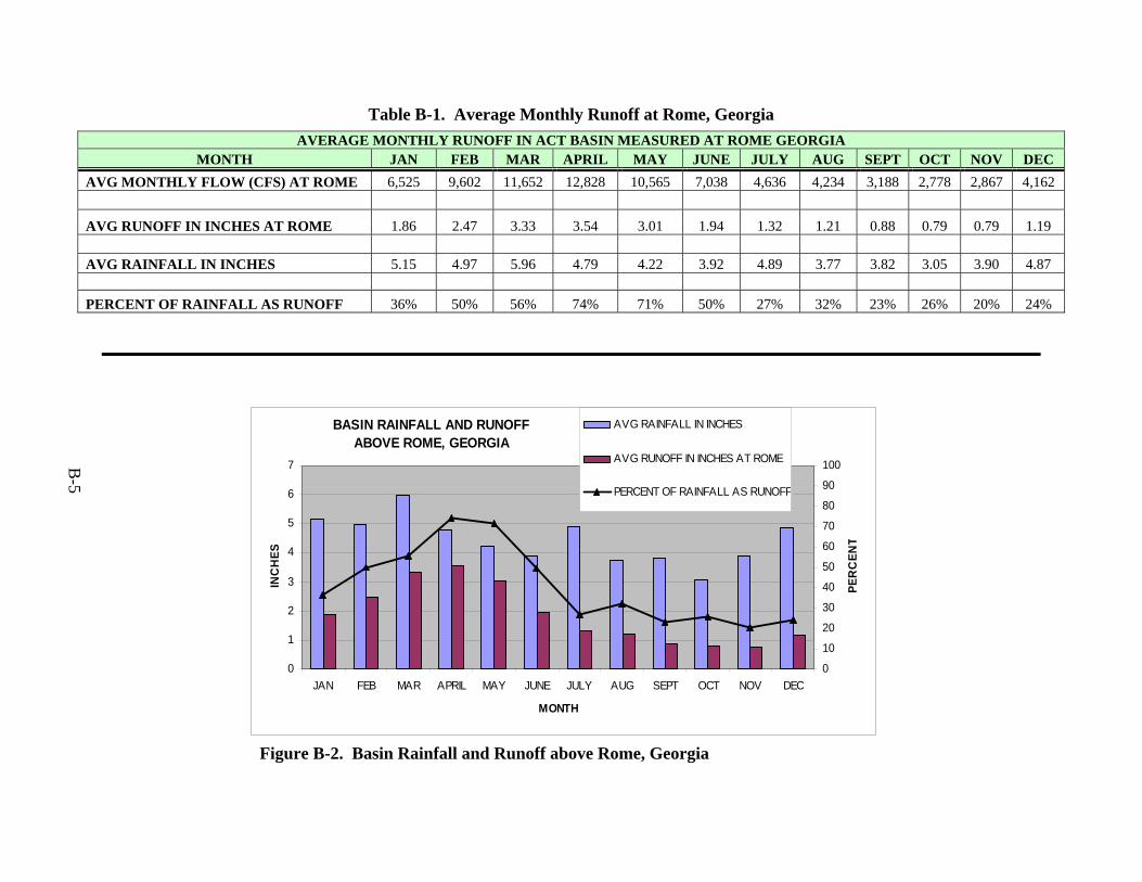
Within the ACT Basin rainfall occurs throughout the year but is less abundant during the August through November time frame. The amount of this rainfall that actually contributes to streamflow varies much more than the rainfall. Several factors such as plant growth and the seasonal rainfall patterns contribute to the volume of runoff. Table B-1 and Table B-2 present the average monthly runoff for the basin. These tables divide the basin at Rome Georgia to show the different percentages of runoff verses rainfall for the northern and southern sections. The mountainous areas exhibit flashier runoff characteristics and somewhat higher percentages of runoff. Figure B-2 and Figure B-3 present the same information in graphical form.

B-5

Table B-1. Average Monthly Runoff at Rome, Georgia

Figure B-2. Basin Rainfall and Runoff above Rome, Georgia

AVERAGE MONTHLY RUNOFF IN ACT BASIN MEASURED AT ROME GEORGIA MONTH JAN FEB MAR APRIL MAY JUNE JULY AUG SEPT OCT NOV DEC

AVG MONTHLY FLOW (CFS) AT ROME 6,525 9,602 11,652 12,828 10,565 7,038 4,636 4,234 3,188 2,778 2,867 4,162

AVG RUNOFF IN INCHES AT ROME 1.86 2.47 3.33 3.54 3.01 1.94 1.32 1.21 0.88 0.79 0.79 1.19 AVG RAINFALL IN INCHES 5.15 4.97 5.96 4.79 4.22 3.92 4.89 3.77 3.82 3.05 3.90 4.87

PERCENT OF RAINFALL AS RUNOFF 36% 50% 56% 74% 71% 50% 27% 32% 23% 26% 20% 24%

BASIN RAINFALL AND RUNOFFABOVE ROME, GEORGIA

0

1

2

3

4

5

6

7

JAN FEB MAR APRIL MAY JUNE JULY AUG SEPT OCT NOV DEC

MONTH

INC

HE

S

0

10

20

30

40

50

60

70

80

90

100

PE

RC

EN

T

AVG RAINFALL IN INCHES

AVG RUNOFF IN INCHES AT ROME

PERCENT OF RAINFALL AS RUNOFF

B-6

Table B-2. Average Monthly Runoff at Claiborne, Alabama

Figure B-3. Basin Rainfall and Runoff between Claiborne, Alabama and Rome, Georgia

AVERAGE MONTHLY RUNOFF IN ACT BASIN MEASURED AT CLAIBORNE ALABAMA MONTH JAN FEB MAR APRIL MAY JUNE JULY AUG SEPT OCT NOV DEC

AVG MONTHLY FLOW (CFS) AT CLAIBORNE 31,529 47,762 58,487 69,862 57,732 32,294 19,981 18,553 14,386 11,346 11,279 16,606 INCREMENTAL FLOW BETWEEN CLAIBORNE AND ROME 25,004 38,160 46,835 57,034 47,167 25,256 15,345 14,319 11,198 8,568 8,412 12,444 AVG RUNOFF IN INCHES BETWEEN CLAIBORNE AND ROME 1.65 2.52 3.10 3.77 3.12 1.67 1.01 0.95 0.74 0.57 0.56 0.82 AVG RAINFALL IN INCHES 5.19 5.15 6.10 4.90 4.18 4.16 5.28 3.95 3.63 2.84 4.07 4.93 PERCENT OF RAINFALL AS RUNOFF 32% 49% 51% 77% 75% 40% 19% 24% 20% 20% 14% 17%

BASIN RAINFALL AND RUNOFFBETWEEN CLAIBORNE AND ROME

0

1

2

3

4

5

6

7


MONTH

INC

HE

S

0

10

20

30

40

50

60

70

80

90

100

PE

RC

EN

T


AVG RUNOFF IN INCHES

PERCENT OF RUNOFF ASRAINFALL

B-7

1.2 RESERVOIRS

1.2.1 Reservoir Storage

Within the Alabama-Coosa-Tallapoosa River Basin there are five (5) federally owned reservoir projects; Carters Dam (Carters Lake ), Allatoona Dam (Allatoona Lake), R.F. Henry Lock and Dam (Jones Bluff Powerhouse and Woodruff Reservoir), Millers Ferry Lock and Dam (William Danelly Lake), and Claiborne Lock and Dam (Claiborne Lake). These projects were built and are operated by the Corps, Mobile District Office. The Alabama Power Company owns and operates seven dams on the Coosa River and four on the Tallapoosa River. The reservoir storage in the basin controlled by each of the reservoirs is listed in Table B-3 and shown graphically in Figure B-4. Claiborne Lock and Dam is not shown because the storage is insignificant.

Table B-3. ACT Basin Conservation Storage Percent by Acre-Feet

Project

Conservation Storage (ac-ft)

Percentage

*Allatoona 284,589 12%

*Carters 141,400 6%

Weiss 237,448 10%

Neely Henry 43,205 2%

L Martin 108,262 4%

Lay 77,478 3%

Mitchell 28,048 1%

Jordan/Bouldin 15,969 1%

Harris 191,129 8%

Martin 1,183,356 48%

Yates 5,976 0.2%

*RF Henry (Jones Buff) 47,179 2%

*Millers Ferry 64,900 3%

Total 2,428,939

* Federal project

B-8

Allatoona12%

Carters6%

Weiss10%

Neely Henry2%

L Martin4%

Lay3%

Mitchell1%

Jordan/Bouldin1%

Harris8%

Martin48%

Yates0.2%

Millers Ferry3%Jones Bluff

2%

Figure B-4. ACT Basin Reservoir Conservation Storage Percent by Acre-Feet The figure shows the greatest conservation storage (48%) in the basin is from the Alabama Power Company Lake Martin project on the Tallapoosa River. In addition, the Alabama Power Company controls 77% of the basin storage; federal projects (RF Henry, Millers Ferry, Allatoona, and Carters) control only 23%.

1.2.2 Reservoirs Selected for Yield

As shown above the only federal projects with significant storage are Allatoona and Carters. These two projects in the upper basin account for 18% of the total basin conservation storage. Therefore, yield analyses was performed on these two projects. These analyses are presented separately.

B-9

1.3 ALLATOONA DAM (ALLATOONA LAKE)

Allatoona Dam is located on the Etowah River in Bartow County, Georgia, about 32 miles northwest of Atlanta and 26 miles northeast of Rome, Georgia. The reservoir lies within Bartow, Cobb, and Cherokee Counties. The 1,110 square miles drainage area lies on the southern slopes of the Blue Ridge Mountains and consist of steep sloping mountain terrain. Allatoona Dam is a multiple purpose project with principal purposes of flood control, hydropower, navigation, water quality, water supply, fish and wildlife enhancement and recreation. Its major flood protection area is Rome, Georgia, about 48 river miles downstream. Allatoona Dam operations, along with those of Carters Dam on the Coosawattee River which also contributes to flow at Rome, Georgia provide flood stage reductions at Rome. The project was completed in December 1949. An aerial photo of the dam is shown in Figure B-5. Figure B-5. Allatoona Dam

1.3.1 Drainage Area The Etowah River and its upstream tributaries originate in the Blue Ridge Mountains of northern Georgia, near the western tip of South Carolina. The northern boundary of the Allatoona drainage area is shared with the Carters Dam drainage area along a high ridge varying from elevation 1300 to 3800 feet NGVD and with the Tennessee and Chattahoochee Rivers along the eastern and southern boundaries along a lower ridge varying from elevation 1200 to 1900 feet NGVD. The creeks along the upper Etowah River have steep mountainous slopes which produce rapid runoff. However, the main stem above the reservoir is more than 70 miles long which produces large flood inflows that often persist for several days. The drainage area above the Allatoona Dam is 1,087 square miles. The basin drainage area is shown on the following Figure B-6.

B-10

Figure B-6. Allatoona Basin Map The Allatoona Dam basin controls five percent of the total ACT Basin area. The relation of the Allatoona drainage basin to the ACT Basin is shown in the following Figure B-7. The figure also shows where ACT flow may be influenced by the operation or presence of federal or

B-11

Alabama Power Company dams. The basin drainage areas above the federal dams and the Alabama Power Company dams are designated in different colors. The lower federal reservoirs are essentially run-of-the-river projects with limited storage. Figure B-7. Drainage Areas for Projects on the ACT

B-12

1.3.2 General Features

The project consists of Allatoona Lake extending 28 miles up the Etowah River at full summer conservation pool of 840 feet, a concrete gravity-type dam with gated spillway, earthen dikes, a 74,400 kilowatt (kW) power plant and appurtenances. The spillway section of the dam, with a crest at elevation 835 feet NGVD, has a total flow length of 500 feet, a net length of 400 feet, and a discharge capacity of 184,000 cfs at elevation 860 feet, full flood-control pool. It is equipped with 11 tainter gates. The powerhouse has two 36,000 kW main units and one 2,400 kW service unit, making a total power installation of 74,400 kW.

1.3.2.1 Dam

The dam is a concrete gravity-type structure with curved axis convex upstream, having a top elevation of 880 feet NGVD and an overall length of approximately 1,250 feet. The maximum height above the existing river bed is 190 feet. An 18-foot wide roadway is provided across the entire length of the dam.

1.3.2.2 Reservoir

The reservoir has a total storage capacity of 670,047 acre-feet at full flood-control pool, elevation 860 feet NGVD. At this elevation the reservoir covers a surface area of 19,201 acres (30 square miles) or 2.7 percent of the dam site drainage area. At full summer-level conservation pool, elevation 840 feet NGVD, the reservoir covers 11,862 acres and has a total storage capacity of 367,470 acre-feet; at full winter pool of elevation 823, the reservoir covers 7,610 acres and has a capacity of 202,770 acre-feet, at minimum conservation pool, elevation 800 feet, the area covered is 3,251 acres and the capacity is 82,890 acre-feet. Area and capacity curves are shown on Figure B-8 and in Table B-4.

Figure B-8. Allatoona Area – Capacity Curves

25,000 20,000 15,000 10,000 5,000 0Area in Acres

720

740

760

780

800

820

840

860

880

Poo

l Ele

vatio

n in

Fee

t abov

e N

GV

D29

0 200,000 400,000 600,000 800,000 1,000,000

Capacity in Acre-Feet

Area-Capacity CurveCapacity

Area

B-13

Table B-4. Lake Allatoona Area and Capacity

Pool Elev Total Area

Total Storage

(NGVD 29) (ac) (ac-ft) 695 0 0 725 182 2,359 750 508 10,382 760 734 16,534 770 1,042 25,326 780 1,493 37,861 790 2,190 56,021

* 800 3,251 82,891 801 3,381 86,207 802 3,516 89,655 803 3,657 93,241 804 3,804 96,971 805 3,957 100,851 806 4,116 104,887 807 4,281 109,085 808 4,452 113,451 809 4,629 117,991 810 4,812 122,711 811 5,001 127,617 812 5,196 132,715 813 5,397 138,011 814 5,602 143,511 815 5,811 149,217 816 6,024 155,135 817 6,241 161,267 818 6,462 167,619 819 6,686 174,193 820 6,913 180,993 821 7,142 188,021 822 7,373 195,279

** 823 7,606 202,769 824 7,841 210,493 825 8,078 218,453 826 8,317 226,651 827 8,558 235,089 828 8,801 243,769 829 9,046 252,893 830 9,293 261,863 831 9,542 271,281


Total Storage

(NGVD 29) (ac) (ac-ft) 832 9,793 280,994 833 10,045 290,868 834 10,298 301,040 835 10,552 311,465 836 10,808 322,145 837 11,067 333,082 838 11,329 344,281 839 11,594 355,743

*** 840 11,862 367,471 841 12,134 379,469 842 12,411 391,741 843 12,695 404,294 844 12,988 417,136 845 13,289 430,274 846 13,599 443,718 847 13,918 457,476 848 14,246 471,558 849 14,584 485,973 850 14,933 500,731 851 15,293 515,844 852 15,665 531,323 853 16,050 547,181 854 16,449 563,431 855 16,863 580,087 856 17,293 597,165 857 17,740 614,681 858 18,205 632,553 859 18,692 651,101

**** 860 19,201 670,047 870 24,200 804,000

* Bottom of conservation pool ** Top of winter conservation pool *** Top of summer conservation pool **** Top of flood control pool

B-14

1.3.3 Top of Conservation Pool

The top of conservation pool varies during the year from elevation 823 to 840 feet. Whenever surplus water is available the criteria is to hold the pool at elevation 840 from 30 April to 30 September, then decrease to 823 feet by 15 December, then hold 823 feet until 15 January, and then increase to 840 feet by 30 September, as shown in Figure B-9.

1.3.4 Regulation Plan

The Allatoona pool is generally regulated between winter pool elevation 823 and summer pool elevation 840. The pool may rise above elevation 840 for short periods of time during high flow periods. The top of the flood control pool is elevation 860. At this elevation, the area of the pool is 19,201 acres and the storage is 670,047 acre-feet.

TOP OF CONSERVATION POOL VARIES (823-840)

BOTTOM OF CONSERVATION AT 800

TOP OF FLOOD CONTROL AT 860

1-Ja

n

1-F

eb

1-M

ar

1-A

pr

1-M

ay

1-Ju

n

1-Ju

l

1-A

ug

1-S

ep

1-O

ct

1-N

ov

1-D

ec

790

800

810

820

830

840

850

860

870

PO

OL E

LEV

AT

ION

IN F

EE

T A

BO

VE

NG

VD

29

790

800

810

820

830

840

850

860

870

Figure B-9. Top and Bottom of Allatoona Conservation Pool The storage for the yield analysis will be based on the storage in the conservation pool from elevation 800 to 823-840 (depending on the time of year).

B-15

1.3.5 Surface Water Inflows

Observed daily inflow, outflow (discharge), and pool elevation data for the period of record starting in March 1950, just after the pool filled, through the present (Oct 2009) are available. The data are presented in the following Figure B-10.

1.3.6 Unimpaired Flow

The existing unimpaired flow data set was updated through 2008 for use in the yield analysis. The daily data was smoothed using 3-, 5-, or 7-day averaging to eliminate small negative values. Although this averaging affects the peak values, the volume is the same and the yield computations were done on the smoothed data. A plot of this smoothed unimpaired daily flow averaged over each year for the period of record 1939 - 2008 is shown in Figure B-11. Daily flows for critical drought periods are plotted in more detail in Figures B-12 - B-16.

B-16

Figure B-10. Allatoona Inflow-Outflow-Pool Elevation (Jan 51 – Dec 2009)

cfs

010,000

20,000

30,000

40,000

50,000F

LOW

0

2,000

4,000

6,000

8,000

1960 1970 1980 1990 2000

Ele

v (f

t)

800

820

840

860

ALLATOONA OBSERVED INFLOW ALLATOONA OBSERVED DISCHARGE

ALLATOONA OBSERVED ELEV

B-17

Figure B-11. Allatoona Unimpaired Annual Inflow Jan 1939 to Dec 2008

Allatoona Reservoir

0

500

1000

1500

2000

2500

3000

3500

1939

1943

1947

1951

1955

1959

1963

1967

1971

1975

1979

1983

1987

1991

1995

1999

2003

2007

Unim

pai

red A

nn In

flow

(cf

s)

Ave = 1768 cfs

B-18

1939 1940 1941 1942 1943

Flo

w (

cfs)

-0

2,000

4,000

6,000

8,000

10,000

12,000

14,000

16,000

ALLATOONA UNIMP_CMA[02JAN1939-31DEC2008] FLOW_CUM-AVER

ALLATOONA UNIMP_CMA[02JAN1939-31DEC2008] FLOW_CUM-P25


ALLATOONA UNIMP_CMA FLOW_CUM

Figure B-12. Allatoona Unimpaired Inflow – 1939 - 1943 Drought; 75th Percentile, Average and 25th Percentile Flow

Unimpaired Flow Average 25th Percentile 75th Percentile

B-19

1954 1955 1956 1957 1958

Flo

w (

cfs)

0

2,000

4,000

6,000

8,000

10,000

12,000

14,000

16,000

18,000

20,000







B-20

1984 1985 1986 1987 1988 1989

Flo

w (

cfs)

0

5,000

10,000

15,000

20,000

25,000

30,000

35,000







B-21

1998 1999 2000 2001 2002 2003

Flo

w (

cfs)

0

2,000

4,000

6,000

8,000

10,000

12,000

14,000

16,000

18,000

20,000







B-22

Jan Jul Jan Jul Jan Jul

2006 2007 2008

Flo

w (

cfs)

0

2,000

4,000

6,000

8,000

10,000

12,000





Figure B-16. Allatoona Unimpaired Inflow – 2006-2008 Drought; 75th Percentile, Average and 25th Percentile flow


B-23

1.4 CARTERS DAM (CARTERS LAKE)

The Carters project consists of the Carters Main Dam and the Reregulation Dam. The project is located on the Coosawattee River approximately 1.5 miles upstream of Carters, Georgia in northwest part of the state. It is about 60 miles north of Atlanta, Georgia, and approximately 50 miles southeast of Chattanooga, Tennessee. The reregulation dam was constructed approximately 1.8 miles downstream from the main dam. Both dams are located in Murray County with a large portion of the main reservoir extending into Gilmer County. The upper reaches of the reregulation pool extends into both Gordon and Gilmer Counties. The project was completed in 1975. Carters project is designed primarily for flood control and hydroelectric power. Recreation, fish and wildlife conservation, and, water quality control are additional benefits of the project. An aerial photo of the dam is shown in Figure B-17.

Figure B-17. Carters Dam and Reregulation Dam

1.4.1 Drainage Area

The drainage area above Carters project is 373 square miles. The project is located at the northern end of the ACT River Basin. It is roughly square in shape with a maximum length and width of the basin is approximately 25 and 25 miles respectively. The Coosawattee River is formed by the juncture of the Ellijay and Cartecay Rivers at Ellijay, Georgia, about 21 miles upstream from the Carters project. These tributary streams rise in the Blue Ridge Mountains which have peaks up to 4000 feet NGVD. The southern boundary of the basin is shared with the northern boundary of the Allatoona Dam basin, which drains into the Etowah River. The Carters project basin is predominantly undeveloped. The basin drainage area is shown on the following Figure B-18.

CARTERS DAM AND REREGULATION DAM

B-24

Figure B-18. Carters Basin Map The Carters Dam basin controls two percent of the total basin area. The relation of the Carters drainage basin to the ACT Basin is shown in the following Figure B-19.


1.4.2.1 Main Dam For the purposes of the yield analysis, only the influence of main dam will be analyzed since the reregulation dam has very little storage. The main dam consists of a 445-foot high rolled rock structure with an impervious earth core, powerhouse, an emergency gated spillway, saddle dikes, and low level sluice. The power house has two conventional 125,000 kW hydrogenerator turbine units (1 & 2) and two reversible 125,000 kW pump-turbine units (units 3 & 4), an erection bay, unloading bay and an entrance wing. The pump-back units are used along with the Carters Reregulation Dam, located 1.8 miles downstream of the main dam, to pump back water to the main reservoir during times of low power use. The reregulation dam consists of a gated spillway with earth and rock-fill dikes extending on either side to higher ground. The storage of the reregulation reservoir is not significant for yield computations. The overall length of the main dam is 2,053 feet.

B-25

Figure B-19 – Drainage Areas For Projects on the ACT

B-26

1.4.2.2 Reservoir

The reservoir at maximum summer operating level (conservation pool) of elevation 1074, covers an area of 3,275 acres and has a total storage of 383,565 acre-feet. At the minimum operating level (conservation pool), elevation 1022, the reservoir covers an area of 2,196 acres and has a total storage of 242,163 acre-feet. Area and capacity curves are shown on Figure B-20 and in Table B-5.

0 100,000 200,000 300,000 400,000 500,000


600

700

800

900

1,000

1,100

1,200

Poo

l Ele

vatio

n in

Fe

et a

bove

NG

VD

29

5,000 4,000 3,000 2,000 1,000 0

Area in Acres


Area

Figure B-20. Carters Area – Capacity Curves

B-27

Table B-5. Carters Reservoir Area and Capacity


Total Storage

(NGVD 29) (ac) (ac-ft) 665 0 0 700 70 200 725 115 1,500 750 180 7,500 775 230 11,000 800 300 20,000 825 380 29,500 850 480 40,500 883 620 59,000 900 720 71,000 916 870 84,000 932 980 100,000950 1,180 120,000961 1,300 132,000971 1,420 150,000980 1,530 161,000990 1,650 180,000

1000 1,800 195,0001010 1,940 216,0001020 2,158 237,810

*1022 2,196 242,1631030 2,353 260,3551040 2,552 284,880


Total Storage

(NGVD 29) (ac) (ac-ft) 1050 2,754 311,4031060 2,962 339,9721065 3,060 355,050

**1070 3,179 370,671***1072 3,230 377,073

****1074 3,275 383,5651080 3,402 403,5881085 3,530 420,9231090 3,651 438,8701095 3,770 457,4421099 3,880 472,7561105 4,030 491,0301110 4,150 505,0001120 4,400 550,0001131 4,730 600,0001142 5,000 650,0001150 5,250 700,0001160 5,530 750,0001167 5,700 780,0001169 5,800 800,0001175 6,000 835,0001182 6,500 880,000

* Bottom of power pool ** Crest of gated spillway *** Top of power pool - November through April **** Top of power pool - May through September


The top of conservation pool varies during the year from elevation 1072 to 1074 feet. Whenever surplus water is available the criteria is to hold the pool at elevation 1074 from 1 May to 1 October, then decrease to 1072 feet by 15 October, then hold 1072 feet unti1 15 April, and then increase to 1074 feet by 1 May, as shown in Figure B-21.

B-28


The Carters pool is generally operated between the winter pool elevation 1072 and summer pool elevation of 1074. The pool may rise above elevation 1074 for short periods of time during high flow periods. The top of the flood control pool is elevation 1099. At this elevation, the area of the pool is 3,880 acres and the storage is 472,756 acre-feet.



TOP OF FLOOD POOL AT 1099

1-Ja

n

1-Feb

1-M

ar

1-A

pr

1-M

ay

1-Ju

n

1-Ju

l

1-A

ug

1-S

ep

1-O

ct

1-N

ov

1-D

ec

1,020

1,030

1,040

1,050

1,060

1,070

1,080

1,090

1,100

1,110

PO

OL E

LEV

ATIO

N IN

FE

ET A

BO

VE

NG

VD

29

1,020

1,030

1,040

1,050

1,060

1,070

1,080

1,090

1,100

1,110

Figure B-21. Top and Bottom of Carters Conservation Pool The storage for the yield analysis will be based on the storage in the conservation pool from 1022 to 1072-1074 (depending on the time of year).


Observed daily inflow, outflow (discharge), and pool elevation data for the period of record starting in July 1975, just after the pool filled, through the present (Oct 2009) are available. The data are presented in Figure B-22.


The existing unimpaired flow data set was updated through 2008 for use in the yield analysis. The daily data was not smoothed because no negative flows were present in the unimpaired flow. A plot of this unimpaired daily flow averaged over each year for the period of record 1939 – 2008 is shown in Figure B-23. Daily flows for critical drought periods are plotted in more detail in Figures B-24 – B-28.

B-29

cfs

-10,000

-5,000

0

5,000

10,000

15,000

20,000

25,000

1980 1985 1990 1995 2000 2005

Ele

v (M

SL)

1,040

1,050

1,060

1,070

1,080

1,090

CARTERS OBSERVED DISCHARGE CARTERS OBSERVED INFLOW

CARTERS OBSERVED ELEV

Figure B-22. Carters Inflow-Outflow-Pool Elevation (Jul 1975 – Dec 2009) Note discharge values are negative because water is pumped back to the main reservoir.

B-30

Carters Reservoir

0

200

400

600

800

1000

1200

1400

1939

1943

1947

1951

1955

1959

1963

1967

1971

1975

1979

1983

1987

1991

1995

1999

2003

2007

Un

imp

aire

d A

nn

Infl

ow

(cf

s)

Ave = 855 cfs

Figure B-23. Carters Unimpaired Annual Inflow Jan 1939 to Dec 2008

B-31

1939 1940 1941 1942 1943

Flo

w (

cfs)

0

1,000

2,000

3,000

4,000

5,000

6,000

7,000

CARTERS UNIMP_CMA0[02JAN1939-31DEC2008] FLOW_INC-AVER

CARTERS UNIMP_CMA0[02JAN1939-31DEC2008] FLOW_INC-P25


CARTERS UNIMP_CMA0 FLOW_INC

Figure B-24. Carters Unimpaired Inflow – 1940’s Drought; 75th Percentile, Average and 25th Percentile Flow


B-32

1954 1955 1956 1957 1958

Flo

w (

cfs)

0

5,000

10,000

15,000

20,000







B-33

1984 1985 1986 1987 1988 1989

Flo

w (

cfs)

-0

1,000

2,000

3,000

4,000

5,000

6,000

7,000

8,000







B-34

1998 1999 2000 2001 2002 2003

Flo

w (

cfs)

-0

1,000

2,000

3,000

4,000

5,000

6,000

7,000

8,000





Figure B-27. Carters Unimpaired Inflow – 2000 Drought; 75th Percentile, Average and 25th Percentile Flow


B-35


2006 2007 2008

Flo

w (

cfs)

0

500

1,000

1,500

2,000

2,500

3,000

3,500





Figure B-28. Carters Unimpaired Inflow – 2007 Drought; 75th Percentile, Average and 25th Percentile Flow


B-36

1.5 ResSim MODELING

The ResSim model for the ACT Basin is shown below in Figure B-29. Figure B-29. ACT ResSim Model Schematic

B-37

ResSim version 3.2 Dev, November 2009 was utilized using the ResSim Watershed "UpperCoosaToRome" and the network "UpperCoosaYield" The ACT ResSim model includes two reservoirs, 12 non-reservoir locations and two diversion destinations. Since the ACT yield analysis is limited to the two headwater projects (Carters and Allatoona), only the upper portion, Etowah and Coosawattee Basins were included in the ACT model for yield. This includes the confluence of the Etowah and Coosawattee Rivers to the headwaters of Carters and Allatoona. Physical characteristics of each reservoir were incorporated into the model using the latest published reservoir operation manual. Yield computations are dependent on the conservation storage and hydrology. The regulation plan section for each reservoir above describes the conservation storage. The ResSim operation set only includes the diversion yield rules and the downstream flood control rules. Reservoir guidelines for determining releases are defined using the operation set. Simulations were created for each of the five indentified drought periods. The beginning and end period were selected to capture the drawdown and refill of all projects. Since Allatoona has the greatest amount of storage, it determined the duration of the simulation period. Each yield method (A and B) includes five simulations for a total of 10 simulations. Each simulation determined the yield for a particular reservoir and drought period. Simulation naming, Method A - Year n Div, Method B - Year w Div. Method A does not include the net river withdrawals and Method B does include the net river withdrawals in the yield determination. Each storage reservoir has a different operating set for the Method A and B alternatives, YieldNoDiv and YieldWDiv respectively. For Methods A and B the upstream reservoir is the primary reservoir and the yield is met first before proceeding downstream. None of the yield is returned to the system. This assumes that the yield is diverted from the system and is consumptively used. For instance, on the ACT, this means that the critical yield computed at Carters was not counted as flow to meet a downstream flow target. This methodology determines the conservative individual project yield. A diversion outlet is added to the each of the two reservoirs, Allatoona and Carters. Water from the reservoir is diverted through the outlet to a dummy location not connected to the system. None of the diverted water is returned to the system. The yield represents the maximum continuous flow of water through this outlet during one of the five drought periods, using all available conservation storage.

1.6 RESULTS

Method A (No Diversions) simulation results are presented in Table B-6, below. The graphical results for the pool elevations and critical yield flow values are presented in Figure B-30 and Figure B-31. The flow represents the total release from the reservoir. When the flow hydrograph rises above the constant yield value, flows are released through the reservoir.

B-38

Table B-6. ACT Project Yield Analysis without River Diversions, Method A

Drought Period

Project 1940 1950 1980 2000 2007 Critical Yield (cfs)

Allatoona 1100 1093 784 1035 729 729

Carters 578 675 458 558 390 390 Method A critical yield for Allatoona is 729 cfs and the critical period is the 2007 drought period. Method A critical yield for Carters is 390 cfs and the critical period is the 2007 drought period.

Figure B-30. Allatoona Critical Yield Result, Method A (No Diversions)

Legend

Guide Curve Pool Elevation Inflow Outflow

B-39

Figure B-31. Carters Critical Yield Result, Method A (No Diversions) The drawdown period for each drought period is listed in Table B-7.

Table B-7. ACT Yield Drawdown Period

Drought Label Allatoona Carters

1940's Jan 1941 - Mar 1942 Jul 1939 - Aug 1942

1950's May 1954 - May 1956 Jun 1954 - Apr 1956

1980's Dec 1985 - Jan 1987 Jul 1986 - Apr 1989

2000 Mar 1999 - Nov 2001 Jul 1999 - Mar 2003

2007 April 2007 – Sep 2009* Mar 2007 – Sep 2009*

* Estimated based on 2009 hydrology

Legend


B-40

Method B (With Diversions) simulation results are presented below in Table B-8. The yield values listed capture the impact of net year 2006 river withdrawals above the Carters lakes from the Coosawattee River and tributaries, and above the Allatoona lakes from the Etowah River and tributaries. Graphical results of the pool elevation and yield flow values are presented in Figure B-32 and Figure B-33. As expected the yield values are reduced because the inflow into the reservoirs is reduced by the river withdrawal amounts. The critical yield reduction from Method A (729 cfs) to Method B (693 cfs) for Allatoona is 4.9% and for Carters the reduction from 390 cfs to 387 cfs is 0.8%.

Table B-8. ACT Projects Yield Analysis with River Diversions, Method B

Drought Period

Project 1940 1950 1980 2000 2007 Critical Yield

Allatoona 1064 1057 746 999 693 693

Carters 575 671 455 555 387 387 Method B critical yield for Allatoona is 693 cfs and the critical period is the 2007 drought period. Method B critical yield for Carters is 387 cfs and the critical period is the 2007 drought period. Figure B-32. Allatoona Critical Yield Result Method B (With Diversions)

Legend


B-41

Figure B-33. Carters Critical Yield Result Method B (With Diversions)

Legend


Appendix C

Apalachicola-Chattahoochee-Flint (ACF) Basin Detailed Analysis

C-1

Appendix C - Apalachicola-Chattahoochee-Flint Basin Detailed Analysis

1 ACF BASIN

1.1 DESCRIPTION OF BASIN

Streams of the Apalachicola-Chattahoochee-Flint Rivers (ACF) Basin begin as small Appalachian springs in the Blue Ridge Mountains of North Georgia. The spring waters flow for over 400 miles until the Chattahoochee River combines with the Flint River, forming the Apalachicola River at the Georgia, Florida border. From the confluence the Apalachicola flows an additional 108 miles to the Gulf of Mexico. The ACF Basin extends about 385 miles from northeast Georgia to the Gulf of Mexico. The total drainage area of the ACF Basin is approximately 19,600 square miles. The largest metropolitan area in the basin is Atlanta, Georgia, located in the northern section. Progressing downstream are the Cities of Columbus, Georgia and Phenix City, Alabama. Albany, Georgia is located in the eastern portion of the basin. At the Gulf of Mexico is the City of Apalachicola, Florida. Features are shown in Figure C-1.

Figure C-1. ACF Basin

C-2

1.1.1 Physical Description

Chattahoochee Tributaries. The headwaters of the ACF System commence with spring-fed streams feeding Chattahoochee tributaries in northern Georgia mountains. The mountain slopes are steep, with rapid runoff during rainstorms. One of the most upstream tributaries is the Chestatee River that flows into Lake Lanier. In contrast to the mainstream of the Chattahoochee River, many tributaries remain free flowing. Flows in forested tributary basins and those in Metropolitan Atlanta retain similar runoff patterns. They have higher sustained flows during winter months, and relatively quick responses to storm events throughout the year. However, sharper peaks in the hydrographs of urban streams such as Peachtree Creek reflect the influence of impervious land cover in the urbanized parts of the basin. Chattahoochee River. The Chattahoochee River has a drainage area of 8,770 square miles. The headwaters rise as cold-water mountain streams in the Blue Ridge Province at altitudes above 3,000 feet. From its beginning the river flows 430 miles to its confluence with the Flint River. The Chattahoochee River derives its name from Creek Indian words meaning painted rock. This river is one of the most heavily used water resources in Georgia. Through most of its length, flows in the Chattahoochee River are controlled by hydroelectric plants releasing water for production of hydropower. These hydroelectric plants use peaking operations to augment power supply during peak periods of electric demand. Daily fluctuations below some reservoirs can be dramatic. Fluctuations are usually more pronounced during low flow periods when hydropower releases often cause daily fluctuations of several feet. The Chattahoochee River includes five federal projects operated by the Corps of Engineers: Buford Dam (Lake Lanier), West Point Dam, Walter F. George Lock and Dam (Lake Eufaula), and George W. Andrews Lock and Dam. Of these, Lake Sidney Lanier (Buford Dam), West Point Lake, and Lake Eufaula (Walter F. George Dam) provide most water storage available to regulate flows in the basin. Lake Sidney Lanier alone provides 65 percent of conservation storage, although only five percent of the ACF River Basin drains into the lake. In addition, West Point Lake and Lake Walter F. George provide 18 and 14 percent, respectively, of the basin's conservation storage. Lake Seminole has some storage to regulate weekly flows, and the Georgia Power Lake at Morgan Falls provides daily regulation. Georgia Power Company operates seven projects on the Chattahoochee River. One is north of Atlanta, Georgia and the remaining six are located along the Fall Line near Columbus, Georgia. These projects are Morgan Falls Dam, Langdale Dam, Riverview Dam, Bartletts Ferry Dam, Goat Rock Dam, Oliver Dam and North Highlands Dam. The Chattahoochee River Basin also includes City Mills Dam owned by City Mills, and Eagle and Phenix Mills Dam owned by Uptown Columbus Inc. City Mills Dam is currently inoperative. Eagle and Phenix Mills Dam has an operable turbine with an expired Federal Energy Regulatory Commission (FERC) license. Habersham Mill Dam is located in the headwaters above Buford Dam.

C-3

Flint River. The Flint River Basin (8,460 square miles) includes Crisp County Dam and Lake (also known as Warwick or Blackshear Lake), and Albany Dam (also known as the Flint River Dam) that impounds Lake Worth. The river begins as a spring or groundwater seep underneath the runways of Hartsfield-Jackson International Airport. The flow is channeled off the airport by large drainage pipes. From the airport it meanders 350 miles in a basin that is approximately 212 miles in length. It has 220 miles of unimpeded flow, making it one of only 40 rivers in the U.S. with open flows of 200 miles or more of near natural stream. The Flint River remains relatively undeveloped, and for much of its length the river is free flowing. Apalachicola River. The Flint River empties into Lake Seminole near Bainbridge, Georgia, where it joins the Chattahoochee River at the Florida state line near the Jim Woodruff Dam to form the Apalachicola River. The Apalachicola River Basin (2,370 square miles) includes Jim Woodruff Lock and Dam (Lake Seminole), which is operated by the Corps of Engineers. The river lies completely within the Coastal Plain and is 108 miles in length. The Apalachicola River then flows south across northwest Florida from the Georgia border to Apalachicola Bay in Florida.

1.1.2 Climate

The chief factors that control the climate of the ACF Basin are its geographical position in the southern end of the Temperate Zone, its proximity to the Gulf of Mexico and South Atlantic Ocean, and its range in altitude from almost sea level at the southern end to over 3,000 feet in the Blue Ridge Mountains to the north. The proximity of the warm South Atlantic and the semitropical Gulf of Mexico ensures a warm, moist climate. Extreme temperatures range from near 110 degrees in the summer to values near zero in the winter. Severe cold weather rarely lasts longer than a few days. The summers, while warm, are usually not oppressive. In the southern end of the basin the average maximum January temperature is 60 degrees and the average minimum January temperature is 37 degrees. The maximum average July temperature is 91 degrees; in the southern end of the basin the corresponding minimum values value is 70 degrees. The frost-free season varies in length from about 200 days in the northern valleys to about 250 days in the southern part of the basin. Precipitation is mostly in the form of rain, but some snow falls in the mountainous northern region on an average of twice a year.

1.1.3 Precipitation

The entire ACF Watershed lies in a region which ordinarily receives an abundance of precipitation. The watershed receives a large amount of rainfall and it is well-distributed throughout the year. Winter and spring are the wettest periods and early fall, the driest. Light snow is not unusual in the northern part of the watershed, but constitutes only a very small fraction of the annual precipitation and has little effect on runoff. Intense flood producing storms occur mostly in the winter and spring. They are usually of the frontal-type, formed by the meeting of warm moist air masses from the Gulf of Mexico colliding with the cold, drier masses from the northern regions, and may cause heavy precipitation over large areas. The storms that occur in summer or early fall are usually of the thunderstorm type with high intensities over smaller areas. Tropical disturbances and hurricanes can occur producing high intensities of rainfall over large areas.

C-4

1.1.4 Storms and Floods

Major flood-producing storms over the ACF Watershed are usually of the frontal type, occurring in the winter and spring and lasting from 2 to 4 days, with their effect on the basin depending on their magnitude and orientation. The axes of the frontal-type storms generally cut across the long, narrow basin. Frequently a flood in the lower reaches is not accompanied by a flood in the upper reaches and vice versa. Occasionally, a summer storm of the hurricane type, such as the storms of July 1916 and July 1994, will cause major floods over practically the entire basin. However, summer storms are usually of the thunderstorm type with high intensities over small areas producing serious local floods. With normal runoff conditions, from 5 to 6 inches of intense rainfall are required to produce widespread flooding, but on many of the minor tributaries 3 to 4 inches are sufficient to produce local floods. Principal Storms. During most years there are one or more flooding events within the ACF Basin. However on occasion there are significant storms that produce widespread flooding or unusually high river stages.

1.1.5 Runoff Characteristics

Within the ACF Basin rainfall occurs throughout the year but is less abundant during the August through November time frame. The amount of this rainfall that actually contributes to streamflow varies much more than the rainfall. Several factors such as plant growth and the seasonal rainfall patterns contribute to the volume of runoff. Tables C-1, C-2, and C-3 present the average monthly runoff for the basin. These tables divide the basin at Atlanta, and Columbus, Georgia and Blountstown, Florida to show the different percentages of runoff verses rainfall for the various sections. The mountainous areas exhibit flashier runoff characteristics and somewhat higher percentages of runoff. Figures C-2, C-3, and C-4 present the same information in graphical form.

C-5

Table C-1. Basin Rainfall and Runoff above Atlanta

Figure C-2. Basin Rainfall and Runoff above Atlanta, Georgia

AVERAGE MONTHLY RUNOFF IN ACF BASIN MEASURED AT ATLANTA, GEORGIA MONTH JAN FEB MAR APRIL MAY JUNE JULY AUG SEPT OCT NOV DEC

AVG MONTHLY FLOW (CFS) AT ATLANTA 3 ,455 3 ,887 4 ,353 3 ,749 2 ,913 2 ,350 2 ,108 1 ,891 1 ,603 1 ,621 1 ,947 2 ,598

AVG RUNOFF IN INCHES 2.75 2 .79 3 .46 2 .88 2 .32 1 .81 1 .68 1 .50 1 .23 1 .29 1 .50 2 .07

AVG RAINFALL IN INCHES 4.83 4 .95 5 .66 4 .09 3 .61 4 .75 5 .78 4 .83 3 .83 2 .50 3 .36 4 .25


BASIN RAINFALL AND RUNOFFABOVE ATLANTA, GEORGIA

0

1

2

3

4

5

6

7


MONTH

INC

HE

S

0

10

20

30

40

50

60

70

80

90

100

PE

RC

EN

T



PERCENT OF RAINFALL ASRUNOFF

C-6

Table C-2. Basin Rainfall and Runoff between Columbus and Atlanta

AVERAGE MONTHLY RUNOFF IN ACF BASIN MEASURED AT COLUMBUS, GEORGIA MONTH JAN FEB MAR APRIL MAY JUNE JULY AUG SEPT OCT NOV DEC

AVG MONTHLY FLOW (CFS) BETWEEN ATLANTA AND COLUMBUS 5 , 567 6 , 736 7 , 905 6 , 495 4 , 276 3 , 145 3 , 144 2 , 443 2 , 013 2 , 096 3 , 025 4 , 117

AVG RUNOFF IN INCHES 1.99 2 .18 2 .83 2 .25 1 .53 1 .09 1 .13 0 .87 0 .70 0 .75 1 .05 1 .47



Figure C-3. Basin Rainfall and Runoff between Columbus and Atlanta, Georgia

BASIN RAINFALL AND RUNOFFBETWEEN COLUMBUS AND ATLANTA

0

1

2

3

4

5

6

7


MONTH

INC

HE

S

0

10

20

30

40

50

60

70

80

90

100

PE

RC

EN

T



PERCENT OF RAINFALL ASRUNOFF

C-7

Table C-3. Basin Rainfall and Runoff between Blountstown, FL and Columbus, GA

AVERAGE MONTHLY RUNOFF IN ACF BASIN MEASURED AT BLOUNTSTOWN, FLORIDA MONTHLY JAN FEB MAR APRIL MAY JUNE JULY AUG SEPT OCT NOV DEC

AVG MONTHLY FLOW (CFS) BETWEEN COLUMBUS AND BLOUNTSTOWN 1 1 ,43 1 1 7 ,69 9 2 2 ,12 5 3 1 ,01 4 2 7 ,99 1 1 7 ,76 0 1 2 ,80 3 1 4 ,14 0 1 1 ,68 4 8 , 684 7 , 571 6 , 983

AVG RUNOFF IN INCHES AT BLOUNTSTOWN, FLORIDA 1.02 1 .43 1 .97 2 .68 2 .50 1 .53 1 .14 1 .26 1 .01 0 .77 0 .65 0 .62



Figure C-4. Basin Rainfall and Runoff between Blountstown, FL and Columbus, GA

BASIN RAINFALL AND RUNOFFBETWEEN BLOUNTSTOWN AND COLUMBUS

0

1

2

3

4

5

6

7


MONTH

INC

HE

S

0

10

20

30

4050

60

70

80

90

100

PE

RC

EN

T



PERCENT OF RAINFALL AS RUNOFF

C-8

1.2 RESERVOIRS

1.2.1 Reservoir Storage

There are five (5) federally owned reservoir projects within the ACF Basin. These are Buford Dam (Lake Lanier), West Point Dam, Walter F. George Lock and Dam (Lake Eufaula), George W. Andrews Lock and Dam, and Jim Woodruff Lock and Dam (Lake Seminole). These projects were built and are operated by the Corps of Engineers, Mobile District Office. As mentioned above, Lake Sidney Lanier alone provides 63 percent of conservation storage, although only five percent of the ACF River Basin drains into the lake. In addition, West Point Lake and Lake Walter F. George provide 18 and 14 percent, respectively, of the basin's conservation storage. The conservation storages by reservoir are shown in Table C-4 and graphically in Figure C-5 below.

Table C-4. ACF Basin Conservation Storage by Project

Project

Conservation Storage (ac-ft)

Percentage

Lake Lanier 1,087,600 63% West Point 306,127 18% Walter F. George 244,400 14% George Andrews 8,200 1% Lake Seminole 66,847 4%

Total 1,713,174 Figure C-5. ACF Basin Federal Reservoir Conservation Storage Percent by Acre-Feet

West Point 306,127

18%Lake Lanier 1,087,600

63%

Lake Seminole 66,847

4%

George Andrews 8,200

1%

W.F. George 244,400

14%

C-9

1.2.2 Reservoirs Selected for Yield

The only federal projects with significant storage are Buford Dam (Lake Lanier), West Point Dam, and Walter F. George Lock and Dam (Lake Eufaula). These three projects in the basin account for 95 percent of the total basin conservation storage. Therefore, yield analyses were done only on these three projects. These analyses are presented separately.

1.3 BUFORD DAM (LAKE SIDNEY LANIER)

Buford Dam (Lake Lanier) is the uppermost project in the basin. The site is located 50 miles northeast of central Atlanta, Georgia on the Chattahoochee River, 348.3 river miles above the Apalachicola River or 456 river miles from the Gulf Coast. Above Buford Dam, the Chattahoochee River Basin has a length of 52 miles, and an average width of 20 miles, with extreme widths ranging from a maximum of 36 miles in the headwater area to a minimum of 12 miles in the vicinity of the dam site. The drainage area above the dam is 1,040 square miles. The project was completed in June 1957. Buford Dam is a multiple-purpose project with major project purposes including flood control, navigation, hydroelectric power, recreation, fish and wildlife development and water quality. An aerial photo of the main dam is shown on Figure C-6. Figure C-6. Buford Dam

1.3.1 Drainage area

The Chattahoochee River and its upstream tributaries originate in the Blue Ridge Mountains of northern Georgia, near the western tip of South Carolina. The upper reaches of the basin streams are characterized by the steep slopes of mountain streams. The upper Chattahoochee River (157 square miles) is joined by the Soque River (166 square miles) about 60 miles northeast of Atlanta, Georgia and 11 miles upstream of the limits of the pool at elevation 1071 feet. The Chestatee River, a major tributary, formerly flowed into the Chattahoochee River above the dam site but now forms an arm of Lake Sidney Lanier, as shown on Figure C-7. Presently the Chattahoochee and Chestatee Rivers have drainage areas of 565 and 304 square miles and there is a drainage area of 115 square miles into the lake below their junction. The Chattahoochee and Chestatee Rivers comprise 84 percent of the dam site drainage, the reservoir pool comprises five

C-10

percent and the remaining area is composed of minor streams which drain directly into the pool. The drainage area is shown on the following Figure C-7.

Figure C-7. Buford Basin Map The drainage area is shown in relation to the rest of the basin in the following Figure C-8. This figure shows the local, or incremental area between projects. These areas will be used in the yield computations to determine local flows at the downstream project, rather than the whole basin above the project. For the Buford project, however, there is no upstream project, so the total area above Buford is used in the yield computations.

C-11

Figure C-8. Incremental Drainage Basin Map for Federal Projects on the ACF

1.3.2 Features

The project consists of an ear th dam supplemented by earth saddle dikes and an unpaved chute spillway, an 86,000 kW power plant and appurtenances, and a reservoir extending about 44 miles up the Chattahoochee River and about 19 miles up the Chestatee River at full conservation pool. The main dam and reservoir are described below.

C-12

1.3.2.1 Dam

The main dam, 1,630 feet long and 192 feet high at maximum section, is an earth-fill structure with a rock section on the upstream side. The crest at elevation 1106 feet is 40 feet wide.

1.3.2.2 Reservoir

The reservoir has a total storage capacity of 2,554,000 acre-feet at full flood control pool, elevation 1085 feet, and covers an area of 47,182 acres. At full conservation pool, elevation 1071 feet, the reservoir covers 38,542 acres and has a total storage capacity of 1,955,200 acre-feet; at minimum conservation pool, elevation 1035 feet, the area covered is 22,442 acres with storage capacity of 867,600 acre-feet. Area-capacity curves are shown on Figure C-9 and Table C-5. Conservation storage varies seasonally from 1,049,400 acre-feet to 1,087,600 acre-feet between a minimum elevation of 1035 feet and a top of conservation pool elevation varying from 1070 to 1071 feet. However, another purpose of the project is flood control and a storage of 637,000 acre-feet between elevation 1070 and elevation 1085 feet has been reserved for the detention storage of flood water. The yield analysis will be based on the conservation storage as described above.

0 600,000 1,200,000 1,800,000 2,400,000 3,000,000


920

940

960

980

1,000

1,020

1,040

1,060

1,080

1,100

Pool E

leva

tion in

Feet

abo

ve N

GV

D29

60,000 50,000 40,000 30,000 20,000 10,000 0

Area in Acres


Area

Figure C-9. Buford Area – Capacity Curves

C-13

Table C-5. Buford Reservoir Area and Capacity Data

Pool Total Total Elev Area Storage

(ft NGVD 29) (ac) (ac-ft) 920 0 0 940 1,090 5,000 960 3,100 37,000 980 6,450 121,000

1000 10,984 296,500 1010 13,819 420,200 1020 16,912 574,000 1030 20,508 760,100 1031 20,894 781,000 1032 21,281 802,000 1033 21,668 823,600 1034 22,055 845,600

* 1035 22,442 867,600 1036 22,829 890,300 1037 23,217 913,300 1038 23,609 936,500 1039 24,008 960,500 1040 24,416 984,500 1041 24,833 1,009,300 1042 25,257 1,034,300 1043 25,701 1,059,900 1044 26,159 1,085,900 1045 26,619 1,112,200 1046 27,079 1,139,200 1047 27,535 1,166,300 1048 27,983 1,194,300 1049 28,432 1,222,300 1050 28,861 1,250,900 1051 29,291 1,279,900 1052 29,721 1,309,500 1053 30,153 1,339,500 1054 30,587 1,369,800 1055 31,023 1,400,800 1056 31,461 1,431,800

Pool Total Total Elev Area Storage

(ft NGVD 29) (ac) (ac-ft) 1057 31,901 1,463,800 1058 32,343 1,495,800 1059 32,789 1,528,200 1060 33,238 1,56,1200 1061 33,690 1,594,700 1062 34,147 1,628,700 1063 34,610 1,663,000 1064 35,079 1,698,000 1065 35,555 1,733,100 1066 36,036 1,769,100 1067 36,522 1,805,200 1068 37,015 1,842,200 1069 37,515 1,879,200

** 1070 38,024 1,917,000 *** 1071 38,542 1,955,200

1072 39,078 1,994,200 1073 39,638 2,033,600 1074 40,226 2,073,600 1075 40,833 2,114,000 1076 41,458 2,155,000 1077 42,086 2,196,900 1078 42,716 2,239,300 1079 43,348 2,282,300 1080 43,982 2,326,000 1081 44,618 2,370,300 1082 45,256 2,415,300 1083 45,896 2,460,800 1084 46,538 2,507,000 1085 47,182 2,554,000 1090 50,250 2,800,000 1095 53,300 3,070,000 1100 56,500 3,330,000 1110 62,900 3,850,000

* Bottom of Conservation Pool ** Top of Winter Conservation Pool

*** Top of Summer Conservation Pool

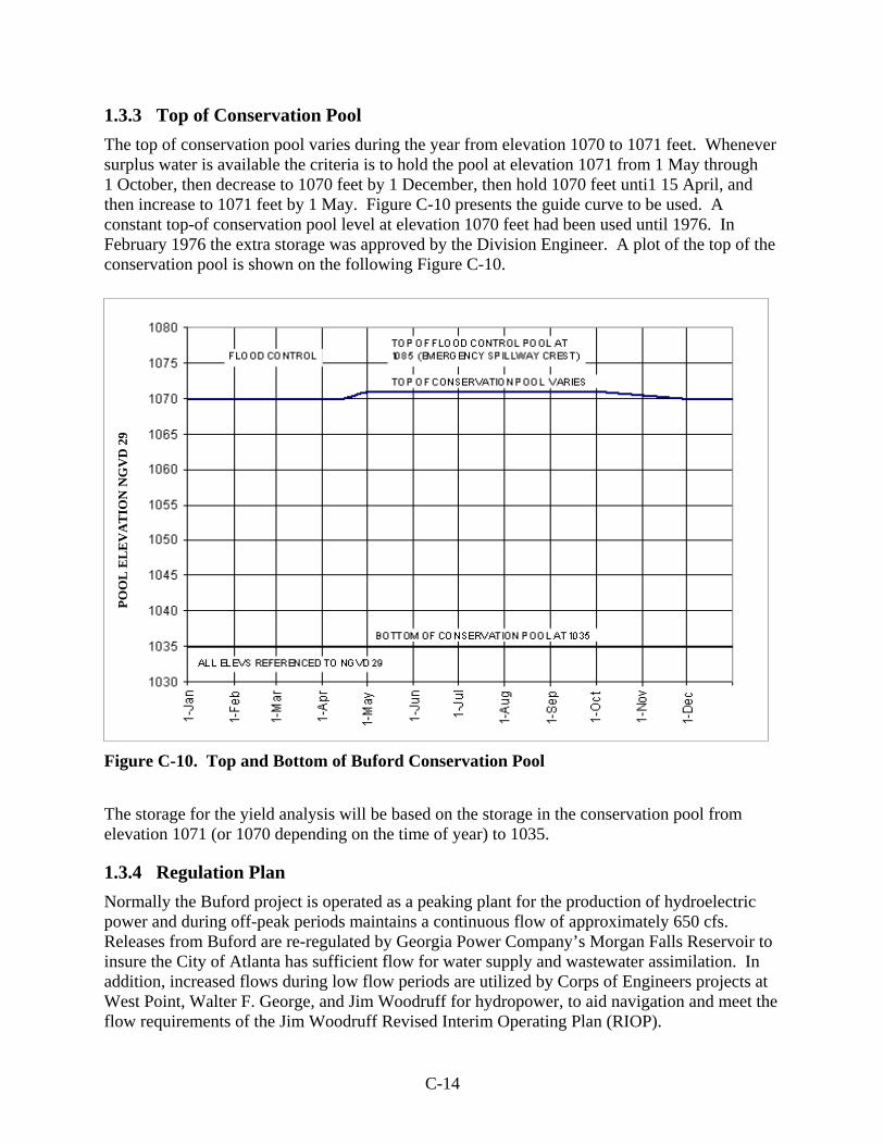
C-14


The top of conservation pool varies during the year from elevation 1070 to 1071 feet. Whenever surplus water is available the criteria is to hold the pool at elevation 1071 from 1 May through 1 October, then decrease to 1070 feet by 1 December, then hold 1070 feet unti1 15 April, and then increase to 1071 feet by 1 May. Figure C-10 presents the guide curve to be used. A constant top-of conservation pool level at elevation 1070 feet had been used until 1976. In February 1976 the extra storage was approved by the Division Engineer. A plot of the top of the conservation pool is shown on the following Figure C-10.

Figure C-10. Top and Bottom of Buford Conservation Pool The storage for the yield analysis will be based on the storage in the conservation pool from elevation 1071 (or 1070 depending on the time of year) to 1035.


Normally the Buford project is operated as a peaking plant for the production of hydroelectric power and during off-peak periods maintains a continuous flow of approximately 650 cfs. Releases from Buford are re-regulated by Georgia Power Company’s Morgan Falls Reservoir to insure the City of Atlanta has sufficient flow for water supply and wastewater assimilation. In addition, increased flows during low flow periods are utilized by Corps of Engineers projects at West Point, Walter F. George, and Jim Woodruff for hydropower, to aid navigation and meet the flow requirements of the Jim Woodruff Revised Interim Operating Plan (RIOP).

PO

OL

EL

EV

AT

ION

NG

VD

29

C-15


Observed daily inflow, outflow (discharge), and pool elevation data for the period of record starting in Jan 1958, just as the pool was filling through the present (Oct 2009) are available. The data are presented in the following Figure C-11.


The existing unimpaired flow data set was updated through 2008 for use in the yield analysis. The daily data was smoothed using 3-, 5-, or 7-day averaging to eliminate small negative values. Although this averaging affects the peak values, the volume is the same and the yield computations were done on the smoothed data. A plot of this smoothed unimpaired daily flow averaged over each year for the period of record 1939 – 2008 is shown in Figure C-12. Daily flows for critical drought periods are plotted in more detail in Figures C-13 – C-17.

C-16

cfs

-10,000

0

10,000

20,000

30,000

40,000

50,000

60,000

70,000

1960 1970 1980 1990 2000

Ele

v (f

t)

1,0301,0351,0401,0451,0501,0551,0601,0651,0701,075

BUFORD OBSERVED INFLOW BUFORD OBSERVED DISCHARGE

BUFORD OBSERVED ELEV

Figure C-11. Buford Inflow-Outflow-Pool Elevation (Jul 1957-Dec 2009)

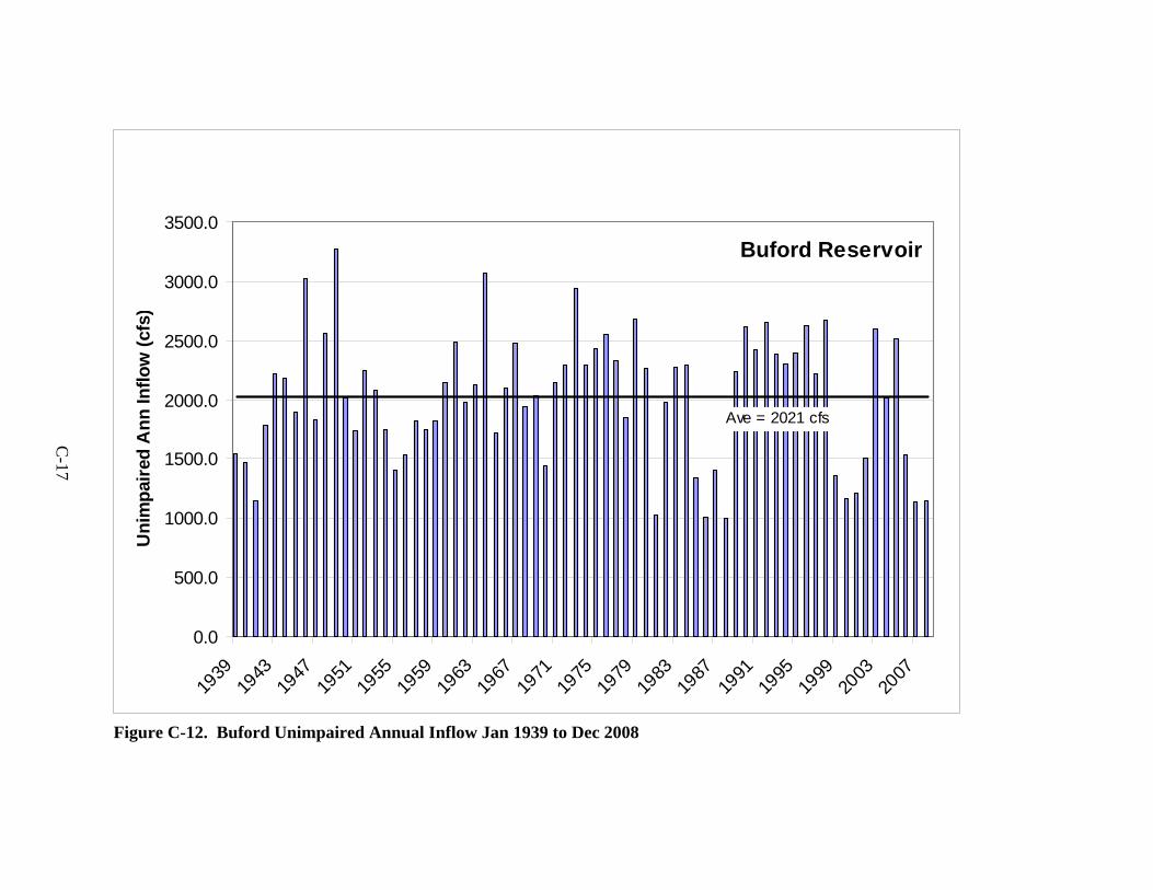
C-17

Buford Reservoir

0.0

500.0

1000.0

1500.0

2000.0

2500.0

3000.0

3500.0

1939

1943

1947

1951

1955

1959

1963

1967

1971

1975

1979

1983

1987

1991

1995

1999

2003

2007

Un

imp

aire

d A

nn

Infl

ow

(cf

s)

Ave = 2021 cfs

Figure C-12. Buford Unimpaired Annual Inflow Jan 1939 to Dec 2008

C-18

1939 1940 1941 1942 1943

Flo

w (

cfs)

-0

1,000

2,000

3,000

4,000

5,000

6,000

7,000

8,000

BUFORD UNIMP_CMA7[01JAN1939-31DEC2008] FLOW_INC-AVER

BUFORD UNIMP_CMA7[01JAN1939-31DEC2008] FLOW_INC-P25


BUFORD UNIMP_CMA7 FLOW_INC

Figure C-13. Buford Unimpaired Inflow – 1940’s Drought


C-19

1954 1955 1956 1957 1958

Flo

w (

cfs)

0

2,000

4,000

6,000

8,000

10,000

12,000







C-20

1984 1985 1986 1987 1988 1989

Flo

w (

cfs)

0

2,000

4,000

6,000

8,000

10,000

12,000







C-21

1998 1999 2000 2001 2002 2003

Flo

w (

cfs)

-2,000

-0

2,000

4,000

6,000

8,000

10,000

12,000





Figure C-16. Buford Unimpaired Inflow – 2000 Drought


C-22


2006 2007 2008

Flo

w (

cfs)

-0

1,000

2,000

3,000

4,000

5,000

6,000

7,000





Figure C-17. Buford Unimpaired Inflow – 2007 Drought


C-23

1.4 WEST POINT DAM (WEST POINT LAKE)

West Point Dam is located on the Chattahoochee River at mile 201.4 above the mouth and 3.2 miles north of West Point, Georgia. It is 146.9 river miles below Buford Dam, and 126.2 miles above Walter F. George Lock and Dam. The project was completed in May 1975. West Point Dam is a multiple-purpose project with major project purposes including flood control, hydroelectric power, navigation, recreation, fish and wildlife development and water quality. An aerial photo of the dam is shown in Figure C-18. Figure C-18. West Point Dam

1.4.1 Drainage Area

The drainage area above the dam is 3,440 square miles. The area is shown on the following Figure C-19. The operation of Buford Dam reduces peak stages about 10 feet to essentially non-damage stages at Morgan Falls Dam and for several miles downstream. The river bottoms are subject to some overbank flow during the infrequent floods at Vinings and in the northwest suburbs of Atlanta near Bolton. Between Bolton and West Point, a distance of about 100 river miles, there is no urban development in the floodplain. The Town of Franklin, 37 miles above West Point, is on high ground well above the flood zone. However, the effect of Buford Dam on floods decreases progressively downstream so that at West Point, peak stages are only slightly reduced. The Cities of West Point and Columbus, Georgia, and Lanett, Langdale, Riverview and Phenix City, Alabama, are all subject to flooding. Bankfull channel capacities downstream are 40,000 cfs at West Point and 32,000 cfs at Columbus. The West Point project provides a maximum flood storage of 391,000 acre-feet including the 221,000 acre-feet between elevations 628 and 635 available on a seasonal basis, and the 170,300 acre-feet between elevations 635 and 641 for induced surcharge operations.

C-24

Figure C-19. West Point Basin Map

C-25

For the single reservoir yield analysis in this report, only the area below Buford will be used for local inflow to West Point. This drainage area is the difference in the Buford and West Point drainage areas and is equal to 2,400 square miles. This West Point Basin below Buford area is shown in the following Figure C-20. Figure C-20. Incremental Drainage Basin Map for Federal Projects on the ACF

C-26

1.4.2 Features

The West Point Dam is a concrete gravity type structure with rolled earthfill embankments joining the high ground on the east and west sides of the river. The total length of the concrete dam and earth embankments is 7,250 feet. At the top of the structures, elevation 652 feet above mean sea level, the length of the concrete portion of the dam is 896 feet. The principal structures that make up the concrete dam are an intake-powerhouse structure, a non-overflow section, a gated spillway located in the main river channel, and a left embankment retaining wall which supports the earth embankment on the east abutment.

1.4.2.1 Non-Overflow Section

The non-overflow section is 185 feet long and forms the tie between the earth embankment on the west side of the river and the powerhouse intake section. The length of the non-overflow is determined by the clearance required between the terminal cone slopes and the powerhouse intake.

1.4.2.2 Spillway Section

The spillway section is a gravity type ogee section 350 feet long with crest at elevation 597. The spillway contains six tainter gates, each 50 feet wide and 41 feet high, between 10-foot thick piers supported on the overflow section.

1.4.2.3 Powerhouse and Intake

The powerhouse and intake structure are integrated into a reinforced concrete unit which acts as a part of the dam. The structure is 321 feet in length and consists of five monoliths located between the spillway and non-overflow section. The intake structure provides waterway openings for three main generating units (two to be installed initially and one for a future unit) and one small generating unit to provide continuous minimum flow releases. The main turbines are propeller type with concrete semi-spiral cases. The small was selected to give maximum efficiency while discharging 675 cfs at any head.

1.4.2.4 Reservoir

The reservoir has a total storage capacity of 774,800 acre-feet at full flood control pool, elevation 641 feet, and covers an area of 31,800 acres. At full conservation pool, elevation 635 feet, the reservoir covers 25,900 acres and has a total storage capacity of 604,500 acre-feet; at minimum conservation pool, elevation 620 feet, the area covered is 15,500 acres with storage capacity of 298,400 acre-feet. Area-capacity curves are shown on Table C-6 and Figure C-21. Conservation storage varies seasonally from 143,900 acre-feet to 306,100 acre-feet between a minimum elevation of 620 feet and a top of conservation pool elevation varying from 628 to 635 feet. Although the top of the flood control pool is 641 feet, only the conservation pool will be used in the yield analysis.

C-27

Table C-6. West Point Reservoir Area and Capacity

Pool Elev Total Area Total Storage (ft NGVD 29) (ac) (ac-ft)

*620 15,512 298,396 621 16,100 314,202 622 16,702 330,602 623 17,318 347,612 624 17,949 365,245 625 18,593 383,515 626 19,252 402,437 627 19,926 422,025

**628 20,615 442,295 629 21,318 463,260 630 22,037 484,937 631 22,771 507,340 632 23,520 530,485 633 24,286 554,387 634 25,067 579,062

***635 25,864 604,527 636 26,677 630,796 637 27,507 657,887 638 28,353 685,816 639 29,216 714,600 640 30,096 744,254

****641 30,993 774,798 642 31,907 806,246 643 32,838 838,618 644 33,788 871,930 645 34,755 906,200

* Minimum power pool ** Top of power pool - December through April *** Top of power pool - June through October **** Top of flood control pool

C-28

40,000.0 32,000.0 24,000.0 16,000.0 8,000.0 0.0

Area in Acres

570

580

590

600

610

620

630

640

Pool

Ele

vatio

n in

Fee

t abo

ve N

GV

D29

0 200,000 400,000 600,000 800,000 1,000,000Capacity in Acre-Feet

Area-Capacity CurveCapacityArea

Figure C-21. West Point Area – Capacity Curves

C-29


The top of conservation pool varies during the year from elevation 628 to 635 feet. Whenever surplus water is available the criteria is to hold the pool at elevation 635 from 1 June through 1 November, then decrease to 628 feet by 15 December, then hold 628 feet unti1 15 February, and then increase to 635 feet by 1 June, as shown in Figure C-22.


Normally the West Point project will be operated as a peaking plant for the production of hydroelectric power and during off-peak periods will maintain a continuous flow of 675 cfs. During low-water periods such regulation will provide increased flow downstream for navigation, water supply, water quality requirements and other purposes.

BOTTOM OF CONSERVATION POOL AT 620

1-Ja

n

1-F

eb

1-M

ar

1-A

pr

1-M

ay

1-Ju

n

1-Ju

l

1-A

ug

1-S

ep

1-O

ct

1-N

ov

1-D

ec

615

620

625

630

635

640

645

PO

OL

ELE

VA

TIO

N IN

FT

NG

VD

29

ALL ELEVS REFERENCE TO NGVD

615

620

625

630

635

640

645

TOP OF FLOOD CONTROL AT 641

FLOOD CONTROL

TOP OF CONSERVATION POOL VARIES 628-635

Figure C-22. Top and Bottom of West Point Conservation Pool The storage for the yield analysis will be based on the storage in the conservation pool from elevation 635 (or 628 depending on the time of year) to 620.

C-30


Observed daily inflow, outflow (discharge), and pool elevation data for the period of record starting in May 1975, just as the pool was filling through the present (Oct 2009) are available. The data are presented in the following Figure C-23.

1.4.6 Unimpaired Flow The existing unimpaired flow data set was updated through 2008 for use in the yield analysis. The daily data was smoothed using 3-, 5-, or 7-day averaging to eliminate small negative values. Although this averaging affects the peak values, the volume is the same and the yield computations were done on the smoothed data. A plot of this smoothed unimpaired daily flow averaged over each year for the period of record 1939 – 2008 is shown in Figure C-24. Daily flows for critical drought periods are plotted in more detail in Figures C-25 – C-29.

C-31

cfs

0

20,000

40,000

60,000

80,000F

LOW

010,00020,00030,00040,00050,00060,00070,000

1980 1985 1990 1995 2000 2005

Ele

v (f

t)

620

625

630

635

640

WEST-POINT OBSERVED INFLOW WEST-POINT OBSERVED DISCHARGE

WEST-POINT OBSERVED ELEV

Figure C-23. West Point Inflow-Outflow-Pool Elevation (Jan 1975-Dec 2009)

C-32

West Point Reservoir

0.0

1000.0

2000.0

3000.0

4000.0

5000.0

6000.0

7000.0

8000.0

9000.0

10000.0

1939

1943

1947

1951

1955

1959

1963

1967

1971

1975

1979

1983

1987

1991

1995

1999

2003

2007

Un

imp

aire

d A

nn

ual

Infl

ow

(cf

s)

Ave =5466 cfs

Figure C-24. West Point Unimpaired Annual Inflow Jan 1939 to Dec 2008

C-33

1939 1940 1941 1942 1943

Flo

w (

cfs)

0

5,000

10,000

15,000

20,000

25,000

30,000

35,000

WEST POINT R UNIMP_CMA[04JAN1939-31DEC2008] FLOW_CUM-AVER

WEST POINT R UNIMP_CMA[04JAN1939-31DEC2008] FLOW_CUM-P25


WEST POINT R UNIMP_CMA FLOW_CUM

Figure C-25. West Point Unimpaired Inflow – 1940’s Drought; 75th Percentile, Average and 25th Percentile Flow


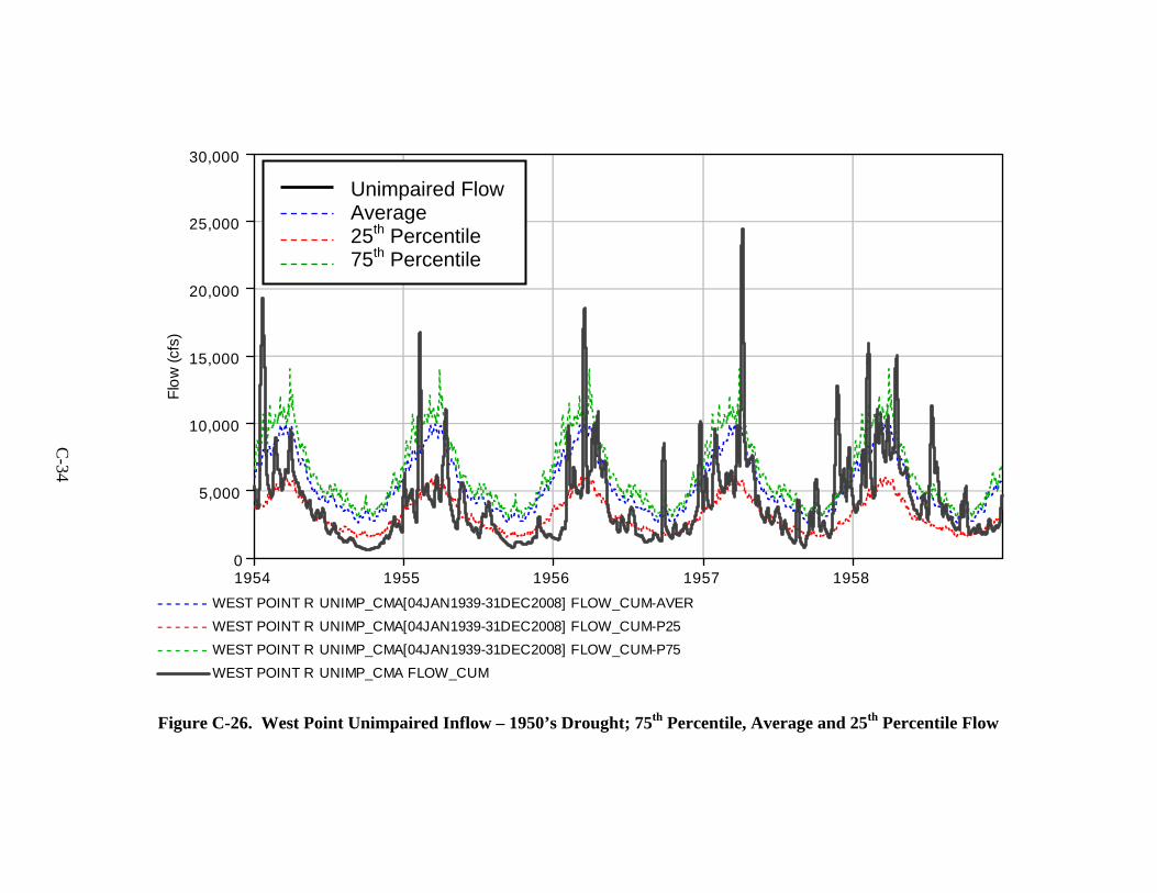
C-34

1954 1955 1956 1957 1958

Flo

w (

cfs)

0

5,000

10,000

15,000

20,000

25,000

30,000







C-35

1984 1985 1986 1987 1988 1989

Flo

w (

cfs)

0

5,000

10,000

15,000

20,000

25,000

30,000

35,000







C-36

1998 1999 2000 2001 2002 2003

Flo

w (

cfs)

0

5,000

10,000

15,000

20,000

25,000

30,000

35,000

40,000

45,000





Figure C-28. West Point Unimpaired Inflow – 2000 Drought; 75th Percentile, Average and 25th Percentile Flow


C-37


2006 2007 2008

Flo

w (

cfs)

0

2,000

4,000

6,000

8,000

10,000

12,000

14,000

16,000





Figure C-29. West Point Unimpaired Inflow – 2007 Drought; 75th Percentile, Average and 25th Percentile Flow


C-38

1.5 WALTER F. GEORGE DAM (LAKE EUFAULA) Walter F. George Lock and Dam is located on the Chattahoochee River at mile 75, approximately one mile north of Fort Gaines, Georgia and approximately 1.6 miles upstream from the Georgia State Highway 37 bridge. The dam crosses the Alabama-Georgia state line with the earth dike on the west bank entirely in Henry County, Alabama. The earth dike on the east is entirely in Clay County, Georgia. The project was completed in June 1963. Walter F. George Dam is a multiple-purpose project with major project purposes including, hydroelectric power, navigation, recreation, fish and wildlife development and water quality. The project was not designed for flood control. An aerial photo of the dam is shown in Figure C-30. Figure C-30. Walter F. George Dam

1.5.1 Drainage Area

The drainage area above Walter F. George Lock and Dam is 7,460 square miles. In the drainage area above Walter F. George Lock and Dam there are nine power developments and two multiple-purpose dams. Seven of the power projects are owned and operated by the Georgia Power Company. They are: Morgan Falls, Langdale, Riverview, Bartletts Ferry, Goat Rock, Oliver, and North Highlands. The City Mills Dam and Eagle and Phenix Mills Dam are independently owned and operated. These are very low head projects which have no effect on river hydraulics. Buford and West Point Dams are federal projects operated by the Corps of Engineers and are multiple-purpose dams that provide flood protection, production of hydroelectric power, water supply, recreation, instream flow, and increased flows for navigation during low-flow seasons. The drainage area and federal and Georgia Power Company dams are shown on the following Figure C-31.

C-39

Figure C-31. Walter F. George Basin Map

C-40

For the single reservoir yield analysis in this report, only the area below West Point was used for local inflow to Walter F. George. This drainage area is the difference in the West Point and Walter F. George drainage areas and is equal to 4,020 square miles. This Walter F. George Basin below West Point area is shown in the following Figure C-32.

Figure C-32. Incremental Drainage Basin Map for Federal Projects on the ACF

C-41


The dam consists of a powerhouse, a gated spillway, a lock in and adjacent to the original river channel, and earth dikes extending to high ground on both banks. The lock is 82 by 450 feet with a maximum lift of 88 feet. The project has a 130,000 kW power plant with appurtenances, and a reservoir extending up the Chattahoochee River 85 miles to Columbus, Georgia and Phenix City, Alabama. The reservoir provides a nine-foot minimum depth for navigation from the dam to Columbus and Phenix City. The principal features of the structure are, from left to right bank, an earth dike, the navigation lock, the concrete gated spillway, the powerhouse with intake section constituting part of the dam, and an earth dike.

1.5.2.1 Dam

Overall length of the structure including the lock and powerhouse sections is 13,585 feet, or 2.6 miles.

1.5.2.2 Reservoir

The reservoir at maximum summer operating level (conservation pool) of elevation 190, covers an area of 45,180 acres and has a total storage of 934,400 acre-feet. The pool extends up the Chattahoochee River 85 miles to Columbus, Georgia. At the minimum operating level (conservation pool), elevation 184, the reservoir covers an area of 36,375 acres and has a total storage of 690,000 acre-feet. Area and capacity curves are shown on Figure C-33 and in Table C-7.

80,000 70,000 60,000 50,000 40,000 30,000 20,000 10,000 0

Area in Acres

100

110

120

130

140

150

160

170

180

190

200

Pool

Ele

vatio

n in

Fee

t abo

ve N

GV

D29

0 200,000 400,000 600,000 800,000 1,000,000 1,200,000 1,400,000 1,600,000


Area-Capcity CurveCapacity

Area

Figure C-33. Walter F. George Area – Capacity Curves

C-42

Table C-7. Walter F. George Reservoir Area and Capacity

Pool Elev Total Area Total Storage (ft NGVD 29 (ac) (ac-ft)

100 8 10 105 248 550 110 587 2,610 115 902 6,340 120 1,248 11,680 125 1,550 18,670 130 1,894 27,240 135 2,375 37,920 140 2,966 51,210 145 3,720 67,830 150 4,895 89,100 155 6,815 118,140 160 10,624 161,500

*163 12,815 196,700 165 14,501 224,000 170 19,457 308,700 175 24,556 419,000 180 30,577 556,300 181 31,897 587,600 182 33,396 620,200 183 34,880 654,400 184 36,375 690,000 185 37,784 727,100 186 39,210 765,600 187 40,735 805,500

**188 42,210 847,100 189 43,665 890,000

***190 45,181 934,400 191 46,850 980,500 192 48,615 1,028,100 193 50,356 1,077,600 194 52,250 1,129,000 195 54,045 1,182,100 196 55,975 1,237,100 197 57,800 1,294,000 198 59,650 1,352,700 199 61,528 1,413,300 200 63,375 1,475,800

* Crest of gated spillway ** Top of power pool - December through April *** Top of power pool - June through September

C-43


The top of conservation pool varies during the year from elevation 188 to 190 feet. Whenever surplus water is available the criteria is to hold the pool at elevation 190 from 1 June through 31 October, then decrease to 188 feet by 1 December, then hold 188 feet unti1 1 May, and then increase to 190 feet by 1 June, as shown in Figure C-34.


The Walter F. George pool is regulated between the minimum pool elevation 184 and 190. The pool may rise above elevation 190 for short periods of time during high flow periods. A major operating constraint is the structural limitation that the difference between the headwater and tailwater must not exceed 88 feet at any time. In addition to reservoir constraints, downstream water needs will, at times, require outflow from Walter F. George to be fairly evenly distributed throughout each week.


ALL ELEVS REFERENCE TO NGVD 29

1-Ja

n

1-F

eb

1-M

ar

1-A

pr

1-M

ay

1-Ju

n

1-Ju

l

1-A

ug

1-S

ep

1-O

ct

1-N

ov

1-D

ec

182

184

186

188

190

192

194

196

PO

OL E

LEV

AT

ION

IN F

T N

GV

D29

TOP OF DAM


182

184

186

188

190

192

194

196

Figure C-34. Top and Bottom of Walter F. George Conservation Pool The storage for the yield analysis will be based on the storage in the conservation pool from elevation 184 to 188 - 190 (depending on the time of year).

C-44


Observed daily inflow, outflow (discharge), and pool elevation data for the period of record starting in January 1964, just after the pool filled, through the present (Oct 2009) are available. The data are presented in the following Figure C-35.


The existing unimpaired flow data set was updated through 2008 for use in the yield analysis. The daily data was smoothed using 3-, 5-, or 7-day averaging to eliminate small negative values. Although this averaging affects the peak values, the volume is the same and the yield computations were done on the smoothed data. A plot of this smoothed unimpaired daily flow averaged over each year for the period of record 1939 – 2008 is shown in Figure C-36. Daily flows for critical drought periods are plotted in more detail in Figures C-37 – C-41.

C-45

cfs

020,000

40,000

60,000

80,000

100,000F

LOW

-0

20,000

40,000

60,000

80,000

1965 1970 1975 1980 1985 1990 1995 2000 2005

Ele

v (f

t)

184

188

192

GEORGE OBSERVED INFLOW GEORGE OBSERVED DISCHARGE

GEORGE OBSERVED ELEV

Figure C-35. Walter F. George Inflow-Outflow-Pool Elevation (Jan 1964-Dec 2009)

C-46

W.F. George Reservoir

0

2000

4000

6000

8000

10000

12000

14000

16000

18000

1939

1943

1947

1951

1955

1959

1963

1967

1971

1975

1979

1983

1987

1991

1995

1999

2003

2007

Un

imp

aire

d A

nn

ual

Infl

ow

(cf

s)

Ave = 9845 cfs

Figure C-36. Walter F. George Unimpaired Annual Inflow Jan 1939 to Dec 2008

C-47

1939 1940 1941 1942 1943

Flo

w (

cfs)

0

10,000

20,000

30,000

40,000

50,000

60,000

70,000

80,000

W.F.GEORGE UNIMP_CMA[07JAN1939-31DEC2008] FLOW_CUM-AVER

W.F.GEORGE UNIMP_CMA[07JAN1939-31DEC2008] FLOW_CUM-P25


W.F.GEORGE UNIMP_CMA FLOW_CUM

Figure C-37. Walter F. George Unimpaired Inflow – 1940’s Drought; 75th Percentile, Average and 25th Percentile Flow


C-48

1954 1955 1956 1957 1958

Flo

w (

cfs)

0

5,000

10,000

15,000

20,000

25,000

30,000

35,000

40,000

45,000

50,000







C-49

1984 1985 1986 1987 1988 1989

Flo

w (

cfs)

0

5,000

10,000

15,000

20,000

25,000

30,000

35,000

40,000







C-50

1998 1999 2000 2001 2002 2003

Flo

w (

cfs)

0

10,000

20,000

30,000

40,000

50,000

60,000

70,000

80,000

90,000

100,000





Figure C-40. Walter F. George Unimpaired Inflow – 2000 Drought; 75th Percentile, Average and 25th Percentile Flow


C-51


2006 2007 2008

Flo

w (

cfs)

-5,000

-0

5,000

10,000

15,000

20,000

25,000

30,000





Figure C-41. Walter F. George Unimpaired Inflow – 2007 Drought; 75th Percentile, Average and 25th Percentile Flow


C-52

1.6 ResSim MODELING

The ResSim model for the ACF Basin is shown below in Figure C-42.

Figure C-42. ACF ResSim Model Schematic

C-53

ResSim version 3.2 Dev, November 2009 was utilized using the ResSim Watershed "ACF2009-Yield" and the network "ACF Yield". The ACF ResSim model includes four reservoirs, 19 non-reservoir locations and three diversion destinations. The fourth reservoir, Jim Woodruff, is run-of-river and not included in the yield analysis. Physical characteristics of each reservoir incorporated into the model using the latest published reservoir operation manual. Yield computations are dependent on the conservation storage and hydrology. The regulation plan section for each reservoir above describes the conservation storage. The ResSim operation set only includes the diversion yield rules and the downstream flood control rules. Reservoir guidelines for determining releases are defined using the operation set. Method C (System Yield) also includes tandem rules in the operation set for the system yield analysis from Walter F. George. Simulations were created for each of the five indentified drought periods. The beginning and end period was selected to capture the drawdown and refill of all projects. Buford, having the greatest amount of storage and smallest drainage area, determined the duration of the simulation period. Each yield method (A, B and C) includes one simulation for each of five drought periods. A total of 40 simulations were run. This included 15 simulations under Method A, 15 simulations under Method B and 10 simulations under Method C (5 without diversion and 5 with diversions). Each simulation determined the yield for a particular reservoir and drought period. Simulation naming uses the drought label from Table C-8. For example Method A simulation name for the 1980 drought is “1980 wo Div”, Method B is “1980 w Div” and Method C is “1980 System Yield”.

Table C-8. Drought Periods

Drought Periods Label

1940-1941 1940

1954-1958 1950

1984-1989 1980

1999-2003 2000

2006-2008 2007

Method A does not include the net river withdrawals and Method B does include the net river withdrawals in the yield determination. Each storage reservoir has a different operating set for the Method A and B alternatives, YieldNoDiv and YieldWDiv respectively. For Methods A and B the upstream reservoir is the primary reservoir and the yield is met first before proceeding downstream. Projects are full at the beginning of the drought period simulation. None of the yield is returned to the system. This assumes that the yield is diverted from the system and is consumptively used. For instance, on the ACF, this means that the yield computed at Buford was not counted as inflow to West Point, downstream. This methodology determines the conservative individual project yield. As mentioned in the “Methods Employed in Critical Yield Analysis” section, for the Method C simulations the reservoirs are operated together to compute a system yield at Walter F. George.

C-54

A diversion outlet is added to each of the three reservoirs (Buford, West Point and Walter F. George). Water from the reservoir is diverted through the outlet to a dummy location not connected to the system. None of the diverted water is returned to the system. The yield represents the maximum continuous flow of water through this outlet during one of the five drought periods using all available conservation storage.

1.7 RESULTS

Table C-9 below presents the results from each of the simulations for Method A, and the pool elevations and yield flow values are presented graphically in Figures C-43 – C-45. The flow represents the total release from the reservoir. When the flow hydrograph rises above the constant yield value, flows are released through the reservoir.

Table C-9. ACF Project Yield Analysis without River Diversions, Method A

Drought Period Project 1940 1950 1980 2000 2007 Critical Yield

Lanier 1,776 1,802 1,465 1,518 1,631 1,465 West Point 1,736 1,359 1,746 1,538 1,167 1,167 Walter F. George 1,903 1,589 1,424 785 572 572

Method A critical yield for Buford is 1,465 cfs and the critical period is the 1980’s drought period Method A critical yield for West Point is 1,167 cfs and the critical period is the 2007 drought period Method A critical yield for Walter F. George is 572 cfs and the critical period is the 2007 drought period

Figure C-43. Buford Critical Yield Result, Method A (No Diversions)

Legend


C-55

Figure C-44. West Point Critical Yield Result, Method A (No Diversions)

Figure C-45. Walter F. George Critical Yield Result, Method A (No Diversions)

Legend


Legend


C-56

The drawdown period for each drought period is listed in Table C-10.

Table C-10. ACF Yield Drawdown Period

Drought Label

Buford

West Point

Walter F. George

1940's Jun 1939 - Feb 1946 Apr 1941 - Jan 1942 May 1941 - Dec 1941

1950's Apr 1954 - Apr 1962 May 1954 - Feb 1955 May 1954 - Feb 1955

1980's Mar 1985 - Mar 1990 Mar 1986 - Dec 1986 May 1986 - Nov 1986

2000 Jun 1998 - Sep 2004 Apr 2000 - Feb 2001 Apr 2000 - Dec 2000

2007 Mar 2006 – Oct 2009* Mar 2007 - Feb 2008 Apr 2007 - Jan 2008 * Estimated based on actual refill Table C-11 below captures the impact of net year 2007 river withdrawals above the lakes from the Chattahoochee River and tributaries. Graphical results of the pool elevation and yield are presented in Figures C-46, C-47, and C-48. As expected the yield values are reduced because the inflow into the reservoirs is reduced by the river withdrawal amounts. The critical yield reduction for Buford, West Point and Walter F. George is 0.4%, 23.7% and 17.9% respectfully. Lake Lanier does not refill during the simulation period because unimpaired flow data through 2009 was not available at the time of analysis. The Corps will run the analysis through 2009 when flow data becomes available.

Table C-11. ACF Projects Yield Analysis with River Diversions, Method B

Drought Period Project 1940 1950 1980 2000 2007 Critical Yield

Lanier 1,772 1,798 1,460 1,513 1,628 1,460

West Point 1,449 1,077 1,454 1,230 891 891

Walter F. George 1,763 1,496 1,317 682 470 470 Method B critical yield for Buford is 1,460 cfs and the critical period is the 1980’s drought period Method B l yield for West Point is 891 cfs and the critical period is the 2007 drought period Method B yield for Walter F. George is 470 cfs and the critical period is the 2007 drought period

C-57

Figure C-46. Buford Critical Yield Result, Method B (With Diversions) Figure C-47. West Point Critical Yield Result, Method B (With Diversions)

Legend


Legend


C-58

Figure C-48. Walter F. George Critical Yield Result, Method B (With Diversions) Table C-12 presents the results from ACF system analysis, Method C. The table shows that, using the 2007 river diversions, the system yield is reduced 16%, from 4370 cfs to 3683 cfs. Graphical results are presented in Figure C-49 and Figure C-50.

Table C-12. ACF System Yield Analysis, Method C

Drought Period

Project 1940 1950 1980 2000 2007 Critical Yield

System with Diversions 5,471 4,616 4,671 4,019 3,683 3,683

System without Diversions 6,124 5,231 5,338 4,738 4,370 4,370

Legend


C-59

Legend


Figure C-49. System Critical Yield Result, Method C (No Diversions)

Buford Reservoir Release

West Point Reservoir Release

C-60

Legend


Figure C-50. System Critical Yield Result, Method C (With Diversions)

Buford Reservoir Release

West Point Reservoir Release

Appendix D

Prior Reports and References

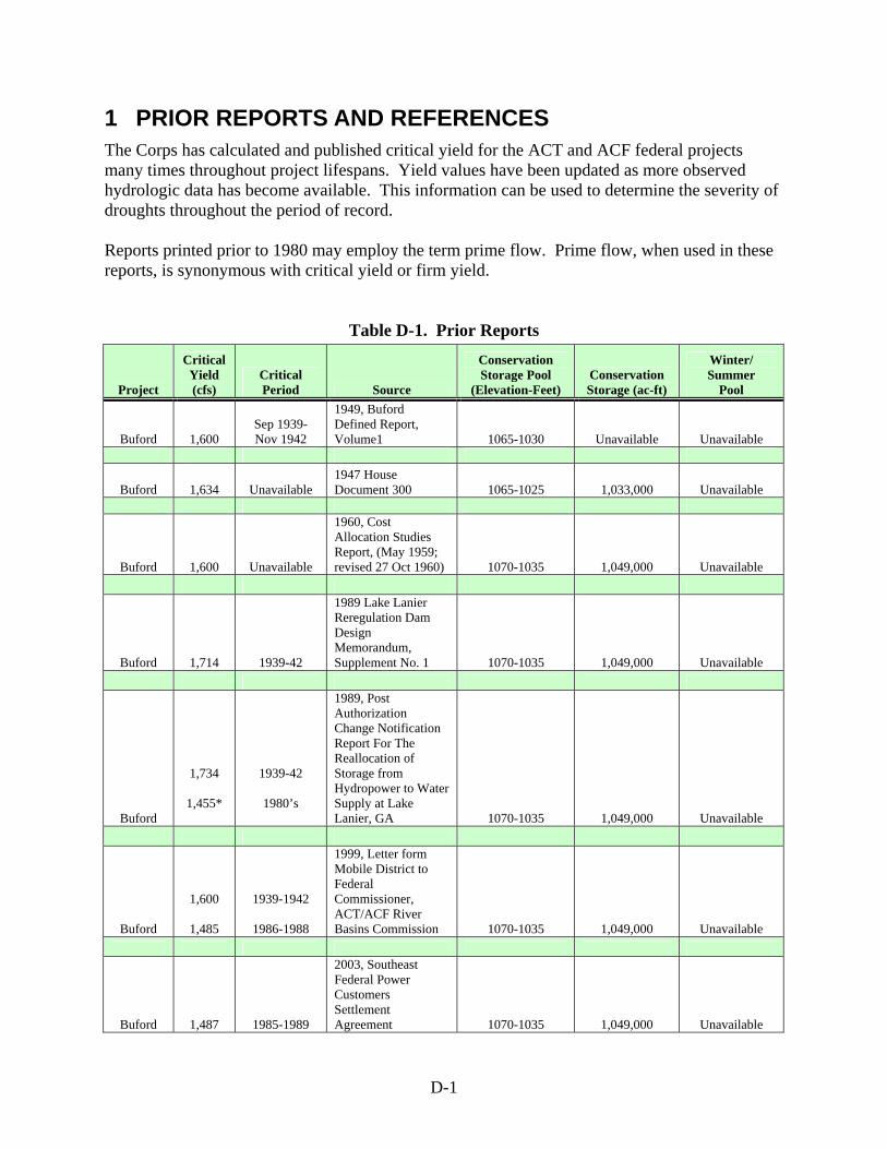
D-1

1 PRIOR REPORTS AND REFERENCES The Corps has calculated and published critical yield for the ACT and ACF federal projects many times throughout project lifespans. Yield values have been updated as more observed hydrologic data has become available. This information can be used to determine the severity of droughts throughout the period of record. Reports printed prior to 1980 may employ the term prime flow. Prime flow, when used in these reports, is synonymous with critical yield or firm yield.

Table D-1. Prior Reports

Project


Critical Period Source

Conservation Storage Pool

(Elevation-Feet) Conservation Storage (ac-ft)

Winter/ Summer

Pool

Buford 1,600 Sep 1939-Nov 1942

1949, Buford Defined Report, Volume1 1065-1030 Unavailable Unavailable

Buford 1,634 Unavailable 1947 House Document 300 1065-1025 1,033,000 Unavailable

Buford 1,600 Unavailable

1960, Cost Allocation Studies Report, (May 1959; revised 27 Oct 1960) 1070-1035 1,049,000 Unavailable

Buford 1,714 1939-42

1989 Lake Lanier Reregulation Dam Design Memorandum, Supplement No. 1 1070-1035 1,049,000 Unavailable

Buford

1,734

1,455*

1939-42

1980’s

1989, Post Authorization Change Notification Report For The Reallocation of Storage from Hydropower to Water Supply at Lake Lanier, GA 1070-1035 1,049,000 Unavailable

Buford

1,600

1,485

1939-1942

1986-1988

1999, Letter form Mobile District to Federal Commissioner, ACT/ACF River Basins Commission 1070-1035 1,049,000 Unavailable

Buford 1,487 1985-1989

2003, Southeast Federal Power Customers Settlement Agreement 1070-1035 1,049,000 Unavailable

D-2

Table D-1 (Cont’d). Prior Reports

Project


Critical Period Source

Conservation Storage Pool

(Elevation-Feet) Conservation Storage (ac-ft)

Winter/ Summer

Pool

West Point 2,570** 1950

1962, West Point Project Authority, House Document 570, 87th Congress

635-620 (Winter)

625-620 (Summer)

284,000 (Winter)

78,000

(Summer) 635/625

W. F. George 6,750** Unavailable

1960, Cost Allocation Studies Report (May 1959; Revised 27 Oct 1960) 190-184 Unavailable 185/190

Allatoona 1,220 1930-31

Definite Project Report for Allatoona Dam and Reservoir, 1941 848 - 788 456,000 Unavailable

Allatoona 1,160 1939-1942

1966, Cartersville, GA and 1963, Cobb County Marietta Storage Contracts

823-800 (Winter)

840-800

(Summer)

284,580 (Winter)

119,878

(Summer)

840/823

Allatoona 1,186

1,156

1,103

748

1942

1956

1981

1986

1999, Water Supply Reallocation Report

823-800 (Winter)

840-800

(Summer)

284,580 (Winter)

119,878

(Summer)

840/823

Allatoona 1159 Unavailable Storage Contract

Unavailable

Unavailable

Unavailable

Carters 424 Unavailable

Carters Lake Water Supply Reallocation Report, June 1989 1074 - 1022 Unavailable 1072/1074

Carters 550 1939-1942

Carters Dam Design Memorandum No. 4, Hydroelectric Power Capacity, 25 April 1962 1072 - 998 Unavailable 1070/1072

Carters 510 Unavailable

1991, City of Chatsworth, Georgia Storage Contract 1072 - 1022 134,900 Unavailable

*This represents a preliminary critical yield value that was calculated before the 1980’s drought ended. **Yield based on system analysis similar to Method C.

Appendix E

Drought Description

E-1

1 DROUGHT DESCRIPTIONS Five major, long-term (3 or more years) drought episodes have been identified during the period of record for the ACF and ACT River Basins in Alabama and Georgia. Each of these drought episodes displays differing spatial and temporal characteristics.

1.1 2006-2008

The 2006-08 drought was by far the most devastating drought recorded in Alabama and western Georgia. Precipitation declines began in December, 2005. These shortfalls continued through Winter 2006-07 and Spring 2007, exhibiting the driest winter and spring in the period of record. The drought reached peak intensity in 2007, resulting in a D-4 Exceptional Drought Intensity (the worst measured) throughout the Summer, 2007. Lakes and reservoirs dropped to the lowest levels ever recorded. Rainfall at Gainesville, Georgia (Lake Lanier) was only 20 inches for the entire year.

1.2 1998-2003

This period initiated the most recent multi-year drought "cycle". The drought reached peak severity in Summer, 2000, accompanied by all-time record high temperatures in many areas.

1.3 1984-1989

In the extreme northern portions of the ACF and ACT Basins, the 1984-89 drought was the worst drought known until that time. Precipitation from December 1985 through July 1986 was less than 40 percent of normal. Birmingham, Alabama and Chattanooga, Tennessee received only 17 inches of precipitation. The drought climaxed in July 1986, exacerbated by extremely high temperatures.

1.4 1954-1958

1954-58 was the most widespread, extreme and prolonged drought across the southern United States since the Dust Bowl of the 1930`s. The drought peaked in calendar year 1954; it was the driest of record statewide for Alabama since records began in 1895. Rainfall for 1954 was only 40 percent of normal across southeast Alabama.

1.5 1939-1943

Northwest Georgia experienced one of the driest springs of record in 1941. It was followed by drier than normal conditions across north Alabama during 1942-43.

alabama-coosa-tallapoosa (act) and ... district federal storage reservoir critical yield analyses...

Documents