airplanes and comparative advantage

1

printed 3/18/2005 4:33 PM version 3.0

Airplanes and Comparative Advantage

James Harrigan*

March 2005

Abstract Airplanes are a fast but expensive means of shipping goods, a fact which has implications for

comparative advantage. The paper develops a Ricardian three-country model with a continuum

of goods which vary by weight and hence transport cost. Comparative advantage depends on

relative air and surface transport costs across countries and goods, as well as stochastic

productivity. In the model, countries that are far from their export markets will have low wages

and tend to specialize in high value/weight products, which will be shipped on airplanes. Less

remote exporters will have higher wages, and will tend to specialize in low value/weight

products which will be sent by ship, train, or truck. These implications are confirmed using

detailed data on U.S. imports from 1990 to 2003. Distance from the US and air shipment are

associated with much higher import unit values.

* International Research Department, Federal Reserve Bank of New York, 33 Liberty Street, New York, NY 10045, [email protected]. This paper has benefited from audience comments at Ljubljana, Illinois, Michigan, Columbia, and the World Bank. I thank Jonathan Eaton, David Hummels and Stephen Redding for helpful conversations, and Christina Marsh for excellent research assistance. The views expressed in this paper are those of the author and do not necessarily reflect the position of the Federal Reserve Bank of New York or the Federal Reserve System.

1

1 Introduction

Countries vary in their distances from each other, and traded goods have differing physical

characteristics. As a consequence, the cost of shipping goods varies dramatically by type of good

and the route that it is shipped. A moments reflection suggests that these facts are probably

important for understanding international trade, yet they have been widely ignored by trade

economists. In this paper I focus on one aspect of this set of facts, which is that airplanes are a

fast but expensive means of shipping goods.

The fact that airplanes are fast and expensive means that they will be used for shipping

only when timely delivery is valuable enough to outweigh the premium that must be paid for air

shipment. They will also be used disproportionately for goods that are produced far from where

they are sold, since the speed advantage of airplanes over surface transport is increasing in

distance. In this paper I build a simple model that illustrates some implications of these

observations for specialization and wages: remote countries will have lower wages, and will

specialize in lightweight goods which are air shipped. Using a highly disaggregated database on

all U.S. imports from 1990 to 2003, I show empirically that distance generally and airplanes in

particular make a big difference in the composition of U.S imports.

There is a small, recent literature that looks at some of the issues that I analyze in this

paper. Limao and Venables (2002) model the interaction between specialization and trade costs,

illustrating how the equilibrium pattern of specialization involves a tradeoff between

comparative costs and comparative transport costs. Deardorff (2004) elegantly shows how

relative distance affects the trade pattern, arguing that local comparative advantage (defined as

autarky prices in comparison to nearby countries rather than the world as a whole) is what

matters in a world with trade costs. Evans and Harrigan (2005) develop a model of the demand

for timeliness, and show how the pattern of US apparel imports is influenced by the interaction

between relative distance and the relative value of timely delivery. Harrigan and Venables (2004)

further develop microfoundations for the demand for timely delivery, and show how timeliness

can lead to an incentive for agglomeration.

David Hummels has written a series of important empirical papers that directly motivated

this paper, as well as motivating Evans and Harrigan (2005) and Harrigan and Venables (2004).

Hummels (1999) shows that ocean freight rates have not fallen on average since World War 2,

and have often risen for substantial periods. By contrast, the cost of air shipment has fallen

2

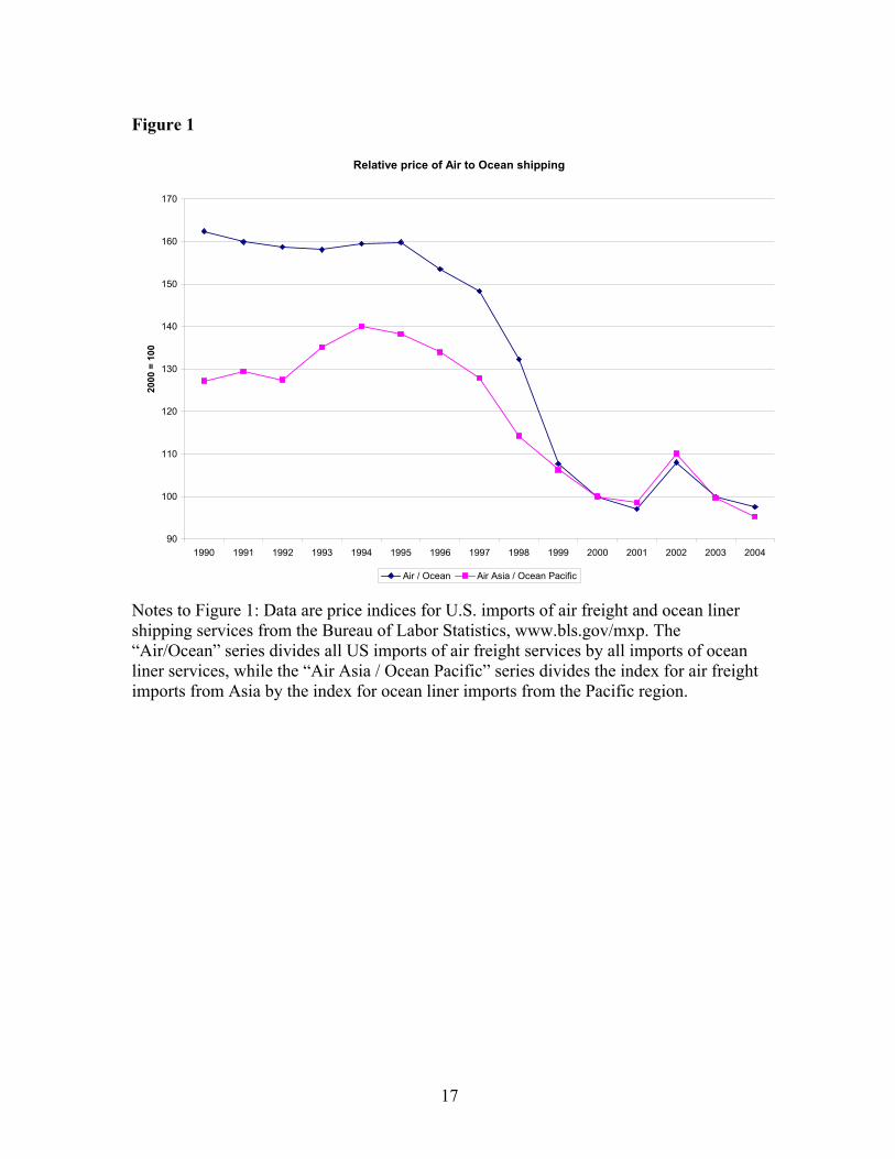
dramatically. Figure 1 shows that these trends have continued since 1990, with the relative price

of air shipping falling 40% between 1990 and 2004. Hummels (2001a) shows that shippers are

willing to pay a large premium for faster delivery, a premium that has little to do with the interest

cost of goods in transit1. Hummels (2001b) analyzes the geographical determinants of trade

costs, and decomposes the negative effect of distance on trade into measured and unmeasured

costs.

2 Airplanes and trade: theory

In the model there are three countries, 1, 2, and 3, which can be thought of as “United States”,

“Mexico” and “China”. Country 1 has a large technological advantage in a homogeneous

numeraire good, so in the equilibria that I examine it specializes in this good, which it produces

with a unit labor requirement of one. With 1’s wage as the numeraire, the FOB export price of

1’s good is also one2. 1 consumes the numeraire and imports from 2 and 3. Demand for the

numeraire and imports comes from a Cobb-Douglas utility function with expenditure share α on

total imports.

Countries 2 and 3 are identical except for distance from 1 and the size of their labor

forces. Both countries produce x, which they don’t consume, exporting all their output to 1, and

using the export revenues to buy the numeraire from 1. Producers in 2 and 3 face a choice of

shipping mode (air or surface). Air shipment is more costly, and depends on the weight of the

product being shipped. Despite its cost, air shipment may be profitable because goods shipped by

air can be sold for a premium over surface shipped goods. To formalize this tradeoff, let an index

z ∈ [0,1] order goods by increasing weight (and therefore increasing value/weight, though this

will be endogenous): good 0 is the lightest (computer chips), while good 1 is the heaviest (oil).

Surface shipping costs are the same for all goods, but airfreight iceberg costs ω(z) >1 are

increasing in weight and, therefore, increasing in z: good 0 is the cheapest to send by air, while

good 1 is the most expensive. Furthermore, the cost of air freight is the same regardless of where

1 By “the interest cost of goods in transit”, I mean the financial cost of having goods in transit before they can be sold. This opportunity cost equals the value of the good × daily interest rate × days in transit.

3

the flight originates, and to make the problem interesting assume

ω(z) > τ3 > τ2 > 1 for all z. (1)

Why would anybody pay for airfreight? The answer is, consumers like speedy delivery

for some reason, so that demand is higher for the same good when it is shipped by air. Some of

the reasons for such a preference are analyzed by Evans and Harrigan (2005) and Harrigan and

Venables (2004), but for the purposes of this model I will simply suppose that utility is higher for

goods that arrive by air. Let the set of goods shipped by air be A, with measure also given by A.

Subutility for imports is

( ( )) ln ( ) ln ( )z A z A

U x z a x z dz x z dz∈ ∉

= +∫ ∫ (2)

where a > 1 is the air-freight preference. The resulting demand functions are generalizations of

constant-expenditure-share Cobb-Douglas:

( )1( )

1 ( ) ( )a Lx z z A

aA A z p zα

ω= ⋅ ∈

+ −

(3)

( )

11( )1 ( )

Lx z z AaA A p z

ατ

= ⋅ ∉+ −

The relevant prices are inclusive of transport costs, which will depend on where the good is

produced and perhaps on weight.

Given these demands and the structure of transport costs, the next task is to determine the

equilibrium location of production. Perfect competition ensures FOB price = unit cost, but there

is a choice of shipping mode and consequent CIF price paid. When buying from location c,

consumers are willing to pay for airfreight as long as the relative marginal utility from timely

delivery exceeds the relative shipping cost, or

( )

c

z aωτ

≤ , c = 2, 3 (4)

Since FOB production costs are the same, competition among sellers means that they will ship

by air just in case this inequality is satisfied. I choose parameter values so that this never happens

for country 2 and sometimes does for country 3:

2 FOB stands for “free on board”, and refers to the price of the good before transport costs are added. CIF stands for “cost, insurance, and freight”, and refers to the price after transport costs

4

[ ]2 ( ) 0,1a z zτ ω< ∈

[ ]3 ( ) ,1a z z zτ ω< ∈ (5)

[ ]3( ) 0,z a z zω τ≤ ∈

The cutoff z is an endogenous variable which is determined by the relative cost of air and

surface shipping in country 3 only, given implicitly by

( )3a zτ ω= , (6)

and its determination is illustrated in Figure 2. Goods [ ],1z z∈ will never be shipped by air,

regardless of where they are produced, and I call these goods heavy. Light goods, [ ]0,z z∈ , will

be shipped by air if they are produced in 3, otherwise they will be shipped by surface from 2.

The boundary between heavy and light goods will change when surface or air transport costs

change, but it does not depend on comparative cost advantage, since it reflects only the decision

facing a producer in one country.

Production location and shipping mode are determined jointly. Define relative surface

transport costs, relative wages, and relative unit labor requirements respectively as

( ) ( )( )

22 2

3 3 3

, ,b zww b z

w b zτττ

≡ ≡ = (7)

For heavy goods, consumers in 1 buy from the lowest cost source, where costs are inclusive of

wages and transport costs. Therefore, goods are produced in 2 if and only if

τ2b2(z)w2 ≤ τ3b3(z)w3

or

[ ]( ) 1 ,1wb z z zτ ≤ ∈ . (8)

For light goods, we know that if they are produced in 3 they’ll be shipped by air, so the relevant

cost comparison is between surface in 2 and air in 3. But production cost is not the only

consideration, since consumers are willing to pay more for goods shipped by air. The relevant

cost comparison needs to be adjusted for this, and becomes

[ ]3 32 2 2

( ) ( )( ) 0,z b z wb z w z za

ωτ ≤ ∈

so production takes place in 2 if and only if

have been added.

5

[ ]2 ( ) 1 0,( )

wb z z zz a

τω

≤ ∈ (9)

These inequalities define the sets of heavy and light goods produced in each country:

[ ] ( ){ } [ ] ( ){ }2 3,1 | 1 , ,1 | 1H Hz z z wb z z z z wb zτ τ= ∈ ≤ = ∈ >

(10)

[ ] ( ) [ ] ( )2 32 2

( ) ( )0, | , 0, |L Lz zz z z wb z z z z wb za a

ω ωτ τ

⎧ ⎫ ⎧ ⎫= ∈ ≤ = ∈ >⎨ ⎬ ⎨ ⎬⎩ ⎭ ⎩ ⎭

Obviously, the set of goods produced in each country is the union of light and heavy goods

produced there. Note also that light goods produced in 3 are air shipped, so 3Lz A= . In an abuse

of notation, let the labels of these sets also denote their measure, so

2 3 2 31H H L Lz z z z z z+ = − + =

(11)

2 2 2 3 3 21H L H Lz z z z z z+ = + = −

I will treat labor productivity in good z as a random variable, and I adopt the modeling

strategy of Eaton and Kortum (2002). I simplify the Eaton-Kortum framework by focusing on

just two countries that have identical distributions of labor productivity (the inverse of the unit

labor requirement) drawn from a Fréchet distribution with parameters T > 0 and θ > 1. With this

distribution, the log of productivity has mean logTγθ

+ and standard deviation 6

πθ

, so that

smaller values of θ imply greater dispersion in productivity3.

With random productivity, the low-cost producer is probabilistic. Adapting Eaton and

Kortum’s equation (8) for my purposes gives a particularly simple expression for the probability

that country 2 is the supplier of heavy good z:

( )( ) ( ) ( )

[ ]2 22 2

2 2 3 3

1( ) ,11

H H wz z z

w w w

θ

θ θ θ

τπ π

τ τ τ

−= = = ∈

− −+ + (12)

This expression is quite intuitive: the probability that country 2 will supply any given heavy

goods is decreasing in 2’s relative wages and transport costs. The problem is slightly more

6

complex for lightweight goods for two reasons. The first is that country 3’s optimal shipping

mode for lightweight goods is air, and the transport cost for these goods depends on weight. The

second is that consumers in 1 are willing to pay a premium a > 1 for goods shipped by air. Using

equation (9) with the Fréchet distribution for productivities implies that the probability that

country 2 is the supplier of light good z is

( ) ( )

( ) ( )

2 22

3 32 2

1 [0, )( )

1( )

L wz z z

z w aw wa z

θ

θ θθ θ

τπ

ω ττ τω

−

−−

= = ∈⎛ ⎞ ⎛ ⎞+ +⎜ ⎟ ⎜ ⎟⎝ ⎠ ⎝ ⎠

(13)

The term 3

( )a

z

θτ

ω⎛ ⎞⎜ ⎟⎝ ⎠

in equation (13) is strictly greater than one, which implies ( )2 2L Hzπ π< for all

[0, )z z∈ . This result says that country 2 has a greater chance of supplying heavy goods than

lightweight goods, and the lighter the good the lower the chance that 2 will be the supplier. The

law of large numbers implies that for any interval of goods the average probability will be the

share of goods supplied by country 2, so I’ll refer to the π’s from now on as market shares. The

market shares for country 3 are of course just one minus the shares for country 2:

( )

( )( )

3 3

3

1 1,1 1

( )

H L zaw w

z

θθθ

π πττ τ

ω

−−−

= =⎛ ⎞+ + ⎜ ⎟⎝ ⎠

(14)

Figure 3 illustrates equations (12) and (13). Country 2’s market share is increasing in the

weight of the good ω(z) for all [0, )z z∈ . In this range, if a good is supplied by country 2 it is

sent by surface at a cost of τ2 while if it is supplied by 3 it is sent by air at a cost of ω(z). For

heavy goods z z≥ , both countries use surface transport, and country 2 has a transport cost

advantage since τ3 > τ2 . Equation (12) implies that if wages are the same, country 2 will have a

greater than 50% market share in heavy goods, but that within heavy goods 2’s market share is

constant.

To close the model I make wages endogenous. Factor market clearing requires that FOB

export revenue equals national income in country 2 and 3. For both countries, FOB revenue from

good z is the probability that it produces the good times country 1’s CIF expenditure on that

3 In terms of the Eaton-Kortum model, I assume that both countries have the same comparative advantage parameter Tc. The constants are γ = 0.577... and π = 3.14159.... See Eaton and Kortum

7

good, divided by the iceberg transport cost. Expenditure levels for good z are found by

multiplying equations (3) by p(z). Total expenditure on light goods is then the integral of

expenditure on each good over the range [ )0, z , and expenditure on heavy goods is the integral

over the range [ ],1z . Using these expenditure levels and the probabilities from (12) and (13),

the factor market clearing condition for country 2 becomes

( )

11 2 2

2 22 20

( )1

z L H

z

L zw L dz dzaA A

α π πτ τ

⎡ ⎤= +⎢ ⎥+ − ⎣ ⎦

∫ ∫

( )

( ) ( )1

2 20 3

1 1 1 11 11

( )

zL zdzaA A a ww

z

θ θθ

ατ ττ ττ

ω

⎡ ⎤⎢ ⎥

−⎢ ⎥= +⎢ ⎥+ − ⎛ ⎞ +⎢ ⎥+ ⎜ ⎟⎢ ⎥⎝ ⎠⎣ ⎦

∫ (15)

Similarly for country 3, export revenue is the sum of FOB revenue from air- and surface-shipped

goods:

( )

11 3 3

3 330

( )1 ( )

z L H

z

L zw L a dz dzaA A z

α π πω τ

⎡ ⎤= +⎢ ⎥+ − ⎣ ⎦

∫ ∫

( )( )

( )( )

11

30 3

1( ) 11 11

( )

z zL za dzaA A a ww

z

θ θθ

α ωττ ττ

ω

−

− −−

⎡ ⎤⎢ ⎥

−⎢ ⎥= +⎢ ⎥+ − ⎛ ⎞ +⎢ ⎥+ ⎜ ⎟⎢ ⎥⎝ ⎠⎣ ⎦

∫ (16)

The market clearing equations (15) and (16) along with equation (6) that defines z are three

equations in the three unknowns w2, w3, and z . With a solution to these three equations, the

other endogenous variables of the model (national income and trade flows) are obtained by

substitution.

The three equation system given by equations (6), (15) and (16) is highly nonlinear but

fairly simple economically. Intuitive results can be obtained by using a convenient functional

form for ω(z), 1

3( ) zz aω βτ += (17)

(2002) for more on the Fréchet distribution and its interpretation.

8

where the shift parameter β has a range of [a-1, 1]4. Recall that the condition for airfreight to be

profitable for country 3 in good z is 3( )z aω τ≤ . For low values of β air freight is always

profitable for country 3,

13 3(0) (1)a aβ ω τ ω τ−= → = =

while for high values it is never profitable:

23 31 (0) (1)a aβ ω τ ω τ= → = =

Substituting (17) into (6) gives the solution for z :

[ ]log 0,1log

zaβ

= − ∈

By varying β I can do comparative statics on the model’s equilibrium. Finding an analytical

solution for equilibrium wages is impossible, as the integrals in (15) and (16) can not be

evaluated analytically. Consequently, I solve the model for a numerical example (details of the

computations are in the Appendix).

As noted in the introduction, the long-term trend is for air transport costs to decline

relative to the cost of surface shipping (Figure 1). I model this as a proportionate shift down in

the cost of air transport ω(z). Figure 4 shows that falling air transport costs expand the range of

goods which are potentially shipped by air. The increase in z creates excess supply for country

2’s labor, as some goods formerly produced in 2 are now profitable to produce in 3 and send by

air. In the new equilibrium relative wages in 2 decline, and the resulting effects on market shares

are illustrated in Figure 5. Country 2 increases its market share in all heavy goods, where 2’s

now-lower wage improves its competitiveness, and loses market share in light goods, where the

lower cost of air shipping more than offsets the drop in 2’s wages.

Equilibrium wages as a function of the cost of air shipment are illustrated in Figure 6.

The figure is normalized so that wages in 2 are equal to one at β = 1, where air freight is

prohibitively expensive even for the lightest goods. As expected, a fall in air freight costs

(declining β) lowers the wage of 2 in both absolute and relative terms. Surprisingly, the initial

effect of a decline in air freight costs on w3 is negative. This is an instance of immiserizing

technological improvement: the increased supply of goods from 3 lowers their price by more

4 A further parameter restriction for this functional form is τ3 > aτ2 , which guarantees that airfreight is never profitable for country 2.

9

than the improvement in technology. As technology improves further, this terms of trade effect is

outweighed by the efficiency gain on inframarginal goods, so w3 increases. This result is partly

an artifact of the assumption of Cobb-Douglas expenditure by country 1, and with a more elastic

aggregate demand for imports the negative terms of trade effect of technological improvement

would diminish.

Whatever the effect on the absolute level of wages in 3, lower air freight costs inevitably

lower wages in 2. This happens because 2 faces greater competition from 3 but has no use for the

improved air shipping technology. The unambiguous winner is country 1, which gets lower

prices on all its imports from 2 and gets a wider range of air shipped goods from 3. In the case

where w3 actually falls, country 1 gets more than 100% of the global welfare gain from improved

technology: 1 gets both lower prices on all the goods it imports by surface and a wider selection

of air shipped goods.

2.4 The model’s prediction for trade data

For any given level of wages, the model delivers predictions about the cross-section of

goods imported by 1, and it is these predictions which will be the focus of the empirical analysis.

The first prediction has already been illustrated in Figure 3 : country 2 will have lower market

share in light-weight goods, and these light goods will be shipped by air when produced by 3.

More generally, the message of the model is that nearby countries will specialize in heavy goods

and faraway countries will specialize in light goods.

In the model all non-weight-related determinants of specialization are treated as random.

This is a useful modeling device but ignores what is known about the systematic influence of

factor endowments, development, country size, industry-level technology differences, etc on

comparative advantage. A transparent example is oil: the reason that Mexico exports oil to the

US and Japan does not has nothing to do with the fact that oil is heavy. In taking the model to the

data other determinants of specialization must be taken into account, at least statistically. The

prediction of the theory then acquires a ceteris paribus clause: all other things equal, nearby

countries will specialize in heavy goods.

Most import records report quantities as well as FOB values, which makes it possible to

construct unit values, defined as the dollar value of imports per physical unit. Since shipping

costs depend primarily on the physical characteristics of the good rather than on its value, low

10

value goods will be “heavy” in the sense of having a higher shipping cost per unit of value5. For

example, consider shoes. Quantities of shoes are reported in import data, and the units are

“number” as in “number of shoes”. Expensive leather shoes from Italy and cheap canvas

sneakers from China weigh about the same, but the former will have a much higher unit value. In

the context of the model, Italian leather shoes are “lighter” than Chinese fabric sneakers, in the

economically relevant sense that the former have lower transport costs as a share of value. The

model’s prediction can then be translated into a prediction about unit values: within a given

product category, nearby countries will tend to specialize in low-value goods. High-value goods

will tend to be produced in more distant locations and will be shipped by air.

3 Airplanes and trade: empirical evidence

The data used in this paper are derived from detailed import statistics collected by the

U.S. Customs Service and reported on CD-ROM. For each year from 1990, the raw data includes

information on the value, quantity (usually number or kilograms), and weight (usually in

kilograms) of U.S. imports from all sources. The data also include information on transport

mode and fees, including total transport charges broken down by air, vessel and (implicitly)

other, plus the quantity of imports that come in by air, sea, and (implicitly) land.6

The data are reported at the 10-digit Harmonized System (HS) level, which consists of

almost 17,000 separate categories in 2003. I aggregate this data for analysis in various ways. For

most of the descriptive charts and tables, I work with a broad aggregation scheme that updates

Leamer’s (1984) classification, which is reported in Table 1. For the regression analysis, I work

with the 6-digit HS categories, of which there were over 14,000 in 2003.

The unit value of imports is defined as the value of imports divide by the physical

quantity. The units measuring physical quantity vary by commodity, with the most common

being “number” (as in, number of cars) and kilograms (as in, kilograms of steel). For the

majority of records, there are two units reported, the first often number and the second invariably

weight; this makes it possible to distinguish between unit value and value to weight for a

particular import value.

5 The relationship between shipping cost and shipment value is estimated by Hummels and Skiba (2004), Table 1. They find that shipping costs increase less than proportionately with price.

11

3.1 Data description

Table 1 illustrates the great heterogeneity in the prevalence of air freight, as well as some

important changes over the sample. Many products come entirely or nearly entirely by surface

transport (oil, iron and steel, road vehicles) while others come primarily by air (computers,

telecommunications equipment, cameras, medicine). Scanning the list of products and their

associated air shipment shares hints at the importance of value to weight and the demand for

timely delivery in determining shipment mode.

Charts 1 to 10 illustrate the variation in air freight across regions and goods (the regional

aggregates are defined in Table 2, while the product aggregates correspond to the headings in

Table 1). Chart 1 shows that the about a quarter of US (non-oil) imports arrived by air in 2003,

up from 20% in 1990 (for brevity, in what follows I’ll call the proportion of imports that arrive

by air “air share”). Chart 2 shows that this average conceals great regional variation, which is

related to distance: essentially no imports come by air from Mexico and Canada, while Europe’s

air share is almost half by 2003, up from under 40% in 1990. East Asia’s air share increased by

about half from over the sample, from 20 to 30%. The airshare from the Caribbean and South

America was about one-fifth over the sample. Chart 3 shows that air shipment is concentrated in

manufactured goods, particularly labor-intensive manufactures and machinery (as Table 1 shows,

the capital-intensive aggregate is mainly steel and other metals, which are very heavy). The

biggest increase in air share came in chemicals, which (as Table 1 reveals) is accounted for by

the increasing importance of pharmaceuticals, which had an 80% air share in 2003.

The remaining Charts 4 through 10 show the evolution of air share by major regions and

product aggregates. The most notable fact about Chart 4 is the sharp increase in machinery’s air

share from East Asia, to levels similar to Europe’s by 2003 (Chart 5). Western and South Asia

(which is mainly the Indian subcontinent), shows a puzzling drop in the air share for labor

intensive manufactures, a drop also seen in the Caribbean (Chart 7). This may have to do with

the phenomenon documented by Evans and Harrigan (2005): as apparel production moved to

Mexico during the 1990s, the shift was concentrated in goods where timely delivery is important.

Essentially, U.S. apparel retailers who wanted timely delivery replaced air shipments from South

Asia and the Caribbean for surface shipments from next-door Mexico.

6 “other” transport modes include truck and rail, and are used exclusively on imports from Mexico and Canada.

12

Heavy capital-intensive goods have not shown any increase in air-share from any source

since 1990 (Chart 8), but lighter machinery imports became increasingly air shipped from East

Asia (Chart 9). Finally, the shift toward air shipment in chemicals from major suppliers was

world-wide, with the obvious exception of NAFTA (Chart 10).

Chart 11 shows import-weighted average transport charges for total imports and for air

shipped imports. There has not been much of a change in these numbers over the sample period,

with overall transport charges equal to about 5% of import value and air charges about 10%. But

as Hummels (2001b) emphasizes, these averages underestimate the true level of transport

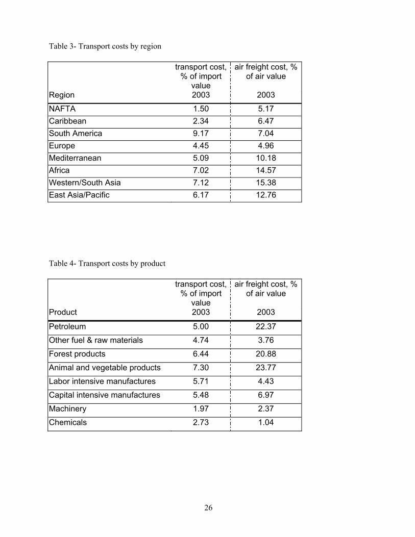
charges facing importers, since they reflect a cost-minimizing equilibrium. Tables 3 and 4

illustrate how weighted average transport costs vary by region and product category. Not

surprisingly, the products that have the highest air share, Machinery and Chemicals, have the

lowest air freight costs. In some of the categories, the average transport cost is lower for air than

overall, which of course reflects selection: very low value/weight items, which cost a lot to move

even by ship, don’t get put on planes.

3.2 Statistical results

The theory model of section 2 makes a number of predictions. The one I focus on here

concerns the price of imports across source countries: the model predicts that imports from

faraway countries will weigh less, and will have higher f.o.b. prices, than goods shipped from

nearby countries. Statistically, I investigate this by looking at variation in unit values across

exporters within 10-digit HS categories. The econometric model I use is

ict it t cv d other controls residualα β= + + + (18)

where

vict = log unit value of imports of product i from country c in year t

αit = fixed effect for 10-digit HS code i in year t

dc = distance of c from United States

Note that import values are measured f.o.b, so they do not include transport charges. The model

predicts βt > 0 in equation (18): across exporters within a 10-digit commodity category, more

distant exporters will sell products with higher unit values, controlling for other observable

country-specific factors which might affect unit values. When the units are kilograms, then the

prediction for unit values is a prediction about the value-weight ratio.

13

In the model, the effect of distance on unit values comes through a sorting effect which

leads to higher-valued goods being produced at greater distance and then shipped by air. To test

for the direct effect of air shipment on unit values, I estimate the model

1 2ict it t ict t cv a d other controls residualα β β= + + + + (19)

where

aict = share of imports of i from c that came by air in t.

Strictly speaking, the model predicts β1t = 0 and β2t > 0 in equation (19): controlling for

transport mode, distance should have no further effect on unit values. But if non-air transport

costs per unit are increasing in distance (as they are in the world, though not in the model), then

the sorting effect of distance will be operative for all goods, whether air-shipped or not, and β1t

> 0 in equation (19) would be expected.

I measure distance by five indicator variables:

1. adjacent to the US (Mexico and Canada).

2. between 1 and 4,000 kilometers (Caribbean islands and the northern coast of South

America).

3. between 4,000km and 7,800km (Europe west of Russia, most of South America, a few

countries on the West Coast of Africa)

4. between 7,800km and 14,000km (most of Asia and Africa, the Middle East, and,

Argentina/Chile)

5. over 14,000km (Australia/New Zealand, Thailand, Indonesia, Malaysia/Singapore)

In some of the regressions, I aggregate the distance classes into near (less than 4,000km ) and far.

I also include a dummy for if a country is landlocked.

There are many other factors that could affect unit values, and I control for some of these.

Other controls include

1. trade cost variables (shipping cost and tariff, both measured as ad valorem percentages),

which should have negative signs to the extent that trade costs are passed on to consumers.

2. macro indicators of comparative advantage (log aggregate real GDP per worker and log

overall price level, both measured relative to the US, from the Penn-World Tables). My

model is silent on how these aggregate measures might affect prices, but if more advanced

countries specialize in more advanced and/or higher quality goods, we would expect positive

effects of these variables on log unit values. Evidence of such effects is reported by Schott

14

(2004) and Hummels and Klenow (2005).

Tables 5 and 6 report the results of estimating equation (18). For each year, log unit value

is regressed on the controls as well as fixed effects for 10-digit HS codes. Each column shows

results for a single year’s regression, with t-statistics in italics. Table 5 takes a broad definition of

unit value, and includes all observations for which units are reported, whether those units are

number, barrels, dozens, kilos, or something else. Differences in units across 10-digit codes are

controlled for by the 10-digit fixed effects. Table 6 includes only observations for which weight

in kilos is reported, so the unit value in the Table 6 regressions is precisely the value-weight ratio

for all of the observations. In the interest of reducing the quantity of numbers presented, I report

results for only four selected years (1990, 1995, 2000, and 2003), although all regressions were

estimated on all 14 years from 1990 to 2003 (complete results available on request).

Tables 5 and 6 show that the effect of distance on unit values is large, robust, and

statistically significant. The first four columns of Tables 5 and 6 have a single indicator for

distance greater than 4000km from the United States. As the first row of Table 5 shows, for the

full sample unit values are between 19 and 37 percent higher when they come from more distant

locations. The effect is even larger when the sample is restricted to observations with units in

kilos, with the distance effect between 35 and 51 percent (first row, Table 6). The second four

columns of Tables 5 and 6 break down distance into a larger number of categories, with

Mexico/Canada as the excluded category. The effect of being less than 4000km but not adjacent

to the US is positive and significant in each year in Table 5, and for all but one year in Table 6,

but the effect is fairly small, at between 7 and 30 percent for the full sample and between -15 and

9 percent in the restricted sample. The effect of being more than 4000km from the US is much

larger, though it is not monotonic in distance, with larger effects in the 4000-7800km range than

in more distant categories. The additional effect of being landlocked is also large, ranging

between 15 and 40 percent across specifications in Tables 5 and 6.

The non-monotonicity of the distance effect on unit values probably reflects imperfectly

measured country characteristics that are correlated with distance, since the 4000-7800 range

includes many of the most developed countries. The importance of development in affecting unit

values was found in Schott (2004) and Hummels and Klenow (2005), and is confirmed here: a

higher aggregate price level (which is associated with development) raises unit values with a

large and significant elasticity, between 0.4 and 0.8, in every regression in Tables 5 and 6. The

15

effect of aggregate productivity is inconsistent across specifications, but this merely reflects the

very high correlation between aggregate productivity and price level.

Although the tariff and transport cost effects are not the focus of the paper, it is

interesting that they are consistently estimated to be small, negative and mostly statistically

significant (ranging from 0 to -0.016 across specifications). These negative effects are consistent

with the US being a large market for most exporters, and are suggestive of a terms of trade gain

from protection.

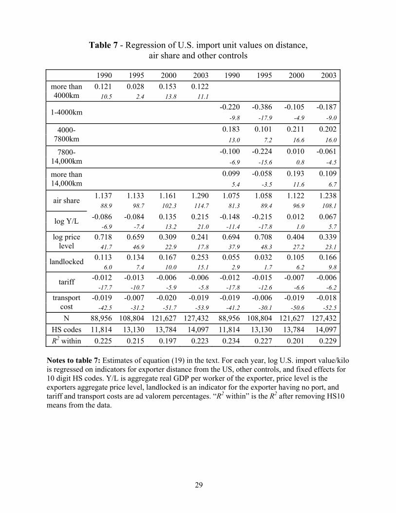
Tables 7 and 8 report the results of estimating equation (19), which is the same

specification as in equation (18) but with air share included as an explanatory variable. Airshare

is measured as a continuous variable, but almost all the observations on 10-digit codes are either

zero or one, so it is very close to a dummy variable for air shipment. The coefficient on air share

is large and statistically significant in every specification, ranging between 1.06 and 1.6. This

implies very large price effects, ranging between 290 and 500 percent. As expected, the distance

effect is much smaller when directly controlling for airshare, but is still generally positive and

statistically significant for distances greater than 4000km. This suggests that the sorting

mechanism of the model operates for surface-shipped as well as air-shipped goods, though the

air shipment sorting effect is more powerful.

4 Conclusion

This paper has focused on the interaction between trade, distance, product characteristics, and the

choice of shipping mode. In the theory model, I showed how the existence of airplanes implies

that distant countries have a comparative advantage in lightweight goods. In the empirical

section, I documented the heterogeneity across regions and goods of the prevalence of air

shipment in US imports. The statistical analysis uncovered a large and robust relationship

between distance and unit values: U.S. imports from remote suppliers have unit values on the

order of a third higher than those from nearby countries. Goods which are shipped by airfreight

have unit values that are much higher than those shipped by surface, even after controlling for

distance.

16

References

Deardorff, Alan, 2004, "Local Comparative Advantage: Trade Costs and the Pattern of Trade",

http://www.econ.lsa.umich.edu/~alandear/writings/

Eaton, Jonathan and Samuel Kortum, 2002, “Technology, Geography, and Trade”, Econometrica

70(5): 1741-1779 (September).

Evans, Carolyn E., and James Harrigan, 2005, “Distance, Time, and Specialization: Lean

Retailing in General Equilibrium”, forthcoming, American Economic Review.

Harrigan, James, and A.J. Venables, 2004, “Timeliness, Trade, and Agglomeration”, NBER

Working Paper 10404.

Hummels, David, 1999, “Have International Transportation Costs Declined?”,

http://www.mgmt.purdue.edu/faculty/hummelsd/

Hummels, David, 2001a, “Time as a Trade Barrier”,


Hummels, David, 2001b, “Toward a Geography of Trade Costs”,


Hummels, David, and Alexandre Skiba, 2004, “Shipping the Good Apples Out? An Empirical

Confirmation of the Alchian-Allen Conjecture”, Journal of Political Economy 112(6):

1384-1402 (December).

Hummels, David, and Peter Klenow, 2005, “The Variety and Quality of a Nation’s Exports”,

forthcoming, American Economic Review.

Leamer, Edward, 1984, Sources of International Comparative Advantage, Cambridge, MA: MIT

Press.

Limão, Nuno, and A.J. Venables, 2002, “Geographical Disadvantage: a Hecksher-Ohlin-Von-

Thunen Model of International Specialisation,” Journal of International Economics

58(2): 239-63 (December).

Redding, Stephen, and A.J. Venables, 2004, "Economic Geography and International

Inequality", Journal of International Economics 62(1): 53-82.

Schott, Peter K., 2004, “Across-product versus within-product specialization in international

trade”, Quarterly Journal of Economics119(2):647-678 (May).

17

Figure 1

Relative price of Air to Ocean shipping

90

100

110

120

130

140

150

160

170

1990 1991 1992 1993 1994 1995 1996 1997 1998 1999 2000 2001 2002 2003 2004

2000

= 1

00

Air / Ocean Air Asia / Ocean Pacific Notes to Figure 1: Data are price indices for U.S. imports of air freight and ocean liner shipping services from the Bureau of Labor Statistics, www.bls.gov/mxp. The “Air/Ocean” series divides all US imports of air freight services by all imports of ocean liner services, while the “Air Asia / Ocean Pacific” series divides the index for air freight imports from Asia by the index for ocean liner imports from the Pacific region.

18

Figure 2 - the air shipping decision

Figure 3 - Market shares for country 2

π

z0 1

1

2 ( )π L z

2 ( )π H z

π

z0 1

1

2 ( )π L z

2 ( )π H z

3τ

2τ

( )ω za

z0 1

3τ

2τ

( )ω za

z0 1

19

3τ

2τ

( )ω za

′zz0 1

( )ω′ za

3τ

2τ

( )ω za

′zz0 1

( )ω′ za

Figure 4 - Change in z when air freight costs fall

Figure 5 - Change in equilibrium market shares when air freight costs fall

π

z0 1

1

2 ( )π H z

′z

2 ( )π L zπ

z0 1

1

2 ( )π H z

′z

2 ( )π L z

20

Figure 6- Wages as a function of air freight costs

0.50.550.60.650.70.750.80.850.90.951

beta

0.0

0.5

1.0

1.5

2.0

2.5

w2 w3 w2/w3

Notes to Figure 6: Illustrates equilibrium wages as a function of air freight costs for a numerical example, with air freight costs varying from prohibitive (left axis) to low enough so that country 3 always uses air freight (right axis). Wage in country 3 is normalized to 1 when air transport cost is prohibitive. For parameter values used in numerical example, see appendix.

Chart 1

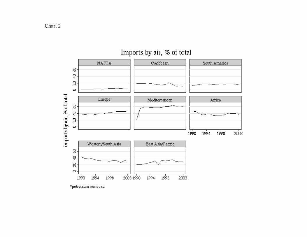
Chart 2

Chart 3

Chart 4

Chart 5

Chart 6

Chart 7

Chart 8

Chart 9

Chart 10

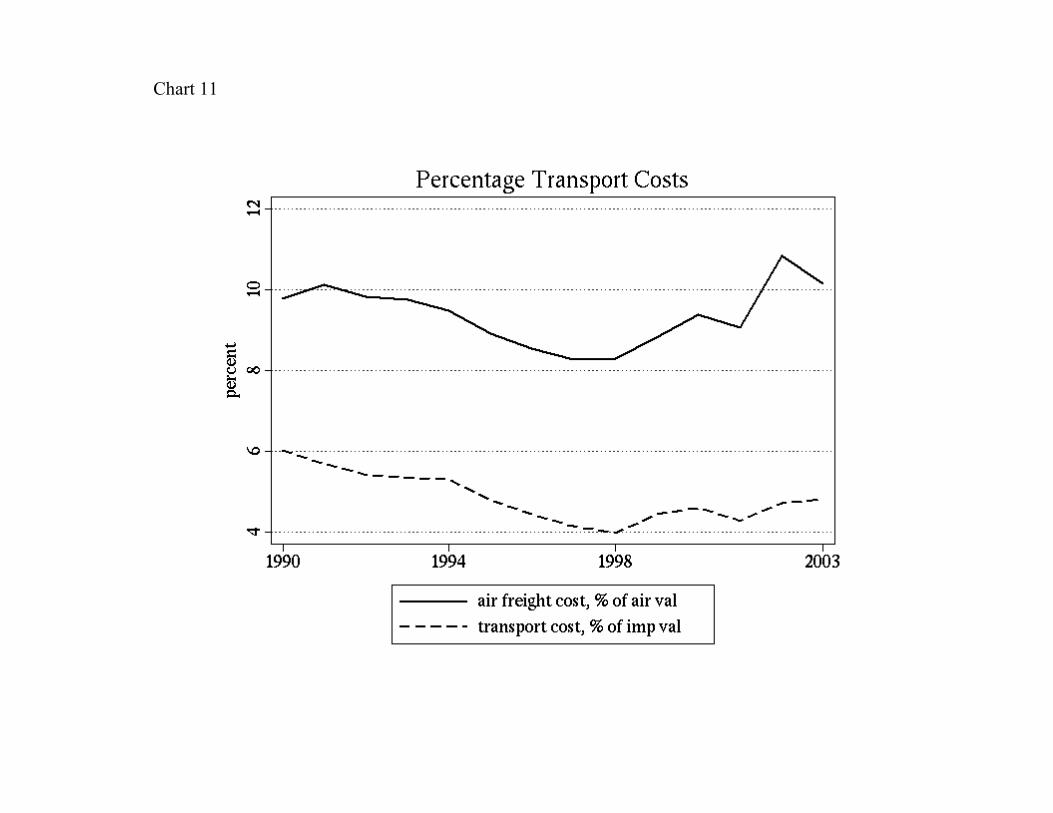
Chart 11

21

Table 1 Imports by product and percent air shipped, 1990 and 2003 Share of total

1990 2003 SITC2 Share of category

1990

Imports by air, % of

total 1990

Share of category

2003

Imports by air, % of

total 2003 SITC description

12.2 8.9 Petroleum 33 100.0 2.4 100.0 2.9 Petroleum, petroleum products and related materials

2.2 3.3 Other fuel & raw materials 28 35.0 9.1 7.5 13.6 Metalliferous ores and metal scrap 34 30.6 1.4 74.3 7.6 Gas, natural and manufactured 23 11.2 6.8 4.5 10.0 Crude rubber (including synthetic and reclaimed) 27 10.6 19.4 5.7 19.6 Crude fertilizers, other than those of division 56, and crude minerals 26 5.5 7.7 1.6 29.1 Textile fibres (other than wool tops and other combed wool) and their wastes 35 4.3 0.0 3.4 0.0 Electric current 32 2.7 1.7 2.9 0.3 Coal, coke and briquettes

3.4 2.8 Forest products 64 51.2 23.8 43.5 19.5 Paper, paperboard and articles of paper pulp, of paper or of paperboard 24 18.9 4.9 21.2 4.0 Cork and wood 25 17.3 12.3 7.6 9.5 Pulp and waste paper 63 12.6 18.3 27.7 13.0 Cork and wood manufactures (excluding furniture)

5.7 4.7 Animal and vegetable products 5 19.8 7.4 19.5 5.8 Vegetables and fruit 3 18.5 31.2 17.4 26.6 Fish (not marine mammals), crustaceans, molluscs and aquatic invertebrates 11 12.7 4.7 17.9 2.7 Beverages 7 12.0 6.2 9.0 8.2 Coffee, tea, cocoa, spices, and manufactures thereof 1 10.5 15.0 7.6 14.7 Meat and meat preparations 29 4.4 36.8 4.8 40.6 Crude animal and vegetable materials, n.e.s. 6 4.3 3.0 3.7 3.9 Sugars, sugar preparations and honey 0 4.3 86.6 2.8 83.8 Live animals other than animals of division 03 4 3.2 5.6 5.6 4.0 Cereals and cereal preparations 12 2.3 16.2 2.2 14.1 Tobacco and tobacco manufactures 42 2.3 3.7 2.3 6.6 Fixed vegetable fats and oils, crude, refined or fractionated 2 1.7 18.9 1.9 14.2 Dairy products and birds' eggs 9 1.4 6.9 3.2 7.9 Miscellaneous edible products and preparations 8 1.2 9.6 1.2 5.2 Feeding stuff for animals (not including unmilled cereals) 22 0.7 11.8 0.5 10.8 Oil-seeds and oleaginous fruits 21 0.6 44.2 0.2 61.1 Hides, skins and furskins, raw 43 0.2 3.1 0.3 10.3 Animal or vegetable fats and oils, processed; waxes of animal or vegetable origin 41 0.1 13.4 0.1 18.7 Animal oils and fats

22

Table 1, continued 15.3 15.9 Labor intensive manufactures

84 33.3 56.5 31.4 47.5 Articles of apparel and clothing accessories 89 32.9 47.0 32.6 46.4 Miscellaneous manufactured articles, n.e.s. 85 12.8 46.3 7.7 50.1 Footwear 66 11.6 28.9 13.7 24.5 Non-metallic mineral manufactures, n.e.s. 82 6.6 12.8 12.2 12.3 Furniture, and parts thereof; bedding, mattresses, mattress supports, cushions 83 2.9 60.9 2.3 58.2 Travel goods, handbags and similar containers

8.1 7.0 Capital intensive manufactures 67 24.5 3.3 14.5 7.1 Iron and steel 68 23.4 17.0 19.4 25.2 Non-ferrous metals 69 22.2 24.2 28.5 29.4 Manufactures of metals, n.e.s. 65 15.8 45.8 19.7 46.3 Textile yarn, fabrics, made-up articles, n.e.s., and related products 62 8.7 14.6 9.7 27.0 Rubber manufactures, n.e.s. 81 3.1 18.4 6.9 20.0 Prefabricated buildings; sanitary, plumbing, heating and lighting fixtures and 61 2.2 59.1 1.3 65.3 Leather, leather manufactures, n.e.s., and dressed furskins

45.2 45.0 Machinery 78 34.2 14.7 31.1 19.4 Road vehicles (including air-cushion vehicles) 77 15.0 55.3 14.6 60.9 Electrical machinery, apparatus and appliances, n.e.s., and electrical parts the 75 12.3 73.6 14.5 74.5 Office machines and automatic data-processing machines 76 9.7 57.6 12.7 74.5 Telecommunications and sound-recording and reproducing apparatus 74 6.4 31.5 6.8 34.7 General industrial machinery and equipment, n.e.s., and machine parts, n.e.s. 72 5.9 30.2 3.7 35.7 Machinery specialized for particular industries 71 5.8 40.1 5.7 43.9 Power-generating machinery and equipment 79 3.3 42.0 3.6 42.8 Other transport equipment 88 3.0 68.2 2.1 73.7 Photographic apparatus, equipment and supplies and optical goods, watches 87 2.7 64.0 4.2 75.5 Professional, scientific and controlling instruments and apparatus, n.e.s. 73 1.7 28.9 1.0 41.4 Metalworking machinery

4.5 8.3 Chemicals 51 32.7 23.4 33.5 32.2 Organic chemicals 52 14.0 11.1 7.1 16.8 Inorganic chemicals 54 11.7 54.6 31.2 65.0 Medicinal and pharmaceutical products 59 9.2 10.9 6.7 21.6 Chemical materials and products, n.e.s. 57 8.9 7.2 7.1 19.5 Plastics in primary forms 58 8.0 24.2 4.6 27.2 Plastics in non-primary forms 53 5.9 10.4 2.4 18.4 Dyeing, tanning and colouring materials 55 5.3 28.3 5.4 22.7 Essential oils and resinoids and perfume materials; toilet, polishing and cleanser 56 4.2 8.7 2.0 6.9 Fertilizers (other than those of group 272)

23

Table 2 Country categories

distance country region country region

Canada NAFTA Mexico NAFTA 1-4000 km from USA Bahamas Caribbean Barbados Caribbean

Belize Caribbean Costa.Rica Caribbean Dominican.Republic Caribbean El.Salvador Caribbean Guatemala Caribbean Haiti Caribbean Honduras Caribbean Jamaica Caribbean Nicaragua Caribbean Panama Caribbean Trinidad.And.Tobago Caribbean Colombia South America Venezuela South America Bolivia South America Brazil South America 4000-7800 km

from USA Ecuador South America Guyana South America Paraguay South America Peru South America Suriname South America Austria Europe Belgium-Lux Europe Czechoslovakia Europe Denmark Europe Finland Europe France Europe Germany Europe Hungary Europe Iceland Europe Ireland Europe Italy Europe Netherlands Europe Norway Europe Poland Europe Portugal Europe Spain Europe Sweden Europe Switzerland Europe United.Kingdom Europe Yugoslavia Europe Algeria Mediterranean Malta Mediterranean Morocco Mediterranean Tunisia Mediterranean Gambia Africa Guinea Africa Guinea.Bissau Africa Liberia Africa Mali Africa Mauritania Africa Senegal Africa Sierra.Leone Africa

25

Table 2, continued distance country region country region

Argentina South America Chile South America 7800-14000 km from USA Uruguay South America Bulgaria Europe

Romania Europe Russian.Federation Europe Cyprus Mediterranean Egypt Mediterranean Greece Mediterranean Israel Mediterranean Syrian.Arab.Republic Mediterranean Turkey Mediterranean Angola Africa Benin Africa Burkina.Faso Africa Burundi Africa Cameroon Africa Central.African.Republic Africa Chad Africa Comoros Africa Congo Africa Cote.D'Ivour Africa Djibouti Africa Ethiopia Africa Gabon Africa Ghana Africa Kenya Africa Malawi Africa Mozambique Africa Niger Africa Nigeria Africa Rwanda Africa Somalia Africa South.Africa Africa Sudan Africa Tanzania Africa Togo Africa Uganda Africa Zaire Africa Zambia Africa Zimbabwe Africa Afghanistan Western/South Asia Bahrain Western/South Asia Bangladesh Western/South Asia Bhutan Western/South Asia India Western/South Asia Iran Western/South Asia Iraq Western/South Asia Jordan Western/South Asia Kuwait Western/South Asia Mongolia Western/South Asia Myanmar Western/South Asia Nepal Western/South Asia Oman Western/South Asia Pakistan Western/South Asia Qatar Western/South Asia Saudi.Arabia Western/South Asia United.Arab.Emirates Western/South Asia Yemen Western/South Asia China East Asia/Pacific Fiji East Asia/Pacific Hong.Kong East Asia/Pacific Japan East Asia/Pacific Korea.RP.(S) East Asia/Pacific Laos East Asia/Pacific Phillipines East Asia/Pacific Solomon.Islands East Asia/Pacific Taiwan East Asia/Pacific Madagascar Africa Mauritius Africa over 14000 km

from USA Seychelles Africa Reunion.Islands Western/South Asia Sri.Lanka Western/South Asia Australia East Asia/Pacific Indonesia East Asia/Pacific Malaysia East Asia/Pacific New.Zealand East Asia/Pacific Papua.New.Guinea East Asia/Pacific Singapore East Asia/Pacific Thailand East Asia/Pacific

26

Table 3- Transport costs by region

transport cost, % of import

value

air freight cost, % of air value

Region 2003 2003

NAFTA 1.50 5.17 Caribbean 2.34 6.47 South America 9.17 7.04 Europe 4.45 4.96 Mediterranean 5.09 10.18 Africa 7.02 14.57 Western/South Asia 7.12 15.38 East Asia/Pacific 6.17 12.76 Table 4- Transport costs by product

transport cost, % of import

value

air freight cost, % of air value

Product 2003 2003

Petroleum 5.00 22.37

Other fuel & raw materials 4.74 3.76

Forest products 6.44 20.88

Animal and vegetable products 7.30 23.77

Labor intensive manufactures 5.71 4.43

Capital intensive manufactures 5.48 6.97

Machinery 1.97 2.37

Chemicals 2.73 1.04

27

Table 5 - Regression of U.S. import unit values on distance and other controls

1990 1995 2000 2003 1990 1995 2000 20030.260 0.190 0.371 0.362 more than

4000km 21.6 15.3 32.8 31.9

0.056 -0.148 0.092 0.0471-4000km

2.4 -6.6 4.2 2.2

0.446 0.390 0.517 0.5304000-7800km 31.4 27.4 40.4 41.3

-0.023 -0.133 0.139 0.0787800-14,000km -1.5 -8.9 9.8 5.5

0.239 0.074 0.355 0.290more than 14,000km 12.6 4.3 20.6 17.0

-0.051 -0.056 0.200 0.276 -0.130 -0.202 0.031 0.081log Y/L -4.0 -4.7 18.7 25.7 -9.6 -16.1 2.5 6.6

0.829 0.769 0.403 0.364 0.760 0.768 0.485 0.445log price level 46.0 52.3 28.7 25.7 39.9 50.3 31.6 29.0

0.294 0.322 0.337 0.443 0.178 0.154 0.217 0.291landlocked 14.8 16.96 19.41 25 9.0 8.2 12.4 16.3

-0.014 -0.011 -0.001 -0.003 -0.013 -0.013 -0.002 -0.002tariff -18.5 -8.7 -0.8 -3.0 -18.1 -9.9 -1.5 -1.9

-0.012 -0.004 -0.013 -0.011 -0.012 -0.004 -0.013 -0.011transport cost -25.4 -18.2 -33.5 -30.1 -25.9 -18.3 -32.7 -29.4

N 88,984 108,837 121,830 127,602 88,984 108,837 121,830 127,602HS codes 11,815 13,131 13,788 14,103 11,815 13,131 13,788 14,103R2 within 0.145 0.135 0.119 0.132 0.168 0.162 0.131 0.149

Notes to Table 5: Estimates of equation (18) in the text. For each year, log U.S. import unit value is regressed on indicators for exporter distance from the US, other controls, and fixed effects for 10 digit HS codes. Y/L is aggregate real GDP per worker of the exporter, price level is the exporters aggregate price level, landlocked is an indicator for the exporter having no port, and tariff and transport costs are ad valorem percentages. “R2 within” is the R2 after removing HS10 means from the data.

28

Table 6 - Regression of U.S. import value/kilo on distance and other controls

1990 1995 2000 2003 1990 1995 2000 20030.400 0.353 0.551 0.510 more than

4000km 36.1 30.2 50.2 45.8

0.296 0.069 0.160 0.1651-4000km

14.5 3.4 8.0 8.3

0.571 0.508 0.657 0.6564000-7800km 41.6 36.5 51.4 50.8

0.339 0.229 0.461 0.3457800-14,000km 23.3 15.7 32.8 24.1

0.443 0.334 0.598 0.494more than 14,000km 24.3 19.8 35.1 28.9

-0.057 -0.096 0.058 0.151 -0.056 -0.153 -0.016 0.042log Y/L -4.9 -8.6 5.8 14.7 -4.5 -12.6 -1.4 3.6

0.718 0.746 0.523 0.488 0.643 0.721 0.550 0.511log price level 43.4 53.3 39.2 35.7 36.7 49.1 37.8 34.9

0.362 0.327 0.374 0.478 0.310 0.249 0.320 0.384landlocked 18.9 18.0 22.2 27.2 16.2 13.7 18.7 21.6

-0.013 -0.009 -0.002 -0.001 -0.014 -0.010 -0.003 -0.001tariff -10.8 -7.7 -2.4 -1.5 -11.5 -8.8 -3.7 -1.1

-0.014 -0.004 -0.015 -0.014 -0.015 -0.004 -0.016 -0.014transport cost -33.9 -21.8 -41.9 -39.2 -35.2 -22.2 -42.1 -39.3


Notes to Table 6: Estimates of equation (18) in the text. For each year, log U.S. import value/kilo is regressed on indicators for exporter distance from the US, other controls, and fixed effects for 10 digit HS codes. Y/L is aggregate real GDP per worker of the exporter, price level is the exporters aggregate price level, landlocked is an indicator for the exporter having no port, and tariff and transport costs are ad valorem percentages. “R2 within” is the R2 after removing HS10 means from the data.

29

Table 7 - Regression of U.S. import unit values on distance, air share and other controls

1990 1995 2000 2003 1990 1995 2000 2003

0.121 0.028 0.153 0.122 more than 4000km 10.5 2.4 13.8 11.1

-0.220 -0.386 -0.105 -0.1871-4000km

-9.8 -17.9 -4.9 -9.0

0.183 0.101 0.211 0.2024000-7800km 13.0 7.2 16.6 16.0

-0.100 -0.224 0.010 -0.0617800-14,000km -6.9 -15.6 0.8 -4.5

0.099 -0.058 0.193 0.109more than 14,000km 5.4 -3.5 11.6 6.7

1.137 1.133 1.161 1.290 1.075 1.058 1.122 1.238air share 88.9 98.7 102.3 114.7 81.3 89.4 96.9 108.1

-0.086 -0.084 0.135 0.215 -0.148 -0.215 0.012 0.067log Y/L -6.9 -7.4 13.2 21.0 -11.4 -17.8 1.0 5.7

0.718 0.659 0.309 0.241 0.694 0.708 0.404 0.339log price level 41.7 46.9 22.9 17.8 37.9 48.3 27.2 23.1

0.113 0.134 0.167 0.253 0.055 0.032 0.105 0.166landlocked 6.0 7.4 10.0 15.1 2.9 1.7 6.2 9.8

-0.012 -0.013 -0.006 -0.006 -0.012 -0.015 -0.007 -0.006tariff -17.7 -10.7 -5.9 -5.8 -17.8 -12.6 -6.6 -6.2

-0.019 -0.007 -0.020 -0.019 -0.019 -0.006 -0.019 -0.018transport cost -42.5 -31.2 -51.7 -53.9 -41.2 -30.1 -50.6 -52.5


Notes to table 7: Estimates of equation (19) in the text. For each year, log U.S. import value/kilo is regressed on indicators for exporter distance from the US, other controls, and fixed effects for 10 digit HS codes. Y/L is aggregate real GDP per worker of the exporter, price level is the exporters aggregate price level, landlocked is an indicator for the exporter having no port, and tariff and transport costs are ad valorem percentages. “R2 within” is the R2 after removing HS10 means from the data.

30

Table 8 - Regression of U.S. import value/kilo on distance, air share, and other controls

1990 1995 2000 2003 1990 1995 2000 2003

0.266 0.187 0.292 0.221 more than 4000km 27.0 17.9 30.2 23.0

0.000 -0.184 -0.033 -0.0891-4000km

0.0 -10.3 -1.9 -5.2

0.251 0.159 0.257 0.2344000-7800km 20.1 12.5 22.5 20.6

0.254 0.125 0.319 0.1987800-14,000km 19.7 9.6 26.1 16.2

0.340 0.209 0.445 0.332more than 14,000km 21.0 13.8 30.1 22.7

1.274 1.260 1.443 1.599 1.292 1.271 1.476 1.606air share 114.4 124.1 147.5 164.6 111.3 120.7 147.5 161.9

-0.084 -0.112 -0.025 0.081 -0.072 -0.157 -0.043 0.028log Y/L -8.1 -11.2 -2.8 9.2 -6.6 -14.6 -4.2 2.8

0.574 0.604 0.390 0.303 0.557 0.641 0.441 0.363log price level 39.3 48.3 33.5 26.0 35.9 48.8 34.9 28.9

0.144 0.108 0.150 0.216 0.147 0.087 0.161 0.198landlocked 8.5 6.6 10.2 14.4 8.7 5.3 10.9 13.0

-0.010 -0.012 -0.011 -0.006 -0.009 -0.014 -0.012 -0.008tariff -8.9 -12.4 -13.6 -7.8 -8.9 -14.5 -14.9 -10.1

-0.023 -0.006 -0.025 -0.025 -0.024 -0.006 -0.026 -0.026transport cost -61.3 -39.9 -77.4 -83.5 -61.5 -40.1 -79.0 -84.2


Notes to table 8: Estimates of equation (19) in the text. For each year, log U.S. import value/kilo is regressed on indicators for exporter distance from the US, other controls, and fixed effects for 10 digit HS codes. Y/L is aggregate real GDP per worker of the exporter, price level is the exporters aggregate price level, landlocked is an indicator for the exporter having no port, and tariff and transport costs are ad valorem percentages. “R2 within” is the R2 after removing HS10 means from the data.

airplanes and comparative advantage

Documents